Stochastic stability of invariant measures: The 2D Euler equation

Abstract

In finite-dimensional dissipative dynamical systems, stochastic stability provides the selection of the physical relevant measures. That this might also apply to systems defined by partial differential equations, both dissipative and conservative, is the inspiration for this work. As an example the 2D Euler equation is studied. Among other results this study suggests that the coherent structures observed in 2D hydrodynamics are associated to configurations that maximize stochastically stable measures uniquely determined by the boundary conditions in dynamical space.

1 Introduction

The main purpose of this research is to extend the notion of stochastically stable invariant measure to dynamical systems defined by partial differential equations, in particular to conservative systems with many invariant measures where the notion of stochastic stability may provide a selection criteria for the physically relevant measures. In the following subsections and also partly in Section 2 and 3 some standard material is formulated in a notation appropriate for the further developments. The main original results are contained in the Section 4 and 5. The most direct physical implication would be the interpretation of the coherent structures observed in two-dimensional and quasi-two-dimensional fluid motion as configurations maximizing stochastically stable invariant measures. According to the results, the stochastically stable invariant measures would be unique for each choice of boundary conditions in the dynamical variables.

1.1 The physical relevance of stochastically stable invariant measures

For finite-dimensional systems the notions of physical measure and stochastically stable measure are closely related. Let $M$ be the state space, $f:M\rightarrow M$ a dynamical system defined by a smooth transformation and $\mu$ a positive Borel measure on $M$ such that

$$\lim_{n\rightarrow\infty}\frac{1}{n}\sum_{j=0}^{n-1}\varphi\left(f^{j}\left(x\right)\right)\rightarrow\int_{M}\varphi d\mu$$ (1)

for a positive measure set $A$ of initial points $x$ and any continuous function $\varphi:M\rightarrow\mathbb{R}$. It means that time averages of continuous functions are given by the corresponding spatial averages computed with respect to $\mu$, at least for a large set of initial states $x$. Such measure $\mu$, when it exists, is called a physical measure (or Sinai-Bowen-Ruelle, SBR measure) [1] [2] [3] [4].

For uniformly hyperbolic systems there is a complete theory concerning existence and uniqueness of physical measures and partial results for non-uniformly hyperbolic and partially hyperbolic systems [5] [6].

Consider now the stochastic process $f_{\varepsilon}$ obtained by adding a small random noise to the deterministic system $f$. Under very general conditions, there exists a stationary probability measure $\mu_{\varepsilon}$ such that, almost surely,

$$\lim_{n\rightarrow\infty}\frac{1}{n}\sum_{j=0}^{n-1}\varphi\left(f_{\varepsilon}^{j}\left(x\right)\right)\rightarrow\int\varphi d\mu_{\varepsilon}$$ (2)

Stochastic stability of the $\mu$ measure means that $\mu_{\varepsilon}$ converges to the physical measure $\mu$ when the noise level $\varepsilon$ goes to zero. There is stochastic stability for uniformly hyperbolic maps, for Lorenz strange attractors, Hénon strange attractors and also general results for partially hyperbolic systems [7] [8] [9] [10] [11] [12]. Existence and uniqueness of the invariant measure $\mu_{\varepsilon}$ under general conditions provides a powerful tool to obtain the relevant physical measure of the dynamical system $f$, by randomly perturbing it and then letting the noise level $\varepsilon\rightarrow 0$.

In the past, stochastic stability of the physical measures has been considered mostly relevant for dissipative systems or for Hamiltonian systems with small dissipative perturbations. That the same notion might also be useful for strictly conservative systems follows from our results, with the choice of boundary conditions in the dynamical space leading to uniqueness of the stochastically stable measure.

1.2 The 2D Euler equation and persistent large-scale structures in (quasi) two dimensional fluid motion

For definiteness, our study concentrates on the stability of invariant measures for the 2D Euler equation, an issue of current physical interest for the understanding of geophysical phenomena [13] [14]. A striking feature of (quasi) two-dimensional turbulent fluid motion [13] is the emergence of large scale structures which persist for long time intervals. Another feature is the relaxation of the flow to a small number of patterns, as if they were attractors of the dynamics, a feature not to be expected in conservative or small dissipation systems. This last feature, is also contrary to the idea that viscosity is required to explain irreversibility in turbulent flows. These phenomena should hopefully be explained by the 2D Euler equation or by its quasi-geostrophic variants.

It has been suggested by many authors that the behavior of turbulent two-dimensional flows should be understood by the methods of equilibrium or non-equilibrium statistical mechanics ([15] [16] [17] [18] [19] [13] and references therein). Modern studies in this direction concentrate in construction of microcanonical or more general invariant Young measures, on their relation to the small viscosity limit of the invariant measures of Navier-Stokes, relaxation of the dynamics and phase transitions.

Here, following the inspiration provided by the results on physical measures, as described above, we study the stochastic stability of the invariant measures. The plan of the paper is as follows: in Section 2, infinitesimally invariant measures of partial differential equations are related to the generator of the flow and in Section 3 the 2D Euler equation with periodic boundary conditions is written as a differential equation for its Fourier modes and it is shown that it has infinitely many invariant measures.

In Section 4.1 we revisit the question already addressed by other authors [20] [21] of whether an invariant measure of the 2D Euler equation remains invariant when the deterministic flow is replaced by an Ornstein-Uhlenbeck process. Some such measures are found, which however correspond both to a noise perturbation and to a change of the deterministic vector field. Therefore they are not candidates for the stochastically stable measures in the sense described before. Then in Section 4.2, we add a noise perturbation to the deterministic dynamics and show that once a boundary condition on the dynamical space is fixed, there is a unique measure which converges in the sense of viscosity solutions to a measure density of the deterministic equation. This result is obtained for the 2D Euler equation truncated to arbitrarily large $N$ Fourier modes. How to generalize it to the infinite-dimensional case is indicated.

The result obtained in 4.2 provides a reasonable interpretation of the stability of the large scale structures in two-dimensional fluid motion. Because the stochastically stable invariant measure depends on the boundary conditions (for example a cut-off at large modes), we also understand why, depending on the particular physical environment, the structures display not a unique but several different shapes. It also provides a plausible explanation for the relaxation of the flow to selected structures, not as an effect of some residual viscosity but as a result of the noise always present in a physical system. In addition the dependence of the stochastically stable measure on the dynamical boundary conditions might also provide an explanation of why the same basic equation may lead to different large scale patterns depending on the physical environment.

Finally, in Section 5, we briefly rephrase our results in configuration space and using a recently developed stable algorithm perform a few illustrative numerical simulations of a finite mode 2D Euler equation perturbed by noise that show the emergence of the stochastically stable patterns.

Most of the results in the paper refer to a truncated system, therefore to an arbitrarily large, but finite, dynamical system. The actual extension to an infinite system is sketched but not worked out in detail.

2 Infinitesimally invariant measures of partial differential equations

Let $\Gamma_{t}$ be the flow of a partial differential equation and $\Gamma_{t}^{\ast}$ the push-forward semigroup acting on measures. A measure $\mu$ is invariant if

$$\Gamma_{t}^{\ast}\left(\mu\right)=\mu$$ (3)

and infinitesimally invariant if

$$\int B\varphi d\mu=0$$ (4)

for any differentiable function $\varphi$, $B$ being the generator of the flow $\Gamma_{t}$. Equivalently $B^{\ast}1=0$.

Let the generator $B$ be a first or second order differential operator on a discrete set of coordinates $\phi=\left\{\phi_{i}\right\}$,

$$B=\sum_{i,j}u_{ij}\left(\phi\right)\frac{\partial^{2}}{\partial\phi_{i}\partial\phi_{j}}+\sum_{i}b_{i}\left(\phi\right)\frac{\partial}{\partial\phi_{i}}$$ (5)

and consider a measure of the form

$$d\mu=R\left(\phi\right)\prod_{i}d\phi_{i}$$ (6)

To obtain the condition (4)

$$\int\left(B\varphi\right)R\left(\phi\right)\prod_{i}d\phi_{i}=0$$

one computes the adjoint of $B$ obtaining

$$B^{\ast} = -\frac{1}{R}\left\{\sum_{i}\frac{\partial}{\partial\phi_{i}}\left(Rb_{i}\right)-\sum_{i,j}\frac{\partial^{2}}{\partial\phi_{i}\partial\phi_{j}}\left(Ru_{ij}\right)\right\}$$ (7)

$$+\sum_{i}\left\{-b_{i}+\frac{1}{R}\sum_{j}\frac{\partial}{\partial\phi_{j}}\left[R\left(u_{ij}+u_{ji}\right)\right]\right\}\frac{\partial}{\partial\phi_{i}}+\sum_{i,j}u_{ij}\frac{\partial^{2}}{\partial\phi_{i}\partial\phi_{j}}$$

Therefore, to have $B^{\ast}1=0$, the first term in (7) should vanish leading to

Proposition 1: A generator $B$ of the form in Eq.(5), $u_{ij}$ and $b_{i}$ being differentiable functions, has

$$d\mu=R\left(\phi\right)\prod_{i}d\phi_{i}$$

($R\left(\phi\right)$ differentiable) as an infinitesimally invariant measure if and only if

$$\sum_{i}\frac{\partial}{\partial\phi_{i}}\left(Rb_{i}\right)-\sum_{i,j}\frac{\partial^{2}}{\partial\phi_{i}\partial\phi_{j}}\left(Ru_{ij}\right)=0$$ (8)

Equivalently

$$b_{i}=\frac{1}{R}\sum_{j}\frac{\partial}{\partial\omega_{j}}\left(Ru_{ij}\right)+\frac{X_{i}}{R}$$ (9)

where $X_{i}$ is an arbitrary function satisfying $\sum_{i}\frac{\partial X_{i}}{\partial\phi_{i}}=0$.

A similar result has been obtained in [22].

3 The 2D Euler equation on the torus

Consider the 2D Euler equations for an inviscid incompressible fluid

$$\left\{\begin{array}[]{l}{\frac{\partial v}{\partial t}}=-(v\cdot\nabla)v-\nabla p\\ div\ v=0\end{array}\right.$$ (10)

subjected to periodic boundary conditions and initial data

$$v(x,0)=v_{0}(x),$$ (11)

where $v(x,t)=(v_{1}(x_{1},x_{2},t),v_{2}(x_{1},x_{2},t))$ is the velocity field of the fluid and $p=p(x,t)$ is the pressure.

Since $div\ v=0$ and $div\ v_{0}=0,$ there is a function $\psi(x,t)$ (the stream function) such that

$$v=\nabla^{\perp}\psi=(-\partial_{x_{2}}\psi,\partial_{x_{1}}\psi)$$ (12)

and the Euler equation becomes

$$\partial_{t}\Delta\psi=-\nabla^{\perp}\psi\cdot\nabla\Delta\psi$$ (13)

As in [20] we consider solutions of (13) on the 2-dimensional flat torus, a square in $\mathbb{R}^{2}$ with periodic boundary conditions, $T^{2}=[0,1]\times[0,1]$,

$$\psi(0,x_{2},t)=\psi(1,x_{2},t),\;\;\;\;\;\;\;\;\;\psi(x_{1},0,t)=\psi(x_{1},1,t)$$ (14)

$\forall x=(x_{1},x_{2})\in T^{2},\forall t\in[0,T].$ Let us denote by $e_{k}(x)=e^{i\,2\pi k\cdot x},$  $k\in\mathbb{Z}^{2}$ the eigenfunctions for the operator $-\Delta$ with eigenvalues $4\pi^{2}\left(k_{1}^{2}+k_{2}^{2}\right)$, where $k\cdot x=k_{1}x_{1}+k_{2}x_{2}$. They form a complete set of orthonormal functions in $L^{2}(T^{2})$. We expand the solution $\psi(x,t)$ of (13) as a Fourier series

$$\psi(x,t)=\sum_{k}\phi_{k}(t)e_{k}(x).$$

Since $\psi$ is a real function and we can assume $\int_{T^{2}}\psi dx=0$, then $\phi_{-k}=\overline{\phi}_{k}$ ($\overline{z}$ being the complex conjugate of $z$) and

$$\psi(x,t)=\sum_{k\in\mathbb{Z}_{+}^{2}}\phi_{k}(t)e_{k}(x),$$ (15)

where $\mathbb{Z}_{+}^{2}$ denotes the set $\{k\in\mathbb{Z}^{2}:\ k_{1}>0,\ k_{2}\in\mathbb{Z}\text{ or }k_{1}=0,\ k_{2}>0\}$.

By (15), the function $\psi$ is identified with an infinite vector of Fourier coefficients

$$\psi=\left\{\phi_{k}\right\}_{k\in\mathbb{Z}_{+}^{2}}$$

where$\ k\in\mathbb{Z}_{+}^{2}$. We define $\mathbb{C}^{\infty}=\left\{\phi=\left\{\phi_{k}\right\}_{k\in\mathbb{Z}_{+}^{2}}\ :\ \phi_{k}\in\mathbb{C}\right\}.$

Substituting (15) in equation (13) and introducing the operator [20] [23] [21]

$$B(\phi)=\left\{B_{k}(\phi)\right\}_{k\in\mathbb{Z}_{+}^{2}}=\sum_{k}B_{k}(\phi)\frac{\partial}{\partial\phi_{k}}$$

with coefficients $B_{k}=B_{k}(\omega)$

$$B_{k}(\phi)=\frac{4\pi^{2}}{k^{2}}\sum_{\begin{subarray}{c}h\neq k\\ h,k\in\mathbb{Z}_{+}^{2}\end{subarray}}\left(k^{\bot}\cdot h\right)\left(k-h\right)^{2}\phi_{h}\phi_{k-h}$$ (16)

where $k^{\bot}=(-k_{2},k_{1})$, the system (10) becomes the following infinite dimensional ordinary differential equation

$$\frac{d}{dt}\phi_{k}=B_{k}(\phi)\hskip 14.22636ptk\in\mathbb{Z}_{+}^{2}$$ (17)

and

$$\frac{\partial B_{k}}{\partial\phi_{k}}=0$$ (18)

We may now find the (infinitesimally) invariant measures of the Euler equation on the torus. For the measure (6) we see from (5) that with $u_{ij}\left(\phi\right)=0$, the condition (8) is simply

$$\sum_{i}\frac{\partial}{\partial\phi_{i}}\left(Rb_{i}\right)=0$$

that is,

$$\sum_{i}\frac{\partial}{\partial\phi_{i}}\left(RB_{i}\right)=0$$

or from (18)

$$\sum_{i}B_{i}\frac{\partial}{\partial\phi_{i}}R=\sum_{i}\frac{d}{dt}\phi_{i}\frac{\partial}{\partial\phi_{i}}R=\frac{d}{dt}R=0$$

In conclusion: any constant of motion of the Euler equation generates an (infinitesimally) invariant measure. Among them we mention the energy $E$ and the enstrophy $S$ (or functions thereof) which in this setting read

$$E=\frac{1}{2}\sum_{k}k^{2}\phi_{k}^{2}$$

$$S=\frac{1}{2}\sum_{k}k^{4}\phi_{k}^{2}$$

The Poisson structure of the Euler 2D equation being degenerate, there is a set of Casimir invariants [24], which are invariant for any Hamiltonian flow with that Poisson structure. In this case they are

$$C_{f}=\int f\left(\triangle\psi\right)d^{2}x$$

$f$ being an arbitrary differentiable function. Therefore there are infinitely many invariant measures for the 2D Euler equation. The enstrophy is the Casimir invariant for $f\left(x\right)=x^{2}$.

4 Stochastic perturbations of the 2D Euler equation and invariant measures

Here we discuss stochastic stability of invariant measures in two different settings. First, given an invariant measure of the deterministic equation, we find the stochastic perturbation which preserves that measure when also the deterministic part is allowed to change. Second, we discuss the invariant measures of the stochastically perturbed system, with the deterministic part kept fixed and also the convergence of the perturbed measure when the perturbation tends to zero. It is this second study that is in the spirit of the identification of the physical measure by stochastic perturbations as it is done for finite-dimensional dissipative systems.

4.1 Stochastic perturbations preserving a deterministic invariant measure

A similar such study has been performed before and we use the same setting and notation as in [20] [21]. We introduce the Sobolev spaces of order $\beta\in\mathbb{R}$ on the torus $T^{2}$

$$H^{\beta} = \left\{\phi=\sum_{k}\phi_{k}e_{k}:\sum_{k}\left|k\right|^{2\beta}\left|\phi_{k}\right|^{2}<+\infty,\phi_{-k}=\overset{-}{\phi_{k}}\right\}$$ (19)

$$\equiv \left\{\phi=\left(\phi_{k}\right)_{k\in\mathbb{Z}_{+}^{2}}\in\mathbb{C}^{\infty}:\sum_{k\in\mathbb{Z}_{+}^{2}}\left|k\right|^{2\beta}\left|\phi_{k}\right|^{2}<+\infty\right\}$$

The spaces $H^{\beta}$ are complex Hilbert spaces with inner product and norm given by

$$<\phi^{(1)},\phi^{(2)}>_{H^{\beta}}=\sum_{k\in\mathbb{Z}_{+}^{2}}\left|k\right|^{2\beta}\phi_{k}^{(1)}\overline{\phi}_{k}^{(2)},\qquad\|\phi\|_{H^{\beta}}^{2}=<\phi,\phi>_{H^{\beta}}.$$

Definition: An arbitrary complex function $f=f(\phi):C^{\infty}\rightarrow C$ is a cylindrical function if, for some integer $N$, we have $f=f(\phi)\equiv F(\phi_{\alpha_{1}},\dots,\phi_{\alpha_{d(N)}})$, where $F$ is a $C_{0}^{1}(C^{N})$ - smooth function depending only on the components $\phi_{\alpha_{i}}$, $\alpha_{i}\in Z_{+,d(N)}^{2}$.

Let us consider the following infinite dimensional parametric Ornstein-Uhlenbeck operator $\varepsilon Q$ defined by

$$\varepsilon Qf(\phi)=\varepsilon\sum_{k}\left\{a_{k}\left(\phi\right)\frac{\partial}{\partial\phi_{k}}f(\phi)+\sigma_{k}\left(\phi\right)\frac{\partial^{2}}{\partial\phi_{k}^{2}}f(\phi)\right\}$$ (20)

for every cylindrical function.

If we consider the operator

$$Lf(\phi)=\varepsilon Qf(\phi)+\sum_{k}B_{k}(\phi)\frac{\partial}{\partial\phi_{k}}f(\phi)$$ (21)

we can see this operator as the infinitesimal generator for a stochastically perturbed Euler flow.

Let $W(t)=\sum_{k}\frac{1}{|k|}b_{k}(t)e_{k}$ be a normalized cylindrical brownian motion on $H^{1-\delta}$, $b_{k}(t)$ being independent copies of a complex brownian motion. To the generator (21) corresponds the following perturbed Euler equation

$$X_{k}(t)=X_{k}\left(0\right)+\int_{0}^{t}\left\{B_{k}\left(X\left(s\right)\right)+\varepsilon a\left(X_{k}(s)\right)\right\}ds+\int_{0}^{t}\sqrt{2\varepsilon\sigma_{k}\left(X_{k}(s)\right)}db_{k}(s),\,\,\,\,\forall k\in\mathbb{Z}_{+}^{2}.$$ (22)

Proposition 2: If $d\mu=R\left(\phi\right)\prod_{i}d\phi_{i}$ is an invariant measure for the (truncated) unperturbed Euler equation, then this is also an invariant measure for the perturbed equation (22) if $a_{k}\left(\phi\right)$ and $\sigma_{k}\left(\phi\right)$ in (20) satisfy

$$\sum_{k}\left\{\left(a_{k}-2\frac{\partial\sigma_{k}}{\partial\phi_{k}}\right)\frac{\partial R}{\partial\phi_{k}}+R\left(\frac{\partial a_{k}}{\partial\phi_{k}}-\frac{\partial^{2}\sigma_{k}}{\partial\phi_{k}^{2}}\right)-\sigma_{k}\frac{\partial^{2}R}{\partial\phi_{k}^{2}}\right\}=0$$ (23)

This is a direct consequence of Eq.(8). As an example, for the Gaussian measure constructed from the enstrophy

$$d\mu_{S}=e^{-\frac{1}{2}\sum_{k}k^{4}\phi_{k}^{2}}\prod_{j}d\phi_{j}$$ (24)

Eq.(23) is satisfied by

$$a_{k}=-k^{2}\phi_{k},\hskip 14.22636pt\sigma_{k}=\frac{1}{k^{2}}$$ (25)

and for the Gaussian measure constructed from the renormalized energy

$$d\mu_{E}=e^{-:E:}\prod_{j}d\phi_{j}$$ (26)

$$a_{k}=-\phi_{k},\hskip 14.22636pt\sigma_{k}=\frac{1}{k^{2}}$$ (27)

where $:E:=\frac{1}{2}\left(\sum_{k}k^{2}\phi_{k}^{2}-\mathbb{E}\left[\sum_{k}k^{2}\phi_{k}^{2}\right]\right)$.

Notice that in (24) and (26) we are considering a truncation of the 2D Euler equation to arbitrarily large $N$ modes. In the $N\rightarrow\infty$ limit the flat measure $\prod_{j}d\phi_{j}$ makes no sense and another reference measure should be used.

One sees that for these invariant measures of the unperturbed Euler equation, there are specific Ornstein-Uhlenbeck perturbations that preserve it as an invariant measure. However, in each case we are not only adding noise but also modifying the deterministic part. In the first (enstrophy) case we are actually adding noise to a Navier-Stokes equation

$$\begin{array}[]{ccc}\partial_{t}\Delta\psi&=&-\nabla^{\perp}\psi\cdot\nabla\Delta\psi+\varepsilon\triangle^{2}\psi\\ {\frac{\partial v}{\partial t}}&=&-(v\cdot\nabla)v+\varepsilon\triangle v-\nabla p\end{array}$$

and in the renormalized energy case

$$\begin{array}[]{ccc}\partial_{t}\Delta\psi&=&-\nabla^{\perp}\psi\cdot\nabla\Delta\psi-\varepsilon\triangle\psi\\ {\frac{\partial v}{\partial t}}&=&-(v\cdot\nabla)v-\varepsilon v-\nabla p\end{array}$$

Therefore, because invariance of these measures requires a fine tuning with both the deterministic and the stochastic components being modified with the same intensity $\varepsilon$, they do not seem to be the right candidates for the physical measures of the 2D Euler equation. The same applies to the results of Kuksin [26] who, using a viscosity of intensity $\varepsilon$ and a $\sqrt{\varepsilon}$ noise, shows that the collection of unique invariant measures so obtained is tight and converges in the $\varepsilon\rightarrow 0$ limit to a measure of the deterministic Euler equation.

Incidentally, also the microcanonical measures, that have been studied by a number of authors, do not seem to qualify as stochastically stable measures even with reasonable modifications of the deterministic part of the equation.

That the selection of a unique invariant measure requires a fine tuning, of both the noise and the deterministic terms, makes these, otherwise interesting, results irrelevant for the interpretation of physical phenomena, where such fine tuning is not to be expected.

4.2 The zero noise limit of the invariant measure of a stochastic system

In the previous subsection we have dealt with stochastic perturbations which preserve invariant measures of (17). As stated before, of more interest for the characterization of the physical measures would be to find noise-perturbed systems with an unique invariant measure and to construct the zero-noise limit of that measure. This we discuss now, not for the infinite dimensional system but again for its Galerkin approximations of arbitrary order $N$ [27]

$$\frac{d}{dt}\phi_{k}=B_{k}^{N}(\phi)\hskip 14.22636ptk\in\mathbb{Z}_{0}^{2}\hskip 22.76228pt\left|k\right|\leq N$$ (28)

$$B_{k}^{N}(\phi)=\frac{4\pi^{2}}{k^{2}}\sum_{\begin{subarray}{c}0<\left|h\right|\leq N\\ 0<\left|k-h\right|\leq N\end{subarray}}\left(k^{\bot}\cdot h\right)\left(k-h\right)^{2}\phi_{h}\phi_{k-h}$$ (29)

When noise is added to (28), without changing the deterministic part, the equation for the density $R\left(\phi\right)$ of the invariant measure becomes

$$\sum_{k}B_{k}^{N}\left(\phi\right)\frac{\partial}{\partial\phi_{k}}R-\varepsilon\sigma_{k}\frac{\partial^{2}}{\partial\phi_{k}^{2}}R=0$$ (30)

Two cases are of physical interest, namely $\sigma_{k}=1$ and $\sigma_{k}=\frac{1}{k^{2}}$, corresponding respectively to a uniform noise in all Fourier modes or to a decreasing noise intensity in higher modes. However, by the change of variables $z_{k}=\left|k\right|\phi_{k}$ and $B_{k}^{N^{\prime}}\left(\phi\right)=\left|k\right|B_{k}^{N}\left(\phi\right)$ the second case becomes identical to the first one and we have to deal with

$$\sum_{k}B_{k}^{N^{\prime}}\left(z\right)\frac{\partial}{\partial z_{k}}R-\varepsilon\frac{\partial^{2}}{\partial z_{k}^{2}}R=0$$ (31)

which we recognize as an elliptic regularization of a first order Hamilton-Jacobi equation. As shown before, this Hamilton-Jacobi equation $\left(\varepsilon=0\right)$ has at least as many generalized solutions as the number of constants of motion of the $N-$Galerkin approximation to the Euler equation. Hence, existence and uniqueness of a stochastically-stable solution for $R$ is equivalent to the establishment of a viscosity solution for this Hamilton-Jacobi problem [28] [29] [30], in particular in its vanishing viscosity modality [30] [31] (ch. 10).

However, the solution of this problem is strongly depend on the domain where the $R$ function is defined, therefore on the dynamical boundary conditions. What this means in practical terms is that the fluid under study might not be exploring all possible intensities in all modes. In Eq.(31) this would be coded by particular boundary conditions on the $R$ function.

Associated to the uniformly elliptic equation (31) there is a diffusion process $X_{\varepsilon}\left(t\right)$ with diffusion coefficient $\sqrt{\varepsilon}$ and drift $B_{k}^{N^{\prime}}\left(z\right)$. In each bounded domain $D$ of $z-$space, the drift, being a quadratic polynomial, is uniformly Lipschitz continuous. Therefore the Dirichlet problem of Eq.(31) has a unique solution with stochastic representation

$$\left.R_{\varepsilon}\left(z\right)\right|_{D}=\mathbb{E}_{z}\left\{f\left(X_{\varepsilon}\left(\tau\right)\right)\right\}$$ (32)

$f$ being the boundary condition at $\partial D$ and $\tau$ the first exit time from $D$ ([33] ch. 6).

For a bounded smooth boundary condition the solution $R_{\varepsilon}$ in (32) is bounded and continuous on compact subsets of $D$. Then, when $\varepsilon\rightarrow 0$ $R_{\varepsilon}$ converges locally uniformly to a function $R$. This function is not necessarily a classical solution of $\sum_{k}B_{k}^{N^{\prime}}\left(z\right)\frac{\partial}{\partial z_{k}}R=0$, but a standard construction ([31], ch.10) shows that it is a viscosity solution, in the sense that, given a $\mathbb{C}^{\infty}$ function $g$, if $R-g$ has a local maximum at a point $z_{0}$ then $\sum_{k}B_{k}^{N}\left(z_{0}\right)\frac{\partial}{\partial z_{k}}g\left(z_{0}\right)\leq 0$ and if it is a local minimum $\sum_{k}B_{k}^{N}\left(z_{0}\right)\frac{\partial}{\partial z_{k}}g\left(z_{0}\right)\geq 0$. Hence,

Proposition 3: For each choice of boundary conditions in $z-$ space and noise level ($\varepsilon$), one has a unique measure density $R_{\varepsilon}\left(z\right)$, solution of (31). Furthermore, in the $\varepsilon\rightarrow 0$ limit, $R_{\varepsilon}$ converges to a viscosity solution of $\sum_{k}B_{k}^{N^{\prime}}\left(z\right)\frac{\partial}{\partial z_{k}}R=0$.

For consistency with the $\varepsilon=0$ case, it is convenient to have the boundary function at each $\partial D_{n}$ constructed from a constant of motion of the 2D Euler equation, for example the enstrophy ($\left.f_{n}\right|_{\partial D_{n}}=e^{-\frac{1}{2}\sum_{k}k^{4}\phi_{k}^{2}}$) as in (24). Then the viscosity solution would provide a measure density which for very large mode amplitudes behaves like the enstrophy measure. In this construction the measures may be made to coincide in the boundary with one of the infinitely many invariant measures discussed in section 2. However in the interior of the specified domain the stochastically stable solution will not in general coincide with the solution chosen for the boundary. Also, the solution that is obtained is not in a strict sense an invariant measure for the original equation because of the limitations put on the domain by the boundary conditions. However it follows from (32) that, for a positive boundary condition, $R$ is a positive density.

So far we have dealt with $N$-dimensional Galerkin approximations to the 2D Euler equation. When $N\rightarrow\infty$ several modifications are needed. The first one is in the equation (6) because it makes no sense to define $R\left(\phi\right)$ as a density of the non-existent flat measure in infinite dimensions. Instead, $R\left(\phi\right)$ should be defined as the Radon-Nykodim derivative for some other measure, for example the Gaussian enstrophy measure. Then the equation for the density $R\left(\phi\right)$ would be

$$\sum_{k}\left\{B_{k}\left(\phi\right)\frac{\partial}{\partial\phi_{k}}-k^{4}\phi_{k}B_{k}\left(\phi\right)\right\}R\left(\phi\right)=0$$ (33)

an Hamilton-Jacobi equation in infinite dimensions. Such equations have been extensively studied [34] and given the appropriate boundary condition, for example $R\left(\phi\right)\rightarrow 1$ for large $\left|\phi\right|$, the construction of the density as a limiting viscosity solution of

$$\sum_{k}\left\{B_{k}\left(\phi\right)\frac{\partial}{\partial\phi_{k}}-k^{4}\phi_{k}B_{k}\left(\phi\right)-\varepsilon\frac{\partial^{2}}{\partial\phi_{k}^{2}}\right\}R\left(\phi\right)=0$$ (34)

would follow similar steps as in the finite dimensional case.

Proposition 3 establishes the existence of stochastically stable measures as viscous solutions of an elliptic regularized Hamilton-Jacobi equation.. The solutions are defined once the boundary conditions at large $\phi_{k}^{\prime}s$ are fixed, for example, by some invariant measure of the deterministic 2D Euler equation.

In conclusion, the present result provides an interpretation of the stability of the large coherent structures in two dimensional fluid motion somewhat different from what has been suggested in the past. Some past treatments start from the fact that the stationary points of constants of motion are steady state solutions and choose an appropriate linear combination $G$ of the constants of motion as a potential and adding to the equations a $-\alpha G$ term develop a dissipative Langevin dynamics. Alternatively, other approaches look for maxima of the entropy, which of course depend on a previous choice of measure. In particular the microcanonical measure, that has been favored, is not a solution of the elliptic regularization of the Hamilton-Jacobi equation for finite noise level $\varepsilon$. Whether it can, in some sense, be identified with a viscosity solution in the $\varepsilon\rightarrow 0$ limit is an open question.

In contrast with previous interpretations, our analysis suggests that the coherent structures observed in 2D hydrodynamics are associated to configurations that are stochastically stable measures uniquely determined by the boundary conditions in $\left\{\phi\right\}-$ space. Some authors have suggested that the convergence of two-dimensional fluid dynamics to stable or quasi-stable large scale structures is associated to dissipative effects. Of course, a dissipative effect may be interpreted as a dynamical boundary condition, for example a suppression of the high Fourier modes. But what our result shows is that uniqueness of the invariant measure is associated to the dynamical boundary conditions, dissipative or otherwise.

5 Stochastically stable configurations: Numerical illustrations

Here, instead of the Fourier mode decomposition and truncation we use configuration space variables. Corresponding to the Fourier mode truncation, one has the stream function defined at a grid of $N\times N$ points. Therefore instead of Fourier modes, one has values of the stream function at points in a grid and the same type of results are expected. The truncated equation is

$$\partial_{t}\left(\Delta\psi\right)_{ij}=-\left(\nabla^{\perp}\psi\cdot\nabla\right)_{ik}\left(\Delta\psi\right)_{kj}$$ (35)

where now $\Delta$ and $\nabla$ stand for the discrete Laplacian and discrete gradient. The evolution of the stream function is obtained by the inversion of a Poisson equation

$$\psi_{ij}=\left(\Delta^{-1}\right)_{ik}\left(\Delta\psi\right)_{kj}$$ (36)

with the physically irrelevant condition

$$\sum_{ij}\psi_{ij}=0$$ (37)

What has been proved in the previous section was the existence of unique stochastically stable measures once the dynamical boundary conditions are fixed, not the existence of unique stochastically stable solutions. However it is to be expected that, when perturbed by small noise, the solutions will be concentrated on the regions where the measure is maximal. This is now illustrated with numerical simulations. To perform these simulations in a reliable way one should insure that the observed effects come from the noise perturbations and not from round-off or numerical instabilities of the algorithm. In this case the evolution operator $M$

$$M=\nabla^{\perp}\psi\cdot\nabla$$

a $N^{2}\times N^{2}$ matrix, is problematic because for general values of $\psi$ it may have both singular values greater and smaller than one. Therefore neither an explicit nor an implicit scheme would be stable. The solution is found by splitting $M$ into

$$M=M_{1}+M_{2}$$

in such a way that the singular values of both $\left(1-M_{1}\right)$ and $\left(1+M_{2}\right)^{-1}$ are $\leq 1$. This provides a semi-implicit scheme [35] which is stable or marginally stable.

The semi-implicit algorithm was used with initial condition corresponding to a single Fourier mode (Fig.1), which is a stationary solution of (35-37). However when noise is added, the solution becomes unstable and converges to an almost stable pattern as shown in Fig.2.

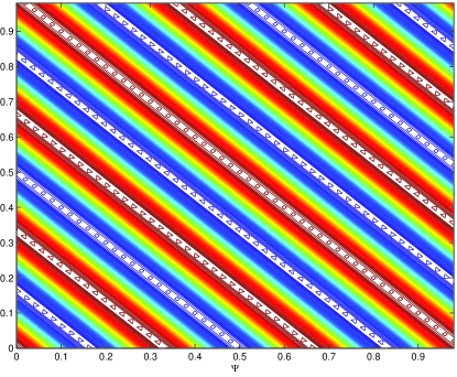
Figure 1: Initial condition: a pure Fourier mode

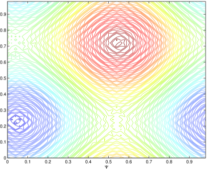
Figure 2: Pattern obtained from the one in Fig.1 after evolution with noise

One sees that the pattern is close to the density of the first Fourier mode. The configuration is not unique. For different runs of the simulation one obtains essentially the same pattern but in different positions on the torus, always close to a first Fourier mode with different phases. This condensation in the first mode, first observed by Kraichnan and Montgomery [36], has been discussed before in the framework of a energy-enstrophy microcanonical measure [14]. However, although we are in a finite $N$ setting, no hint of the microcanonical distribution is apparent. For this first simulation no limitation is put on the dynamical variable, meaning that the dynamical space is $\mathbb{R}^{N^{2}}$. Unique solutions of the measure equation (31) of the type (32) do not apply. However uniqueness of the solution in the $\mathbb{R}^{N^{2}}$ case are also to be expected [32].

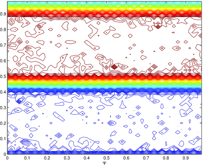
Figure 3: Pattern obtained when the stream function magnitude has an upper bound

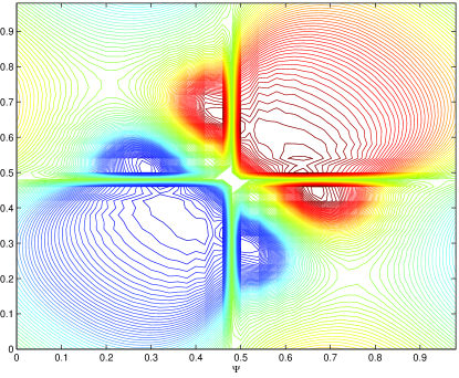
Figure 4: Pattern obtained when the stream function is pinned down to zero at two lines

To explore different boundary conditions in the dynamical space, we considered a case where the values of the stream functions are constrained to be in a box and a case where the stream function is constrained to be zero along two orthogonal lines. We started again from a large mode solution which evolves under noise. The results are shown in Figs.3 and 4. Notice that for simplicity we have considered boundary conditions on the stream function, not on physical velocities which are related to the stream function by Eq.(E1.2a). Boundary conditions on the physical velocities would correspond to boundary conditions on the derivatives of the stream function.

In this paper we have argued for the relevance of stochastically stable measures as the generators of the coherent structures observed in (quasi) two dimensional fluid flows. However most of our results are based on Galerkin approximations of arbitrary but nevertheless finite dimension. In spite of the intuition provided by Eq.(34), the infinite dimension limit characterization remains, of course, an open question.

An alternative approach to the establishment of invariant measures in 2D fluid dynamics has been the Young measure and point vertex model with finite or variable number of vortices [19] [36] [37] [38] [39], which goes back to the pioneering work of Onsager [15]. In this approach, where infinite $N$ limits have been established, Gibbs measures of the vortex model may be identified with coherent structures, however, the selection role of stochastic stability to choose among a basically infinite set of measures is not so clear.

References

- [1] Ya. G. Sinai; Gibbs measures in ergodic theory, Russian Math. Surveys 27 (1972) 21-69.
- [2] R. Bowen; Equilibrium states and the ergodic theory of Anosov diffeomorphisms, Springer Lecture Notes in Math. 470 (1975)
- [3] D. Ruelle; A measure associated with Axiom A attractors, Amer. J. Math. 98 (1976) 619-654.
- [4] D. Ruelle; Chaotic evolution and strange attractors, Cambridge University Press 1989.
- [5] A. Katok and B. Hasselblatt; Introduction to the modern theory of dynamical systems, Cambridge University Press 1995.
- [6] L. Barreira and Y. Pesin; Smooth ergodic theory and nonuniformly hyperbolic dynamics, in ”Handbook of dynamical systems 1B, chapter 2, pp. 57-264”, B. Hasselblatt and A. Katok (Eds.), Elsevier, Amsterdam 2006.
- [7] Y. I. Kifer; On small random perturbations of some smooth dynamical systems, Mat. URSS Izv. 8 (1974) 1083-1107.
- [8] L.-S. Young; Stochastic stability of hyperbolic attractors, Ergodic Theory Dynam. Systems 6 (1986) 311–319.
- [9] Y. I. Kifer; Random Perturbations of Dynamical Systems, Birkhäuser 1988.
- [10] J. F. Alves and M. Viana; Statistical stability for robust classes of maps with non-uniform expansion, Ergodic Theory and Dynamical Systems 22 (2002) 1-32.
- [11] M. Benedicks and M. Viana; Random perturbations and statistical properties of Hénon-like maps, Ann. Inst. H. Poincaré Anal. Non Linéaire 23 (2006) 713–752.
- [12] J. F. Alves, M. Carvalho and J. M. Freitas; Statistical stability for Hénon maps of the Benedicks–Carleson type, Ann. Inst. H. Poincaré Anal. Non Linéaire 27 (2010) 595–637.
- [13] F. Bouchet and A. Venaille; Statistical mechanics of two-dimensional and geophysical flows, Physics Reports 515 (2012) 227-295.
- [14] F. Bouchet and M. Corvellec; Invariant measures of the 2D Euler and Vlasov equations, J. Stat. Mechanics: Theory and Experiment (2010) P08021.
- [15] L. Onsager; Statistical hydrodynamics, Nuovo Cimento supl. 6 (1949) 249-286.
- [16] R. Robert; A maximum entropy principle for two-dimensional perfect fluid dynamics, J. Stat. Phys. 65 (1991) 531-553.
- [17] R. Robert and J. Sommeria; Statistical equilibrium states for two-dimensional flows, J. Fluid Mech. 229 (1991) 291-310.
- [18] E. Caglioti, P. L. Lions, C. Marchioro and M. Pulvirenti; A special class of stationary flows for two-dimensional Euler equations: A statistical mechanics description, Commun. Math. Phys. 174 (1995) 229-260.
- [19] R. Robert; On the statistical mechanics of 2D Euler equation, Commun. Math. Phys. 212 (2000) 245-256.
- [20] S. Albeverio and A. B. Cruzeiro, Global flows with invariant (Gibbs) measures for Euler and Navier-Stokes two dimensional fluids, Commun. Math. Phys. 129 (1990) 431-444.
- [21] F. Cipriano, The two dimensional Euler equation: a statistical study, Commun. Math. Phys. (1999) 139-154.
- [22] H. Airault and H. Ouerdiane; Invariant measure for some differential operators and unitarizing measure for the representation of a Lie group. Examples in finite dimension, Banach Center Publications 96 (2012) 11-34.
- [23] S.Albeverio, M. Ribeiro de Faria and R. Hoegh-Krohn, Stationary measures for the periodic Euler flow in two dimensions, J. Stat. Phys. 20 (1979) 585-595.
- [24] P. J. Morrison; Hamiltonian description of the ideal fluid, Rev. Modern Phys. 70 (1998) 467-521.
- [25] R. Salmon; Lectures on Geophysical Fluid Dynamics, Oxford Univ. Press 1998.
- [26] S. B. Kuksin; The Eulerian limit for 2D statistical hydrodynamics, J. Statist. Phys. 115 (2004) 469–492.
- [27] S. Albeverio and B. Ferrario; Some methods of infinite dimensional analysis in hydrodynamics: An introduction, in ”SPDE in Hydrodynamic: Recent Progress and Prospects”, G. Da Prato and M. Röckner (Eds.), Springer, Berlin 2008.
- [28] M. G. Crandall and P. L.. Lions; Viscosity solutions of Hamilton-Jacobi equations, Trans. Amer. Math. Soc. 277 (1983) 1-42.
- [29] M. G. Crandall, L. C. Evans and P. L. Lions; Some properties of viscosity solutions of Hamilton-Jacobi equations, Trans. Amer. Math. Soc. 282 (1984) 487-502.
- [30] P. L. Lions; Generalized solutions of Hamilton-Jacobi equations, Pitman, London 1982.
- [31] L. C. Evans; Partial differential equations, American Mathematical Society, Providence, R. I. 2010.
- [32] S. Albeverio, V. Bogachev and M. Röckner; On Uniqueness of Invariant Measures for Finite- and Infinite-Dimensional Diffusions, Comm. on Pure and Applied Math. 52 (1999) 325–362.
- [33] A. Friedman; Stochastic differential equations and applications, vol. 1, Academic Press, New York 1975.
- [34] M. G. Crandall and P. L. Lions; Hamilton-Jacobi equations in infinite dimensions, J. Funct. Anal. 62 (1985), 379-396; 65 (1986), 368-405; 68 (1986) 214-247; 90 (1990) 237-283; 97 (1991) 417-465; 125 (1994) 111-148.
- [35] J. P. Bizarro, L. Venâncio and R. Vilela Mendes; A stable semi-implicit algorithm, arXiv:1905.04520.
- [36] R. Kraichnan and D. Montgomery; Two-dimensional turbulence, Rep. Prog. Phys. 43(1980) 547-619.
- [37] G. Benfatto, P. Picco and M. Pulvirenti; On the invariant measures for the two-dimensional Euler flow, J. Statistical Physics 46 (1987) 729-742.
- [38] C. Sire and P.-H. Chavanis; Numerical renormalization group of vortex aggregation in two-dimensional decaying turbulence: The role of three-body interactions, Phys. Rev. E 61 (2000) 6644-6653.
- [39] X. Leoncini, A. Barrat, C. Josserand and S. Villain-Guillot; Offsprings of a point vortex, Eur. Phys. J. B 82 (2011) 173-178.