Spatial modelling with R-INLA: A review

Abstract

Coming up with Bayesian models for spatial data is easy, but performing inference with them can be challenging. Writing fast inference code for a complex spatial model with realistically-sized datasets from scratch is time-consuming, and if changes are made to the model, there is little guarantee that the code performs well. The key advantages of R-INLA are the ease with which complex models can be created and modified, without the need to write complex code, and the speed at which inference can be done even for spatial problems with hundreds of thousands of observations.

R-INLA handles latent Gaussian models, where fixed effects, structured and unstructured Gaussian random effects are combined linearly in a linear predictor, and the elements of the linear predictor are observed through one or more likelihoods. The structured random effects can be both standard areal model such as the Besag and the BYM models, and geostatistical models from a subset of the Matérn Gaussian random fields. In this review, we discuss the large success of spatial modelling with R-INLA and the types of spatial models that can be fitted, we give an overview of recent developments for areal models, and we give an overview of the stochastic partial differential equation (SPDE) approach and some of the ways it can be extended beyond the assumptions of isotropy and separability. In particular, we describe how slight changes to the SPDE approach leads to straight-forward approaches for non-stationary spatial models and non-separable space-time models.

1 Introduction

Spatial modelling is an important, but computationally challenging, statistical field. The main challenge is that the most common modelling tool for capturing spatial dependency, the Gaussian random field (GRF), is hard to use when there is a lot of data. A number of strategies have been proposed for solving this problem, see Heaton et al., (2017) for an up-to-date review. In this paper, we review one particular suite of methods, known as the SPDE approach (stochastic partial differential equations approach). This approach, based on some advanced tools from the theory of stochastic processes, has a computationally efficient implementation in the R-package INLA (R-INLA) (Rue et al.,, 2009, 2017) and has been widely used in practice. The computational efficiency of the R-INLA implementation, as well as the relative simplicity of the interface, has allowed applied spatial researchers to fit a broad range of spatial models to a wide array of applications.

A GRF is completely determined through its mean and covariance (-matrix or -function), and the theory is well understood. Computationally, inference with GRFs naturally results in vector and matrix algebra, for which we can use standard computer libraries. In statistical modelling, we typically use a GRF with a parametrised covariance structure; often a subset of the Matérn covariance family. In this paper, this set of parameters is referred to as hyper-parameters, and the parametrised GRF is referred to as a spatial model component or a spatial random effect.

There are several ways to do inference using the covariance structure of a continuously indexed GRF. The traditional way is to construct the covariance matrix $\boldsymbol{\Sigma}$ for the GRF, based on the observation locations, directly from the covariance function, and then combine it with the covariance matrices for the other model components to create a full covariance matrix for the observations, or for the underlying latent model. This approach can work well for inference with hundreds of locations, but for inference with a hundred thousand locations, the approach is not computationally feasible since computations with $\boldsymbol{\Sigma}$ are too time consuming. Beyond the computational issues, it is challenging to create covariance functions for other geometries such as spheres (the surface of the earth), to introduce non-stationarity in the covariance function, and to extend a spatial covariance function to a non-separable space-time structure.

R-INLA turns the focus from the covariance matrix to the precision matrix $\text{\bf Q}=\boldsymbol{\Sigma}^{-1}$, as it can be shown that several common models with complex covariance structures have sparse precision matrices (Rue and Held,, 2005). Sparse matrices have mostly zeroes, and (most of) the zeroes are not stored in the computer. The sparsity structure of the precision matrix relates to conditional independence between the random variables in the multivariate Gaussian distribution (Rue and Held,, 2005). As we will show in this paper, it is possible to formulate both discretely and continuously indexed spatial models with sparse precision matrices. Let the dimension of a precision matrix for a two-dimensional spatial model with spatial sparsity structure be $n\times n$. Drawing samples, computing the normalising constant, or doing inference, using the sparse precision matrix then require computations of order $\mathcal{O}(n^{3/2})$, compared to the more expensive $\mathcal{O}(n^{2})$ storage and $\mathcal{O}(n^{3})$ computations required for the corresponding dense covariance matrix. Applications with hundreds of thousand of locations are then feasible, and applications with a few thousand observations can be analysed with the click of a button.

In R-INLA we achieve the desired spatial sparsity structure for the precision matrix of the continuously indexed GRF by using the SPDE approach (Lindgren et al.,, 2011). Instead of constructing a discrete model for the GRF on a set of locations or grid cells by using a covariance function, we construct a continuously indexed approximation of the GRF by using a continuous model—an SPDE—that is defined on the entire study area. For example, the Matérn covariance function is given by

$$c(s_{1},s_{2})=\sigma^{2}\frac{2^{1-\nu}}{\Gamma(\nu)}(\sqrt{8\nu}||s_{1}-s_{2}||/\rho)K_{\nu}(\sqrt{8\nu}||s_{1}-s_{2}||/\rho),$$ (1)

where $\Gamma$ is the Gamma function, $\rho$ is the spatial distance at which correlation is approximately $0.13$, $\sigma$ is the marginal standard deviation, $\nu$ is the smoothness parameter, and $K_{\nu}$ is the modified Bessel function of the second kind, order $\nu$. The parameters of this covariance function have clear physical meanings, but the covariance function can only be used directly for small problems.

We use the result by Whittle, (1954, 1963) that shows that a stationary solution of the SPDE

$$\left(\kappa^{2}-\Delta\right)^{\alpha/2}(\tau u(\boldsymbol{s}))=\mathcal{W}(\boldsymbol{s}),\quad s\in\mathbb{R}^{d},$$ (2)

has a Matérn covariance function, where $\kappa>0,\tau>0$, $\alpha>d/2$, $\Delta=\sum_{i}\partial^{2}/\partial s_{i}^{2}$ is the Laplacian, and $\mathcal{W}$ is standard Gaussian white noise. The parameters used in Equation 2 are the standard parameters for the SPDE and are different from the ones in Equation (1), but there is a one-to-one correspondence between them. The advantage of the parameters of the Matérn covariance function is that they have direct physical interpretations and the advantage of the parameters of the SPDE is that they make it simpler to write the SPDE. See Lindgren et al., (2011) for the formulas describing how to convert between the parametrisations. Based on this SPDE, restricted to a bounded domain with appropriate boundary conditions, we can construct a continuously indexed approximation to the solution that approximately has the Matérn covariance structure. We can also use the one-to-one correspondence between the parameters of the Matérn covariance function and the parameters of the SPDE, to estimate the model using the computationally efficient approximation, and interpret the results through the well-known Matérn covariance function. The use of a finite element method (FEM) for constructing the approximate solution on the bounded domain allows for boundaries made up of complex polygons and for different fidelity of the discretisation in different areas. For integer $\alpha$ values, the continuous domain SPDE solutions are Markovian, which is reflected in sparse precision matrices for the discrete approximations. For other $\alpha$ values, sparse approximations can yield close correspondences.

We highlight the main advantages of the SPDE approach.

1. The dimension of the finite-dimensional Gaussian approximation to the solution of the SPDE only depends on the desired resolution and is invariant to the number of observations.

2. The non-vanishing spatial correlations of the approximate solution are represented by a Markovian structure on the precision matrix (inverse covariance matrix) where only close neighbours are non-zero. We present this idea in detail in Section 4.

3. The non-zero structure of the precision matrix is invariant to the spatial correlation range, determined by $\kappa$, of the approximate solution. The number of non-zero neighbours does however depend on the smoothness $\nu$.

4. Small changes to the differential operator in the SPDE leads to models on manifolds, and non-stationary and non-separable models, see Section 6. If the operator is changed, but the exponent $\alpha/2$ is the same, the process of computing the matrices is the same as for the stationary models, and the precision matrices are automatically sparse and positive definite as long as the SPDE is well-defined.

The speed-up we get by running our spatial models in R-INLA, the ease of using the spatial model together with other model components, and the ability to use a wide variety of observation likelihoods for the latent process makes R-INLA a very useful tool for applied statistical modelling. Models that used to be too complex to be fitted in the Bayesian framework are now possible to run in a day. And, perhaps more importantly, models we could previously run in a day can now be run in an even shorter time, enabling researchers to fit several different models, to understand the data, to investigate prior sensitivity, to investigate sensitivity to the choice of observation likelihood, to run bootstrap analyses, and to perform cross-validation and other predictive comparisons. Another improvement is in reproducibility, and code checking by other researchers, as code published together with papers can often be run in an hour.

There are several high impact applications using spatial models in R-INLA; in the journal The Lancet Noor et al., (2014) performed a space-time analysis of transmission intensity of malaria and Golding et al., (2017) modeled under-five mortality and neo-natal mortality in multiple countries with separable space-time models for different age groups; in the journal Science Jousimo et al., (2014) studied the effects of fragmentation on infectious disease dynamics; in the journal Nature Bhatt et al., (2015) analysed the effect of the various efforts to to control malaria in Africa. R-INLA’s spatial capabilities were also a key tool used by Shaddick et al., (2018) to produce the global estimates of ambient exposure to ultra-fine particulate matter of less than 2.5$\mu$m in diameter, known as PM_2.5, that were used in both the 2016 Global Burden of Disease study (Gakidou et al.,, 2017) and the World Health Organization’s assessment of health risk due to ambient air pollution (World Health Organization,, 2016).

A collection of some recent examples of spatial applications with the R-INLA software, intended as a source of inspiration for the reader, follows; environmental risk factors to liver Fluke in cattle (Innocent et al.,, 2017) using a spatial random effect to account for regional residual effects; modelling fish populations that are recovering (Boudreau et al.,, 2017) with a separable space-time model; mapping gender-disaggregated development indicators (Bosco et al.,, 2017) using a spatial model for the residual structure; environmental mapping of soil (Huang et al.,, 2017) comparing a spatial model in R-INLA with “REML-LMM”; changes in fish distributions (Thorson et al.,, 2017); febrile illness in children (Dalrymple et al.,, 2017); dengue disease in Malaysia (Naeeim and Rahman,, 2017); modelling pancreatic cancer mortality in Spain using a spatial gender-age-period-cohort model (Etxeberria et al.,, 2017); soil properties in forest (Beguin et al.,, 2017) comparing spatial and non-spatial approaches; ethanol and gasoline pricing (Laurini,, 2017) using a separable space-time model; fish diversity (Fonseca et al.,, 2017) using a spatial GRF to account for unmeasured covariates; a spatial model of unemployment (Pereira et al.,, 2017); distance sampling of blue whales (Yuan et al.,, 2017) using a likelihood for point processes; settlement patterns and reproductive success of prey (Morosinotto et al.,, 2017); cortical surface fMRI data (Mejia et al.,, 2017) computing probabilistic activation regions; distribution and drivers of bird species richness (Dyer et al.,, 2017) with a global model, and comparing several different likelihoods; socio-environmental factors in influenza-like illness (Lee et al.,, 2017); global distributions of Lygodium microphyllum under projected climate warming (Humphreys et al.,, 2017) using a spatial model on the globe; logging and hunting impacts on large animals (Roopsind et al.,, 2017); socio demographic and geographic impact of HPV vaccination (Rutten et al.,, 2017); a combined analysis of point and area level data (Moraga et al.,, 2017); probabilistic prediction of wind power (Lenzi et al.,, 2017); animal tuberculosis (Gortázar et al.,, 2017); polio-virus eradication in Pakistan (Mercer et al.,, 2017) with a Poisson hurdle model; detecting local overfishing (Carson et al.,, 2017) from the posterior spatial effect; joint modelling of presence-absence and abundance of hake Paradinas et al., (2017); topsoil metals and cancer mortality (López-Abente et al.,, 2017) with spatially misaligned data; applications in spatial econometrics (Bivand et al.,, 2014; Gómez-Rubio et al.,, 2015, 2014); modeling landslides as point processes (Lombardo et al.,, 2018); comparing avian influenza virus in Vietnamese live bird markets (Mellor et al.,, 2018) and predicting extreme rainfall events in space and time (Opitz et al.,, 2018).

This paper is meant to give an understanding of the possibilities and limitations for spatial models in R-INLA. The main focus is on the continuously indexed spatial models defined through the SPDE approach, but we provide a brief description of areal models and recent developments for them. We do not give a detailed introduction of R-INLA, which is found in Rue et al., (2017), or how to program spatial models in R-INLA, which is found in Lindgren and Rue, (2015); Blangiardo and Cameletti, (2015); Bivand et al., (2015); Gómez-Rubio et al., (2014); Krainski et al., (2017) and at www.r-inla.org. After giving some necessary background in Section 2, we start with areal models in Section 3 and proceed to discuss continuously indexed models and the SPDE approach in Section 4. In Section 5 we discuss how the spatial random effects together with general features of R-INLA makes it possible to create a wide variety of models ranging from simple Gaussian geostatistical models to spatial point process models. In Section 6 we show how we can loosen the restrictions of isotropy and Gaussianity for the spatial effect within the SPDE approach, and we end with a discussion on the road into the future in Section 8.

2 Notation and background on R-INLA

In this section we give a brief overview of the parts central to spatial models from the R-INLA review paper (Rue et al.,, 2017). We use boldface symbols ($\boldsymbol{u}$) to denote the discrete (matrix or vector) objects, while indexed lowercase ($u_{i}$) denotes the elements in the matrices and vectors, and the ordinary lowercase ($u$) denotes a continuous spatial field ($u(\boldsymbol{s})$) or a function.

The data $y_{i}$ are conditionally independent given the (linear) predictor $\eta_{i}$

$$y_{i}|\eta_{i},\boldsymbol{\theta}_{0}\sim\pi(y_{i}|\eta_{i},\boldsymbol{\theta}_{0}),$$

where different $y_{i}$ can have different observation likelihoods. The vector $\boldsymbol{\theta}_{0}$ is the first set of hyper-parameters, and are usually the scale and shape parameters of the chosen likelihood(s).

The linear predictor $\boldsymbol{\eta}$ is modelled by a sum of fixed and random effects

$$\boldsymbol{\eta}=\text{\bf A}_{1}\boldsymbol{u}_{1}+...+\text{\bf A}_{k}\boldsymbol{u}_{k}+...$$

where $k$ signifies that this is component number $k$, but we will suppress the $k$ for notational convenience. The random vector $u$ has a Gaussian prior

$$\boldsymbol{u}|\boldsymbol{\theta}_{k}\sim\mathcal{N}(\text{\bf 0},\text{\bf Q}^{-1})$$

where the precision matrix Q depends on the hyper-parameters $\boldsymbol{\theta}_{k}$ for this random effect. There must be a constant sparsity structure for Q, across all of $\boldsymbol{\theta}_{k}$’s values, and we call this the graph (the non-sparse elements in Q can be zero for some values of $\boldsymbol{\theta}_{k}$). The projection matrix A is a known sparse matrix, often just a matrix of 0’s and 1’s signifying which entry of the random effect $\boldsymbol{u}$ is used for the observation $i$. For example, if both the first and seventh observation in space is at the same location, the first and seventh row of A are equal and have a 1 in the column corresponding to that location and 0’s otherwise. We detail several different choices of models for $u$ in this review, and we describe the A-matrix for SPDE models in Section 4.5.

The dimension of the hyper-parameters

$$\boldsymbol{\theta}=(\boldsymbol{\theta}_{0},\boldsymbol{\theta}_{1},...,\boldsymbol{\theta}_{K})$$

should not be too large, meaning less than 20 and preferably around 5, because the exploration of the posterior of $\boldsymbol{\theta}$ is expensive. One evaluation of $\pi(\boldsymbol{\theta}|\boldsymbol{y})$ requires factorising the precision matrix and approximating the posterior contribution of the likelihood by a Laplace approximation.

Additionally, the posterior of the hyper-parameters should be unimodal and not too different from a multivariate Gaussian. To satisfy this, we depend on good parametrisations. For example, the posterior for the marginal standard deviation $\sigma$ is usually skewed and has a heavy tail, while the posterior of $\log(\sigma)$ is well-behaved.

In this framework there is no difference between 1-dimensional models, e.g. non-linear covariate effects, and 2-dimensional spatial models, or 3-dimensional space-time models. The inla()-call itself does not know that we are fitting a spatial model, it only knows that we have a precision matrix with a certain graph and that the supplied A-matrix connects the precision matrix to $\eta_{i}$. We know that this precision matrix represents a spatial correlation structure and that the supplied A-matrix projects from the 1-dimensional vector $\boldsymbol{s}$ of spatial indices to the two dimensional spatial (longitude, latitude) description. The work we need to do, to create a spatial model in R-INLA, is constructing a “good” precision matrix and A-matrix, according to our understanding of “good”.

For applications with space-time data, the simplest interaction models are the separable models, defined through Kronecker products,

$$\text{\bf Q}_{\mathrm{spacetime}}=\text{\bf Q}_{\mathrm{time}}\otimes\text{\bf Q}_{\mathrm{space}}.$$

Kronecker models are implemented as a general feature in R-INLA, where $\text{\bf Q}_{\mathrm{space}}$ can be any spatial model, including the model in Section 3, and $\text{\bf Q}_{\mathrm{time}}$ can be selected from a small collection of temporal models, including random walk of order 1 and 2, autoregressive of order 1, and iid models (replicates). The ability to mix and match model components to create the desired space-time model is of great interest, and means that whenever we implement a spatial model in R-INLA, we get all these space-time models with almost no additional work.

The standard approach for making predictions is to add “fake data rows” containing the covariates/location we wish to predict, but with NA in place of observed data. This can be computationally inefficient for spatial models since it is computationally equivalent to fitting extra observations. For spatial predictions where there may be $10^{5}$ prediction locations this may lead to long computation times (Huang et al.,, 2017) and while it can be reduced somewhat by re-running the model multiple times with disjoint subsets of the desired prediction locations (Poggio et al.,, 2016), a better approach is to use i.i.d. samples from the joint posterior. Fuglstad and Beguin, (2018) show that similar prediction results can be obtained in 11 minutes using posterior samples as takes 24 hours with the standard approach with NA observations (Huang et al.,, 2017).

2.1 The Laplace approximation

The Laplace approximation is an essential component of INLA, allowing for fast computations across a wide range of likelihoods and link functions. If the likelihood is Gaussian, i.e. $\boldsymbol{y}\sim\mathcal{N}(\boldsymbol{\eta},\boldsymbol{\theta}_{0})$, the unnormalised posterior density of $\pi(\boldsymbol{\theta}|\boldsymbol{y})$ can be computed exactly,

$$\pi(\boldsymbol{\theta}|\boldsymbol{y})\propto\frac{\pi(\boldsymbol{y}|\boldsymbol{\eta}=\boldsymbol{0},\boldsymbol{\theta})\pi(\boldsymbol{\eta}=0|\boldsymbol{\theta})}{\pi(\boldsymbol{\eta}=\boldsymbol{0}|\boldsymbol{y},\boldsymbol{\theta})}\pi(\boldsymbol{\theta}).$$ (3)

For non-Gaussian likelihoods, we compute an approximation of this equation. The Laplace approximation does not approximate the likelihood $\pi(\boldsymbol{y}|\boldsymbol{\eta},\boldsymbol{\theta})$, but the conditional distribution $\pi(\boldsymbol{\eta}|\boldsymbol{y},\boldsymbol{\theta})$. For example, for a Poisson likelihood, a Gaussian prior on $\eta_{i}$, and observing $y_{i}=1$, the $\pi(y_{i}|\eta_{i},\boldsymbol{\theta})$ cannot be approximated by a Gaussian, but $\pi(\eta_{i}|y_{i},\boldsymbol{\theta})$ can. The Laplace approximation is a quadratic approximation of the log-density around the posterior mode of $\boldsymbol{\eta}|\boldsymbol{\theta}$, which is found by iteration. This posterior mode is subsituted for $\boldsymbol{0}$ in equation (3) to compute $\pi(\boldsymbol{\theta}|\boldsymbol{y})$.

The posterior for $\boldsymbol{\eta}$ and all other latent variables are computed by numerical integration over $\pi(\boldsymbol{\theta}|\boldsymbol{y})$, using an additional Laplace approximation, see Rue et al., (2017) Section 3.2. The option int.strategy = ’eb’ in R-INLA specifies that this integration is only done with a single evaluation at the posterior mode of $\boldsymbol{\theta}$, and is commonly used for very computationally intensive models. The option int.strategy = ’ccd’ is the default for $\boldsymbol{\theta}$ of dimension larger than 2, and allows for computing the posterior of $\eta$ when the dimension of $\theta$ is large (but less than 20). The option int.strategy = ’grid’ can be used to create a grid of integration points over $\boldsymbol{\theta}$, and the user can further configure this grid to gain greater accuracy when representing the posterior. However, grids are afflicted by the curse of dimensionality and appropriate only for low-dimensional spaces.

When the model includes a spatial model component $u$, the posterior marginals for $u$ are computed by R-INLA. This collection of marginals is rarely used directly, e.g. it is almost impossible to plot the entire collection. From these marginals, R-INLA computes quantiles and the marginal standard deviation. The spatially varying posterior marginal standard deviation is often used as a proxy for spatial uncertainty. In applications with a non-linear link function, however, the standard deviation is not a good proxy for uncertainty, and one can instead use the upper and lower quantiles, or the inter-quartile range.

3 Areal models and other discretely indexed models

In this review we separate the models into discretely and continuously indexed models. A discretely indexed model (component) $u$ has a finite set of indices $i$, and it is not clear how to extend the model to other indices, i.e. other ‘locations’, ’areas’ or ‘covariate values’. Discretely indexed spatial models fit into the standard framework of R-INLA and there are several good introductions towards their implementation, see for example Schrödle and Held, 2011a ; Schrödle and Held, 2011b ; Schrödle et al., (2012); Ugarte et al., (2014) or Blangiardo and Cameletti, (2015, Section 6.1-6.4). One of the most well known discrete spatial model components is what we refer to as the Besag model (Besag et al.,, 1991)—in honour of the statistician J.E. Besag—commonly known as the “CAR” or “iCAR” model. We use the name conditionally autoregressive (CAR) model for any multivariate Gaussian model that is built up through conditional distributions, so, in our terminology, the Besag model is a particular example of a CAR model.

3.1 The Besag model

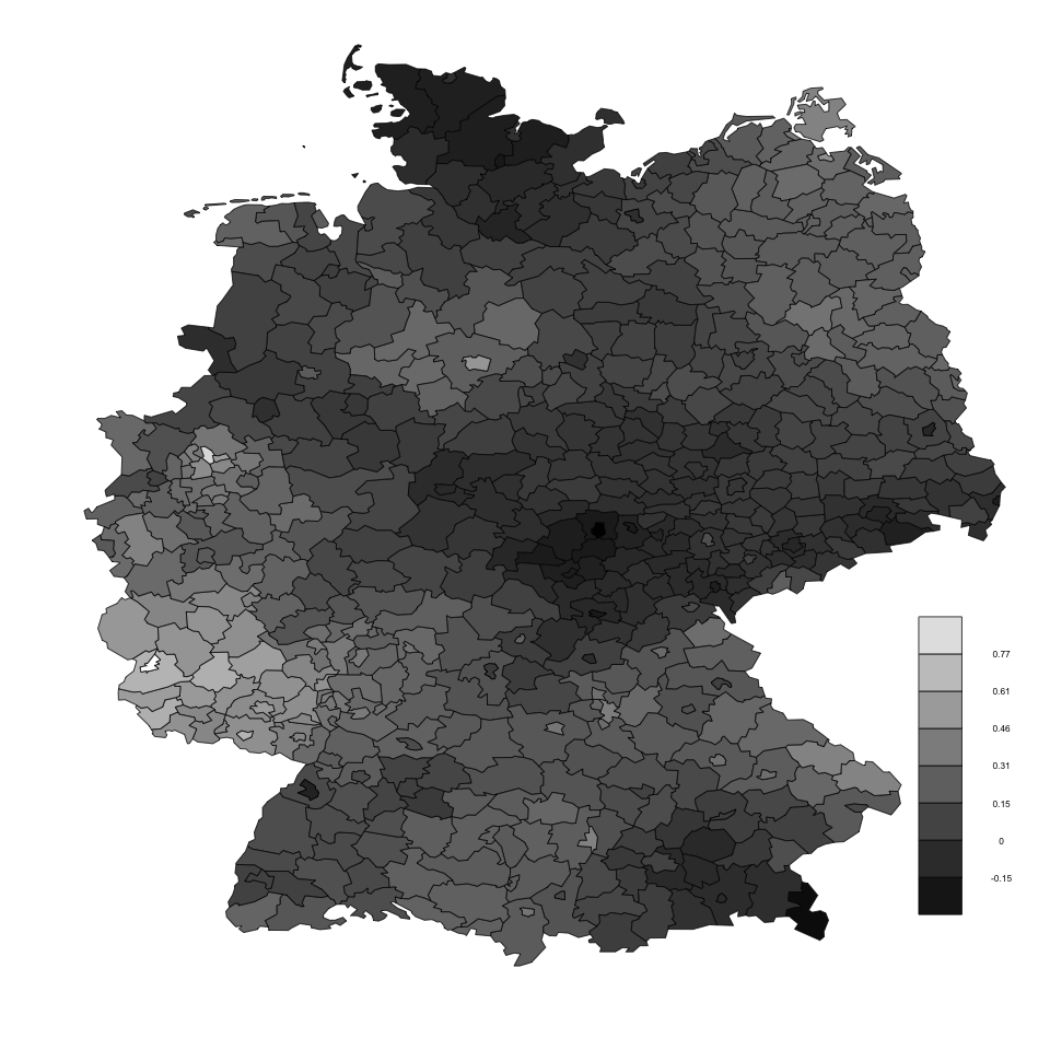
The Besag model models the values $u_{i}$ on a collection of regions $i=1,\ldots,n$, see Figure 1, conditionally on the neighbouring regions. Two regions are usually defined as neighbours when the share a common border.

Figure 1: Besag model. The left plot shows an example dataset over regions in Germany, and the right plot shows the sparse precision matrix Q.

The conditional distribution for $u_{i}$ is

$$u_{i}|\boldsymbol{u}_{-i},\tau_{u}\sim\mathcal{N}\left(\frac{1}{d_{i}}\sum_{j\sim i}u_{j},\frac{1}{d_{i}}\frac{1}{\tau_{u}}\right),$$

where $j\sim i$ denotes that $i$ and $j$ are neighbouring areas, and $d_{i}$ is the number of neighbours. The joint distribution is given by

$$\boldsymbol{u}|\tau_{u}\sim\mathcal{N}\left(0,\frac{1}{\tau_{u}}\text{\bf Q}^{-1}\right),$$

where Q denotes the structure matrix and is defined as

$$Q_{i,j}=\left\{\begin{tabular}[]{ll}$d_{i},$&$i=j$\\ -1,&$i\sim j$\\ \end{tabular}\right.,$$ (6)

and $0$ otherwise. This structure matrix directly defines the neighbourhood structure and is sparse per definition, having $\mathcal{O}(n)$ non-zero elements. Of note, a weighted Besag model, where positive weights are incorporated for each pair of neighbouring regions, can be defined analogously, see Rue and Held, (2005, Section 3.3.2). There are different ways to provide the neighbourhood structure given by (6) to R-INLA: 1) Through an ASCII file; 2) through a symmetric adjacency matrix of dimension $n\times n$; 3) by extracting the structure directly from the shapefile using the R-packages maptools (Bivand and Lewin-Koh,, 2017) and spdep (Bivand and Piras,, 2015; Bivand et al., 2013a, ). We refer to Blangiardo and Cameletti, (2015, Section 6.1) for implementation details of the Besag model in R-INLA.

It is generally recommended to combine the Besag model with an additional unstructured random effect $v_{i}\mid\tau_{v}\sim\mathcal{N}(0,\tau_{v}^{-1})$ per region $i=1,\ldots,n$. The resulting spatial model $u_{i}+v_{i}$ for $i=1,\ldots,n$ is often termed BYM model following the initials of the authors who proposed it, Besag, J., York, J., and Mollie, A. (Besag et al.,, 1991).

3.2 Prior specification for the Besag model

The Besag model penalises local deviation from a constant level in the case where all regions are connected. The prior on the hyper-parameter(s) will control this local deviation, i.e. the amount of smoothing, but unfortunately its specification is not straightforward, see for example Bernardinelli et al., (1995); Wakefield, (2007). One challenge is that $\tau_{u}$ is not directly interpretable, as it depends on the underlying graph.

The first step to interpreting $\tau_{u}$ is making the Besag model proper, by constraining the model to sum to zero (on each disconnected set). The second step is to make the interpretation of $\tau_{u}$ independent of the total number of regions and the set of edges (connections between neighbours). To see how unstable the definition of $\tau_{u}$ is consider the marginal standard deviation

$$\text{Sd}(u_{i})=\frac{\sqrt{{\text{\bf Q}}^{-}_{ii}}}{\sqrt{\tau_{u}}}\quad\text{for }i\in 1,\ldots,n,$$

whereby $\text{\bf Q}^{-}$ denotes the generalised inverse of Q. The marginal standard deviation is not constant over $i$, and any maximum or average value depends heavily on the size $n$ of the model. Sørbye and Rue, (2014) propose to scale Q such that the geometric mean of the marginal variances of u does not depend on $n$ or on the connectivity structure. This implies that $\tau_{u}$ represents the precision of the (marginal) deviation from a constant level, independently of the underlying graph, facilitating prior specification. Freni-Sterrantino et al., (2018) recommend scaling each connected component independently, and give advice for how to define the Besag model for a general graph.

Further, we can specify the joint prior for the Besag and iid components by reparametrising the BYM model as

$$\mathbf{b}=\frac{1}{\sqrt{\tau}}\left(\sqrt{1-w}\boldsymbol{v}+\sqrt{w}\boldsymbol{u}^{\star}\right)$$ (7)

containing a scaled Besag component $\boldsymbol{u}^{\star}$. This model, called BYM2 in R-INLA, explicitly models the distribution of variance between two components; the structured scaled effects $\boldsymbol{u}^{\star}$ and the unstructured effects $\boldsymbol{v}$. For details on how to choose sensible priors for $\tau$ and $w$ in the BYM2 model we refer to Appendix A.1.

3.3 Discretely indexed models

The Besag model is the most commonly used spatial discretely indexed model. Any other discretely indexed model $u\sim\mathcal{N}(0,\tau^{-1}Q^{-1})$ is implemented as generic0. Prior specification for this $\tau$ can be done in a similar manner to what we do for the Besag. Discretely indexed models where the precision matrix depends on hyper-parameters can be implemented using rgeneric, such as the model proposed by Dean et al., (2001), and the Leroux model (Leroux et al.,, 2000). However, in these cases prior specification depends on the model in question, and we are often not able to give a recommendation.

In the research done by the R-INLA group there is a general movement away from discretely indexed models, towards continuously indexed models. The discretely indexed models are typically used because they offer a simple and computationally efficient way to achieve spatial smoothing. However, these models ignore sub-regional variation, do not account for differing region sizes or how much boundary is shared between each pair of regions, and have difficulties handling geographic boundaries that are channging in time. To overcome these issues, one can model the data at a very fine resolution using continuously indexed models, and include the spatially aggregated observations as integrals over the regions. However, this is challenging for non-linear link functions, and when we model, for example, risk we require fine-scale information about the spatially varying population-at-risk. Also, in some situations the areas are themselves relevant for modelling the underlying process (e.g. in Lombardo et al., (2018)). Because of this, we expect that discretely indexed models will continue to be an important part of the R-INLA package going forwards.

3.4 Space-time models

Extending spatial model components to space-time interaction components is straightforward using R-INLA, see Section 2, and thus the Besag model can be extended to a space-time interaction model. Knorr-Held, (2000) proposed four interaction types where the structure matrix results as a Kronecker product of the structure matrices of the effects supposed to interact. The resulting model can be defined in R-INLA either as a user-defined rgeneric model or by making use of the Kronecker structure, see Riebler et al., (2012); Blangiardo et al., (2013) for code snippets. The challenge of these interaction models is the possibly large number of linear constraints required to ensure identifiability of all model parameters (Schrödle and Held, 2011b, ; Papoila et al.,, 2014; Goicoa et al.,, 2017). Since the computational cost of constraints in R-INLA is $\mathcal{O}(nk^{2})$ for $k$ constraints and $n$ space-time points, a large number of constraints will result in models that are no longer computationally feasible. Krainski, (2018) proposes an alternative formulation avoiding linear constraints entirely by trading them for computationally cheaper linear combinations to solve identifiability issues. Future work aims at defining those linear combinations automatically whenever an R-INLA user uses one of the standard interaction models.

4 Continuously indexed models

The Matérn covariance function shown in Equation (1) is one of the most important and most frequently used covariance functions for spatial models. In this section we discuss how the Matérn model is represented in R-INLA through the SPDE approach.

4.1 Representing a continuously indexed spatial model in R-INLA

Let $u(\boldsymbol{s})$ be a continuously indexed GRF and assume that observations $y(\boldsymbol{s}_{k})$ are made of a physical process that is described by

$$y(\boldsymbol{s}_{k})=X(\boldsymbol{s}_{k})\beta+u(\boldsymbol{s}_{k})+\epsilon_{k},$$ (8)

where $X$ is a spatially varying covariate, $\beta$ is the coefficient of the effect of the covariate, $\boldsymbol{s}_{k}$ is the observation location, and $\epsilon_{k}$ is Gaussian noise that is i.i.d. for the observations. The first part of the model, $X(\boldsymbol{s}_{k})\beta+u(\boldsymbol{s}_{k})$, is the spatially varying signal of interest, but it cannot be directly observed due to the noise $\epsilon_{k}$ associated with the observation process. More complex observational processes can be constructed using a link function and a non-Gaussian likelihood as we explain in Section 5.

The question is now how to represent the covariance structure of $u(\boldsymbol{s})$ in a computationally efficient way for performing inference with the above model in R-INLA. For now, assume that the set of observations form a square grid. The vector $\boldsymbol{u}$, which consists of the variables stacked column-wise, has a multivariate Gaussian distribution with a covariance matrix $\boldsymbol{\Sigma}$ computed from the covariance function. In R-INLA, it is represented as

$$\boldsymbol{u}\sim\mathcal{N}(\text{\bf 0},\text{\bf Q}^{-1}),$$

where $\text{\bf Q}=\boldsymbol{\Sigma}^{-1}$. However, the precision matrix Q is in general not sparse, which makes computations infeasible for large datasets.

Conditional Autoregressive (CAR) and Simultaneous Autoregressive (SAR) models (Besag,, 1974) have sparse precision matrices by construction, and a first attempt would be to approximate the desired covariance structure for the gridded observations by such models. One way to find a CAR to represent the GRF we want is to make a long list of different spatial CAR models and investigate what covariance functions they approximate. Along this line, Rue and Tjelmeland, (2002) assumed that the parameters in the precision matrix for grid cells more than $k$ steps apart in at least one direction was zero, and parametrised the rest of the precision matrix. Assuming translational and rotational invariance (90 degree rotations), there are only a few parameters that need to be inferred; for $k=3$ there are 6 parameters.

This approach to parametrise CAR models has several issues. Any parametrisation of the CAR model must give positive definite precision matrices, but the space of valid parameters does not have an intuitive shape (see e.g. Rue and Held, (2005) Section 2.7.1). One needs to map the parameters of the CAR model to interpretable parameters, such as the spatial range parameter, in a continuous way, but this is difficult and may have to be done separately for each application. Further, it is necessary to investigate for which parts of the parameter space the approximation to the continuous model is sufficiently good, and, setting priors on the CAR parameters necessitates dealing with the boundaries between proper and intrinsic models. Perhaps most importantly, generalising to irregular observations, to the sphere, or to non-stationary covariance functions, is notoriously difficult as it exacerbates all these issues.

The key to solving these issues is to stop focusing on the parameters of the CAR model, and instead focus on the continuous representation of the GRF through an SPDE, letting the CAR parameters be a side-effect of computing a continuous approximation to the continuously indexed GRF. The SPDE approach produces precision matrices that enjoy the good computational properties of the CAR models and is valid for any set of observation locations. Generalisation, interpretable parameters, and stability of the CAR structure, can then be investigated based on the continuous interpretation of the SPDE.

4.2 Discretising a differential operator

In this section we consider functions on $\mathbb{R}^{2}$ and denote the coordinates of locations $\boldsymbol{s}\in\mathbb{R}^{2}$ by $x$ and $y$. A differential operator $\mathcal{L}$ is a function of functions, taking as input a surface $u(\boldsymbol{s})$ and gives as output another surface $\mathcal{L}(u)(\boldsymbol{s})$, for example

$$\mathcal{L}_{1}(u)=\kappa^{2}u-\nabla\cdot\nabla u,$$

where $\kappa>0$, $\nabla=\left[\frac{\partial u}{\partial x},\frac{\partial u}{\partial y}\right]$ is the gradient, and $\Delta=\nabla\cdot\nabla=\partial^{2}/\partial x^{2}+\partial^{2}/\partial y^{2}$ is the Laplacian. Using $\mathcal{L}_{1}$ on the function $u(x,y)=\sin(2x)+y$ produces $L(u)(x,y)=\kappa^{2}\sin(2x)+\kappa^{2}y+4\sin(2x)$.

When $u$ is defined on a grid, we can approximate the continuously indexed $u$ by a vector $\boldsymbol{u}$ consisting of the values of $u$ on the grid stacked column-wise. For this discrete representation, the operator $\mathcal{L}$ has a corresponding discretised version that can be written as a matrix L, so that $\text{\bf L}\boldsymbol{u}$ produces approximately the same values as if $\mathcal{L}u$ were evaluated at the grid. There are many ways to discretise operators, giving many different possibilities for L-matrices. One discretisation approach is the use of finite differences on a regular grid, allowing the CAR to be visualised by a computational stencil, see Appendix A.2.

4.3 Constructing a continuously indexed approximation

Discretised operators based on finite differences for SPDEs can be used to construct models that fit within the R-INLA framework. However, finite difference methods give discretely indexed approximations, having several disadvantages, including being difficult to extend to irregular locations, non-rectangular grids or sparsely observed grids. Therefore, it is more natural to follow the numerics literature on partial differential equations (PDEs) and instead approximate a solution of the SPDE as a sum of finitely many basis functions. We now introduce a more complex discretisation method that will be used to construct the approximately Matérn GRFs based on the SPDE in Equation (2).

Let $\{\phi_{j}(\boldsymbol{s})\}$ be a set of basis functions, then any permissible function $u(\boldsymbol{s})$ is on the form

$$u(\boldsymbol{s})=\sum_{j=1}^{J}a_{j}\phi_{j}(\boldsymbol{s}),$$ (9)

where $a_{j}$ are real-valued coefficients for the basis functions. The idea is to discretise the differential operator $\mathcal{L}$ to a matrix L on the coefficients $a_{j}$, instead of with respect to a grid. In this setting,

$$\mathcal{L}\left(\sum_{j=1}^{J}a_{j}\phi_{j}(\boldsymbol{s})\right)\approx\sum_{j=1}^{J}b_{j}\phi_{j}(\boldsymbol{s}),$$ (10)

where $(b_{1},\ldots,b_{J})=\text{\bf L}(a_{1},\ldots,a_{J})$. This idea can be made precise in terms of bases, operators and projections on Hilbert spaces. One of the main advantages of using a basis of continuous functions is that any solution is a continuous function, hence the solution is defined everywhere and can be evaluated at any desired location without interpolation techniques. This is what we call a “continuously indexed approximation”. The main difficulty with this approach is to find a good basis $\left\{\phi_{j}\right\}$, with a computationally efficient (sparse) discretisation matrix L.

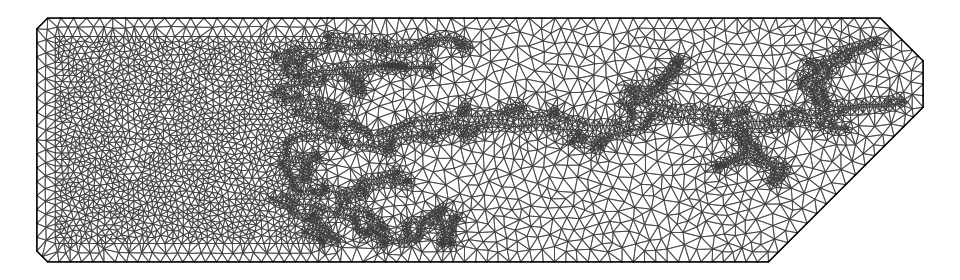
The approach that was chosen in Lindgren et al., (2011) is known as the finite element method (FEM) with linear elements, see e.g. Brenner and Scott, (2007), which is an excellent practical computational tool. In the FEM, the grid is replaced by a mesh, see Figure 2. In our framework, the mesh is composed of triangles and covers the entire domain, and a bit more to account for boundary conditions. The basis functions, $\phi(\boldsymbol{s})$ in equation (9), known as linear elements, or hat-functions, are constructed based on this mesh. The vertices of the triangles are called nodes, and at each node $j$, $\phi_{j}=1$, at any other node $\phi_{j}=0$, and $\phi_{j}$ on the triangles are given by linear interpolation. Any piecewise linear—with respect to the mesh—function is then a linear sum of these elements. The theory of the FEM is well-established, meaning we can re-use results in the literature to compute the matrix L, and, given that we follow established recommendations for how to define the mesh and the elements, we expect no unwelcome surprises. Additionally, since the mesh is a collection of triangles, we can have complicated polygons as boundaries to our mesh.

Figure 2: An example mesh, constructed for the Norwegian fjord “Sognefjorden”.

4.4 R-INLA implementation of the Matérn fields

The construction of the mesh for a specific application is an involved process, implemented as inla.mesh.2d, and documented in R-INLA and in the tutorials at www.r-inla.org. The A-matrix connects the GRF-on-the-mesh to the GRF-on-the-data, $A_{i,j}=\phi_{j}(s_{i})$, and is computed using
inla.spde.make.A(mesh, observation.locations). When smoothing spatial data, with no covariates, the INLA-call is simple, the A-matrix is included in the control.predictor input. However, if there are several other model components or a space-time model component, keeping track of all the different A-matrices is challenging, and we developed the inla.stack interface to handle all these matrix operations in a general way (Lindgren and Rue,, 2015). In Section 7 we will mention some recent efforts to further simplify the specification of these models.

After the mesh in constructed, the R-INLA model inla.spde2.pcmatern implements the Matérn GRFs, and is described in Lindgren et al., (2011) Section 2.3, and Lindgren and Rue, (2015) Section 1.1. The stationary Matérn family is represented by an approximate solution of the SPDE

$$\left(\kappa^{2}+\nabla\cdot\nabla\right)^{\alpha/2}(\tau u(\boldsymbol{s}))=\mathcal{W}(\boldsymbol{s}),\qquad s\in\mathcal{D}\subset\mathbb{R}^{d},$$ (11)

where $\mathcal{D}$ is a polygonal domain (i.e. we can make a mesh on $\mathcal{D}$), $\alpha$ is an integer, and we use Neumann boundary conditions. The boundary conditions are not discussed in this paper, but warrants that the mesh covers a larger area than the observations, see Lindgren et al., (2011) Appendix A.4. This SPDE results in smoothness $\nu=\alpha-d/2$. The basic FEM matrices are set up as

$$C_{i,i} =\langle\phi_{i},1\rangle$$ (12)

$$G_{i,j} =\langle\nabla\phi_{i},\nabla\phi_{j}\rangle$$ (13)

K $$=\kappa^{2}\text{\bf C}+\text{\bf G},$$ (14)

where the other elements of C are zero (Lindgren et al.,, 2011). The SPDE is then discretised to

$$\text{\bf Q}_{1} =\text{\bf K}$$ (15)

$$\text{\bf Q}_{2} =\text{\bf K}\text{\bf C}^{-1}\text{\bf K}$$ (16)

$$\text{\bf Q}_{\alpha} =\text{\bf K}\text{\bf C}^{-1}\text{\bf Q}_{\alpha-2}\text{\bf C}^{-1}\text{\bf K}.$$ (17)

For $\alpha=2$, the default value in R-INLA, this can be written as

$$\text{\bf Q}=\tau^{2}\left(\kappa^{4}\text{\bf C}+2\kappa^{2}\text{\bf G}_{1}+\text{\bf G}_{2}\right),$$ (18)

and the discretisation of $\mathcal{L}_{1}$ on the linear FEM basis is K. We consider the approximations to be Markov because the precision matrices are sparse. More details on the the finite element method, the weak formulation of the SPDE, and how to compute the different matrices can be found in Bakka, (2018). The current implementation provides access to models in the entire interval $\alpha\in(0,2]$, through the parsimonious fractional approximation introduced in the Authors’ Response to the discussion of Lindgren et al., (2011), which on 2-dimensional domains includes the non-Markovian exponential covariance model, for $\alpha=3/2$.

The discrepancy between the continuous domain SPDE solutions and the finite basis approximations is a function of the mesh quality, both in terms of the size and shape of the triangles. Generally speaking, small and regularly shaped triangles give the smaller error, but the discretisation error depends on the correlation scale and smoothness of the random field. The exploratory tool meshbuilder in R-INLA can be used to interactively construct meshes, and to assess their discrete approximation properties.

4.5 Understanding the precision matrix

Using R-INLA to compute the precision matrix in equation (18) is straightforward, but understanding what it is the precision matrix of, and how to extend it to new locations, less so. This is the precision matrix of the coefficients of the elements, meaning that, to simulate from the GRF we first sample these coefficients

$$\tilde{\boldsymbol{a}}\sim\mathcal{N}(\boldsymbol{0},\text{\bf Q}^{-1})$$

and then we multiply these coefficients with the elements, as in equation (9). Alternatively, we assign to each mesh node $i$ the value $\tilde{a}_{i}$, and do a linear interpolation between the mesh nodes. This gives a continuous function sampled from the approximate Matérn field. To construct spatial maps, we usually evaluate this function at a very fine grid.

For extending the model to locations other than the mesh points, e.g. to fit the data, one must first compute the A-matrix, projecting from the mesh to these locations. Each location has a corresponding row in the A-matrix, and any location that is exactly at a mesh node $j$ has a 0-row with a 1 in entry $j$. A generic locations is always in one of the mesh triangles, and its matrix row can have up to three non-zero values, which are found in the three entries corresponding to the three mesh nodes at the corners of this triangle, see Krainski et al., (2017) for a detailed explanation. Because $u(s)$ is a Gaussian field, any set of locations $S=(s_{k})_{k}$ gives a multivariate Gaussian vector $u(S)$. The SPDE approximation of this vector has covariance matrix

$$\boldsymbol{\Sigma}=\boldsymbol{A}\boldsymbol{Q}^{-1}\boldsymbol{A}^{\top}.$$

4.6 Areal observations

A major advantage of the GRF in the SPDE approach with linear elements, compared to the exact Matérn model, is that integrals of the GRF over an arbitrary area can be described as linear combinations of the element coefficients, expressed as rows in the A-matrix. This means that point and areal observations fit together in the same framework (Moraga et al.,, 2017) without difficult covariance calculations. This can be used, for example, to model both the precipitation measurement at a weather station and river runoff from catchment areas simultaneously. It also simplifies the computation of excursion sets and uncertainty measures for contour maps, as shown by Bolin and Lindgren, (2015) and Bolin and Lindgren, (2017). The ease of including areal observations means that the model in some cases can be used instead of discretely indexed areal models (e.g. the Besag model) to provide a more realistic dependence structure for a spatial model for regions of varying sizes or spatio-temporal model for regions whose borders change at different time steps during the period of interest. The point process models in Section 5.3. are also based on areal observations.

4.7 Parametrisations and priors

The implementation in R-INLA needs interpretable parameters and good default priors. The SPDE approach is most easily described through the parameters $\tau$ and $\kappa$, where $\tau$ is the parameter for the Matérn covariance function that can be consistently estimated under infill-asymptotics (Zhang,, 2004), $\kappa$ shows up naturally in the differential operator, and, under infill-asymptotics the GRFs with parameters $(\kappa_{0},\tau)$ and $(\kappa_{1},\tau)$ have finite Kullback-Leibler divergence (Fuglstad et al.,, 2017). Internally in R-INLA, computations are done using $\log(\tau)$ and $\log(\kappa)$ since these tend to give well behaved posteriors.

These parameters are unfortunately difficult to interpret, but the new function inla.spde2.pcmatern uses marginal standard deviation $\sigma$ and the empirical range $r=\sqrt{8\nu}/\kappa$ from Lindgren et al., (2011) for R-INLA input and output. If we draw multiple samples from the spatial component, $\sigma$ can be seen from the variation in the spatial field and $r$ can be connected to the typical distance between high and low regions. A joint principled prior for $r$ and $\sigma$ was developed by Fuglstad et al., (2017) using the penalised complexity framework developed by Simpson et al., (2017), and the prior has been successfully applied in practice (Beguin et al.,, 2017; Wakefield et al.,, 2018). The prior shrinks towards a base model of infinite range and zero variance, and includes two shrinkage rates that must be elicited from prior information through specifying the tail probabilities $\mathrm{P}(\sigma>\sigma_{0})=\alpha_{1}$ and $\mathrm{P}(r<r_{0})=\alpha_{2}$.

5 Spatial modelling with R-INLA

In the introduction we provided examples of a wide range of papers that use R-INLA for model fitting. In this section, we discuss how combining the computationally efficient representation of the spatial effect with general features of R-INLA makes fitting these many different types of spatial models possible.

5.1 Spatial GLMs and GLMMs

The simplest non-trivial continuously indexed spatial model that can be fitted in R-INLA is the standard Gaussian geostatistical model in Equation 8. There is a large literature on different approaches for making this model computationally feasible for large datasets and a review of them is given by Heaton et al., (2017). They find that all the methods perform well and that the SPDE approach implemented in R-INLA performs best for the chosen real-world dataset. However, the main advantage of the SPDE approach over the rest of these methods is that it is implemented in R-INLA where complex spatial models are easy to create, within the latent Gaussian model framework.

The simplest extension of the Gaussian geostatistical model is to create spatial GLMs by changing the observation process to

$$y(\boldsymbol{s}_{k})|\eta(\boldsymbol{s}_{k}),\theta\sim f(y(\boldsymbol{s}_{k});\eta_{k}),$$ (19)

where $\eta(\boldsymbol{s}_{k})$ is the spatial signal $X(\boldsymbol{s}_{k})\beta+u(\boldsymbol{s}_{k})$, and $f$ is the desired likelihood. Spatial models for count data can be achieved through the Binomial, Negative Binomial or Poisson likelihoods, and non-Gaussian observation processes can be handled, for example, through t-distribution, skew-Normal and Gamma likelihoods. R-INLA also supports simple zero-inflated spatial models for count data (Musenge et al.,, 2013; Haas et al.,, 2011) or spatial hurdle models for continuous responses (Quiroz et al.,, 2015; Sadykova et al.,, 2017). Furthermore, spatial generalised linear mixed models (GLMMs) are easily created by adding other unstructured and structured random effects, and survival models are supported through a parametrized likelihood such as the Exponential, the Weibull, or a Cox proportional hazards model (Martino et al.,, 2011). All models are fast to compute, as the Laplace approximation, sparse matrix libraries and numerical optimisation routines, enable us to avoid MCMC completely.

5.2 Joint modelling

Spatial GLMs and GLMMs can be made more complex by taking advantage of the possibility in R-INLA of using different likelihoods for different subsets of the observations. Divide the observations $y(s_{1}),y(s_{2}),\ldots,y(s_{N})$ into $G$ groups, where $g[k]$ denotes group $k$, and assign likelihoods $f_{1},f_{2},\ldots,f_{G}$ for groups $1,\ldots,G$, respectively. Equation (19) then generalises to

$$y(\boldsymbol{s}_{k})|\eta(\boldsymbol{s}_{k}),\theta\sim f_{g[k]}(y(\boldsymbol{s}_{k});\eta_{k})$$ (20)

and allows us to create multivariate models for multiple responses through a shared component structure (Mathew et al.,, 2016; Ntirampeba et al.,, 2017), to jointly model the response and a misaligned spatial covariate (Sadykova et al.,, 2017; Barber et al.,, 2016), to model a spatial point pattern together with marks or covariates (Illian et al., 2012a, ; Simpson et al.,, 2016) and to model replicated point patterns (Illian et al., 2012b, ), see below.

5.3 Spatial point processes

Spatial point patterns are a third type of spatial data structure, which is different from both areal and point-referenced observations. For point pattern data, the locations of objects or events in space (the “points”) are the observations of interest, and one typically aims to learn about the mechanisms that generated the spatial pattern formed by the locations of the objects or events represented by these points (Møller et al.,, 1998; Diggle,, 2003; Illian et al.,, 2008). With point-referenced data, the locations are considered fixed, but the values are considered random; for point processes, the locations are considered random, and additional measurement on the objects or events may or may not be available. These values are called marks in the point process terminology, and a point pattern with marks is called a marked point pattern. Point processes may be characterised by a density function $\lambda(s)$, termed the intensity function, which we assume to be piecewise continuous, with

$$\Lambda(B)=\int\limits_{B}\lambda(s){\rm d}x\,$$

for $s\in B\subset\mathbb{R}^{d}$, where $\Lambda$ is referred to as the intensity measure.

Different classes of point process models have been discussed in the literature. These range from the simple homogeneous Poisson process, which represents uniform spatial randomness, to more complex models that generate aggregated patterns or patterns exhibiting repulsion among points (van Lieshout,, 2000). The class of log-Gaussian Cox processes (Møller et al.,, 1998), may be interpreted as latent Gaussian models (with a log link) and hence may be fitted with R-INLA. These are doubly-stochastic inhomogeneous Poisson processes where the log-intensity is a geostatistical model, suitable for modelling aggregated point patterns that result from observed or unobserved spatial covariates. For example, the log-intensity may be described by an intercept, $\mu$, and a spatial signal, $u(\boldsymbol{s})$ of interest, e.g.

$$\log(\lambda(\boldsymbol{s}))=\mu+u(\boldsymbol{s}).$$

Then $\lambda(\boldsymbol{s})$ gives an inhomogeneous Poisson process. Each realisation of the process conditionally on $\lambda(\boldsymbol{s})$ is a different point pattern.

These models were originally available in R-INLA through discretely indexed models using a lattice (Illian et al., 2012a, ). While this is a common approach in the literature, it is not using all of the information in the data as the point pattern is given as exact locations; the binning of points into grid cells has been shown as the major source of error in the lattice approximation (Simpson et al.,, 2016). The continuously indexed formulation through the SPDE approach avoids these issues and yields all the advantages of continuously indexed models. The likelihood of a log-Gaussian Cox process is analytically intractable and needs to be approximated. The approach discussed in Simpson et al., (2016) uses a numerical integration that is of Poisson form and hence tractable in R-INLA. However, this additional approximation makes specifying spatial point process models in R-INLA more cumbersome than those for point-referenced and areal data. Applications of these models range from presence-only data in ecology (Renner et al.,, 2015) to modelling eye fixations (Barthelmé et al.,, 2013).

Point process models are particularly relevant in ecology where there is a strong interest in understanding the spatial distribution and abundance of individuals or groups of individuals in space. However, in many cases the usual assumption of either “window sampling” or the “small world model” (Baddeley et al.,, 2015) does not necessarily hold. In particular in animals studies data are often collected along transects that cover only a very small subarea of the area of interest, and animals might not be detected uniformly across space. It is hence unlikely that the pattern has been fully observed, neither as small portion of an infinite pattern nor as a finite process that lives within a fixed and bounded region. Recent work has developed modelling approaches that account for complex observation processes, including varying detection probabilities (Yuan et al.,, 2017).

5.4 Space-time models

The spatial effect can be made spatio-temporal by using the Kronecker product models from Section 2, resulting in a separable covariance structure. The first application in R-INLA to continuously indexed models was by Cameletti et al., (2011) who used a simple geostatistical model with Gaussian responses where the spatio-temporal interaction effect was described by combining the SPDE approach for space with an autoregressive process of order 1 for time. For high temporal resolutions, the approach can be computational expensive, but a piece-wise linear approximation to the temporal part of the spatio-temporal interaction can be employed to reduce computational cost (Blangiardo and Cameletti,, 2015; Wakefield et al.,, 2018). Current research towards non-separable models will be discussed in Section 6.5.

6 Adding complexity to the spatial effect

The Matérn covariance structure is stationary and isotropic, which means that for any pair of locations, the covariance is only dependent on the distance between the locations. This is an idealization that makes it easier to construct valid covariance functions, to parametrise the covariance functions and to fit the resulting models. However, stationarity and isotropy are strong assumptions and rarely believed to be completely true, but, constructing the complex spatial covariance functions required is challenging. Using non-Euclidean spaces, and extending to spatio-temporal covariance functions adds further complexity, because if even one pair of locations has a covariance that is incompatible with the rest, the covariance function is not valid. A key feature of the SPDE approach is that the covariance structure is modelled through a differential operator and the validity of the global covariance structure is ensured. In this section we provide several examples of how more complex covariance structure can be achieved for the spatial effect by simple local changes to the differential operator of the SPDE, and we discuss how a non-Gaussian dependence structure can be achieved for the spatial field.

6.1 Adding covariates in the covariance structure

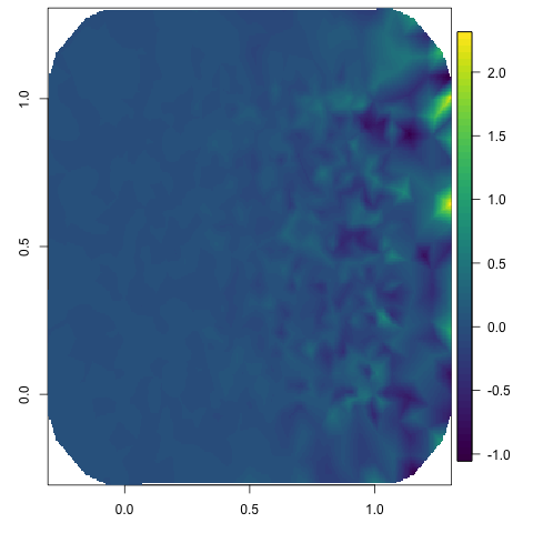
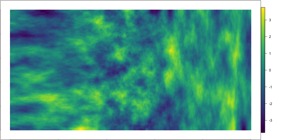
When modelling precipitation, we know that mountains influence the spatial distribution of the amount of precipitation. In particular, the amount of precipitation can be very different on either side of a mountain due to, for example, orographic effects. To build more realistic models for the covariance structure, we need to be able to allow both the mean structure and the covariance structure to vary in space. If covariates that can explain the variations are available, it is useful to allow the covariance structure to vary as a function of covariates, e.g. elevation. Lindgren et al., (2011) and Ingebrigtsen et al., (2014) include the covariates in the covariance structure by using the operator

$$\mathcal{L}_{2}=\left(\kappa(\boldsymbol{s})^{2}-\nabla\cdot\nabla\right)\tau(\boldsymbol{s}),$$

where the parameters vary in space as sums of known basis functions $b_{k}(\boldsymbol{s})$,

$$\log\tau(\boldsymbol{s})=\theta_{1}^{\tau}+\sum_{k=2}^{K}b_{k}(\boldsymbol{s})\theta_{k}^{\tau},$$

and similarly for $\kappa(\boldsymbol{s})$. See Figure 3 for an example of a simulation from a model with spatially varying marginal variance.

In practice, estimating both the mean structure and the covariance structure from a single realization of a spatial process may lead to inaccurate estimates and poorly identified parameters since the mean structure and the covariance structure are not separately identifiable. Ingebrigtsen et al., (2015) investigate estimation of models with covariates in both the mean structure and the covariance structure using multiple realizations. This model is implemented in R-INLA with the options B.tau and B.kappa in inla.spde2.matern.

Figure 3: Simulation from the model by Ingebrigtsen et al., (2014), as you decrease or increase $\tau$, increasing or decreasing the variance, from west to east.

6.2 The Barrier model

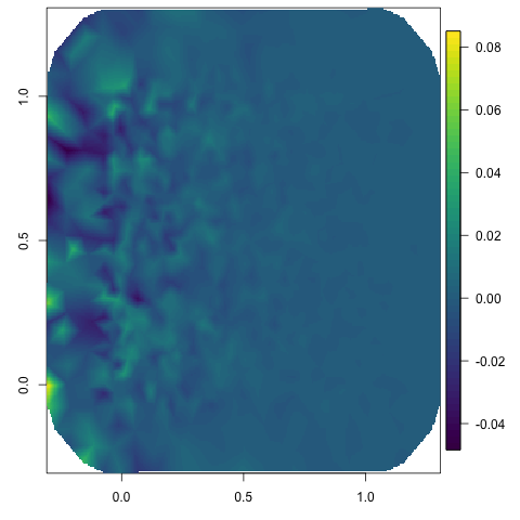
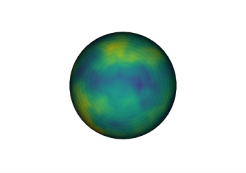
When modelling aquatic animals near a coastline, the stationary model smooths over islands and peninsulas, leading to unrealistic models. Further, stopping the mesh at the coastline imposes the Neumann boundary conditions, also leading to unrealistic models. Bakka et al., (2018) develop the Barrier model, defining the operator

$$\mathcal{L}_{3}=\sigma^{-1}\frac{2}{\pi r(\boldsymbol{s})^{2}}\left[1-\nabla\cdot\frac{r(\boldsymbol{s})^{2}}{8}\nabla\right],$$

with $r(\boldsymbol{s})\approx 0$ in a part of the study area, called the barrier area, and $r(\boldsymbol{s})=r$ in the rest of the study area. When modelling aquatic animals, the land area is a physical barrier to spatial correlation, see Figure 4 for an example simulation where the GRF smooths around the barrier. Other applications may include human activities on land, where water is a barrier, or they may represent roads, power lines, residential areas, or ship traffic, as physical barriers to a phenomenon. This model is implemented in R-INLA as inla.barrier.pcmatern, and, since the sparsity of the precision matrix is the same as for the corresponding stationary model, the computational cost is roughly the same.

Figure 4: Example correlation surface for the Barrier model by Bakka et al., (2018). The grey region acts as a physical barrier to spatial correlation, forcing the model to smooth around this barrier.

6.3 Spatially varying anisotropy

When modelling environmental data the assumption of isotropy may be questionable because directional effects such as wind may cause higher dependence in one direction than another. A simple way to achieve this in a stationary model is geometric anisotropy. Geometric anisotropy is equivalent to a linear transformation of the spatial coordinates and can be achieved by replacing the differential operator with

$$\mathcal{L}_{4}=\kappa^{2}-\nabla\cdot\text{\bf H}\nabla,$$

where H is a $2\times 2$ positive-definite matrix.

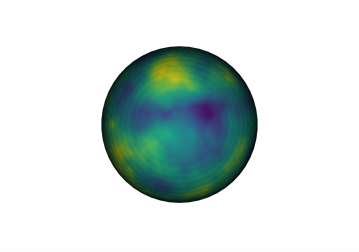
However, directional effects such as wind may vary over the spatial domain of interest and motivate non-stationarity in the anisotropy. Fuglstad et al., 2015a discuss how to make the anisotropy spatially varying by allowing H to vary spatially, and Fuglstad et al., 2015b discuss a generalisation where both $\kappa$ and H vary and show that this controls both spatially varying marginal standard deviations and spatially varying correlation structure. Figure 5 shows a simulation from a model where the anisotropy varies continuously from extra horizontal dependence on the left hand side to extra vertical dependence in the right hand side. This model was not implemented in R-INLA, when it was developed, but by using the new rgeneric framework (Rue et al.,, 2017) this is now possible. SPDE models with locally varying Laplacian can be interpreted as a change of metric in a differentiable manifold, which leads to a substantial overlap with the non-stationary models generated by the deformation method by Sampson and Guttorp, (1992).

Figure 5: Simulation of anisotropic field from the model by Fuglstad et al., 2015a . In the west part of the plot there is a strong horisontal dependence, while in the east part there is a strong vertical dependence.

6.4 SPDEs on manifolds

When modelling data on a global scale, using a rectangular subdomain of $\mathbb{R}^{2}$ is problematic because it is hard to avoid singularities near the poles and to construct covariance functions that make sense when transformed to the true spherical geometry. Covariance functions that are valid on $\mathbb{R}^{3}$ are valid on the sphere if chordal distances are used, and some families of covariance functions are valid when great circle distances are used, but validity of a covariance function using great circle distance does not follow from validity on $\mathbb{R}^{2}$ or $\mathbb{R}^{3}$ (Huang et al.,, 2011).

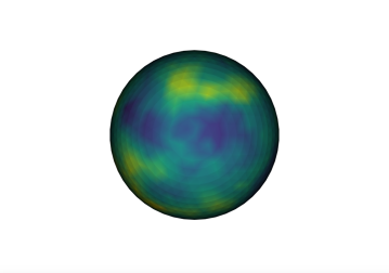
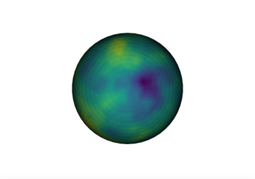
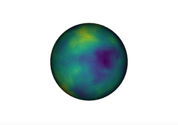
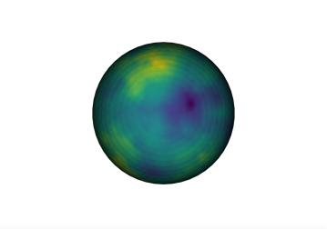
A major advantage of the SPDE approach is that if a two-dimensional mesh can be created for the domain of interest, then the resulting two-dimensional manifold structure can be used to interpret the operator $\mathcal{L}$ and the SPDE can be solved in the same way as for a triangulation of a subdomain of $\mathbb{R}^{2}$. In theory, meshes can be created for many kinds of two-dimensional manifold, but the important one for handling global data is the sphere $\mathbb{S}^{2}$. This is implemented as inla.mesh.create(globe=...) for a semi-regular discretisation of the entire globe, but the same subdomain techniques as on $\mathbb{R}^{2}$ can be used, after conversion of projected coordinates, to Euclidean 3-dimensional coordinates. This conversion can be automated by using the Coordinate Reference System (CRS) specification that usually accompany large scale spatial data, that specify which planar projection was used for the planar coordinates, such as UTM or longitude and latitude. By specifying what coordinate space the mesh should be built on, optionally with the aid of the inla.CRS function, and providing data as spatial objects with the sp package (Pebesma and Bivand,, 2005; Bivand et al., 2013b, ), conversion between projected and spherical coordinates is carried out behind the scenes. The implemented SPDE models do not use the CRS information to compensate for projection shape distortion, so the choice of space determines a degree of local anisotropy. For large-scale phenomena on the globe, building the analysis mesh as a subset of the Euclidean sphere is therefore often beneficial, as it more closely resembles reality. Any other manifold that is locally flat can in theory also be used, but currently requires the user to supply their own pre-generated mesh. It is also possible to generalise the operators and the SPDE approach to higher dimensions, as gradients and divergence have natural extension to 3 or more dimensions. In Figure 6 we show an example simulation of the model in Section 6.5 on the sphere, and refer to Zhang et al., (2016) for an application to three dimensional seismic inversion.

6.5 Non-separable space-time model

Separable space-time models are convenient, but not always appropriate; if we have a phenomenon that follows the heat equation, the resulting field is non-separable. There are an infinite number of ways non-separability can be described, but of special interest is a non-separable model that is closely linked to the heat equation, as this is one of the most common models in physics. Krainski, (2018) refers to the separable space-time model that is the Kronecker of Matérn and AR(1) as

$$\mathcal{L}_{5}=\left(\phi+\frac{\partial}{\partial t}\right)^{\alpha_{t}}(1-\gamma_{\mathcal{E}}\Delta)^{\alpha_{\mathcal{E}}/2},$$ (21)

and changes this to

$$\mathcal{L}_{6}=\left(\gamma_{t}\frac{\partial}{\partial t}-\Delta\right)^{\alpha_{t}}(1-\gamma_{\mathcal{E}}\Delta)^{\alpha_{\mathcal{E}}/2}$$ (22)

to produce a non-separable space-time model that is closely linked to the heat equation. Applications of this include temperature modelling on the globe, see Figure 6 for a simulated example. One key advantage when considering a discretisation approach based in Lindgren et al., (2011) is that the precision matrix for this model has sparsity similar to the one for the separable model, thus not adding computational burden. Krainski, (2018) consider some marginal properties of the resulting multivariate Gaussian disribution to understand the model parameters. Research is underway to understand for which applications this type of non-separability is more appropriate than a separable model. This and other related models are still development and we plan to implement them in R-INLA in the near future.

Figure 6: Simulation for the non-separable model by Krainski, (2018) on the sphere, for 6 time points (left to right, top to bottom).

6.6 General smoothness

The spatial operators we have discussed so far, $\mathcal{L}_{i}$, $i=1,\ldots,4$, are of second order. This explicitly determines the differentiability of the resulting random fields $u(\boldsymbol{s})$. To define models with different smoothness, the operator can be replaced by $\mathcal{L}_{i}^{\alpha/2}$, where $\alpha>0$ is a parameter determining the smoothness of the field. In this case, a restriction with the SPDE approach is that it is only computable if $\alpha$ is an integer, as in equation (11). This is typically not a major restriction, since $\alpha$ is difficult to estimate, but may be important in some cases (Stein,, 2012).

The parsimonious fractional approximation, which is implemented in R-INLA for the stationary Matérn model, is not applicable for the more general non-stationary models. However, Bolin and Kirchner, (2018) propose a rational SPDE method that is computable for any $\alpha>0$, and which has a higher accuracy than the parsimonious approximation for Matérn model. It combines the FEM approximation in space with a rational approximation of the function $x^{-\alpha/2}$ in order to compute an approximation of $u(\boldsymbol{s})$ on the form $\boldsymbol{u}=\text{\bf P}\text{\bf x}$, where $\boldsymbol{x}\sim\mathcal{N}(\text{\bf 0},\text{\bf Q}^{-1})$, and P and Q are sparse matrices. This approximation facilitates including $\alpha$ as a parameter that is estimated from the data, and fits in the INLA framework, but is not yet included in the package.

6.7 Non-Gaussian spatial fields

Figure 7: A simulation of a Matérn SPDE model driven by NIG noise.

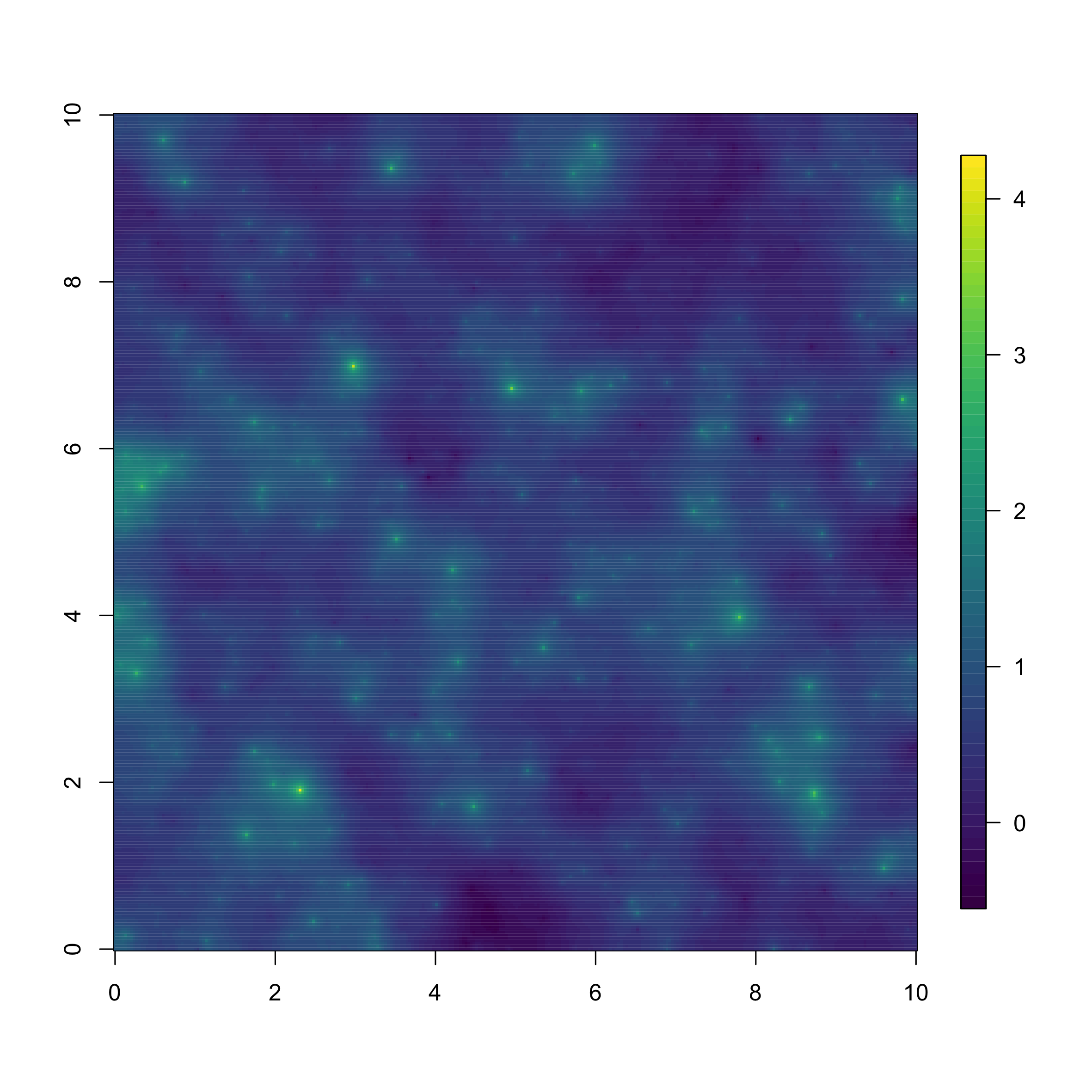
If the process of interest has features that cannot be captured by a Gaussian model, such as asymmetry in the sample paths or skewness in the marginal distributions, non-Gaussian Matérn-like fields can be defined by replacing the driving noise $\mathcal{W}$ by other non-Gaussian models. A simulation from a model like this can be seen in Figure 7. The model that is used for the simulation is

$$(\kappa^{2}-\Delta)(\tau u)=\mathcal{M},$$

where $\mathcal{M}$ is normal inverse Gaussian (NIG) noise, see Wallin and Bolin, (2015) for a formal definition. As in the Gaussian case, the process $u(\boldsymbol{s})$ has a Matérn covariance function, but the model has two additional parameters $\mu$ and $\gamma$ that respectively control skewness and tails of the marginal distributions. Using the parametrisation of the NIG noise from Bolin and Wallin, (2018), to assure that $u(\boldsymbol{s})$ has zero mean, and discretising the model using the FEM, yields the discretised model

$$\begin{split}\boldsymbol{u}|\tau,\kappa,\mu,\boldsymbol{v}&\sim\mathcal{N}(\tau^{-1}\mu\text{\bf K}^{-1}(\boldsymbol{v}-\boldsymbol{h}),\tau^{-2}\text{\bf K}^{-1}\operatorname{diag}(\boldsymbol{v})\text{\bf K}^{-T}),\\ \boldsymbol{v}|\gamma&\sim IG(\gamma^{2},\gamma^{2}\boldsymbol{h}^{2}).\end{split}$$ (23)

Here $\boldsymbol{v}$ is a vector of independent inverse Gaussian (IG) distributed variables and $h_{i}=\langle\phi_{i},1\rangle$.

Thus, the model is Gaussian conditionally on $\boldsymbol{v}$, where the parameter $\mu$ controls the mean of $\boldsymbol{u}|\boldsymbol{v}$. Comparing (23) with the corresponding Gaussian model (11), we note that the matrix C, with elements $C_{ii}=h_{i}$, has been replaced by a matrix with IG distributed elements satisfying $\mathbb{E}(v_{i})=h_{i}$. Because of this representation, it is easy to simulate non-Gaussian SPDE models using R-INLA. However, the INLA methodology cannot be used for inference in this case since the models are intrinsically non-Gaussian. Inference can instead be performed using stochastic gradient methods (Bolin and Wallin,, 2018).

6.8 Additional work

The models we have illustrated in this section are just scratching the surface of the possibilities for extending the simple Gaussian and isotropic covariance structures with the SPDE approach. Systems of SPDEs have been used to create multivariate spatial fields (Hu and Steinsland,, 2016; Hu et al., 2013b, ; Hu et al., 2013a, ; Bolin and Wallin,, 2018) and to generate more flexible anisotropic and oscillating covariance structures both on $\mathbb{R}^{d}$ and on the sphere (Bolin and Lindgren,, 2011; Barman and Bolin,, 2018). Yue et al., (2014) develops adaptive Bayesian splines based on the SPDE approach.

7 R-packages building on R-INLA

R-INLA is freely available from www.r-inla.org and open source, and there are multiple R-packages for discretely indexed spatial models defined on top of R-INLA. Their goal is to make the models more easily accessible for the applied researcher and/or offer additional functionality. Brown and Zhou, (2016); Brown, (2015) provide the package diseasemapping, which allows the user to implement Poisson regression models incorporating fixed effects and either the BYM or BYM2 model including PC priors. The R-package SUMMER (Martin and Li,, 2017) uses the classical BYM model for small area estimation of under-5 mortality based on survey data, see also Mercer et al., (2015). The results of different spatial models fitted with R-INLA to the same dataset can be combined through the R-package INLABMA (Bivand et al.,, 2015).

Very recently, the Shiny app SSTCDapp (http://www.unavarra.es/spatial-statistics-group/shiny-app) has been introduced, which allows the estimation of different discrete space and space-time models using R-INLA in a user-friendly way without R-code Ugarte et al., (2014); Goicoa et al., (2017); Adin et al., (2017). The app provides different descriptive statistics and supports several spatial and temporal model components. Furthermore, the four proposed space-time interaction types by Knorr-Held, (2000) are available, and the authors offer tutorials that explain the usage of the app.

Multiple packages for continuously indexed spatial models have also been developed on top of R-INLA. Brown, (2015) provides an easier interface to the SPDE models for geostatistical modelling in the package geostatsp, and Bolin and Lindgren, (2015) provides a package for calculating credible regions and excursion sets based on the output from R-INLA in the package excursions (Bolin and Lindgren,, 2018). The inlabru package (Bachl et al.,, 2018, https://inlabru.org/) provides a new general R-INLA user interface that in particular simplifies the specification of spatial and spatio-temporal models, by hiding all the inla.stack code from the user. It also extends the available class of models to mildly non-linear predictor models, and provides a predict function for non-linear posterior prediction based on i.i.d. posterior samples. Since it was initially developed for ecological survey data, it has special support for point process data. All these packages are available on CRAN.

8 Discussion

Reformulating spatial models into a form that is suitable for R-INLA can be challenging, but has great rewards. Within R-INLA, we can easily combine the spatial effect with other random effects, fixed effects or complex likelihoods to create complex spatial or spatio-temporal models. The INLA method allows fast Bayesian inference and makes full Bayesian inference possible for models that before were considered infeasible, or would require time-consuming and careful implementation of a sampler. Further, the speed-up for small models means that they can be run multiple times, e.g. for cross-validation. An important advantage for users is that adding model components, using non-Gaussian observation likelihoods or multiple likelihoods, and extending to separable space-time models, require little additional implementation effort.

The INLA methodology is centered around precision matrices, and CAR models like the Besag model, which by design have sparse precision matrices, are automatically well-suited for R-INLA. Continuously indexed models are more challenging, as they must be discretised in a form that admits a sparse CAR structure and parametrising CAR models directly is not a robust approach. However, the SPDE approach allows us to create a CAR structure for a continuously indexed discrete approximation of the spatial field by discretising an SPDE. This adds difficulty in understanding and setting up the problem, but we believe the comment made by Lindgren et al., (2011) is still valid:

…the approach comes with an implementation and preprocessing cost for setting up the models, as it involves the SPDE, triangulations and GMRF representations, but we firmly believe that such costs are unavoidable when efficient computations are required.

Purely applied users have little need to understand the FEM or SPDEs, beyond learning how to create a reasonable mesh and the connection between the spatial resolution and meshes. For statistical researchers, learning the SPDE approach requires a more significant effort and a more detailed study of the theory of Gaussian random fields, but it also produces generally straight-forward and stable results. Statistical models following the SPDE approach tend to work as intended, without many surprises and without the need to make clever—and often hidden—choices that are specialised for individual cases. The development of the advanced models in Section 6 was not easy, but the approach was straight-forward, in the sense that the research resulted in stable algorithms with behaviour “as intended”. The trade-off we have from using the SPDE approach in our research is that, instead of studying different tools for each generalisation of the model, we can study general tools used in numerics and physics and ways to discretise a differential operator, and apply this to the SPDE formulation.

The development of computationally tractable advanced models in space and space-time is not a simple task. We are fortunate to have many inquisitive and demanding users who challenge us to expand our research to fill the gaps that are necessary for good statistical problem solving. One of the hotly disputed topics is the question of what priors to use, including what interpretable parametrisations to define them on, and we consider the development of default priors, that we can stand behind, to be one of the biggest advances in R-INLA. There are other topics where there is still much work left to do, specifically for stability/robustness/sensitivity and for model comparison criteria.

Non-stationary models are often applied to space-time data, as replicates are needed to infer the non-stationarity, automatically putting them in competition with non-separable models. At this time, the focus is on implementing and documenting different non-stationary and non-separable models in R-INLA. The aim is to lay the groundwork for a future literature rich with examples and comparisons for a wide range of applications of these advanced models. After gaining the necessary practical experience with these methods, we can start answering the question of “when you should use what model”, e.g. in what applications is a separable space-time model with one specific type of non-stationary spatial structure the most relevant model.

The main computational challenge for the future is space-time models. At the time of this review, R-INLA can deal with applications with a hundred thousand dimensions in the space-time representation. However, having 100 nodes in each spatial and temporal direction gives a million dimensions, which is where R-INLA fails, and 100 nodes is a decent, but not very fine, resolution. Parallel computing may be able to overcome this obstacle, and we are currently investigating adequate approximations and factorisation methods that run well in parallel.

To sum up, for a particular application the question is almost never “what is the right thing to do”, but rather “what is the best thing to do that can be implemented and run in the limited time available”. The tools presented in this review have been successful in answering this question for many different applications, especially those that require more advanced models, and we continue to develop these tools to push the boundaries of applied statistical modelling.

9 Acknowledgements

The authors acknowledge comments from G. Konstantinoudis and from the referees.

Appendix A Appendix

A.1 Details on the BYM2 model

For the BYM2 model (see Section 3.2), we propose to use the penalised complexity (PC) framework developed by Simpson et al., (2017) to define priors for $\tau$ and $w$. This implies the use of an exponential prior with parameter $\lambda$ for the standard deviation $1/\sqrt{\tau}$. The parameter $\lambda$ can be elicited using the prior probability statement $\pi((1/\sqrt{\tau})>U)=\alpha$, which gives $\lambda=-\log(\alpha)/U$. Since $\tau$ represents the marginal precision, it can be directly related to the total residual relative risk, for which an intuitive interpretation is available. Simpson et al., (2017) give the rule of thumb that the marginal standard deviation of u with $\text{\bf Q}=\text{\bf I}$, after the exponential distribution for $1/\sqrt{\tau}$ is integrated out, is about $0.31U$ when $\alpha=0.01$. Believing for example that the residual relative risk lies with a probability of $0.99$ within the interval $(0.4,2.5)$, this would lead to an approximate interval $(-0.92,0.92)$ on the linear predictor scale assuming a log link. The marginal standard deviation of the spatial effect is assumed to be $0.92/2.58\approx 0.36$ which gives parameters $U=1.16$ and $\alpha=1\%$ in the PC prior for $\tau$.

The PC prior for the weight $w$, interpreted as the proportion of the variability contributed by the structured component, is not available in closed form (Simpson et al.,, 2017), but a probability contrast Prob($w<U)=\alpha$ can be used to specify its parameter. The use of PC priors allows the flexible, in some cases overfitting, model (7) to shrink sequentially towards two base models. The prior first shrinks towards a model without any spatial variation, i.e. setting $\tau$ to infinity, then shrinking towards a model with only unstructured variability, i.e. setting $w=0$. This desired behaviour has been shown by Riebler et al., (2016) and is not achievable by other commonly used priors. We note that Riebler et al., (2016) recommend the use of the BYM2 model over the Leroux model.

A.2 Details on the approximation of the Matérn field on a grid

Assume that the Gaussian random field $u$ is observed on an $M\times N$ grid, indexed by row $i$ and column $j$, where the distance between neighbouring observation locations are $h$ both vertically and horizontally. We can use central differences to construct a discrete representation of $\mathcal{L}_{1}$,

$$\text{\bf L}_{1} =\kappa^{2}\text{\bf I}+\text{\bf D}$$ (24)

$$D_{a,b} =\begin{cases}4/h^{2},&a=b,\\ -1/h^{2},&a\sim b,\\ 0,&\text{otherwise},\end{cases}$$ (25)

where I is an $MN\times MN$ identity matrix, $a=(i,j)\sim b=(i^{*},j^{*})$ if $a$ and $b$ are first-order neighbours, and periodic boundary conditions are used to avoid boundary corrections for D.

To visualise discrete operators, we use computational stencils,

1D∝h−2​ -14-1-1L1∝h−2​ -1κ2h2+4-1-1formulae-sequenceproportional-toIfragments 1missing-subexpressionmissing-subexpressionmissing-subexpressionformulae-sequenceproportional-toDsuperscriptℎ2fragments -14-1missing-subexpression-1missing-subexpressionproportional-tosubscriptL1superscriptℎ2fragments -1fragmentsκ2h24-1missing-subexpression-1missing-subexpression\text{\bf I}\propto\begin{tabular}[]{|c|c|c|}\hline\cr&&\\ \hline\cr&1&\\ \hline\cr&&\\ \hline\cr\end{tabular}\quad\text{\bf D}\propto h^{-2}\ \begin{tabular}[]{|c|c|c|}\hline\cr&- 1&\\ \hline\cr-1&4&-1\\ \hline\cr&-1&\\ \hline\cr\end{tabular}\quad\text{\bf L}_{1}\propto h^{-2}\ \begin{tabular}[]{|c|c|c|}\hline\cr&-1&\\ \hline\cr-1&$\kappa^{2}h^{2}+4$&-1\\ \hline\cr&-1&\\ \hline\cr\end{tabular}

- 1-1- 1-1

where the central value is the value on the diagonal of the matrix, the value above the centre is the matrix element for the entry representing a grid cell and its neighbour to the north, etc. The constant $h^{-2}$ outside of the computational stencil is a constant multiplying the entire matrix. Note that stencils are often rotationally symmetric, and they may use larger neighbourhoods.

Since the concept of discretised differential operator is of fundamental importance to the SPDE approach, we now present a detailed numerical example in $\mathbb{R}^{1}$.

Example A.1.

Let the differential operator be the second derivative,

$$\mathcal{L}_{1\text{D}}=\frac{\ \mathrm{d}}{\ \mathrm{d}x}\frac{\ \mathrm{d}}{\ \mathrm{d}x}.$$

If the operator is applied to the function $f(x)=5x^{2}+\sin(15x)$, a new function

$$g(x)=\mathcal{L}_{1D}(f)(x) =\frac{\ \mathrm{d}}{\ \mathrm{d}x}\frac{\ \mathrm{d}}{\ \mathrm{d}x}f(x)$$

$$=10-15^{2}\sin(15x),$$

is produced and the result is just the second-order derivative of $f$.

If $u$ is discretised to a grid where the distance between neighbouring grid cells is $h$, the operator $\mathcal{L}_{1\text{D}}$ can be discretised to a matrix $\text{\bf L}_{1\text{D}}$, with computational stencil

$$\text{\bf L}_{1\text{D}}\propto h^{-2}\ \begin{tabular}[]{|c|c|c|}\hline\cr 1&-2&1\\ \hline\cr\end{tabular}.$$

The stencil corresponds to the standard central difference approximation to the second-order derivative,

$$g(x) =\lim_{h\to 0}\frac{f^{\prime}(x+h/2)-f^{\prime}(x-h/2)}{h}$$

$$=\lim_{h\to 0}\frac{(f(x+h)-f(x))-(f(x)-f(x-h))}{h^{2}}$$

$$\approx h^{-2}(1f(x+h)-2f(x)+1f(x-h)).$$

The stencil gives a matrix with $-2h^{-2}$ on the diagonal, $1h^{-2}$ on the upper and lower diagonal, and 0 otherwise.

A small example is shown in Figure 8, where we have used an equally-spaced grid with $h=0.1$, and compare $f(x)$ to $\boldsymbol{f}$, and $\text{\bf L}_{1\text{D}}\boldsymbol{f}$ to the values of $\mathcal{L}_{1\text{D}}f$. The operator $\mathcal{L}_{1\text{D}}$ was used by Lindgren and Rue, (2008) to construct an approximation for the second-order random walk for irregular locations.

Figure 8: Example function $f$ (left plot) and $g=\mathcal{L}_{1\text{D}}f$ (right plot). The black pluses are the vector $\boldsymbol{f}$ representing the continuous function $f$ (black line), similarly with $\boldsymbol{g}$ and $g$. The blue circles is the discrete operator applied to the vector, i.e. $\text{\bf L}_{1\text{D}}\boldsymbol{f}$, which is close to the discretisation $\boldsymbol{g}$ of $g$.

References

- Adin et al., (2017) Adin, A., Martínez-Beneito, M., Botella-Rocamora, P., Goicoa, T., and Ugarte, M. (2017). Smoothing and high risk areas detection in space-time disease mapping: a comparison of P-splines, autoregressive, and moving average models. Stochastic Environmental Research and Risk Assessment, 31(2):403–415.
- Bachl et al., (2018) Bachl, F. E., Lindgren, F., Borchers, D. L., Simpson, D., and Scott-Hayward, L. (2018). inlabru: Spatial Inference using Integrated Nested Laplace Approximation. R package version 2.1.3.
- Baddeley et al., (2015) Baddeley, A., Rubak, E., and Turner, R. (2015). Spatial point patterns: methodology and applications with R. CRC Press.
- Bakka, (2018) Bakka, H. (2018). How to solve the stochastic partial differential equation that gives a Matérn random field using the finite element method. arXiv preprint arXiv:1803.03765.
- Bakka et al., (2018) Bakka, H., Vanhatalo, J., Illian, J., Simpson, D., and Rue, H. (2018). Non-stationary Gaussian models with physical barriers. arXiv preprint arXiv:1608.03787.
- Barber et al., (2016) Barber, X., Conesa, D., Lladosa, S., and López-Quílez, A. (2016). Modelling the presence of disease under spatial misalignment using Bayesian latent Gaussian models. Geospatial health, 11(1).
- Barman and Bolin, (2018) Barman, S. and Bolin, D. (2018). A three-dimensional statistical model for imaged microstructures of porous polymer films. Journal of Microscopy, 269(3):247–258.
- Barthelmé et al., (2013) Barthelmé, S., Trukenbrod, H., Engbert, R., and Wichmann, F. (2013). Modeling fixation locations using spatial point processes. Journal of vision, 13(12):1–1.
- Beguin et al., (2017) Beguin, J., Fuglstad, G.-A., Mansuy, N., and Paré, D. (2017). Predicting soil properties in the Canadian boreal forest with limited data: Comparison of spatial and non-spatial statistical approaches. Geoderma, 306:195–205.
- Bernardinelli et al., (1995) Bernardinelli, L., Clayton, D., and Montomoli, C. (1995). Bayesian estimates of disease maps: How important are priors? Statistics in Medicine, 14(21-22):2411–2431.
- Besag, (1974) Besag, J. (1974). Spatial interaction and the statistical analysis of lattice systems (with discussion). Journal of the Royal Statistical Society, Series B, 36(2):192–225.
- Besag et al., (1991) Besag, J., York, J., and Mollié, A. (1991). Bayesian image restoration, with two applications in spatial statistics. Annals of the institute of statistical mathematics, 43(1):1–20.
- Bhatt et al., (2015) Bhatt, S., Weiss, D. J., Cameron, E., Bisanzio, D., Mappin, B., Dalrymple, U., Battle, K. E., Moyes, C. L., Henry, A., Eckhoff, P. A., Wenger, E. A., Briët, O., Penny, M. A., Smith, T. A., Bennett, A., Yukich, J., Eisele, T. P., Griffin, J. T., Fergus, C. A., Lynch, M., Lindgren, F., Cohen, J. M., Murray, C. L. J., Smith, D. L., Hay, S. I., Cibulskis, R. E., and Gething, P. W. (2015). The effect of malaria control on plasmodium falciparum in Africa between 2000 and 2015. Nature, (526):207–211.
- (14) Bivand, R., Hauke, J., and Kossowski, T. (2013a). Computing the Jacobian in Gaussian spatial autoregressive models: an illustrated comparison of available methods. Geographical Analysis, 45(2):150–179.
- Bivand and Lewin-Koh, (2017) Bivand, R. and Lewin-Koh, N. (2017). maptools: Tools for Reading and Handling Spatial Objects. R package version 0.9-2.
- Bivand and Piras, (2015) Bivand, R. and Piras, G. (2015). Comparing implementations of estimation methods for spatial econometrics. Journal of Statistical Software, Articles, 63(18).
- Bivand et al., (2014) Bivand, R. S., Gómez-Rubio, V., and Rue, H. (2014). Approximate Bayesian inference for spatial econometrics models. Spatial Statistics, 9:146–165.
- Bivand et al., (2015) Bivand, R. S., Gómez-Rubio, V., and Rue, H. (2015). Spatial data analysis with R-INLA with some extensions. Journal of Statistical Software, 63(20):1–31.
- (19) Bivand, R. S., Pebesma, E., and Gomez-Rubio, V. (2013b). Applied spatial data analysis with R, Second edition. Springer, NY.
- Blangiardo and Cameletti, (2015) Blangiardo, M. and Cameletti, M. (2015). Spatial and Spatio-temporal Bayesian Models with R-INLA. John Wiley & Sons.
- Blangiardo et al., (2013) Blangiardo, M., Cameletti, M., Baio, G., and Rue, H. (2013). Spatial and spatio-temporal models with R-INLA. Spatial and Spatio-Temporal Epidemiology, 3(December):39–55.
- Bolin and Kirchner, (2018) Bolin, D. and Kirchner, K. (2018). The rational SPDE approach for Gaussian random fields with general smoothness. arXiv preprint arXiv:1711.04333.
- Bolin and Lindgren, (2011) Bolin, D. and Lindgren, F. (2011). Spatial models generated by nested stochastic partial differential equations, with an application to global ozone mapping. Annals of Applied Statistics, 5(1):523–550.
- Bolin and Lindgren, (2015) Bolin, D. and Lindgren, F. (2015). Excursion and contour uncertainty regions for latent Gaussian models. Journal of the Royal Statistical Society: Series B (Statistical Methodology), 77(1):85–106.
- Bolin and Lindgren, (2017) Bolin, D. and Lindgren, F. (2017). Quantifying the uncertainty of contour maps. Journal of Computational and Graphical Statistics, 26(3):513–524.
- Bolin and Lindgren, (2018) Bolin, D. and Lindgren, F. (2018). Calculating probabilistic excursion sets and related quantities using excursions. Journal of Statistical Software, page in press.
- Bolin and Wallin, (2018) Bolin, D. and Wallin, J. (2018). Multivariate Type-G Matérn fields. arXiv preprint arXiv:1606.08298.
- Bosco et al., (2017) Bosco, C., Alegana, V., Bird, T., Pezzulo, C., Bengtsson, L., Sorichetta, A., Steele, J., Hornby, G., Ruktanonchai, C., Ruktanonchai, N., et al. (2017). Exploring the high-resolution mapping of gender-disaggregated development indicators. Journal of The Royal Society Interface, 14(129):20160825.
- Boudreau et al., (2017) Boudreau, S. A., Shackell, N. L., Carson, S., and den Heyer, C. E. (2017). Connectivity, persistence, and loss of high abundance areas of a recovering marine fish population in the northwest atlantic ocean. Ecology and evolution, 7(22):9739–9749.
- Brenner and Scott, (2007) Brenner, S. and Scott, R. (2007). The mathematical theory of finite element methods, volume 15. Springer Science & Business Media.
- Brown, (2015) Brown, P. E. (2015). Model-based geostatistics the easy way. Journal of Statistical Software, 63(12):1–24.
- Brown and Zhou, (2016) Brown, P. E. and Zhou, L. (2016). diseasemapping: Modelling Spatial Variation in Disease Risk for Areal Data. R package version 1.4.2.
- Cameletti et al., (2011) Cameletti, M., Ignaccolo, R., and Bande, S. (2011). Comparing spatio-temporal models for particulate matter in Piemonte. Environmetrics, 22(8):985–996.
- Carson et al., (2017) Carson, S., Shackell, N., and Flemming, J. M. (2017). Local overfishing may be avoided by examining parameters of a spatio-temporal model. PloS one, 12(9):e0184427.
- Dalrymple et al., (2017) Dalrymple, U., Cameron, E., Bhatt, S., Weiss, D. J., Gupta, S., and Gething, P. W. (2017). Quantifying the contribution of plasmodium falciparum malaria to febrile illness amongst African children. eLife, 6.
- Dean et al., (2001) Dean, C., Ugarte, M., and Militino, A. (2001). Detecting interaction between random region and fixed age effects in disease mapping. Biometrics, 57(1):197–202.
- Diggle, (2003) Diggle, P. J. (2003). Statistical Analysis of Spatial Point Patterns, 2nd ed. Hodder Arnold, London.
- Dyer et al., (2017) Dyer, E. E., Cassey, P., Redding, D. W., Collen, B., Franks, V., Gaston, K. J., Jones, K. E., Kark, S., Orme, C. D. L., and Blackburn, T. M. (2017). The global distribution and drivers of alien bird species richness. PLoS biology, 15(1):e2000942.
- Etxeberria et al., (2017) Etxeberria, J., Goicoa, T., López-Abente, G., Riebler, A., and Ugarte, M. D. (2017). Spatial gender-age-period-cohort analysis of pancreatic cancer mortality in Spain (1990–2013). PloS one, 12(2):e0169751.
- Fonseca et al., (2017) Fonseca, V. P., Pennino, M. G., de Nóbrega, M. F., Oliveira, J. E. L., and de Figueiredo Mendes, L. (2017). Identifying fish diversity hot-spots in data-poor situations. Marine environmental research, 129:365–373.
- Freni-Sterrantino et al., (2018) Freni-Sterrantino, A., Ventrucci, M., and Rue, H. (2018). A note on intrinsic conditional autoregressive models for disconnected graphs. Spatial and Spatio-temporal Epidemiology, xx(xx):xx–xx. (to appear).
- Fuglstad and Beguin, (2018) Fuglstad, G.-A. and Beguin, J. (2018). Environmental mapping using Bayesian spatial modelling (INLA/SPDE): A reply to Huang et al.(2017). Science of The Total Environment, 624:596–598.
- (43) Fuglstad, G.-A., Lindgren, F., Simpson, D., and Rue, H. (2015a). Exploring a new class of non-stationary spatial Gaussian random fields with varying local anisotropy. Statistica Sinica, pages 115–133.
- (44) Fuglstad, G.-A., Simpson, D., Lindgren, F., and Rue, H. (2015b). Does non-stationary spatial data always require non-stationary random fields? Spatial Statistics, 14:505–531.
- Fuglstad et al., (2017) Fuglstad, G. A., Simpson, D., Lindgren, F., and Rue, H. (2017). Constructing priors that penalize the complexity of Gaussian random fields. Journal of the American Statistical Association, xx(xx):xx–xx. (to appear).
- Gakidou et al., (2017) Gakidou, E., Afshin, A., Abajobir, A. A., Abate, K. H., Abbafati, C., Abbas, K. M., Abd-Allah, F., Abdulle, A. M., Abera, S. F., Aboyans, V., et al. (2017). Global, regional, and national comparative risk assessment of 84 behavioural, environmental and occupational, and metabolic risks or clusters of risks, 1990-2016: a systematic analysis for the global burden of disease study 2016. Lancet, 390(10100):1345–1422.
- Goicoa et al., (2017) Goicoa, T., Adin, A., Ugarte, M., and Hodges, J. (2017). In spatio-temporal disease mapping models, identifiability constraints affect PQL and INLA results. Stochastic Environmental Research and Risk Assessment, pages 1–22.
- Golding et al., (2017) Golding, N., Burstein, R., Longbottom, J., Browne, A. J., Fullman, N., Osgood-Zimmerman, A., Earl, L., Bhatt, S., Cameron, E., Casey, D. C., et al. (2017). Mapping under-5 and neonatal mortality in Africa, 2000–15: a baseline analysis for the sustainable development goals. The Lancet, 390(10108):2171–2182.
- Gómez-Rubio et al., (2015) Gómez-Rubio, V., Bivand, R., and Rue, H. (2015). A new latent class to fit spatial econometrics models with integrated nested Laplace approximations. Procedia Envionmental Sciences, 27:116–118.
- Gómez-Rubio et al., (2014) Gómez-Rubio, V., Bivand, R. S., and Rue, H. (2014). Spatial models using Laplace approximation methods. In Fischer, M. and Nijkamp, P., editors, Handbook of Regional Science, pages 1401–1417. Springer Verlag, Berlin, Heidelberg.
- Gortázar et al., (2017) Gortázar, C., Fernández-Calle, L., Collazos-Martínez, J., Mínguez-González, O., and Acevedo, P. (2017). Animal tuberculosis maintenance at low abundance of suitable wildlife reservoir hosts: A case study in northern Spain. Preventive veterinary medicine, 146:150–157.
- Haas et al., (2011) Haas, S. E., Hooten, M. B., Rizzo, D. M., and Meentemeyer, R. K. (2011). Forest species diversity reduces disease risk in a generalist plant pathogen invasion. Ecology letters, 14(11):1108–1116.
- Heaton et al., (2017) Heaton, M. J., Datta, A., Finley, A., Furrer, R., Guhaniyogi, R., Gerber, F., Gramacy, R. B., Hammerling, D., Katzfuss, M., Lindgren, F., et al. (2017). Methods for analyzing large spatial data: A review and comparison. arXiv preprint arXiv:1710.05013.
- (54) Hu, X., Lindgren, F., Simpson, D., and Rue, H. (2013a). Multivariate Gaussian random fields with oscillating covariance functions using systems of stochastic partial differential equations. arXiv preprint arXiv:1307.1384.
- Hu and Steinsland, (2016) Hu, X. and Steinsland, I. (2016). Spatial modeling with system of stochastic partial differential equations. Wiley Interdisciplinary Reviews: Computational Statistics, 8(2):112–125.
- (56) Hu, X., Steinsland, I., Simpson, D., Martino, S., and Rue, H. (2013b). Spatial modelling of temperature and humidity using systems of stochastic partial differential equations. arXiv preprint arXiv:1307.1402.
- Huang et al., (2011) Huang, C., Zhang, H., and Robeson, S. M. (2011). On the validity of commonly used covariance and variogram functions on the sphere. Mathematical Geosciences, 43(6):721–733.
- Huang et al., (2017) Huang, J., Malone, B. P., Minasny, B., McBratney, A. B., and Triantafilis, J. (2017). Evaluating a Bayesian modelling approach (INLA-SPDE) for environmental mapping. Science of the Total Environment, 609:621–632.
- Humphreys et al., (2017) Humphreys, J. M., Elsner, J. B., Jagger, T. H., and Pau, S. (2017). A Bayesian geostatistical approach to modeling global distributions of lygodium microphyllum under projected climate warming. Ecological Modelling, 363:192–206.
- Illian et al., (2008) Illian, J. B., Penttinen, A., Stoyan, H., and Stoyan, D. (2008). Statistical analysis and modelling of spatial point patterns, volume 70. John Wiley & Sons.
- (61) Illian, J. B., Sørbye, S. H., and Rue, H. (2012a). A toolbox for fitting complex spatial point process models using integrated nested laplace approximation (inla). The Annals of Applied Statistics, pages 1499–1530.
- (62) Illian, J. B., Sørbye, S. H., Rue, H., and Hendrichsen, D. K. (2012b). Using INLA to fit a complex point process model with temporally varying effects – a case study. Journal of Environmental Statistics, 3(7).
- Ingebrigtsen et al., (2014) Ingebrigtsen, R., Lindgren, F., and Steinsland, I. (2014). Spatial models with explanatory variables in the dependence structure. Spatial Statistics, 8:20–38.
- Ingebrigtsen et al., (2015) Ingebrigtsen, R., Lindgren, F., Steinsland, I., and Martino, S. (2015). Estimation of a non-stationary model for annual precipitation in southern Norway using replicates of the spatial field. Spatial Statistics, 14:338–364.
- Innocent et al., (2017) Innocent, G. T., Gilbert, L., Jones, E. O., McLeod, J. E., Gunn, G., McKendrick, I. J., and Albon, S. D. (2017). Combining slaughterhouse surveillance data with cattle tracing scheme and environmental data to quantify environmental risk factors for liver fluke in cattle. Frontiers in veterinary science, 4.
- Jousimo et al., (2014) Jousimo, J., Tack, A. J. M., Ovaskainen, O., Mononen, T., Susi, H., Tollenaere, C., and Laine, A.-L. (2014). Ecological and evolutionary effects of fragmentation on infectious disease dynamics. Science, 344(6189):1289–1293.
- Knorr-Held, (2000) Knorr-Held, L. (2000). Bayesian modelling of inseparable space-time variation in disease risk. Statistics in Medicine, 19(17-18):2555–2567.
- Krainski, (2018) Krainski, E. T. (2018). Statistical Analysis of Space-time Data: New Models and Applications. PhD thesis, Norwegian University of Science and Technology.
- Krainski et al., (2017) Krainski, E. T., Lindgren, F., Simpson, D., and Rue, H. (2017). The r-inla tutorial on spde models. www.math.ntnu.no/inla/r-inla.org/tutorials/spde/spde-tutorial.pdf.
- Laurini, (2017) Laurini, M. P. (2017). The spatio-temporal dynamics of ethanol/gasoline price ratio in Brazil. Renewable and Sustainable Energy Reviews, 70:1–12.
- Lee et al., (2017) Lee, E. C., Arab, A., Goldlust, S., Viboud, C., and Bansal, S. (2017). Socio-environmental and measurement factors drive spatial variation in influenza-like illness. bioRxiv, page 112680.
- Lenzi et al., (2017) Lenzi, A., Pinson, P., Clemmensen, L. H., and Guillot, G. (2017). Spatial models for probabilistic prediction of wind power with application to annual-average and high temporal resolution data. Stochastic Environmental Research and Risk Assessment, 31(7):1615–1631.
- Leroux et al., (2000) Leroux, B. G., Lei, X., and Breslow, N. (2000). Estimation of disease rates in small areas: A new mixed model for spatial dependence. In Statistical Models in Epidemiology, the Environment, and Clinical Trials, pages 179–191. Springer.
- Lindgren and Rue, (2008) Lindgren, F. and Rue, H. (2008). A note on the second order random walk model for irregular locations. Scandinavian Journal of Statistics, 35(4):691–700.
- Lindgren and Rue, (2015) Lindgren, F. and Rue, H. (2015). Bayesian spatial modelling with R-INLA. Journal of Statistical Software, 63(19).
- Lindgren et al., (2011) Lindgren, F., Rue, H., and Lindström, J. (2011). An explicit link between Gaussian fields and Gaussian Markov random fields: the stochastic partial differential equation approach. Journal of the Royal Statistical Society: Series B (Statistical Methodology), 73(4):423–498.
- Lombardo et al., (2018) Lombardo, L., Opitz, T., and Huser, R. (2018). Point process-based modeling of multiple debris flow landslides using inla: an application to the 2009 messina disaster. Stochastic Environmental Research and Risk Assessment.
- López-Abente et al., (2017) López-Abente, G., Locutura-Rupérez, J., Fernández-Navarro, P., Martín-Méndez, I., Bel-Lan, A., and Núñez, O. (2017). Compositional analysis of topsoil metals and its associations with cancer mortality using spatial misaligned data. Environmental Geochemistry and Health, pages 1–12.
- Martin and Li, (2017) Martin, B. D. and Li, Z. R. (2017). SUMMER: Spatio-Temporal Under-Five Mortality Methods for Estimation. R package version 0.1.0.
- Martino et al., (2011) Martino, S., Akerkar, R., and Rue, H. (2011). Approximate Bayesian inference for survival models. Scandinavian Journal of Statistics, 38(3):514–528.
- Mathew et al., (2016) Mathew, B., Holand, A. M., Koistinen, P., Léon, J., and Sillanpää, M. J. (2016). Reparametrization-based estimation of genetic parameters in multi-trait animal model using integrated nested Laplace approximation. Theoretical and Applied Genetics, 129(2):215–225.
- Mejia et al., (2017) Mejia, A., Yue, Y. R., Bolin, D., Lindren, F., and Lindquist, M. A. (2017). A Bayesian general linear modeling approach to cortical surface fMRI data analysis. arXiv preprint arXiv:1706.00959.
- Mellor et al., (2018) Mellor, K. C., Meyer, A., Elkholly, D. A., Fournié, G., Long, P. T., Inui, K., Padungtod, P., Gilbert, M., Newman, S. H., Vergne, T., et al. (2018). Comparative epidemiology of highly pathogenic avian influenza virus h5n1 and h5n6 in vietnamese live bird markets: Spatiotemporal patterns of distribution and risk factors. Frontiers in Veterinary Science, 5:51.
- Mercer et al., (2017) Mercer, L. D., Safdar, R. M., Ahmed, J., Mahamud, A., Khan, M. M., Gerber, S., O’Leary, A., Ryan, M., Salet, F., Kroiss, S. J., et al. (2017). Spatial model for risk prediction and sub-national prioritization to aid poliovirus eradication in Pakistan. BMC medicine, 15(1):180.
- Mercer et al., (2015) Mercer, L. D., Wakefield, J., Pantazis, A., Lutambi, A. M., Masanja, H., and Clark, S. (2015). Space-time smoothing of complex survey data: small area estimation for child mortality. The annals of applied statistics, 9(4):1889.
- Møller et al., (1998) Møller, J., Syversveen, A. R., and Waagepetersen, R. P. (1998). Log Gaussian Cox processes. Scandinavian Journal of Statistics, 25:451–482.
- Moraga et al., (2017) Moraga, P., Cramb, S. M., Mengersen, K. L., and Pagano, M. (2017). A geostatistical model for combined analysis of point-level and area-level data using INLA and SPDE. Spatial Statistics, 21:27–41.
- Morosinotto et al., (2017) Morosinotto, C., Villers, A., Thomson, R. L., Varjonen, R., and Korpimäki, E. (2017). Competitors and predators alter settlement patterns and reproductive success of an intraguild prey. Ecological Monographs, 87(1):4–20.
- Musenge et al., (2013) Musenge, E., Chirwa, T. F., Kahn, K., and Vounatsou, P. (2013). Bayesian analysis of zero inflated spatiotemporal HIV/TB child mortality data through the INLA and SPDE approaches: applied to data observed between 1992 and 2010 in rural north east south Africa. International journal of applied earth observation and geoinformation, 22:86–98.
- Naeeim and Rahman, (2017) Naeeim, N. S. A. and Rahman, N. A. (2017). Estimating relative risk for dengue disease in peninsular Malaysia using INLA. Malaysian Journal of Fundamental and Applied Sciences, 13(4).
- Noor et al., (2014) Noor, A. M., Kinyoki, D. K., Mundia, C. W., Kabaria, C. W., Mutua, J. W., Alegana, V. A., Fall, I. S., and Snow, R. W. (2014). The changing risk of Plasmodium falciparum malaria infection in Africa: 2000-10: a spatial and temporal analysis of transmission intensity. The Lancet, 383(9930):1739–1747.
- Ntirampeba et al., (2017) Ntirampeba, D., Neema, I., and Kazembe, L. (2017). Joint spatial modelling of disease risk using multiple sources: an application on HIV prevalence from antenatal sentinel and demographic and health surveys in Namibia. Global health research and policy, 2(1):22.
- Opitz et al., (2018) Opitz, T., Huser, R., Bakka, H., and Rue, H. (2018). INLA goes extreme: Bayesian tail regression for the estimation of high spatio-temporal quantiles. Extremes (arxiv:802.01085), xx(xx):xx–. (to appear).
- Papoila et al., (2014) Papoila, A. L., Riebler, A., Amaral-Turkman, A., São-João, R., Ribeiro, C., Geraldes, C., and Miranda, A. (2014). Stomach cancer incidence in Southern Portugal 1998–2006: A spatio-temporal analysis. Biometrical Journal, 56(3):403–415.
- Paradinas et al., (2017) Paradinas, I., Conesa, D., López-Quílez, A., and Bellido, J. M. (2017). Spatio-temporal model structures with shared components for semi-continuous species distribution modelling. Spatial Statistics, 22:434–450.
- Pebesma and Bivand, (2005) Pebesma, E. J. and Bivand, R. S. (2005). Classes and methods for spatial data in R. R News, 5(2):9–13.
- Pereira et al., (2017) Pereira, S., Turkman, K. F., Correia, L., and Rue, H. (2017). Unemployment estimation: Spatial point referenced methods and models. arXiv preprint arXiv:1706.08320.
- Poggio et al., (2016) Poggio, L., Gimona, A., Spezia, L., and Brewer, M. J. (2016). Bayesian spatial modelling of soil properties and their uncertainty: The example of soil organic matter in scotland using r-inla. Geoderma, 277:69–82.
- Quiroz et al., (2015) Quiroz, Z. C., Prates, M. O., and Rue, H. (2015). A Bayesian approach to estimate the biomass of anchovies off the coast of Perú. Biometrics, 71(1):208–217.
- Renner et al., (2015) Renner, I. W., Elith, J., Baddeley, A., Fithian, W., Hastie, T., Phillips, S. J., Popovic, G., and Warton, D. I. (2015). Point process models for presence-only analysis. Methods in Ecology and Evolution, 6(4):366–379.
- Riebler et al., (2012) Riebler, A., Held, L., and Rue, H. (2012). Estimation and extrapolation of time trends in registry data—borrowing strength from related populations. The Annals of Applied Statistics, pages 304–333.
- Riebler et al., (2016) Riebler, A., Sørbye, S. H., Simpson, D., and Rue, H. (2016). An intuitive Bayesian spatial model for disease mapping that accounts for scaling. Statistical Methods in Medical Research, 25(4):1145–1165.
- Roopsind et al., (2017) Roopsind, A., Caughlin, T. T., Sambhu, H., Fragoso, J., and Putz, F. E. (2017). Logging and indigenous hunting impacts on persistence of large neotropical animals. Biotropica, 49(4):565–575.
- Rue and Held, (2005) Rue, H. and Held, L. (2005). Gaussian Markov Random Fields: Theory and Applications, volume 104 of Monographs on Statistics and Applied Probability. Chapman & Hall, London.
- Rue et al., (2009) Rue, H., Martino, S., and Chopin, N. (2009). Approximate Bayesian inference for latent Gaussian models using integrated nested Laplace approximations (with discussion). Journal of the Royal Statistical Society, Series B, 71(2):319–392.
- Rue et al., (2017) Rue, H., Riebler, A., Sørbye, S. H., Illian, J. B., Simpson, D. P., and Lindgren, F. K. (2017). Bayesian computing with INLA: A review. Annual Reviews of Statistics and Its Applications, 4(March):395–421.
- Rue and Tjelmeland, (2002) Rue, H. and Tjelmeland, H. (2002). Fitting Gaussian Markov random fields to Gaussian fields. Scandinavian Journal of Statistics, 29(1):31–50.
- Rutten et al., (2017) Rutten, L. J. F., Wilson, P. M., Jacobson, D. J., Agunwamba, A. A., Breitkopf, C. R., Jacobson, R. M., and Sauver, J. L. S. (2017). A population-based study of sociodemographic and geographic variation in HPV vaccination.
- Sadykova et al., (2017) Sadykova, D., Scott, B. E., De Dominicis, M., Wakelin, S. L., Sadykov, A., and Wolf, J. (2017). Bayesian joint models with inla exploring marine mobile predator–prey and competitor species habitat overlap. Ecology and Evolution.
- Sampson and Guttorp, (1992) Sampson, P. D. and Guttorp, P. (1992). Nonparametric estimation of nonstationary spatial covariance structure. Journal of the American Statistical Association, 87(417):108–119.
- (111) Schrödle, B. and Held, L. (2011a). A primer on disease mapping and ecological regression using INLA. Computational statistics, 26(2):241–258.
- (112) Schrödle, B. and Held, L. (2011b). Spatio-temporal disease mapping using INLA. Environmetrics, 22(6):725–734.
- Schrödle et al., (2012) Schrödle, B., Held, L., and Rue, H. (2012). Assessing the impact of a movement network on the spatiotemporal spread of infectious diseases. Biometrics, 68(3):736–744.
- Shaddick et al., (2018) Shaddick, G., Thomas, M. L., Green, A., Brauer, M., Donkelaar, A., Burnett, R., Chang, H. H., Cohen, A., Dingenen, R. V., Dora, C., et al. (2018). Data integration model for air quality: a hierarchical approach to the global estimation of exposures to ambient air pollution. Journal of the Royal Statistical Society: Series C (Applied Statistics), 67(1):231–253.
- Simpson et al., (2016) Simpson, D., Illian, J. B., Lindgren, F., Sørbye, S. H., and Rue, H. (2016). Going off grid: Computationally efficient inference for log-gaussian cox processes. Biometrika, 103(1):49–70.
- Simpson et al., (2017) Simpson, D. P., Rue, H., Riebler, A., Martins, T. G., and Sørbye, S. H. (2017). Penalising model component complexity: A principled, practical approach to constructing priors (with discussion). Statistical Science, 32(1):1–28.
- Sørbye and Rue, (2014) Sørbye, S. H. and Rue, H. (2014). Scaling intrinsic Gaussian Markov random field priors in spatial modelling. Spatial Statistics, 8(3):39–51.
- Stein, (2012) Stein, M. L. (2012). Interpolation of spatial data: some theory for kriging. Springer Science & Business Media.
- Thorson et al., (2017) Thorson, J. T., Ianelli, J. N., and Kotwicki, S. (2017). The relative influence of temperature and size-structure on fish distribution shifts: A case-study on walleye pollock in the bering sea. Fish and Fisheries.
- Ugarte et al., (2014) Ugarte, M. D., Adin, A., Goicoa, T., and Militino, A. F. (2014). On fitting spatio-temporal disease mapping models using approximate Bayesian inference. Statistical methods in medical research, 23(6):507–530.
- van Lieshout, (2000) van Lieshout, M. (2000). Markov point processes and their applications. Imperial College Press, London.
- Wakefield, (2007) Wakefield, J. (2007). Disease mapping and spatial regression with count data. Biostatistics, 8(2):158–183.
- Wakefield et al., (2018) Wakefield, J., Fuglstad, G.-A., Riebler, A., Godwin, J., Wilson, K., and Clark, S. J. (2018). Estimating under five mortality in space and time in a developing world context. Statistical Methods in Medical Research. In press.
- Wallin and Bolin, (2015) Wallin, J. and Bolin, D. (2015). Geostatistical modelling using non-Gaussian Matérn fields. Scandinavian Journal of Statistics, 42:872–890.
- Whittle, (1954) Whittle, P. (1954). On stationary processes in the plane. Biometrika, pages 434–449.
- Whittle, (1963) Whittle, P. (1963). Stochastic processes in several dimensions. Bull. Inst. Internat. Statist., 40:974–994.
- World Health Organization, (2016) World Health Organization (2016). Ambient air pollution: A global assessment of exposure and burden of disease.
- Yuan et al., (2017) Yuan, Y., Bachl, F. E., Lindgren, F., Borchers, D. L., Illian, J. B., Buckland, S. T., Rue, H., Gerrodette, T., et al. (2017). Point process models for spatio-temporal distance sampling data from a large-scale survey of blue whales. The Annals of Applied Statistics, 11(4):2270–2297.
- Yue et al., (2014) Yue, Y. R., Simpson, D., Lindgren, F., Rue, H., et al. (2014). Bayesian adaptive smoothing splines using stochastic differential equations. Bayesian Analysis, 9(2):397–424.
- Zhang, (2004) Zhang, H. (2004). Inconsistent estimation and asymptotically equal interpolations in model-based geostatistics. Journal of the American Statistical Association, 99(465):250–261.
- Zhang et al., (2016) Zhang, R., Czado, C., and Sigloch, K. (2016). Bayesian spatial modelling for high dimensional seismic inverse problems. Journal of the Royal Statistical Society: Series C (Applied Statistics), 65(2):187–213.