Minimum length RNA folding trajectories

Abstract

Background: Existent programs for RNA folding kinetics, such as Kinefold, Kinfold and KFOLD, implement the Gillespie algorithm to generate stochastic folding trajectories from an initial structure $s$ to a target structure $t$, in which each intermediate secondary structure is obtained from its predecessor by the application of a move from a given move set. The Kinfold move set $MS_{1}$ [resp. $MS_{2}$] allows the addition or removal [resp. addition, removal or shift] of a single base pair. Define the $MS_{1}$ [resp. $MS_{2}$] distance between secondary structures $s$ and $t$ to be the minimum path length to refold $s$ to $t$, where a move from $MS_{1}$ [resp. $MS_{2}$] is applied in each step. The $MS_{1}$ distance between $s$ and $t$ is trivially equal to the cardinality of the symmetric difference of $s$ and $t$, i.e the number of base pairs belonging to one structure but not the other; in contrast, the computation of $MS_{2}$ distance is highly non-trivial.

Results: We describe algorithms to compute the shortest $MS_{2}$ folding trajectory between any two given RNA secondary structures. These algorithms include an optimal integer programming (IP) algorithm, an accurate and efficient near-optimal algorithm, a greedy algorithm, a branch-and-bound algorithm, and an optimal algorithm if one allows intermediate structures to contain pseudoknots. A 10-fold slower version of our IP algorithm appeared in WABI 2017; the current version exploits special treatment of closed 2-cycles.

Our optimal IP [resp. near-optimal IP] algorithm maximizes [resp. approximately maximizes] the number of shifts and minimizes [resp. approximately minimizes] the number of base pair additions and removals by applying integer programming to (essentially) solve the minimum feedback vertex set (FVS) problem for the RNA conflict digraph, then applies topological sort to tether subtrajectories into the final optimal folding trajectory.

We prove NP-hardness of the problem to determine the minimum barrier energy over all possible $MS_{2}$ folding pathways, and conjecture that computing the $MS_{2}$ distance between arbitrary secondary structures is NP-hard. Since our optimal IP algorithm relies on the FVS, known to be NP-complete for arbitrary digraphs, we compare the family of RNA conflict digraphs with the following classes of digraphs – planar, reducible flow graph, Eulerian, and tournament – for which FVS is known to be either polynomial time computable or NP-hard.

Conclusion: This paper describes a number of optimal and near-optimal algorithms to compute the shortest $MS_{2}$ folding trajectory between any two secondary structures. Source code for our algorithms is available at http://bioinformatics.bc.edu/clotelab/MS2distance/.

1 Background

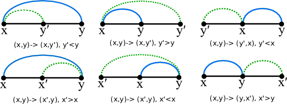
Figure 1: Illustration of shift moves, taken from [6].

RNA secondary structure is known to form a scaffold for tertiary structure formation [5]. Moreover, secondary structure can be efficiently predicted with reasonable accuracy by using either machine learning with stochastic context-free grammars [23, 35, 39], provided that the training set is sufficiently large and representative, or by using ab initio physics-based models with thermodynamics-based algorithms [27, 25]. Since the latter approach does not depend on any form of homology modeling, it has been successfully used for synthetic RNA molecular design [47, 9, 16], to predict microRNA binding sites [32], to discover noncoding RNA genes [44], in simulations to study molecular evolution [3, 42, 36, 15] and in folding kinetics [13, 45, 37, 11]. Software to simulate RNA secondary structure folding kinetics, such as Kinfold and KFOLD, implement the Gillespie algorithm to simulate the moves from one structure to another, for a particular move set. At the elementary-step resolution, two move sets have extensively been studied – the move set $MS_{1}$ which allows the addition or removal of a single base pair, and the move set $MS_{2}$, which allows the addition, removal or shift of a single base pair, where a shift move modifies only one of the two positions in a base pair, as shown in Figure 1.

In simulation studies related to RNA secondary structure evolution, the structural distance between two secondary structures $s,t$ is often measured by the base pair distance, denoted $d_{BP}(s,t)$, defined to be the cardinality of the symmetric difference, $|s\bigtriangleup t|=|s-t|+|t-s|$, i.e. the number of base pairs belonging to $s$ but not $t$, plus the number of base pairs belonging to $t$ but not $s$. In studies concerning RNA folding kinetics, the fast, near-optimal algorithm RNAtabupath [10] and the much slower, but exact (optimal) Barriers algorithm [25] can be used to determine $MS_{1}$ folding trajectories that minimize the barrier energy, defined as the maximum of the (Turner) free energy difference between an intermediate structure and the initial structure. Thermodynamics-based software such as Kinfold, RNAtabupath, and KFOLD use the nearest neighbor free energy model [41] whose energy parameters are inferred from optical melting experiments. In contrast, the two theorems below concern the Nussinov energy model [29], which assigns $-1$ per base pair and ignores entropy. Folding trajectories $s=s_{0},s_{1},\ldots,s_{m}=t$ from $s$ to $t$ may either be direct, whereby each intermediate structure $s_{i}$ is required to contain only base pairs from $s\cup t$, or indirect, without this restriction. Note that indirect pathways may be energetically more favorable, though longer, than direct pathways, and that the problem of constructing an energetically optimal direct folding pathway is NP-hard. Indeed, the following theorem is proven in [40].

Theorem 1 (Maňuch et al. [40]).

With respect to the Nussinov energy model, it is NP-hard to determine, for given secondary structures $s,t$ and integer $k$, whether there exists a direct $MS_{1}$ folding trajectory from $s$ to $t$ with energy barrier at most $k$.

By an easy construction, we can show an analogous result for $MS_{2}$ folding pathways. First, we define a direct $MS_{2}$ folding pathway from secondary structure $s$ to secondary structure $t$ to be a folding pathway $s=s_{0},s_{1},\ldots,s_{n}=t$ where each intermediate structure $s_{i}$ is obtained from $s_{i-1}$ by removing a base pair that belongs to $s$, adding a base pair that belongs to $t$, or shifting a base pair belonging to $s$ into a base pair belonging to $t$.

Theorem 2.

With respect to the Nussinov energy model, it is NP-hard to determine, for given secondary structures $s,t$ and integer $k$, whether there exists a direct $MS_{2}$ folding trajectory from $s$ to $t$ with energy barrier at most $k$.

Proof.

Given secondary structures $s,t$ for an RNA sequence ${\bf a}=a_{1},\ldots,a_{n}$, without loss of generality we can assume that $s,t$ share no common base pair (otherwise, a minimum energy folding trajectory for $s-(s\cap t)$ and $t-(s\cap t)$ yields a minimum energy folding trajectory for $s,t$.) Define the corresponding secondary structures

$$s^{\prime} =\{(2i,2j):(i,j)\in s\}$$

$$t^{\prime} =\{(2i-1,2j-1):(i,j)\in t\}$$

$$a^{\prime}_{2i} =a_{i}=a^{\prime}_{2i-1}\quad\mbox{ for each $1\leq i\leq n$}$$

$${\bf a^{\prime}} =a^{\prime}_{1},a^{\prime}_{2},\ldots,a^{\prime}_{2n}$$

In other words, the sequence ${\bf a^{\prime}}=a_{1},a_{1},a_{2},a_{2},\ldots,a_{n},a_{n}$ is obtained by duplicating each nucleotide of ${\bf a}$, and placing each copy beside the original nucleotide; $s^{\prime}$ [resp. $t^{\prime}$] is obtained by replacing each base pair $(i,j)\in s$ by the base pair $(2i,2j)\in s^{\prime}$ [resp. $(2i-1,2j-1)\in t^{\prime}$. Since there are no base-paired positions that are shared between $s^{\prime}$ and $t^{\prime}$, no shift moves are possible, thus any direct $MS_{2}$ folding pathway from $s^{\prime}$ to $t^{\prime}$ immediately yields a corresponding direct $MS_{1}$ folding pathway from $s$ to $t$. Since the Nussinov energy of any secondary structure equals $-1$ times the number of base pairs, it follows that barrier energy of the direct $MS_{2}$ pathway from $s^{\prime}$ to $t^{\prime}$ is identical to that of the corresponding direct $MS_{1}$ pathway from $s$ to $t$. Since $MS_{1}$ direct barrier energy is an NP-hard problem by Theorem 1, it now follows that the $MS_{2}$ barrier energy problem is NP-hard. ∎

Shift moves, depicted in Figure 1, naturally model both helix zippering and defect diffusion, depicted in Figure 2 and described in [31]. However, shift moves have rarely been considered in the literature, except in the context of folding kinetics [13]. For instance, presumably due to the absence of any method to compute $MS_{2}$ distance, Hamming distance is used as a proxy for $MS_{2}$ distance in the work on molecular evolution of secondary structures appearing in [36] – see also [43], where Hamming distance is used to quantify structural diversity in defining phenotypic plasticity.

In this paper, we introduce the first algorithms to compute the $MS_{2}$ distance between two secondary structures. Although $MS_{1}$ distance, also known as base pair distance, is trivial to compute, we conjecture that $MS_{2}$ distance is NP-hard, where this problem can be formalized as the problem to determine, for any given secondary structures $s,t$ and integer $m$, whether there is an $MS_{2}$ trajectory $s=s_{0},s_{1},\ldots,s_{m}=t$ of length $\leq m$. We describe an optimal (exact, but possibly exponential time) integer programming (IP) algorithm, a fast, near-optimal algorithm, an exact branch-and-bound algorithm, and a greedy algorithm. Since our algorithms involve the feedback vertex set problem for RNA conflict digraphs, we now provide a bit of background on this problem.

Throughout, we are exclusively interested in directed graphs, or digraphs, so unless otherwise indicated, all graphs are assumed to be directed. Any undefined graph-theoretic concepts can be found in the monograph by Bang-Jensen and Gutin [1]. Given a directed graph $G=(V,E)$, a feedback vertex set (FVS) is a subset $V^{\prime}\subseteq V$ which contains at least one vertex from every directed cycle in $G$, thus rendering $G$ acyclic. Similarly, a feedback arc set (FAS) is a subset $E^{\prime}\subseteq E$ which contains at least one directed edge (arc) from every directed cycle in $G$. The FVS [resp. FAS] problem is the problem to determine a minimum size feedback vertex set [resp. feedback arc set] which renders $G$ acyclic. The FVS [resp. FAS] problem can be formulated as a decision problem as follows. Given an integer $k$ and a digraph $G=(V,E)$, determine whether there exists a subset $V^{\prime}\subseteq V$ of size $\leq k$ [resp. $E^{\prime}\subseteq E$ of size $\leq k$], such that every directed cycle contains a vertex in $V^{\prime}$ [resp. an edge in $E^{\prime}$].

In Proposition 10.3.1 of [1], it is proved that FAS and FVS have the same computational complexity, within a polynomial factor. In Theorem 10.3.2 of [1], it is proved that the FAS problem is NP-complete – indeed, this problem appears in the original list of 21 problems shown by R.M. Karp to be NP-complete [22]. Note that Proposition 10.3.1 and Theorem 10.3.2 imply immediately that the FVS problem is NP-complete. In Theorem 10.3.3 of [1], it is proved that the FAS problem is NP-complete for tournaments, where a tournament is a digraph $G=(V,E)$, such that there is a directed edge from $x$ to $y$, or from $y$ to $x$, for every pair of distinct vertices $x,y\in V$. In [30], it is proved that the FAS for Eulerian digraphs is NP-complete, where an Eulerian digraph is characterized by the property that the in-degree of every vertex equals its out-degree. In Theorem 10.3.15 of [1], it is proved that FAS can be solved in polynomial time for planar digraphs, a result originally due to [26]. In [33], a polynomial time algorithm is given for the FAS for reducible flow graphs, a type of digraph that models programs without any GO TO statements (see [19] for a characterization of reducible flow graphs). There is a long history of work on the feedback vertex set and feedback arc set problems, both for directed and undirected graphs, including results on computational complexity as well as exact and approximation algorithms for several classes of graphs – see the survey [12] for an overview of such results.

The plan of the paper is now as follows. In Section 2, we present the graph-theoretic framework for our overall approach and describe a simple, fast algorithm to compute the pseudoknotted $MS_{2}$ distance, or pk-$MS_{2}$ distance, between structures $s,t$. By this we mean the minimum length of an $MS_{2}$ folding trajectory between $s$ and $t$, if intermediate pseudoknotted structures are allowed. We show that the pk-$MS_{2}$ distance between $s$ and $t$, denoted by $d_{pk-MS_{2}}(s,t)$, is approximately equal to one-half the Hamming distance $d_{H}(s,t)$ between $s$ and $t$. This result can be seen as justification, ex post facto, for the use of Hamming distance in the investigation of RNA molecular evolution [36]. In Section 3, we describe an exact integer programming (IP) algorithm which enumerates all directed cycles, then solves the feedback vertex problem for the collection of RNA conflict digraphs, as described in Section 3.1. Our IP algorithm is not a simple reduction to the feedback vertex set (FVS) problem; however, since the complexity of FVS/FAS is known for certain classes of digraphs, we take initial steps towards the characterization of RNA conflict digraphs. Our optimal IP algorithm is much faster than a branch-and-bound algorithm, but it can be too slow to be practical to determine $MS_{2}$ distance between the minimum free energy (MFE) secondary structure and a (Zuker) suboptimal secondary structure for some sequences from the Rfam database [28]. For this reason, in Section 4 we present a fast, near-optimal algorithm, and in Section 5, we present benchmarking results to compare various algorithms of the paper.

Since we believe that further study of RNA conflict digraphs may lead to a solution of the question whether $MS_{2}$ distance is NP-hard, in Appendix A, all types of directed edge that are possible in an RNA conflict digraph are depicted. Appendix B presents details on minimum length pseudoknotted $MS_{2}$ folding pathways, used to provide a lower bound in the branch-and-bound algorithm of Appendix C. Appendix D presents pseudocode for a greedy algorithm.

All algorithms described in this paper have been implemented in Python, and are publicly available at bioinformatics.bc.edu/clotelab/MS2distance. Our software uses the function simple_cycles(G) from the software NetworkX https://networkx.github.io/documentation/networkx-1.9/reference/generated/networkx.algorithms.cycles.simple_cycles.html, and the integer programming (IP) solver Gurobi Optimizer version 6.0 http://www.gurobi.com,2014.

2 $MS_{2}$ distance between possibly pseudoknotted structures

In this section, we describe a straightforward algorithm to determine the $MS_{2}$-distance $d_{pk-MS_{2}}(s,t)$ between any two structures $s,t$ of a given RNA sequence $a_{1},\ldots,a_{n}$, where $d_{pk-MS_{2}}(s,t)$ is defined to be length of a minimal length trajectory $s=s_{0},s_{1},\ldots,s_{m}=t$, where intermediate structures $s_{i}$ may contain pseudoknots, but do not contain any base triples. This variant is called pk-$MS_{2}$ distance. Clearly, the pk-$MS_{2}$ distance is less than or equal to the $MS_{2}$ distance. The purpose of this section is primarily to introduce some of the main concepts used in the remainder of the paper. Although the notion of secondary structure is well-known, we give three distinct but equivalent definitions, that will allow us to overload secondary structure notation to simplify presentation of our algorithms.

Definition 3 (Secondary structure as set of ordered base pairs).

Let $[1,n]$ denote the set $\{1,2,\ldots,n\}$. A secondary structure for a given RNA sequence $a_{1},\ldots,a_{n}$ of length $n$ is defined to be a set $s$ of ordered pairs $(i,j)$, with $1\leq i<j\leq n$, such that the following conditions are satisfied.

1. Watson-Crick and wobble pairs: If $(i,j)\in s$, then $a_{i}a_{j}\in\{GC,CG,AU,UA,GU,UG\}$.

2. No base triples: If $(i,j)$ and $(i,k)$ belong to $s$, then $j=k$; if $(i,j)$ and $(k,j)$ belong to $s$, then $i=k$.

3. Nonexistence of pseudoknots: If $(i,j)$ and $(k,\ell)$ belong to $s$, then it is not the case that $i<k<j<\ell$.

4. Threshold requirement for hairpins: If $(i,j)$ belongs to $s$, then $j-i>\theta$, for a fixed value $\theta\geq 0$; i.e. there must be at least $\theta$ unpaired bases in a hairpin loop. Following standard convention, we set $\theta=3$ for steric constraints.

Without risk of confusion, it will be convenient to overload the concept of secondary structure $s$ with two alternative, equivalent notations, for which context will determine the intended meaning.

Definition 4 (Secondary structure as set of unordered base pairs).

A secondary structure $s$ for the RNA sequence $a_{1},\ldots,a_{n}$ is a set of unordered pairs $\{i,j\}$, with $1\leq i,j\leq n$, such that the corresponding set of ordered pairs

$$\{i,j\}_{<}\stackrel{{\scriptstyle\mbox{\small def}}}{{=}}(\min(i,j),\max(i,j))$$ (1)

satisfies Definition 3.

Definition 5 (Secondary structure as an integer-valued function).

A secondary structure $s$ for $a_{1},\ldots,a_{n}$ is a function $s:[1,\ldots,n]\rightarrow[0,\ldots,n]$, such that $\Big{\{}\{i,s[i]\}_{<}:1\leq i\leq n,s[i]\neq 0\Big{\}}$ satisfies Definition 3; i.e.

$$s[i]=\left\{\begin{array}[]{ll}0&\mbox{if $i$ is unpaired in $s$}\\ j&\mbox{if $(i,j)\in s$ or $(j,i)\in s$}\\ \end{array}\right.$$ (2)

Definition 6 (Secondary structure distance measures).

Let $s,t$ be secondary structures of length $n$. Base pair distance is defined by equation (3) below, and Hamming distance is defined by equation (4) below.

$$d_{BP}(s,t) =|\{(x,y):\left((x,y)\in s\land(x,y)\not\in t\right)\lor\left((x,y)\in t\land(x,y)\not\in s\right)\}|$$ (3)

$$d_{H}(s,t) =|\{i\in[1,n]:s[i]\neq t[i]\}|$$ (4)

Throughout this section, the term pseudoknotted structure is taken to mean a set of ordered pairs [resp. unordered pairs resp. function], which satisfies conditions 1,2,4 (but not necessarily 3) of Definition 3. Given structure $s$ on RNA sequence $\{a_{1},\ldots,a_{n}\}$, we say that a position $x\in[1,n]$ is touched by $s$ if $x$ belongs to a base pair of $s$, or equivalently $s[x]\neq 0$. For possibly pseudoknotted structures $s,t$ on $\{a_{1},\ldots,a_{n}\}$, we partition the set $[1,n]$ into disjoint sets $A$,$B$,$C$,$D$ as follows. Let $A$ be the set of positions that are touched by both $s$ and $t$, yet do not belong to the same base pair in $s$ and $t$, so

$$A =\{i\in[1,n]:s[i]\neq 0,t(i)\neq 0,s[i]\neq t[i]\}$$ (5)

Let $B$ be the set of positions that are touched by either $s$ or $t$, but not by both, so

$$B =\{i\in[1,n]:\left(s[i]\neq 0,t[i]=0\right)\lor\left(s[i]=0,t[i]\neq 0\right)\}$$ (6)

Let $C$ be the set of positions touched by neither $s$ nor $t$, so

$$C =\{i\in[1,n]:s[i]=0=t[i]\}$$ (7)

Let $D$ be the set of positions that belong to the same base pair in both $s$ and $t$, so

$$D =\{i\in[1,n]:s[i]\neq 0,t[i]\neq 0,s[i]=t[i]\}$$ (8)

We further partition $A\cup B$ into a set of maximal paths and cycles, in the following manner. Define an undirected, vertex-colored and edge-colored graph $G=(V,E)$, whose vertex set $V$ is equal to the set $A\cup B$ of positions that are touched by either $s$ or $t$, but not by a common base pair in $(s\cap t)$, and whose edge set $E=(s-t)\cup(t-s)=(s\cup t)-(s\cap t)$ consists of undirected edges between positions that are base-paired together. Color edge $\{x,y\}$ green if the base pair $(x,y)\in s-t$ and red if $(x,y)\in t-s$. Color vertex $x$ yellow if $x$ is incident to both a red and green edge, green if $x$ is incident to a green edge, but not to any red edge, red if $x$ is incident to a red edge, but not to any green edge. The connected components of $G$ can be classified into 4 types of (maximal) paths and one type of cycle (also called path of type 5): type 1 paths have two green end nodes, type 2 paths have a green end node $x$ and a red end node $y$, where $x<y$, type 3 paths have a red end node $x$ and a green end node $y$, where $x<y$, type 4 paths have two red end nodes, and type 5 paths (cycles) have no end nodes. These are illustrated in Figure 3. Note that all nodes of a cycle and interior nodes of paths of type 1-4 are yellow, while end nodes (incident to only one edge) are either green or red. If $X$ is a connected component of $G$, then define the restriction of $s$ [resp. $t$] to $X$, denoted by $s\upharpoonright{X}$ [resp. $t\upharpoonright{X}$], to be the set of base pairs $(i,j)$ in $s$ [resp. $t$] such that $i,j\in X$. With this description, most readers will be able to determine a minimum length pseudoknotted folding pathway from $s\upharpoonright{X}$ to $t\upharpoonright{X}$, where $X$ is a connected component of $G$. For instance, if $X$ is a path of type 2 or 3, then a sequence of shift moves transforms $s\upharpoonright{X}$ into $t\upharpoonright{X}$, beginning with a shift involving the terminal green node. Further details can be found in Appendix B. The formal definitions given below are necessary to provide a careful proof of the relation between Hamming distance and pseudoknotted $MS_{2}$ distance, also found in Appendix B.

Definition 7.

Let $s,t$ be (possibly pseudoknotted) structures on the RNA sequence $a_{1},\ldots,a_{n}$. For $i,j\in[1,n]$, define $i\sim j$ if $s[i]=j$ or $t[i]=j$, and let $\equiv$ be the reflexive, transitive closure of $\sim$. Thus $i\equiv j$ if $i=j$, or $i=i_{1}\sim i_{2}\sim\cdots\sim i_{m}=j$ for any $m\geq 1$. For $i\in[1,n]$, let $[i]$ denote the equivalence class of $i$, i.e. $[i]=\{j\in[1,n]:i\equiv j\}$.

It follows that $i\equiv j$ if and only if $i$ is connected to $j$ by an alternating red/green path or cycle. The equivalence classes $X$ with respect to $\equiv$ are maximal length paths and cycles, as depicted in Figure 3. Moreover, it is easy to see that elements of $A$ either belong to cycles or are found at interior nodes of paths, while elements of $B$ are found exclusively at the left or right terminal nodes of paths.

Note that odd-length cycles cannot exist, due to the fact that a structure cannot contain base triples – see condition 2 of Definition 3. Moreover, even-length cycles can indeed exist – consider, for instance, the structure $s$, whose only base pairs are $(1,15)$ and $(5,10)$, and the structure $t$, whose only base pairs are $(1,5)$ and $(10,15)$. Then we have the red/green cycle $1\rightarrow 5\rightarrow 10\rightarrow 15\rightarrow 1$, consisting of red edge $1\rightarrow 5$, since $(1,5)\in t$, green edge $5\rightarrow 10$, since $(5,10)\in s$, red edge $10\rightarrow 15$, since $(10,15)\in t$, and green edge $15\rightarrow 1$, since $(1,15)\in s$.

From the discussion before Definition 7, it follows that $A$ in equation (5) consists of the nodes of every cycle together with all interior (yellow) nodes of paths of type 1-4. Moreover, we can think of $B$ in equation (6) as consisting of all path end nodes, i.e. those that have only one incident edge. Let $B_{1}\subseteq B$ [resp. $B_{2}\subseteq B$] denote the set of elements of $B$ that belong to type 1 paths [resp. type 4 paths] of length 1, i.e. positions incident to isolated green [resp. red] edges that correspond to base pairs $(i,j)\in s$ where $i,j$ are not touched by $t$ [resp. $(i,j)\in t$ where $i,j$ are not touched by $s$]. Let $B_{0}=B-B_{1}-B_{2}$ be the set of end nodes of a path of length 2 or more. Letting $BP_{1}$ [resp. $BP_{2}$] denote the set of base pairs $(i,j)$ that belong to $s$ and are not touched by $t$ [resp. belong to $t$ and are not touched by $s$], we can formalize the previous definitions as follows.

$$B_{1} =\{i\in[1,n]:\exists j\left[\{i,j\}\in s,t(i)=0=t(j)\right]$$ (9)

$$B_{2} =\{i\in[1,n]:\exists j\left[\{i,j\}\in t,s(i)=0=s(j)\right]$$ (10)

$$B_{0} =B-(B_{1}\cup B_{2})$$ (11)

$$BP_{1} =\{(i,j)\in s:t[i]=0=t[j]\}$$ (12)

$$BP_{2} =\{(i,j)\in t:s[i]=0=s[j]\}$$ (13)

In Appendix B, it is proved that pk-$MS_{2}$ distance between $s\upharpoonright{X}$ and $t\upharpoonright{X}$ for any maximal path $X$ is equal to Hamming distance $\lfloor\frac{d_{H}(s\upharpoonright{X},t\upharpoonright{X})}{2}\rfloor$; in contrast, pk-$MS_{2}$ distance between $s\upharpoonright{X}$ and $t\upharpoonright{X}$ for any cycle $X$ is equal to $\lfloor\frac{d_{H}(s\upharpoonright{X},t\upharpoonright{X})}{2}\rfloor+1$. It follows that

$$d_{pk-MS_{2}}(s,t) =\lfloor\frac{d_{H}(s,t)}{2}\rfloor$$ (14)

if and only if there are no type 5 paths (i.e. cycles). This result justifies ex post facto the use of Hamming distance in the investigation of RNA molecular evolution [36, 43]. We also have the following.

Lemma 8.

Let $s,t$ be two arbitrary (possibly pseudoknotted) structures for the RNA sequence $a_{1},\ldots,a_{n}$, and let $X_{1},\ldots,X_{m}$ be the equivalence classes with respect to equivalence relation $\equiv$ on $A\cup B$. Then the pk-$MS_{2}$ distance between $s$ and $t$ is equal to

$$d_{pk-MS_{2}}(s,t) =\sum_{i=1}^{m}\max\Big{(}|s\upharpoonright{X_{i}}|,|t\upharpoonright{X_{i}}|\Big{)}$$

This lemma is useful, since the pk-$MS_{2}$ distance provides a lower bound for the $MS_{2}$ distance between any two secondary structures, and hence allows a straightforward, but slow (exponential time) branch-and-bound algorithm to be implemented for the exact $MS_{2}$ distance – pseudocode for the branch-and-bound algorithm is given in Section C of the Appendix. To compute pk-$MS_{2}$ distance, we remove those base pairs in $s-t$ that are not touched by $t$, compute the equivalence classes (connected components) $X$ on the set of positions belonging to the remaining base pairs (provided that the position does not belong to a common base pair of both $s$ and $t$), then determine for each $X$ a minimum length pk-$MS_{2}$ folding pathway from $s\upharpoonright{X}$ to $t\upharpoonright{X}$. The formal pseudocode follows.

Algorithm 9 (pk-$MS_{2}$ distance).

$MS_{2}$-path length between two possibly pseudoknotted structures $s,t$.

1. remove from $s$ all base pairs of $BP_{1}$

2. $numMoves=|BP_{1}|$

3. $Q=A\cup B_{0}$

4. while $Q\neq\emptyset$ {

5. $x_{0}=\min(Q)$; $X=[x_{0}]$ //$X$ is equivalence class of $x_{0}$

6. determine path type of $X$

7. compute minimum length folding pathway from $s\upharpoonright{X}$ to $t\upharpoonright{X}$

8. $numMoves=numMoves+\max(|s\upharpoonright{X}|,|t\upharpoonright{X}|)$

9. add to $s$ all base pairs in $BP_{2}$

10. $numMoves=numMoves+|BP_{2}|$

11. return $numMoves$

Straightforward details of how to implement line 7 are given in the Appendix. The principle underlying the reason that Algorithm 9 produces a minimum length (pseudoknotted) $MS_{2}$ folding trajectory from $s$ to $t$ is that we maximize the number of shift moves, since a single shift move from $\{x,y\}\in s$ to $\{y,z\}\in t$ corresponds to the simultaneous removal of $\{x,y\}$ and addition of $\{y,z\}$. We apply this principle in the next section to determine the minimum length (non-pseudoknotted) $MS_{2}$ folding trajectory from $s$ to $t$.

3 $MS_{2}$ distance between secondary structures

In this section, we present an integer programming (IP) algorithm to compute the $MS_{2}$ distance between any two secondary structures $s,t$, i.e. the minimum length of an $MS_{2}$ trajectory from $s$ to $t$. Our algorithm has been cross-checked with the exhaustive branch-and-bound algorithm mentioned at the end of the last section.

As in the previous section, our goal is to maximize the number of shift operations in the $MS_{2}$ trajectory, formalized in the following simple theorem, whose proof is clear.

Theorem 10.

Suppose that the $MS_{2}$ distance between secondary structures $s,t$ is $k$, i.e. base pair distance $d_{BP}(s,t)=|s-t|+|t-s|=k$. Suppose that $\ell$ is the number of shift moves occurring in a minimum length $MS_{2}$ refolding trajectory $s=s_{0},s_{1},\ldots,s_{m}=t$ from $s$ to $t$. Then the $MS_{2}$ distance between $s$ and $t$ equals

$$d_{MS_{2}}(s,t)=\ell+(k-2\ell)=k-\ell$$ (15)

Our strategy will now be to use a graph-theoretic approach to maximize the number of shift moves.

3.1 RNA conflict digraph

Throughout this section, we take $s,t$ to be two arbitrary, distinct, but fixed secondary structures of the RNA sequence $a_{1},\ldots,a_{n}$. Recall the definitions of $A,B,C,D$ in equations (5–8), so that $A$ is the set of positions $x\in[1,n]$ that are base-paired in both $s$ and $t$, but the base pairs in $s$ and $t$ are not identical; $B$ is the set of positions $x\in[1,n]$ that are base-paired in one of $s$ or $t$, but not both; $C$ is the set of positions $x\in[1,n]$ that are base-paired in neither $s$ nor $t$, and $D$ is the set of positions $x\in[1,n]$ that are base-paired to the same partner in both $s$ and $t$.

To determine a minimum length $MS_{2}$ folding trajectory from secondary structure $s$ to secondary structure $t$ is to maximize the number of shift moves and minimize the number of base pair additions and removals. To that end, note that the base pairs in $s$ that do not touch any base pair of $t$ must be removed in any $MS_{2}$ path from $s$ to $t$, since there is no shift of such base pairs to a base pair of $t$ – such base pairs are exactly those in $BP_{1}$, defined in equation (12). Similarly, note that the base pairs in $t$ that do not touch any base pair of $s$ must occur must be added, in the transformation of $s$ to $t$, since there is no shift of any base pair from s to obtain such base pairs of $t$ – such base pairs are exactly those in $BP_{2}$, defined in equation (13). We now focus on the remaining base pairs of $s$, all of which touch a base pair of $t$, and hence could theoretically allow a shift move in transforming $s$ to $t$, provided that there is no base triple or pseudoknot introduced by performing such a shift move. Examples of all six possible types of shift move are illustrated in Figure 4. To handle such cases, we define the notion of RNA conflict digraph, solve the feedback vertex set (FVS) problem [22] by integer programming (IP), apply topological sorting [7] to the acyclic digraph obtained by removing a minimum set of vertices occurring in feedback loops, then apply shift moves in topologically sorted order. We now formalize this argument.

Define the digraph $G=(V,E)$, whose vertices (or nodes) $n\in V$ are defined in the following Definition 11 and whose directed edges are defined in Definition 12.

Definition 11 (Vertex in an RNA conflict digraph).

If $s,t$ are distinct secondary structures for the RNA sequence $a_{1},\ldots,a_{n}$, then a vertex in the RNA conflict digraph $G=G(s,t)$ is a triplet node, or more simply, node $v=(x,y,z)$ consisting of integers $x,y,z$, such that the base pair $\{x,y\}_{<}=(\min(x,y),\max(x,y))$ belongs to $t$, and the base pair $\{y,z\}_{<}=(\min(y,z),\max(y,z))$ belongs to $s$. Let $v.t$ [resp. $v.s$] denote the base pair $\{x,y\}_{<}$ [resp. $\{y,z\}_{<}$] belonging to $t$ [resp. $s$]. The middle integer $y$ of node $v=(x,y,z)$ is called the pivot position, since it is common to both $s$ and $t$. Nodes are ordered by the integer ordering of their pivot positions: $(x,y,z)\preceq(x^{\prime},y^{\prime},z^{\prime})$ if and only if $y\leq y^{\prime}$ (or $y=y^{\prime}$ and $x<x^{\prime}$, or $y=y^{\prime}$, $x=x^{\prime}$, and $z<z^{\prime}$). If $v=(x,y,z)$ is a node, then $flatten(v)$ is defined to be the set $\{x,y,z\}$ of its coordinates.

Nodes are representations of a potential shift move, and can be categorized into six types, as shown in Figure 4.

Definition 12 (Directed edge in an RNA conflict digraph).

Base pairs $\{a,b\}_{<}$ and $\{c,d\}_{<}$ are said to touch if $|\{a,b\}\cap\{c,d\}|=1$; in other words, base pairs touch if they form a base triple. Base pairs $\{a,b\}_{<}$ and $\{c,d\}_{<}$ are said to cross if either $\min(a,b)<\min(c,d)<\max(a,b)<\max(c,d)$ or $\min(c,d)<\min(a,b)<\max(c,d)<\max(a,b)$; in other words, base pairs cross if they form a pseudoknot. There is a directed edge from node $n_{1}=(x_{1},y_{1},z_{1})$ to node $n_{2}=(x_{2},y_{2},z_{2})$, denoted by $(n_{1},n_{2})\in E$ or equivalently by $n_{1}\rightarrow n_{2}$, if (1) $|flatten(n_{1})\cap flatten(n_{2})|\leq 1$, or in other words if $n_{1}$ and $n_{2}$ overlap in at most one position, and (2) the base pair $\{y_{1},z_{1}\}_{<}\in s$ from $n_{1}$ either touches or crosses the base pair $\{x_{2},y_{2}\}_{<}\in t$ from $n_{2}$.

Note that if the base pair $\{y_{1},z_{1}\}_{<}\in s$ from $n_{1}$ touches the base pair $\{x_{2},y_{2}\}_{<}\in t$ from $n_{2}$, then it must be that $z_{1}=x_{2}$; indeed, since each pivot node $y_{1}$ [resp. $y_{2}$] belongs to a base pair of both $s$ and $t$, it cannot be that $z_{1}=y_{2}$ (because then $\{y_{1},z_{1}\}_{<}\in s$ and $\{y_{2},z_{2}\}_{<}\in s$ would form a base triple in $s$ at $z_{1}=y_{2}$), nor can it be that $y_{1}=x_{2}$ (because then $\{x_{1},y_{1}\}_{<}\in t$ and $\{x_{2},y_{2}\}_{<}\in t$ would form a base triple in $t$ at $y_{1}=x_{2}$). Note as well that if $n_{1}=(x_{1},y_{1},z_{1})$ and $n_{2}=(x_{2},y_{2},z_{2})$ are triplet nodes, then $|flatten(n_{1})\cap flatten(n_{2})|=1$ implies that either $n_{1}\rightarrow n_{2}$ or $n_{2}\rightarrow n_{1}$. Indeed, if there is a common element shared by $n_{1}$ and $n_{2}$, then it cannot be a pivot element, since $s$ and $t$ cannot have a base triple. For the same reason, the common element cannot belong to the base pairs $\{x_{1},y_{1}\}\in t$ of $n_{1}$ and $\{x_{2},y_{2}\}\in t$ of $n_{2}$ (otherwise $t$ would contain a base triple), nor can the common element belong to the base pairs $\{y_{1},z_{1}\}\in s$ of $n_{1}$ and $\{y_{2},z_{2}\}\in s$ of $n_{2}$ (otherwise $s$ would contain a base triple). It follows that either $\{x_{1},y_{1}\}\cap\{y_{2},z_{2}\}\neq\emptyset$, or $\{x_{2},y_{2}\}\cap\{y_{1},z_{1}\}\neq\emptyset$. From the assumption that $|flatten(n_{1})\cap flatten(n_{2})|=1$, this implies that either $n_{2}\rightarrow n_{1}$ or that $n_{1}\rightarrow n_{2}$, but not both. Finally, note that if $n_{1}=(x_{1},y_{1},z_{1})$, $n_{2}=(x_{2},y_{2},z_{2})$ and $|flatten(n_{1})\cap flatten(n_{2})|=2$, then there are exactly three possibilities, all of which can be realized:

1. $n_{1}.t=n_{2}.t$, so that $\{x_{1},y_{1}\}=\{x_{2},y_{2}\}$, as in the example $(1,5)\in s$, $(10,15)\in s$, $(5,10)\in t$, $n_{1}=(10,5,1)$, $n_{2}=(5,10,15)$;

2. $n_{1}.s=n_{2}.s$, so that $\{y_{1},z_{1}\}=\{y_{2},z_{2}\}$, as in the example $(1,5)\in t$, $(10,15)\in t$, $(5,10)\in s$, $n_{1}=(1,5,10)$, $n_{2}=(15,10,5)$;

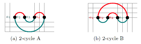
Figure 5: Two special types of closed 2-cycles. (a) RNA conflict digraph $G=(V,E)$ for secondary structures $t$ and $s$, where $a_{1}<a_{2}<a_{3}<a_{4}$ and $t=\{(a_{1},a_{2}),(a_{3},a_{4})\}$, and $s=\{(a_{1},a_{4}),(a_{2},a_{3})\}$. Nodes of $V=\{v_{1},v_{2},v_{3},v_{4}\}$ are the following: $v_{1}=(a_{1},a_{2},a_{3})$ of type 1, $v_{2}=(a_{3},a_{4},a_{1})$ of type 5, $v_{3}=(a_{2},a_{1},a_{4})$ of type 4, and $v_{4}=(a_{4},a_{3},a_{2})$ of type 2. (b) RNA conflict digraph $G=(V,E)$ for secondary structures $t$ and $s$, where $a_{1}<a_{2}<a_{3}<a_{4}$ and $t=\{(a_{1},a_{4}),(a_{2},a_{3})\}$ and $s=\{(a_{1},a_{2}),(a_{3},a_{4})\}$. Nodes of $V=\{v_{1},v_{2},v_{3},v_{4}\}$ are the following: $v_{1}=(a_{1},a_{4},a_{3})$ of type 6, $v_{2}=(a_{4},a_{1},a_{2})$ of type 3, $v_{3}=(a_{2},a_{3},a_{4})$ of type 1, $v_{4}=(a_{3},a_{2},a_{1})$ of type 2. Since the overlap between any two distinct vertices in (a) and (b) is 2, there are no edges in $E$ for the conflict digraphs of (a) and (b). An optimal trajectory from $s$ to $t$ is constructed by removing a base pair from $s$, performing a shift, and adding the remaining base pair from $t$. In each case there are 2 choices for the base pair to remove and two choices for the shift, so 4 optimal trajectories for each of (a) and (b).

3. $\{x_{1},z_{1}\}=\{x_{2},z_{2}\}$, as shown in Figure 5. This latter example will be called a closed 2-cycle.

These considerations produce the equivalent but sharper following definition.

Definition 13 (Conflict digraph $G=(V,E)$).

Let $s,t$ be distinct secondary structures for the RNA sequence $a_{1},\ldots,a_{n}$. The RNA confict digraph $G(s,t)=(V(s,t),E(s,t))$, or $G=(V,E)$ when $s,t$ are clear from context, is defined by

$$V =\{(x,y,z):x,y,z\in[1,n]\land\{x,y\}\in t\land\{y,z\}\in s\}$$ (16)

$$E =\Big{\{}(n_{1},n_{2}):n_{1}=(x_{1},y_{1},z_{1})\in V\land n_{2}=(x_{2},y_{2},z_{2})\in V\land$$

$$|flatten(n_{1})\cap flatten(n_{2})|\leq 1\land\Big{(}z_{1}=x_{2}\lor$$

$$\Big{(}\left[\min(y_{1},z_{1})<\min(x_{2},y_{2})<\max(y_{1},z_{1})<\max(x_{2},y_{2})\right]\lor$$

$$\left[\min(x_{2},y_{2})<\min(y_{1},z_{1})<\max(x_{2},y_{2})<\max(y_{1},z_{1})\right]\Big{)}\Big{\}}$$ (17)

The set of directed edges of conflict digraph $G=(V,E)$, as defined in Definition 13, establishes a partial ordering on vertices of $V$ with the property that $n_{1}\rightarrow n_{2}$ holds for vertices $n_{1}=(x,y,z)$, $n_{2}=(u,v,w)$ if and only if (1) $n_{1}$ and $n_{2}$ overlap in at most one position, and (2) when shift move $n_{2}$ is applied, shifting $\{v,w\}\in s$ to $\{u,v\}\in t$, the base pair $\{u,v\}$ either touches or crosses the base pair $\{y,z\}\in s$ in $n_{1}$. It follows that if $n_{1}\rightarrow n_{2}$, then the shift move in which $\{y,z\}\in s$ shifts to $\{x,y\}\in t$ must be performed before the shift move where $\{v,w\}\in s$ shifts to $\{u,v\}\in t$ – indeed, if shifts are performed in the opposite order, then after shifting $\{v,w\}\in s$ to $\{u,v\}\in t$ and before shifting $\{y,z\}\in s$ to $\{x,y\}\in t$, we would create either a base triple or a pseudoknot.

Strictly speaking, the overlap condition (1) is not a necessary requirement, and in our first IP algorithm to compute $MS_{2}$ distance [2], we considered a somewhat more general edge relation without condition (1). If distinct vertices $n_{1},n_{2}$ violate condition (1), then $|flatten(n_{1})\cap flatten(n_{2})|=2$, and the constraint (${\ddagger}$) in line 7 of Algorithm 14 would ensure that at most one of $n_{1},n_{2}$ are selected by the IP solver for the set $\overline{V}$, in the resulting acyclic digraph $\overline{G}=(\overline{V},\overline{E})$. Nevertheless, the run time of our algorithm depends heavily on the number of simple directed cycles in the initial conflict digraph $G=(V,E)$. Without condition (1), nodes $n_{1},n_{2}$ in a closed 2-cycle (see Figure 5) satisfy $n_{1}\rightarrow n_{2}$ and $n_{2}\rightarrow n_{1}$. Since it is possible that $n_{1}$ belong to other cycles that do not contain $n_{2}$, this can (and does) lead to a greatly increased number of directed cycles, hence much longer run time – indeed, our algorithm in [2] runs 10 times slower than the current algorithm.

Before proceeding with the description of the algorithm, we must explain how to treat closed 2-cycles, as shown in Figure 5, for which there exist four integers $a_{1}<a_{2}<a_{3}<a_{4}$, such that either Case A or Case B holds.

Case A: Base pairs $(a_{1},a_{2})$ and $(a_{3},a_{4})$ belong to $t$, while base pairs $(a_{1},a_{4})$ and $(a_{2},a_{3})$ belong to $s$, as shown in Figure 5a.

In this case, the conflict digraph $G=(V,E)$ contains the following 4 vertices $v_{1}=(a_{1},a_{2},a_{3})$ of type 1, $v_{2}=(a_{3},a_{4},a_{1})$ of type 5, $v_{3}=(a_{2},a_{1},a_{4})$ of type 4, and $v_{4}=(a_{4},a_{3},a_{2})$ of type 2. The overlap of any two distinct vertices has size 2, so by Definition 13, there can be no directed edge between any vertices. There are four optimal trajectories of size 3; for specificity we select the following optimal trajectory:

remove $$(a_{1},a_{4}) s$$ from (18)

Case B: Base pairs $(a_{1},a_{2})$ and $(a_{3},a_{4})$ belong to $s$, while base pairs $(a_{1},a_{4})$ and $(a_{2},a_{3})$ belong to $t$, as shown in Figure 5b.

In this case, the conflict digraph $G=(V,E)$ contains the following 4 vertices $v_{1}=(a_{1},a_{4},a_{3})$ of type 6, $v_{2}=(a_{4},a_{1},a_{2})$ of type 3, $v_{3}=(a_{2},a_{3},a_{4})$ of type 1, and $v_{4}=(a_{3},a_{2},a_{1})$ of type 2. The overlap of any two distinct vertices has size 2, so by Definition 13, there can be no directed edge between any vertices. There are four optimal trajectories of size 3; for specificity we select the following optimal trajectory:

remove $$(a_{1},a_{2}) s$$ from (19)

In Algorithm 14 below, it is necessary to list all closed 2-cycles, as depicted in Figure 5. This can be done in linear time $O(n)$, for RNA sequence ${\bf a}=a_{1},\ldots,a_{n}$ and secondary structures $s,t$ by computing equivalence classes as defined in Definition 7, then inspecting all size 4 equivalence classes $X=\{a_{1},a_{2},a_{3},a_{4}\}$ to determine whether Case A or Case B applies. For each such closed 2-cycle, Algorithm 14 computes the partial trajectory (18) or (19) appropriately, then the vertices $v_{1},v_{2},v_{3},v_{4}$ are deleted. No edges need to be deleted, since there are no edges between $v_{i}$ and $v_{j}$ for $1\leq i,j\leq 4$. In creating the partial trajectories, the variable numMoves must be updated.

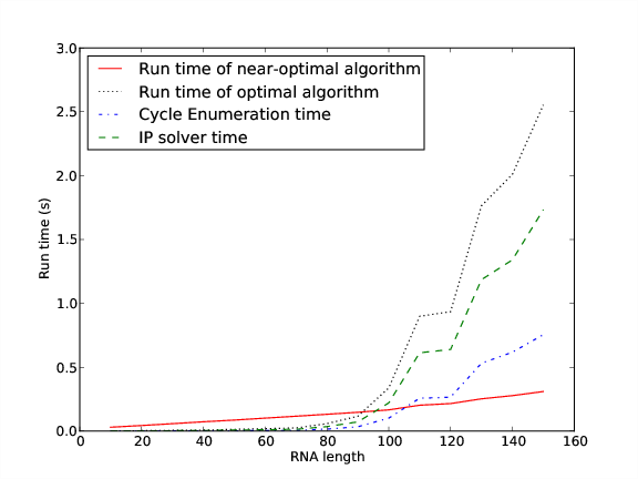
Figure 14: Run time for the exact IP (optimal) algorithm 14 and the near-optimal algorithm 15 to compute minimum length $MS_{2}$ folding trajectories for the same data set from previous Figure 12. Each data point represents the average $\mu\pm\sigma$ where error bars indicate one standard deviation, taken over $71,250$ many sequence/structure pairs. Run time of the optimal algorithm depends on time to perform topological sort, time to enumerate all directed cycles using our Python implementation of Johnson’s algorithm [21], and time for the Gurobi IP solver (ordered here by increasing time demands).

By special treatment of closed 2-cycles, we obtain a 10-fold speed-up in the exact IP Algorithm 14 over that of the precursor Algorithm 10 in our WABI 2017 proceedings paper [2] – compare run times of Figure 14 with those from Figure 5 of [2]. Except for the special case of closed 2-cycles that must be handled before general treatment, note that Definition 13 establishes a partial ordering on vertices of the conflict digraph $G=(V,E)$, in that edges determine the order in which shift moves should be performed. Indeed, if $n_{1}=\{x,y,z\}$, $n_{2}=\{u,v,z\}$ and $(n_{1},n_{2})\in E$, which we denote from now on by $n_{1}\rightarrow n_{2}$, then the shift move in which $\{y,z\}\in s$ shifts to $\{x,y\}\in t$ must be performed before the shift move where $\{v,w\}\in s$ shifts to $\{u,v\}\in t$ – indeed, if shifts are performed in the opposite order, then after shifting $\{v,w\}\in s$ to $\{u,v\}\in t$ and before shifting $\{y,z\}\in s$ to $\{x,y\}\in t$, we would create either a base triple or a pseudoknot. Our strategy to efficiently compute the $MS_{2}$ distance between secondary structures $s$ and $t$ will be to (1) enumerate all simple cycles in the conflict digraph $G=(V,E)$ and to (2) apply an integer programming (IP) solver to solve the minimum feedback arc set problem $V^{\prime}\subset V$. Noticing that the induced digraph $\overline{G}=(\overline{V},\overline{E})$, where $\overline{V}=V-V^{\prime}$ and $\overline{E}=E\cap(\overline{V}\times\overline{V})$, is acyclic, we then (3) topologically sort $\overline{G}$, and (4) perform shift moves from $\overline{V}$ in topologically sorted order.

Algorithm 14 ($MS_{2}$ distance from $s$ to $t$).

Input: Secondary structures $s,t$ for RNA sequence $a_{1},\ldots,a_{n}$ Output: Folding trajectory $s=s_{0},s_{1},\ldots,s_{m}=t$, where $s_{0},\ldots,s_{m}$ are secondary structures, $m$ is the minimum possible value for which $s_{i}$ is obtained from $s_{i-1}$ by a single base pair addition, removal or shift for each $i=1,\ldots,m$.

First, initialize the variable numMoves to $0$, and the list moveSequence to the empty list [ ]. Recall that $BP_{2}=\{(x,y):(x,y)\in t,(s-t)[x]=0,(s-t)[y]=0\}$. Bear in mind that $s$ is constantly being updated, so actions performed on $s$ depend on its current value.

//remove base pairs from $s$ that are untouched by $t$

1. $BP_{1}=\{(x,y):(x,y)\in s,(t-s)[x]=0,(t-s)[y]=0\}$

2. for $(x,y)\in BP_{1}$

3. remove $(x,y)$ from $s$; numMoves = numMoves+1

//define conflict digraph $G=(V,E)$ on updated $s$ and unchanged $t$

4. define $V$ by equation (16)

5. define $E$ by equation (17)

6. define conflict digraph $G=(V,E)$

//IP solution of minimum feedback arc set problem

7. maximize $\sum_{v\in V}x_{v}$ where $x_{v}\in\{0,1\}$, subject to constraints (${\dagger}$) and (${\ddagger}$)

//constraint to remove vertex from each simple cycle of $G$

(${\dagger}$) $\sum\limits_{v\in C}x_{v}<|C|$ for each simple directed cycle $C$ of $G$

//constraint to ensure shift moves cannot be applied if they share same base pair from $s$ or $t$

(${\ddagger}$) $x_{v}+x_{v^{\prime}}\leq 1$, for all pairs of vertices $v=(x,y,z)$ and $v^{\prime}=(x^{\prime},y^{\prime},z^{\prime})$ with $|\{x,y,z\}\cap\{x^{\prime},y^{\prime},z^{\prime}\}|=2$

//define IP solution acyclic digraph $\overline{G}=(\overline{V},\overline{E})$

8. $\overline{V}=\{v\in V:x_{v}=1\}$; $V^{\prime}=\{v\in V:x_{v}=0\}$

9. $\overline{E}=\{(v,v^{\prime}):v,v^{\prime}\in\overline{V}\land(v,v^{\prime})\in E\}$

10. $\overline{G}=(\overline{V},\overline{E})$

//handle special, closed 2-cycles

11. for each closed 2-cycle $[x]=\{a_{1},a_{2},a_{3},a_{4}\}$ as depicted in Figure 5

12. if $[x]$ is of type A as depicted in Figure 5a

13. remove base pair from $s$ by equation (18)

14. if $[x]$ is of type B as depicted in Figure 5b

15. remove base pair from $s$ by equation (19)

//remove base pairs from $s$ that are not involved in a shift move

16. $\overline{V}.s=\{(x,y):\exists v\in\overline{V}(v.s=(x,y))\}$

17. for $(x,y)\in s-t$

18. if $(x,y)\not\in\overline{V}.s$

19. remove $(x,y)$ from $s$; numMoves = numMoves+1

//topological sort for IP solution $\overline{G}=(\overline{V},\overline{E})$

20. topological sort of $\overline{G}$ using DFS [7] to obtain total ordering $\prec$ on $\overline{V}$

21. for $v=(x,y,z)\in\overline{V}$ in topologically sorted order $\prec$

22. shift $\{y,z\}$ to $\{x,y\}$ in $s$; numMoves = numMoves+1

//add remaining base pairs from $t-s$, e.g. from $BP_{2}$ and type 4,5 paths in Figure 3

23. for $(x,y)\in t-s$

24. add $(x,y)$ to $s$; numMoves = numMoves+1

25. return folding trajectory, numMoves

We now illustrate the definitions and the execution of the algorithm for a tiny example where $s=\{(1,5),(10,15),(20,25)\}$ and $t=\{(5,10),(15,20)\}$. From Definition 7, there is only one equivalence class $X=\{1,5,10,15,20,25\}$ and it is a path of type 1, as illustrated in Figure 3, where $b_{1}=1$, $a_{1}=5$, $b2=10$, $a_{2}=15$, $b_{3}=20$, $a_{3}=25$. From Definition 11, there are 4 vertices in the conflict digraph $G=(V,E)$, where $v_{1}=(10,5,1)$, $v_{2}=(5,10,15)$, $v_{3}=(20,15,10)$, $v_{4}=(15,20,25)$ – recall the convention from that definition that vertex $v=(x,y,z)$ means that base pair $\{y,z\}\in s$ and base pair $\{x,y\}\in t$, so that the pivot position $y$ is shared by base pairs from both $s$ and $t$. From Definition 12, there are only two directed edges, $v_{1}\rightarrow v_{3}$ since $v_{1}.s$ touches $v_{2}.t$, and $v_{2}\rightarrow v_{4}$ since $v_{2}.s$ touches $v_{4}.t$. Note there is no edge from $v_{1}$ to $v_{2}$, or from $v_{2}$ to $v_{3}$, or from $v_{3}$ to $v_{4}$, since their overlap has size 2 – for instance $flatten(v_{1})=\{1,5,10\}$, $flatten(v_{2})=\{5,10,15\}$, and $flatten(v_{1})\cap flatten(v_{2})=\{5,10\}$ of size 2. There is no cycle, so the constraint (${\dagger}$) in line 7 of Algorithm 14 is not applied; however the constraint (${\ddagger}$) does apply, so that $x_{v_{1}}+x_{v_{2}}\leq 1$, $x_{v_{2}}+x_{v_{3}}\leq 1$, $x_{v_{3}}+x_{v_{4}}\leq 1$. It follows that there are three possible IP solutions for the vertex set $\overline{V}$.

Case 1: $\overline{V}=\{v_{1},v_{3}\}$ Then $v_{1}.s=(1,5)$, $v_{3}.s=(10,15)$ so $\overline{V}.s=\{(1,5),(10,15)\}$ and by lines 11-14 we remove base pair $(20,25)$ from $s$. Now $\overline{G}=(\overline{V},\overline{E})$, where $\overline{E}=\{v_{1}\rightarrow v_{3}\}$, so topological sort is trivial and we complete the trajectory by applying shift $v_{1}$ and then shift $v_{3}$. Trajectory length is 5.

Case 2: $\overline{V}=\{v_{1},v_{4}\}$ Then $v_{1}.s=(1,5)$, $v_{4}.s=(20,25)$ so $\overline{V}.s=\{(1,5),(20,25)\}$ and by lines 11-14 we remove base pair $(10,15)$ from $s$. Now $\overline{G}=(\overline{V},\overline{E})$, where $\overline{E}=\emptyset$, so topological sort is trivial and we complete the trajectory by applying shift $v_{1}$ and then shift $v_{4}$, or by applying shift $v_{4}$ and then shift $v_{1}$. Trajectory length is 5.

Case 3: $\overline{V}=\{v_{2},v_{4}\}$ Then $v_{2}.s=(10,15)$, $v_{4}.s=(20,25)$ so $\overline{V}.s=\{(10,15),(20,25)\}$ and by lines 11-14 we remove base pair $(1,5)$ from $s$. Now $\overline{G}=(\overline{V},\overline{E})$, where $\overline{E}=\{v_{2}\rightarrow v_{4}\}$, so topological sort is trivial and we complete the trajectory by applying shift $v_{2}$ and then shift $v_{4}$. Trajectory length is 5.

3.2 Examples to illustrate Algorithm 14

We illustrate concepts defined so far with three examples: a toy 20 nt RNA sequence, a 25 nt bistable switch, and the 56 nt spliced leader RNA from L. collosoma.

3.2.1 Toy 20 nt sequence

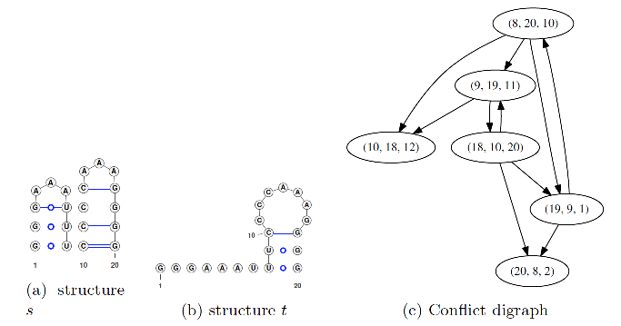
Figure 6: Conflict digraph for a 20 nt toy example with sequence GGGAAAUUUC CCCAAAGGGG, with initial structure $s$ whose free energy is +0.70 kcal/mol, and target structure $t$ whose free energy is + 3.30 kcal/mol. The conflict digraph contains 3 simple cycles: a first cycle $\{(8,20,10),(9,19,11),(18,10,20),(19,9,1)\}$ of size 4, a second cycle $\{[(8,20,10),(19,9,1)\}$ of size 2, and a third cycle $\{(18,10,20),(9,19,11)\}$ of size 2.

For the toy 20 nt sequence GGGAAAUUUC CCCAAAGGGG with initial structure $s$ shown in Figure 6a, and target structure $t$ shown in Figure 6b, the corresponding conflict digraph is shown in Figure 6c. This is a toy example, since the empty structure is energetically more favorable than either structure: free energy of $s$ is +0.70 kcal/mol, while that for $t$ is +3.30 kcal/mol. The conflict digraph contains 6 vertices, 10 directed edges, and 3 simple cycles: a first cycle $\{(8,20,10),(9,19,11),(18,10,20),(19,9,1)\}$ of size 4, a second cycle $\{[(8,20,10),(19,9,1)\}$ of size 2, and a third cycle $\{(18,10,20),(9,19,11)\}$ of size 2.

3.2.2 Bistable switch

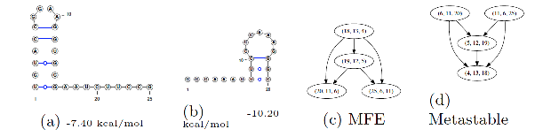
Figure 7: Conflict digraphs for the 25 nt bistable switch with sequence UGUACCGGAA GGUGCGAAUC UUCCG taken from Figure 1(b).1 of [20], in which the authors performed structural probing by comparative imino proton NMR spectroscopy. (a) Minimum free energy (MFE) structure having -10.20 kcal/mol. (b) Alternate metastable structure having next lowest free free energy of -7.40 kcal/mol. Two lower energy structures exist, having -9.00 kcal/mol resp. -7.60 kcal/mol; however, each is a minor variant of the MFE structure. (c) RNA conflict digraph $G=(V,E)$, having directed edges $(x,y,z)\rightarrow(u,v,w)$ if the (unordered) base pair $\{y,z\}\in s$ touches or crosses the (unordered) base pair $\{u,v\}\in t$. Here, $s$ is in the metastable structure shown in (b) having -7.40 kcal/mol, while $t$ is the MFE structure shown in (a) having -10.20 kcal/mol. The conflict digraph represents a necessary order of application of shift moves, in order to avoid the creation of base triples or pseudoknots. Note that the digraph $G$ is acyclic, but the IP solver must nevertheless be invoked with constraint (${\ddagger}$) that precludes both vertices $(20,11,6)$ and $(25,6,11)$ from belonging to the solution $\overline{V}$. (d) RNA conflict digraph $G^{\prime}=(V^{\prime},E^{\prime})$, having similar definition in which roles of $s$ and $t$ are reversed – i.e. $MS_{2}$ folding pathways from the MFE structure to the (higher energy) metastable structure.

Figure 7 depicts the secondary structure for the metastable and the MFE structures, as well as the corresponding conflict digraphs for the 25 nt bistable switch, with sequence UGUACCGGAA GGUGCGAAUC UUCCG, taken from Figure 1(b).1 of [20], in which the authors report structural probing by comparative imino proton NMR spectroscopy. The minimum free energy (MFE) structure has -10.20 kcal/mol, while the next metastable structure has -7.40 kcal/mol. Two lower energy structures exist, having -9.00 kcal/mol resp. -7.60 kcal/mol; however, each is a minor variant of the MFE structure. Figures 7a and 7b depict respectively the metastable and the MFE secondary structures for this 25 nt RNA, while Figures 7c and 7d depict respectively the MFE conflict digraph and the metastable conflict digraph.

For this 25 nt bistable switch, let $s$ denote the metastable structure and $t$ denote the MFE structure. We determine the following. , then we have the following.

$$s =[(1,16),(2,15),(3,14),(4,13),(5,12),(6,11)]\mbox{ with 6 base pairs}$$

$$t =[(6,25),(7,24),(8,23),(9,22),(10,21),(11,20),(12,19),(13,18)]\mbox{ with 8 base pairs}$$

$$A =\{6,11,12,13\}$$

$$B =\{1,2,3,4,5,7,8,9,10,14,15,16,18,19,20,21,22,23,24,25\}$$

$$C =\{17\}$$

$$D =\emptyset$$

$$BP_{1} =\{(1,16),(2,15),(3,14)\}\mbox{ with 3 base pairs}$$

$$BP_{2} =\{(7,24),(8,23),(9,22),(10,21)\}\mbox{ with 4 base pairs}$$

$$B_{0} =\{4,5,18,19,20,25\}$$

$$B_{1} =\{1,2,3,14,15,16\}$$

$$B_{2} =\{7,8,9,10,21,22,23,24\}$$

and there are three equivalence classes: $X_{1}=\{4,13,18\}$ of type 2, $X_{2}=\{5,12,19\}$ of type 2, and $X_{3}=\{6,11,20,25\}$ of type 4.

Figure 7c depicts the MFE conflict digraph, where $s$ denotes the metastable structure and $t$ denotes the MFE structure. In the MFE conflict digraph $G=(V,E)$, vertices are triplet nodes $(x,y,z)$, where (unordered) base pair $\{y,z\}\in s$ belongs to the metastable [resp. MFE] structure, and (unordered) base pair $\{x,y\}\in t$ belongs to the MFE [resp. metastable] structure. A direct edge $(x,y,z)\rightarrow(u,v,w)$ occurs if $\{y,z\}\in s$ touches or crosses $\{u,v\}\in t$. Both the MFE and the metastable conflict digraphs are acyclic. Although there are no cycles, the IP solver is nevertheless invoked in line 7 with constraint (${\ddagger}$), resulting in either a first solution $\overline{V}=\{(18,13,4),(19,12,5),(20,11,6)\}$ or a second solution $\overline{V}=\{(18,13,4),(19,12,5),(25,6,11)\}$. Indeed, the overlap of vertices $(20,11,6)$ and $(25,6,11)$ has size 2, so one of these vertices must be excluded from $\overline{V}$ in 8 of Algorithm 14. Assume that the first solution is returned by the IP solver. Then we obtain the following minimum length $MS_{2}$ folding trajectory from metastable $s$ to MFE $t$.

Vertex and edge set of $G=(V,E)$ are given by the following.

$$V =\{(18,13,4),(19,12,5),(20,11,6),(25,6,11)\}$$

$$E =\{(18,13,4)\rightarrow(19,12,5),(18,13,4)\rightarrow(20,11,6),(18,13,4)\rightarrow(25,6,11),$$

$$(19,12,5)\rightarrow(20,11,6),(19,12,5)\rightarrow(25,6,11)\}$$

One of two minimum length $MS_{2}$ folding trajectories is given by the following.

1. UGUACCGGAAGGUGCGAAUCUUCCG

2. 1234567890123456789012345

0. ((((((....))))))......... metastable $s$

1. .(((((....))))).......... remove (1,16)

2. ..((((....))))........... remove (2,15)

3. ...(((....)))............ remove (3,14)

4. ....((....))(....)....... shift (4,13) to (13,18)

5. .....(....)((....))...... shift (5,12) to (12,19)

6. ..........(((....)))..... shift (6,11) to (11,20)

7. ......(...(((....)))...). add (7,24)

8. ......((..(((....)))..)). add (8,23)

9. ......(((.(((....))).))). add (9,22)

10. ......(((((((....))))))). add (10,21)

11. .....((((((((....)))))))) add (6,25)

Algorithm 14 executes the following steps: (1) Remove base pairs in $BP_{1}$ from $s$. (2) Compute conflict digraph $G=(V,E)$. (3) Apply IP solver to determine maximum size $\overline{V}\subseteq V$, subject to removing a vertex from each cycle (${\dagger}$) and not allowing any two vertices in $\overline{V}$ to have overlap of size 2. (4) Topologically sorting the induced digraph $\overline{G}=(\overline{V},\overline{E})$. (5) Execute shifts according to total ordering $\prec$ given by topological sort. (6) Add remaining base pairs from $t-s$. Note that in trajectory steps 7-10, the base pair added comes from $BP_{2}$, while that in step 11 is a base pair from $t$ that is “leftover”, due to the fact that triplet node (shift move) $(25,6,11)$ does not belong to IP solution $\overline{V}$.

3.2.3 Spliced leader from L. collosoma

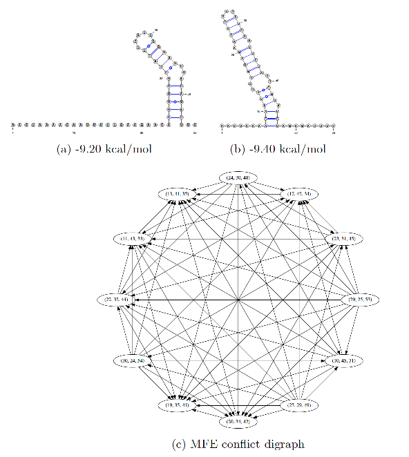
Figure 8: Conflict digraph for the 56 nt spliced leader RNA from L. collosoma with sequence AACUAAAACA AUUUUUGAAG AACAGUUUCU GUACUUCAUU GGUAUGUAGA GACUUC. (a) Metastable structure having free energy of -9.20 kcal/mol. (b) Minimum free energy (MFE) structure having free energy of -9.40 kcal/mol. (c) The RNA conflict digraph for refolding from metastable $s$ to MFE $t$ contains 12 vertices, 61 directed edges and no directed cycles. Minimum free energy (MFE) and metastable structures in (a) and (b) computed by Vienna RNA Package [25]. Secondary structure images generated using VARNA [8].

For the 56 nt L. collosoma spliced leader RNA, whose switching properties were investigated in [18] by stopped-flow rapid-mixing and temperature-jump measurements, the MFE and metastable structures are shown in Figure 8, along with the conflict digraph for $MS_{2}$ folding from the metastable structure to the MFE structure. This RNA has sequence AACUAAAACA AUUUUUGAAG AACAGUUUCU GUACUUCAUU GGUAUGUAGA GACUUC, an MFE structure having -9.40 kcal/mol, and an alternate metastable structure having -9.20 kcal/mol. Figure 8 displays the MFE and metastable structures for L. collosoma spliced leader RNA, along with the conflict digraph for $MS_{2}$ folding from the metastable to the MFE structure.

For L. collosoma spliced leader RNA, if we let $s$ denote the metastable structure and $t$ denote the MFE structure, then there are seven equivalence classes: $X_{1}=\{10,45,31,23\}$ of type 4; $X_{2}=\{11,43,33\}$ of type 3; $X_{3}=\{12,42,34,20\}$ of type 4, $X_{4}=\{13,41,35,19\}$ of type 4, $X_{5}=\{22,32,44\}$ of type 3, $X_{6}=\{24,54,30,48\}$ of type 1, and $X_{7}=\{25,53,29,49\}$ of type 1. As in the case with the 25 nt bistable switch, the equivalence classes for the situation where $s$ and $t$ are interchanged are identical, although type 1 paths become type 4 paths (and vice versa), and type 2 paths become type 3 paths (and vice versa). Output from our (optimal) IP algorithm is as follows.

AACUAAAACAAUUUUUGAAGAACAGUUUCUGUACUUCAUUGGUAUGUAGAGACUUC

12345678901234567890123456789012345678901234567890123456

Number of Nodes: 12

Number of edges: 71

Number of cycles: 5

s: .......................((((((((((((.....)))))..))))))).. -9.20 kcal/mol

t: .......((((((..(((((.((((...)))).)))))..))).)))......... -9.40 kcal/mol

0. .......................((((((((((((.....)))))..))))))).. metastable $s$

1. .......................((.(((((((((.....)))))..)))).)).. remove (26,52)

2. .......................((..((((((((.....)))))..)))..)).. remove (27,51)

3. .......................((...(((((((.....)))))..))...)).. remove (28,50)

4. .......................((....((((((.....)))))..)....)).. remove (29,49)

5. .......................((.....(((((.....))))).......)).. remove (30,48)

6. .......................((...).(((((.....)))))........).. (25,53) -> (25,29)

7. .......................((...))(((((.....)))))........... (24,54) -> (24,30)

8. .........(.............((...)).((((.....)))))........... (31,45) -> (10,45)

9. .........(...........(.((...)).)(((.....))).)........... (32,44) -> (22,32)

10. .........((..........(.((...)).).((.....))).)........... (33,43) -> (11,43)

11. .........(((.........(.((...)).)..(.....))).)........... (34,42) -> (12,42)

12. .........(((......(..(.((...)).)..)......)).)........... (35,41) -> (19,35)

13. .......(.(((......(..(.((...)).)..)......)).).)......... add (8,47)

14. .......(((((......(..(.((...)).)..)......)).)))......... add (9,46)

15. .......(((((...(..(..(.((...)).)..)..)...)).)))......... add (16,38)

16. .......(((((...((.(..(.((...)).)..).))...)).)))......... add (17,37)

17. .......(((((...((((..(.((...)).)..))))...)).)))......... add (18,36)

18. .......(((((...(((((.(.((...)).).)))))...)).)))......... add (20,34)

19 .......(((((...(((((.((((...)))).)))))...)).)))......... add (23,31)

20. .......((((((..(((((.((((...)))).)))))..))).)))......... add (13,41)

Number of base pair removals: 5

Number of base pair additions: 8

Number of base pair shifts: 7

MS2 Distance: 20

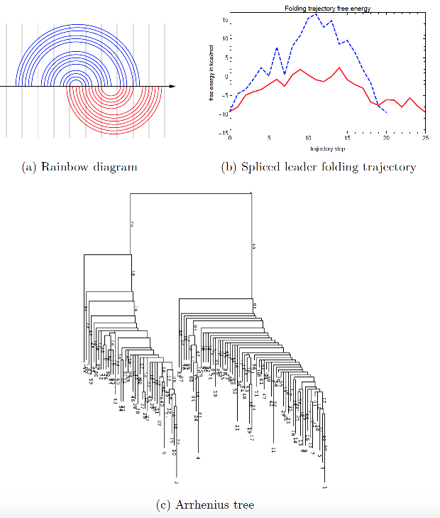
Figure 9: (a) Rainbow diagram for spliced leader RNA from L. collosoma, in which the base pairs for the initial structure $s$ (Figure 8a) are shown below the line in red, while those for the target structure $t$ (Figure 8b) are shown above the line in blue. (b) Free energies of structures in the shortest $MS_{2}$ folding trajectory for spliced leader are shown by the dotted blue line, while those for the energy-optimal $MS_{2}$ folding trajectory are shown in the solid red line. Algorithm 14 was used to compute the shortest $MS_{2}$ trajectory, while the programs RNAsubopt [46] and barriers [14] were used to compute the energy-optimal folding trajectory.

Figure 8a depicts the initial structure $s$, and Figure 8b depicts the target minimum free energy structure $t$ for spliced leader RNA from L. collosoma. The conflict digraph for the refolding from $s$ to $t$ is shown in Figure 8c. Figure 9a displays the rainbow diagram for spliced leader RNA from L. collosoma, in which the base pairs for the initial structure $s$ (Figure 8a) are shown below the line in red, while those for the target structure $t$ (Figure 8b) are shown above the line in blue. Figure 9c displays the Arrhenius tree, where leaf index 2 represents the initial metastable structure $s$ with free energy -9.20 kcal/mol as shown in Figure 8a, while leaf index 1 represents the target MFE structure $t$ with free energy -9.40 kcal/mol as shown in Figure 8b. In Figure 9b, the dotted blue line depicts the free energies of structures in the shortest $MS_{2}$ folding trajectory for spliced leader, as computed by Algorithm 14, while the solid red line depicts the free energies of the energy-optimal folding trajectory as computed by the programs RNAsubopt [46] and barriers [14].

3.2.4 xpt riboswitch from B. subtilis

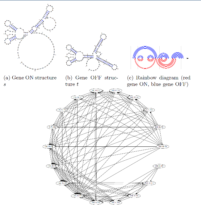
Figure 10: Gene ON and gene OFF structures and the RNA conflict digraph for the 156 nt xanthine phosphoribosyltransferase (xpt) riboswitch from B. subtilis – structures consistent with in-line probing data taken from Figure 1A of [38]. (a) Gene ON structure (default) in absence of free guanine, having (computed) free energy of -33.11 kcal/mol. (b) Gene OFF structure when guanine binds cytidine in position 66, having (computed) free energy of -56.20 kcal/mol (guanine not shown). (c) Rainbow diagram with red gene ON structure below line and blue gene OFF structure above line. Rainbow diagrams allow one to determine by visual inspection when base pairs touch or cross. (d) Conflict digraph $G=(V,E)$, containing 18 vertices, 113 directed edges, and 1806 directed cycles. Minimum free energy (MFE) and metastable structures in (a) and (b) computed by Vienna RNA Package [25]. Free energy computations using Turner energy model [41] computed with Vienna RNA Package [25]. Secondary structure images generated using VARNA [8].

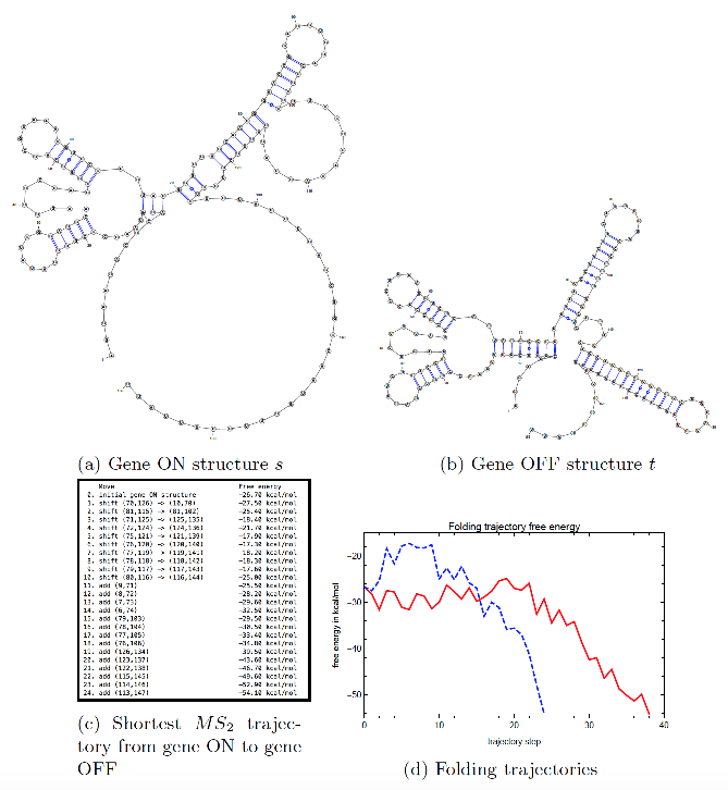
Figure 11: (a) Initial gene ON structure (default) in absence of free guanine (enlarged image). (b) Target gene OFF structure when guanine binds cytidine in position 66 (enlarged image). (c) Shortest $MS_{2}$ folding trajectory from the gene ON structure $s$ to the gene OFF structure $t$ for the 156 nt xpt riboswitch from B. subtilis, described in the caption to Figure 10. Note the initial elongation of the P1 helix by the first shift, followed by the stepwise removal of the anti-terminator and construction of the terminator loops by shift 2-10, followed by base pair additions to lengthen the terminator loop. Although (a,b) are duplicated from the previous figure, this is necessary to follow the sequence of moves in the $MS_{2}$ trajectory. Secondary structure images generated using VARNA [8]. (d) Free energies of structures in the shortest $MS_{2}$ folding trajectory for xpt are shown by the dotted blue line, while those for the an energy near-optimal $MS_{1}$ folding trajectory are shown in the solid red line. Algorithm 14 was used to compute the shortest $MS_{2}$ trajectory, while the program RNAtabuPath [10] was used to compute the energy near-optimal $MS_{1}$ folding trajectory. The size of the 156 nt xpt riboswitch and the fact that the program RNAsubopt would need to generate all secndary structures within 30 kcal/mol of the minimum free energy -54.1 kcal/mol preclude any possibility that the optimal $MS_{2}$ trajectory can be computed by application of the program barriers [14].

In this section, we describe the shortest $MS_{2}$ folding trajectory from the initial gene ON structure $s$ to the target gene OFF structure $t$ for the 156 nt xanthine phosphoribosyltransferase (xpt) riboswitch from B. subtilis, where the sequence and secondary structures are taken from Figure 1A of [38]. The gene ON [resp. OFF] structures for the 156 nt xpt RNA sequence AGGAACACUC AUAUAAUCGC GUGGAUAUGG CACGCAAGUU UCUACCGGGC ACCGUAAAUG UCCGACUAUG GGUGAGCAAU GGAACCGCAC GUGUACGGUU UUUUGUGAUA UCAGCAUUGC UUGCUCUUUA UUUGAGCGGG CAAUGCUUUU UUUAUU are displayed in Figure 10a [resp. 10b], while Figure 10c shows the rainbow diagram, where lower red arcs [resp. upper blue arcs] indicate the base pairs of the initial gene ON [resp. target gene OFF] structure. The default structure for the xpt riboswitch in B. subtilis is the gene ON structure; however, the binding of a guanine nucleoside ligand to cytidine in position 66 triggers a conformational change to the gene OFF structure. Figure 10d depicts the conflict digraph $G=(V,E)$ containing 18 vertices, 113 directed edges, and 1806 directed cycles, which is used to compute the shortest $MS_{2}$ folding trajectory from the gene ON to the gene OFF structure. Figures 11a and 11b show an enlargement of the initial gene ON structure $s$ and target gene OFF structure $t$, which allows us to follow the moves in a shortest $MS_{2}$ trajectory that is displayed in Figure 11c.

4 An algorithm for near-optimal $MS_{2}$ distance

Since the exact IP Algorithm 14 could not compute the shortest $MS_{2}$ folding trajectories between the minimum free energy (MFE) structure and Zuker suboptimal structures for some Rfam sequences of even modest size ($\approx 100$ nt), we designed a near-optimal IP algorithm (presented in this section), and a greedy algorithm (presented in Section D of the Appendix). The exact branch-and-bound algorithm from Appendix C was used to debug and cross-check all algorithms.

The run time complexity of both the exact IP Algorithm 14 and the greedy algorithm is due to the possibly exponentially large set of directed simple cycles in the RNA conflict digraph. By designing a 2-step process, in which the feedback arc set (FAS) problem is first solved for a coarse-grained digraph defined below, and subsequently the feedback vertex set (FVS) problem is solved for each equivalence class, we obtain a much faster algorithm to compute a near-optimal $MS_{2}$ folding trajectory between secondary structures $s$ and $t$ for the RNA sequence $\{a_{1},\ldots,a_{n}\}$. In the first step, we use IP to solve the feedback arc set (FAS) problem for a particular coarse-grained digraph defined below, whose vertices are the equivalence classes as defined in Definition 7. The number of cycles for this coarse-grained digraph is quite manageable, even for large RNAs, hence the FAS can be efficiently solved. After removal of an arc from each directed cycle, topological sorting is applied to determine a total ordering according to which each individual equivalence class is processed. In the second step, Algorithm 14 is applied to each equivalence class in topologically sorted order, whereby the feedback vertex set (FVS) problem is solved for the equivalence class under consideration. In the remainder of this section, we fill in the details for this overview, and then present pseudocode for the near-optimal Algorithm 15.

Given secondary structures $s$ and $t$ for the RNA sequence $\{a_{1},\ldots,a_{n}\}$, we partition the set $[1,n]$ into disjoint sets $A,B,C,D$ as in Section 2 by following equations (5), (6), (7), (8). The union $A\cup B$ is subsequently partitioned into the equivalence classes $X_{1},\ldots,X_{m}$, defined in Definition 7. Define the coarse-grain, conflict digraph $G=(V,E)$, whose vertices are the indices of equivalence classes $X_{1},\ldots,X_{m}$, and whose directed edges $i\rightarrow j$ are defined if there exists a base pair $(x,y)\in s$, $x,y\in X_{i}$ which crosses a base pair $(u,v)\in t$, $u,v\in X_{j}$. Although there may be many such base pairs $(x,y)\in s$ and $(u,v)\in t$, there is only one edge between $i$ and $j$; i.e. $G$ is a directed graph, not a directed multi-graph. If $i\rightarrow j$ is an edge, then we define $N_{i,j}$ to be the set of all base pairs $(u,v)\in s$, $u,v\in X_{i}$ that cross some base pair $(u,v)\in t$, $u,v\in X_{j}$, and let $n_{i,j}$ the number of base pairs in $N_{i,j}$. Formally, given equivalence classes $X_{1},\ldots,X_{m}$, the coarse-grain, conflict digraph $G=(V,E)$ is defined by

$$V =\{1,\ldots,m\}$$ (20)

$$E =\Big{\{}i\rightarrow j:\exists(x,y)\in s\exists(u,v)\in t\big{[}x,y\in X_{i}\land u,v\in X_{j}\big{]}\Big{\}}$$ (21)

A directed edge from $i$ to $j$ may be denoted either by $i\rightarrow j\in E$ or by $(i,j)\in E$. For each edge $i\rightarrow j$, we formally define $N_{i,j}$ and $n_{i,j}$ by the following.

$$N_{i,j} =\Big{\{}(x,y)\in s:x,y\in X_{i}\land\exists(u,v)\in t\big{[}u,v\in X_{j}\land\mbox{ $(x,y)$ crosses $(u,v)$ }\big{]}\Big{\}}$$ (22)

$$n_{i,j} =\Big{|}N_{i,j}\Big{|}$$ (23)

We now solve the feedback arc set (FAS) problem, rather than the feedback vertex set (FVS) problem, for digraph $G$, by applying an IP solver to solve the following optimization problem:

1. maximize $\sum_{(i,j)\in E}n_{i,j}\cdot x_{i,j}$ subject to constraint ($\sharp$):

($\sharp$) $\sum\limits_{\stackrel{{\scriptstyle(i,j)\in E}}{{i,j\in C}}}x_{i,j}<|C|$

for every directed cycle $C=\left(i_{1},i_{2},i_{3},\ldots,i_{k-1},i_{k}\right)$

This IP problem can be quickly solved, since there is usually only a modest number of directed cycles for the coarse-grained digraph. For each directed edge or arc $i\rightarrow j$ that is to be removed from a directed cycle, we remove all base pair $(x,y)\in$ from structure $s$ that cross some base pair $(u,v)\in t$ for which $u,v\in X_{j}$. Removal of certain base pairs from $s$ can disconnect some previous equivalence classes into two or more connected components, hence equivalence classes $X^{\prime}_{1},\ldots,X^{\prime}_{m^{\prime}}$ must be recomputed for the updated structure $s$ and (unchanged) structure $t$. The conflict, digraph $G^{\prime}=(V^{\prime},E^{\prime})$ is then defined by equations (20) and (21) for (updated) $s$ and (unchanged) $t$. Since $G^{\prime}$ is now acyclic, it can be topologically sorted, which determines an ordering $\sigma(1),\ldots,\sigma(m^{\prime})$ for processing equivalence classes $X^{\prime}_{1},\ldots,X^{\prime}_{m^{\prime}}$. To process an equivalence class $X^{\prime}$, we restrict the exact Algorithm 14 to each equivalence class. Indeed, to process equivalence class $X^{\prime}$, we define a (local) conflict digraph $G(X^{\prime})=(V(X^{\prime}),E(X^{\prime}))$ defined as follows.

$$V(X^{\prime}) =\{(x,y,z):x,y,z\in X^{\prime}\land\{x,y\}\in t\land\{y,z\}\in s$$ (24)

$$E(X^{\prime}) =\{(x,y,z)\rightarrow(u,v,w):(x,y,z)\in V(X^{\prime})\land(u,v,w)\in V(X^{\prime})\land$$ (25)

$$\quad\mbox{ $\{x,y\}$ touches or crosses $\{v,w\}$ }\}$$

Algorithm 15 (Near-optimal $MS_{2}$ distance from $s$ to $t$).

Input: Secondary structures $s,t$ for RNA sequence $a_{1},\ldots,a_{n}$ Output: $s=s_{0},s_{1},\ldots,s_{m}=t$, where $s_{0},\ldots,s_{m}$ are secondary structures, $m$ is a near-optimal value for which $s_{i}$ is obtained from $s_{i-1}$ by a single base pair addition, removal or shift for each $i=1,\ldots,m$.

First, initialize the variable numMoves to $0$, and the list moveSequence to the empty list [  ]. Define $BP_{1}=\{(x,y):(x,y)\in t,(t-s)[x]=0,(t-s)[y]=0\}$; i.e. $BP_{1}$ consists of those base pairs in $s$ which are not touched by any base pair in $t$. Define $BP_{2}=\{(x,y):(x,y)\in t,(s-t)[x]=0,(s-t)[y]=0\}$; i.e. $BP_{2}$ consists of those base pairs in $t$ which are not touched by any base pair in $s$.

//remove base pairs from $s$ that are untouched by $t$

1. for $(x,y)\in BP_{1}$

2. $s=s-\{(x,y)\}$

3. numMoves = numMoves + 1

//define equivalence classes on updated $s,t$

4. $[1,n]=A\cup B\cup C\cup D$

5. determine equivalence classes $X_{1},\ldots,X_{m}$ with union $A\cup B$

//define conflict digraph $G=(V,E)$ on collection of equivalence classes

6. define $V=\{1,\ldots,m\}$

7. define $E=\{(i,j):1\leq i,j\leq m\}$ by equation (21)

8. define coarse-grain, conflict digraph $G=(V,E)$

//IP solution of feedback arc set problem (not feedback vertex set problem)

9. maximize $\sum_{(i,j)\in E}n_{i,j}\cdot x_{i,j}$ subject to constraint ($\sharp$):

//remove arc from each simple cycle where$n_{i,j}$ defined in equation (23)

($\sharp$) $\sum\limits_{\stackrel{{\scriptstyle(i,j)\in E}}{{i\rightarrow j\in C}}}x_{i,j}<|C|$

for every directed cycle $C=\left(i_{1},i_{2},\ldots,i_{k-1},i_{k}\right)$

10. $\widetilde{E}=\{(i,j):x_{i,j}=0\}$ //$\widetilde{E}$ is set of edges that must be removed

//process the IP solution $\widetilde{E}$

11. for $(i,j)\in\widetilde{E}$

12. for $(x,y)\in N_{i,j}$ //$N_{i,j}$ defined in Definition 22

13. $s=s-\{(x,y)\}$ //remove base pair from $s$ belonging to feedback arc

14. numMoves = numMoves + 1

//determine equivalence classes ${X^{\prime}}_{1},\ldots,{X^{\prime}}_{m^{\prime}}$ for updated $s$ and (unchanged) $t$

15. $[1,n]=A^{\prime}\cup B^{\prime}\cup C^{\prime}\cup D^{\prime}$

16. define ${X^{\prime}}_{1},\ldots,{X^{\prime}}_{m^{\prime}}$ whose union is $(A^{\prime}\cup B^{\prime})$

17. define $V^{\prime}=\{1,\ldots,m^{\prime}\}$

18. define $E^{\prime}=\{(i,j):1\leq i,j\leq m^{\prime}\}$ by equation (21)

19. define $G^{\prime}=(V^{\prime},E^{\prime})$ //note that $G^{\prime}$ is an acyclic multigraph

20. let $\sigma\in S_{m^{\prime}}$ be a topological sort of $V^{\prime}$//$S_{m^{\prime}}$ denotes set of all permutations on $[1,m^{\prime}]$

//process shifts in $X_{\sigma(i)}$ in topological order by adapting part of Algorithm 14

21. for $i=1$ to $m^{\prime}$

22. define $V(X_{\sigma(i)})$ by equation (24)

23. define $E(X_{\sigma(i)})$ by equation (25)

24. define $G(X_{\sigma(i)})=(V(X_{\sigma(i)}),E(X_{\sigma(i)}))$

//IP solution of minimum feedback vertex set problem

25. maximize $\sum_{v\in V(X_{\sigma(i)})}x_{v}$ where $x_{v}\in\{0,1\}$, subject to constraints (${\dagger}_{i}$) and (${\ddagger}_{i}$)

//first constraint removes vertex from each simple cycle of $G(X_{\sigma(i)})$

(${\dagger}_{i}$) $\sum\limits_{v\in C}x_{v}<|C|$ for each simple directed cycle $C$ of $G(X_{\sigma(i)})$

//ensure shift moves cannot be applied if they share same base pair from $s$ or $t$

(${\ddagger}_{i}$) $x_{v}+x_{v^{\prime}}\leq 1$, for distinct vertices $v=(x,y,z),v^{\prime}=(x^{\prime},y^{\prime},z^{\prime})$ with $|\{x,y,z\}\cap\{x^{\prime},y^{\prime},z^{\prime}\}|=2$

//define the induced, acyclic digraph $\overline{G}(X_{\sigma(i)})$

26. $\overline{V}(X_{\sigma(i)})=\{v\in V(X_{\sigma(i)}):x_{v}=1\}$

27. $\overline{E}(X_{\sigma(i)})=\{(v,v^{\prime}):v,v^{\prime}\in\overline{V}\land(v,v^{\prime})\in E(X_{\sigma(i)})\}$

28. let $\overline{G}(X_{\sigma(i)})=(\overline{V}(X_{\sigma(i)}),\overline{E}(X_{\sigma(i)}))$

//handle special, closed 2-cycles

29. for each closed 2-cycle $[x]=\{a_{1},a_{2},a_{3},a_{4}\}$ as depicted in Figure 5

30. if $[x]$ is of type A as depicted in Figure 5a

31. remove base pair from $s$ by equation (18)

32. if $[x]$ is of type B as depicted in Figure 5b

33. remove base pair from $s$ by equation (19)

//remove base pairs from $s$ that are not involved in a shift move

34. $\overline{V}(X_{\sigma(i)}).s=\{(x,y):\exists v\in\overline{V}(X_{\sigma(i)})(v.s=(x,y))\}$

35. for $(x,y)\in s-t$

36. if $(x,y)\not\in\overline{V}(X_{\sigma(i)}).s$

37. remove $(x,y)$ from $s$; numMoves = numMoves+1

//topological sort of IP solution $\overline{V}(X_{\sigma(i)})$

38. topological sort of $\overline{G}(X_{\sigma(i)})$ using DFS to obtain total ordering $\prec$ on $\overline{V}(X_{\sigma(i)})$

38. for $v=(x,y,z)\in\overline{V}$ in topologically sorted order $\prec$

//check if shift would create a base triple, as in type 1,5 paths from Figure 3

40. if $s[x]=1$ //i.e. $\{u,x\}\in s$ for some $u\in[1,n]$

41. remove $\{u,x\}$ from $s$; numMoves = numMoves+1

42. shift $\{y,z\}$ to $\{x,y\}$ in $s$; numMoves = numMoves+1

//remove any remaining base pairs from $s$ that have not been shifted

43. for $(y,z)\in s-t$ which satisfy $y,z\in X_{\sigma(i)}$

44. if $(x,y,z)\in V(X_{\sigma(i)})$ where $x=t[y]$

45. shift base pair $\{y,z\}\in s$ to $\{x,y\}\in t$; numMoves = numMoves+1

46. else //$\{y,z\}$ is a remaining base pair of $s$ but cannot be applied in a shift

47. remove $(x,y)$ from $s$; numMoves = numMoves+1

//add remaining base pairs from $t$ to $s$

48. for $(x,y)\in t-s$

49. $s=s\cup\{(x,y)\}$

50. numMoves = numMoves + 1

51. return moveSequence, numMoves

5 Benchmarking results

5.1 Random sequences

Given a random RNA sequence ${\bf a}=a_{1},\ldots a_{n}$ of length $n$, we generate a list $L$ of all possible base pairs, then choose with uniform probability a base pairs $(x,y)$ from $L$, add $(x,y)$ to the secondary structure $s$ being constructed, then remove all base pairs $(x^{\prime},y^{\prime})$ from $L$ that either touch or cross $(x,y)$, and repeat these last three steps until we have constructed a secondary structure having the desired number ($n/5$) of base pairs. If the list $L$ is empty before completion of the construction of secondary structure $s$, then reject $s$ and start over. The following pseudocode describes how we generated the benchmarking data set, where for each sequence length $n=10,15,20,\cdots,150$ nt, twenty-five random RNA sequences were generated of length $n$, with probability of $1/4$ for each nucleotide, in which twenty secondary structures $s,t$ were uniformly randomly generated for each sequence so that 40% of the nucleotides are base-paired.

1. for $n$ = 10 to 150 with step size 10

2. for numSeq = 1 to 25

3. generate random RNA sequence ${\bf a}=a_{1},\ldots,a_{n}$ of length $n$

4. generate $20$ random secondary structures of ${\bf a}$

5. for all ${20\choose 2}=190$ pairs of structures $s,t$ of ${\bf a}$

6. compute optimal and near-optimal $MS_{2}$ folding trajectories from $s$ to $t$

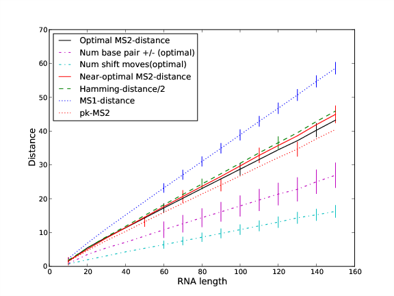
Figure 12: Benchmarking statistics for optimal and near-optimal algorithm to compute minimum length $MS_{2}$ folding trajectories between random secondary structures $s,t$ of random RNA sequences of variable lengths. For each sequence length $n=10,15,20,\cdots,150$ nt, twenty-five random RNA sequences were generated of length $n$, with probability of $1/4$ for each nucleotide. For each RNA sequence, twenty secondary structures $s,t$ were uniformly randomly generated so that 40% of the nucleotides are base-paired. Thus the number of computations per sequence length is thus $25\cdot 190=4750$, so the size of the benchmarking set is $15\cdot 4750=71,250$. Using this dataset, the average $MS_{2}$ distance was computed for both the exact IP Algorithm 14 and the near-optimal Algorithm 15. In addition to $MS_{2}$ distance computed by the exact IP and the near-optimal algorithm, the figure displays $pk-MS_{2}$ distance (allowing pseudoknots in intermediate structures) as computed by Algorithm 9, the $MS_{1}$ distance (also known as base pair distance), Hamming distance over 2, and provides a breakdown of the $MS_{1}$ distance in terms of the number of base pair addition/removal moves “num base pair +/- (optimal)” and the shift moves “num shift moves (optimal)”.

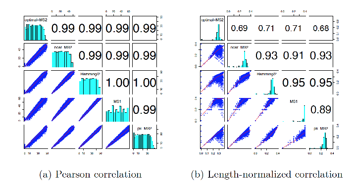
Figure 13: Pairwise correlations for optimal $MS_{2}$ distance, $pk-MS_{2}$ distance, near-optimal $MS_{2}$ distance, Hamming distance divided by $2$, and $MS_{1}$ distance (also called base pair distance). For each two measures, scatter plots were created for the $71,250$ many data points from the benchmarking set described in Figure 12. Pearson correlation and normalized Pearson correlation values computed, where by normalized, we mean that for each of the $71,250$ data points, we consider the length-normalized distance (distance divided by sequence length). These correlations are statistically significant – each Pearson correlation values has a $p$-value less than $10^{-8}$.

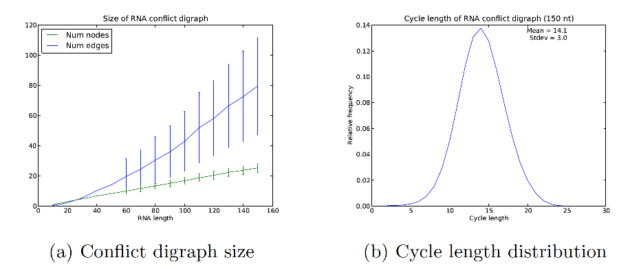
Figure 15: (Left) Average size of vertex sets $V$ and of directed edge sets $E$ for RNA conflict digraphs $G=(V,E)$ for the data set of described in Figure 12. Error bars represent $\pm 1$ standard deviation. Clearly the size of a conflict digraph grows linearly in the length $n$ of random RNAs ${\bf a}=a_{1},\ldots,a_{n}$, given random secondary structures $s,t$ having $n/5$ base pairs. (Right) Cycle length distribution for random RNAs ${\bf a}=a_{1},\ldots,a_{n}$ of length $n=150$, with randomly chosen secondary structures $s,t$ having $n/5$ base pairs, using data extracted from the data set described in Figure 12. For values of $n=50,\ldots,150$, the cycle length distribution appears approximately normal, although this is not the case for $n\leq 40$ (data not shown).

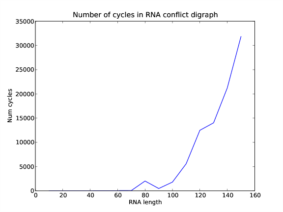
Figure 16: Average number of directed cycles as a function of sequence length for the data set described in Figure 12. For each random RNA sequence ${\bf a}=a_{1},\ldots,a_{n}$ of length $n$, and for each pair of random secondary structures $s,t$ of ${\bf a}$ having $n/5$ base pairs, we computed the total number of directed cycles in the conflict digraph $G({\bf a},s,t)$. The figure suggests that starting at a threshold sequence length $n$, there is an exponential growth in the number of directed cycles in the conflict digraph of random sequences of length $n$.

The number of computations per sequence length is thus $25\cdot 190=4750$, so the size of the benchmarking set is $15\cdot 4750=71,250$. This benchmarking set is used in Figures 12 – 16. Figure 12 compares various distance measures discussed in this paper: $MS_{2}$ distance computed by the optimal IP Algorithm 14, approximate $MS_{2}$ distance computed by the near-optimal Algorithm 15, $pk-MS_{2}$ distance that allows pseudoknotted intermediate structures, $MS_{1}$ distance, and Hamming distance divided by 2. Additionally, this figure distinguishes the number of base pair additions/removals and shifts in the $MS_{2}$ distance.

Figure 13a shows the scatter plots and Pearson correlation coefficients all pairs of the distance measures: $MS_{2}$ distance, near-optimal $MS_{2}$ distance, $pk-MS_{2}$ distance, Hamming distance divided by $2$, $MS_{1}$ distance. In contrast to Figure 13, the second panel Figure 13b shows the length-normalized values. It is unclear why $MS_{2}$ distance has a slightly higher length-normalized correlation with both Hamming distance divided by 2 and $MS_{1}$ distance, than that with approximate $MS_{2}$ distance, as computed by Algorithm 15 – despite the fact that the latter algorithm approximates $MS_{2}$ distance much better than either Hamming distance divided by 2 or $MS_{1}$ distance. Figure 14 shows that run-time of Algorithms 14 and 15, where the former is broken down into time to generate the set of directed cycles and the time for the IP solver. Note that there is a 10-fold speed-up in Algorithm 14 from this paper, compared with a precursor of this algorithm that appeared in the proceedings of the Workshop in Bioinformatics (WABI 2017). Since Algorithm 15 applies Algorithm 14 to each equivalence class, there is a corresponding, but less striking speed-up in the near-optimal algorithm. Since run-time depends heavily on the number of directed cycles in the conflict digraphs, Figure 15a shows the size of vertex and edge sets of the conflict digraphs for the benchmarking data, and Figure 15b depicts the cycle length distribution for benchmarking data of length 150; for different lengths, there are similar distributions (data not shown). Finally, Figure 15c showns the (presumably) exponential increase in the number of directed cycles, as a function of sequence length. Since Algorithm 15 does not compute the collection of all directed cycles (but only those for each equivalence class), the run time of Algorithm 15 appears to be linear in sequence length, compared to the (presumably) exponential run time of Algorithm 14.

5.2 Rfam sequences

In this section, we use data from the Rfam 12.0 database [28] for analogous computations as those from the previous benchmarking section. For each Rfam family having average sequence length less than 100 nt, one sequence is randomly selected, provided that the base pair distance between its MFE structure and its Rfam consensus structure is a minimum. For each such sequence ${\bf a}$, the target structure $t$ was taken to be the secondary structure having minimum free energy among all structures of ${\bf a}$ that are compatible with the Rfam consensus structure, as computed by RNAfold -C [25] constrained with the consensus structure of ${\bf a}$. The corresponding initial structure $s$ for sequence ${\bf a}$ was selected from a Zuker-suboptimal structure, obtained by RNAsubopt -z [25], with the property that $|d_{\mbox{\small BP}}(s,t)-d_{\mbox{\small H}}(s,t)|<0.2\cdot d_{\mbox{\small BP}}(s,t)$. Since we know from Figure 14 that run time of the optimal IP Algorithm 14 depends on the number of cycles in the corresponding RNA conflict digraph, the last criterion is likely to result in a less than astronomical number of cycles. The resulting dataset consisted of 1333 sequences, some of whose lengths exceed 100 nt. Nevertheless, the number of cycles in the RNA constraint digraph of 22 of the 1333 sequences exceeded 50 million (an upper bound set for our program), so all figures described in this section are based on 1311 sequences from Rfam.

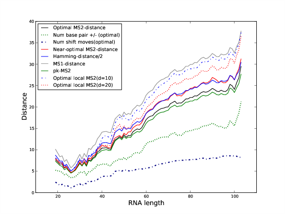
Figure 17: Moving averages of distance measures graphed as a function of sequence length for the $1311$ many sequences extracted from Rfam 12.0 (see text). Distance measures included optimal $MS_{2}$-distance computed by the exact IP (optimal) algorithm 14 (where the number of base pair additions ($+$) or removals ($-$) is indicated, along with the number of shifts),, near-optimal $MS_{2}$-distance computed by near-optimal algorithm 15, Hamming distance divided by $2$, $MS_{1}$ distance aka base pair distance, pseudoknotted $MS_{2}$ distance (pk-$MS_{2}$) computed from Lemma 8, optimal local $MS_{2}$ with parameter $d=10$, and optimal local $MS_{2}$ with parameter $d=20$. The latter values were computed by a variant of the exact IP algorithm 14 where shift moves were restricted to be local with parameter $d$, whereby base pair shifts of the form $(x,y)\rightarrow(x,z)$ or $(y,x)\rightarrow(z,x)$ were allowed only when $|y-z|\leq d$. All moving averages were computed over symmetric windows of size 9, i.e. $[i-4,i+4]$. From smallest to largest value, the measures are: number of shifts in optimal $MS_{2}$ trajectory $<$ number of base pair additions or deletions ($+/-$) in optimal $MS_{2}$ trajectory $<$ pk-$MS_{2}$ $<$ $MS_{2}$ distance $<$ Hamming distance over $2$ $\approx$ near-optimal $MS_{2}$ $<$ $MS_{2}$ with locality parameter $d=20$ $<$ $MS_{2}$ with locality parameter $d=10$ $<$ $MS_{1}$.

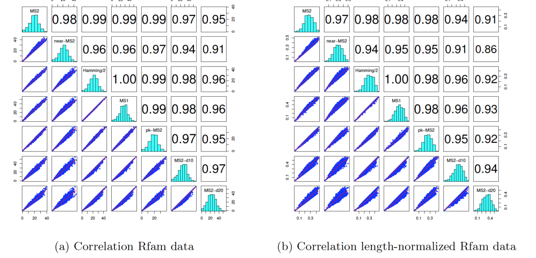
Figure 18: Pairwise correlations using Rfam benchmarking data (see text) for optimal $MS_{2}$ distance, $pk-MS_{2}$ distance, near-optimal $MS_{2}$ distance, Hamming distance divided by $2$, and $MS_{1}$ distance (also called base pair distance). For each two measures, scatter plots were created for the $1311$ many data points. Pearson correlation and normalized Pearson correlation values computed, where by normalized, we mean that for each of the $1311$ data points, we consider the length-normalized distance (distance divided by sequence length). These correlations are statistically significant – each Pearson correlation values has a $p$-value less than $2.2\cdot 10^{-16}$.

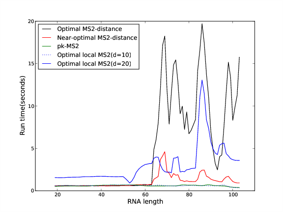
Figure 19: Moving averages of run time as a function of sequence length for the $1311$ sequences extracted from Rfam 12.0 (see text). Distance measures considered are the exact $MS_{2}$ distance computed by the optimal IP Algorithm 14, an approximation to the $MS_{2}$ distance computed by the near-optimal IP Algorithm 15, the $pk-MS_{2}$ distance (allowing pseudoknots in intermediate structures) as computed by Algorithm 9, and two variants of exact $MS_{2}$ distance, where shifts are restricted by locality parameter $d=10,20$. These latter values were computed by the exact IP Algorithm 14 modified to allow base pair shifts of the form $(x,y)\rightarrow(x,z)$ or $(y,x)\rightarrow(z,x)$ only when $|y-z|\leq d$.

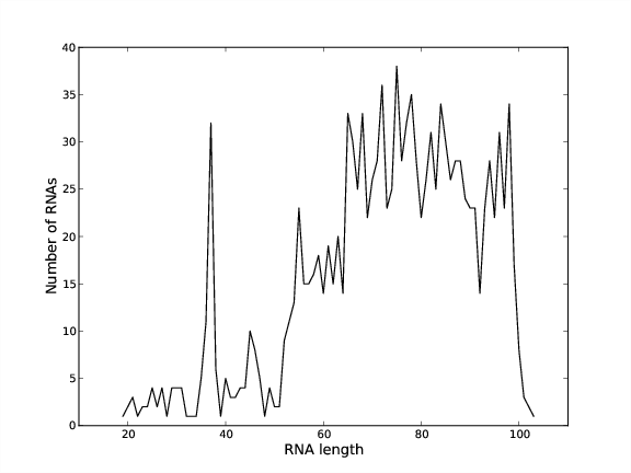
Figure 20: Number of sequences as a function of sequence length for the 1311 sequences extracted from Rfam 12.0 and used in benchmarking tests (see text).

Figure 17 depicts the moving averages in centered windows $[x-2,x+2]$ of the following distance measures for the $1311$ sequences extracted from Rfam 12.0 as described. Distance measures include (1) optimal $MS_{2}$-distance computed by the exact IP (optimal) Algorithm 14 (where the number of base pair additions ($+$) or removals ($-$) is indicated, along with the number of shifts), (2) near-optimal $MS_{2}$-distance computed by near-optimal Algorithm 15, (3) Hamming distance divided by $2$, (4) $MS_{1}$ distance aka base pair distance, (5) pseudoknotted $MS_{2}$ distance (pk-$MS_{2}$) computed from Algorithm 9, (6) optimal local $MS_{2}$ with parameter $d=10$, and (7) optimal local $MS_{2}$ with parameter $d=20$. The latter values were computed by a variant of the exact IP Algorithm 14 with locality parameter $d$, defined to allow base pair shifts of the form $(x,y)\rightarrow(x,z)$ or $(y,x)\rightarrow(z,x)$ only when $|y-z|\leq d$. This data suggests that Hamming distance over $2$ ($d_{\mbox{\small H}}(s,t)/2$) closely approximates the distance computed by near-optimal Algorithm 15, while pk-$MS_{2}$ distance ($d_{\mbox{\small pk-$MS_{2}$}}(s,t)$) is a better approximation to $MS_{2}$ distance than is Hamming distance over $2$. Figure 18 presents scatter plots and Pearson correlation values when comparing various distance measures using the Rfam data. Figure 18a [resp. Figure 18b] presents Pearson correlation [resp. normalized Pearson correlation] values computed, where by normalized, we mean that for each of the $1311$ extracted Rfam sequences ${\bf a}$ with corresponding initial structure $s$ and target structure $t$, the length-normalized distance measures $d(s,t)/|{\bf a}|$ are correlated. Figure 19 depicts the moving average run times as a function of sequence length, where for given value $x$ the run times are averaged for sequences having length in $[x-2,x+2]$. Finally, Figure 20 depicts the number of sequences of various lengths used in the Rfam benchmarking set of 1311 sequences.

6 Conclusion

In this paper, we have introduced the first optimal and near-optimal algorithms to compute the shortest RNA secondary structure folding trajectories in which each intermediate structure is obtained from its predecessor by the addition, removal or shift of a base pair; i.e. the shortest $MS_{2}$ trajectories. Since helix zippering and defect diffusion employ shift moves, one might argue that it is better to include shift moves when physical modeling RNA folding, and indeed the RNA folding kinetics simulation program Kinfold [13] uses the $MS_{2}$ move set by default. Using the novel notion of RNA conflict directed graph, we describe an optimal and near-optimal algorithm to compute the shortest $MS_{2}$ folding trajectory. Such trajectories pass through substantially higher energy barriers than trajectories produced by Kinfold, which uses Gillespie’s algorithm [17] (a version of event-driven Monte Carlo simulation) to generate physically realistic $MS_{2}$ folding trajectories. We have shown in Theorem 2 that it is NP-hard to compute the $MS_{2}$ folding trajectory having minimum energy barrier, and have presented anecdotal evidence that suggests that it may also NP-hard to compute the shortest $MS_{2}$ folding trajectory. For this reason, and because of the exponentially increasing number of cycles (see Figure 16) and subsequent time requirements of our optimal IP Algorithm 14, it is unlikely that (exact) $MS_{2}$ distance prove to be of much use in molecular evolution studies such as [3, 42, 15]. Nevertheless, Figures 12 and 17 suggest that either pk-$MS_{2}$ distance and/or near-optimal $MS_{2}$ distance may be a better approximation to (exact) $MS_{2}$ distance than using Hamming distance, as done in [36, 43]. However, given the high correlations between these measures, it is unlikely to make much difference in molecular evolution studies.

Our graph-theoretic formulation involving RNA conflict digraphs raises some interesting mathematical questions partially addressed in this paper; in particular, it would be very interesting to characterize the class of digraphs that can be represented by RNA conflict digraphs, and to determine whether computing the shortest $MS_{2}$ folding trajectory is $NP$-hard. We hope that the results presented in this paper may lead to resolution of these questions.

7 Figures

Figure 2: Defect diffusion [31], where a bulge migrates stepwise to become absorbed in an hairpin loop. The move from structure (a) to structure (b) is possible by the shift $(1,12)\rightarrow(1,13)$, the move from (b) to (c) by shift $(2,11)\rightarrow(2,12)$, etc. Our algorithm properly accounts for such moves with respect to energy models A,B,C. Image taken from [6].

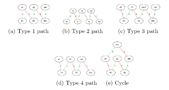
Figure 3: All possible maximal length red-green paths and cycles. Each equivalence class $X$, as defined in Definition 7, can be depicted as a maximal length path or cycle, consisting of those positions $x\in[1,n]$ that are connected by alternating base pairs drawn from secondary structures $s$ (green) and $t$ (red). Each path or cycle $X$ is depicted in a fashion that the leftmost [resp. rightmost position] satisfies the following properties, where $End(s,X)$ [resp. $End(t,X)$] denotes the set of elements of $X$ that are untouched by $t$ [resp. $s$]: for paths of type 1, $|X|$ is even, $|End(s,X)]=2$, $b_{1}=\min(End(s,X))$, $t[a_{m}]=0$; for paths of type 2, $|X|$ is odd, $|End(s,X)]=1=|End(t,X)|$, $b_{0}=\min(End(s,X))$, $s[b_{m}]=0$; for paths of type 3, $|X|$ is odd, $|End(s,X)]=1=|End(t,X)|$, $a_{0}=\min(End(t,X))$, $t[a_{m}]=0$; for paths of type 4, $|X|$ is even, $|End(t,X)]=2$, $a_{1}=\min(End(t,X))$, $s[b_{m}]=0$; for paths of type 5, or cycles, $|X|$ must be even, and $a_{1}=\min(X)$. Note that the appearance of positions in left-to-right order does not necessarily respect integer ordering, so the leftmost position is not necessarily the minimum $\min(X)$, nor is the rightmost position necessarily the maximum $\max(X)$.

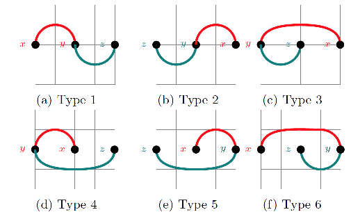
Figure 4: All six possible shift moves, in which a base pairs of $s$ (teal) that touches a base pairs of $t$ (red) is shifted, thus reducing the base pair distance $d_{\mbox{\small BP}}(s,t)$ by $2$. Each such shift move can uniquely be designated by the triple $(x,y,z)$, where $y$ is the pivot position (common position to a base pair in both $s$ and $t$), $x$ is the remaining position in the base pair in $t$, and $z$ is the remaining position in the base pair in $s$.

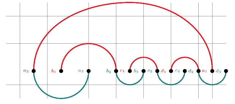
Figure 21: RNA conflict digraph $G=(V,E)$ for secondary structures $t$ and $s$, where $t=\{(a_{2},a_{1}),(b_{1},b_{2}),(c_{1},c_{2}),(d_{1},d_{2})\}$, and $s=\{(a_{2},a_{3}),(b_{2},b_{3}),(c_{2},c_{3}),(d_{2},d_{3})\}$. The triplet nodes of $V=\{v_{a},v_{b},v_{c},v_{d}\}$ are the following: $v_{a}=(a_{1},a_{2},a_{3})$ of type 3, shift $v_{b}=(b_{1},b_{2},b_{3})$ of type 1, shift $v_{c}=(c_{1},c_{2},c_{3})$ of type 1, and shift $v_{d}=(d_{1},d_{2},d_{3})$ of type 1. The edges in $E$ are the following: $v_{a}\rightarrow v_{b}$, $v_{b}\rightarrow v_{c}$, $v_{c}\rightarrow v_{d}$, $v_{d}\rightarrow v_{a}$. The conflict digraph $G=(V,E)$ is order-isomorphic to the digraph $G^{\prime}=(V^{\prime},E^{\prime})$, where $V^{\prime}=\{1,2,3,4\}$ and edges are as follows: $1\rightarrow 2\rightarrow 3\rightarrow 4\rightarrow 1$.

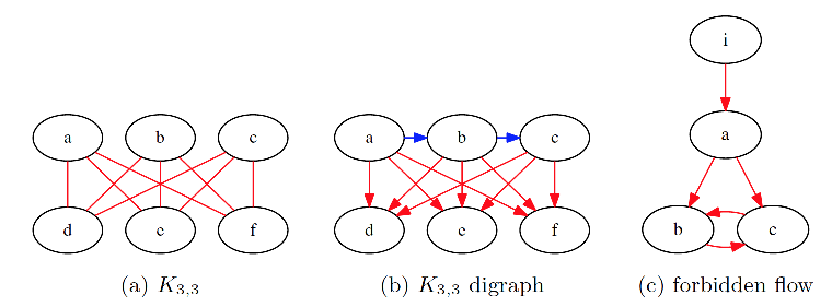
Figure 22: (a) Complete bipartite graph $K_{3,3}$. A finite graph is planar if and only if it does not contain the forbidden graph $K_{3,3}$ or the complete graph $K_{5}$ [24]. (b) Directed graph realized by the RNA conflict digraph in Figure 23. It follows that RNA conflict digraphs are not necessarily planar. (c) Directed graph realized by the RNA conflict digraph in Figure 24. A flow graph is reducible if and only if it does not contain such a forbidden flow graph, where edges between nodes may be replaced by arc-disjoint directed paths [19]. It follows that RNA conflict digraphs are not necessarily reducible flow graphs.

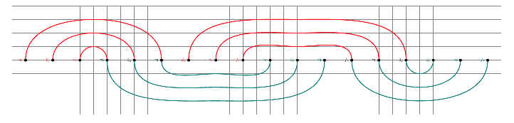
Figure 23: RNA conflict digraph that realizes the digraph $K_{3,3}$ depicted in Figure 22b, whose undirected red edges represent the undirected graph $K_{3,3}$ depicted in Figure 22b. The nonplanar complete, bipartite digraph $K_{3,3}$, with shift moves $c,b,a,d,e,f$, all of type 1, in order from left to right – i.e. order of positions along the $x$-axis is given by: $c_{1},b_{1},a_{1},a_{2},b_{2},c_{2}$, $d_{1},e_{1},f_{1},c_{3},b_{3},a_{3}$, $f_{2},e_{2},d_{2},d_{3},e_{3},f_{3}$. Notice that $a_{s}$ crosses $b_{t}$, $c_{t}$, $d_{t}$, $e_{t}$ and $f_{t}$ so $c\leftarrow a$, $b\leftarrow a$ and $a\rightarrow d$, $a\rightarrow e$, $a\rightarrow f$; $b_{s}$ crosses $c_{t}$, $d_{t}$, $e_{t}$ and $f_{t}$ so $c\leftarrow b$ and $b\rightarrow d$, $b\rightarrow e$, $b\rightarrow f$; $c_{s}$ crosses $d_{t}$, $e_{t}$ and $f_{t}$ so $c\rightarrow d$, $c\rightarrow e$, $c\rightarrow f$.

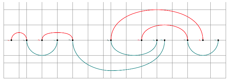
Figure 24: Forbidden flow graph with nodes $i=(i_{1},i_{2},i_{3})$, $a=(a_{1},a_{2},a_{3})$, $b=(b_{1},b_{2},b_{3})$, $c=(c_{1},c_{2},c_{3})$, where nodes $i,a,c$ are of type 1 and node $b$ is of type 3. Notice that $i_{s}$ crosses $a_{t}$ so $i\rightarrow a$; $a_{s}$ crosses $b_{t}$ so $a\rightarrow b$; $a_{s}$ crosses $c_{t}$ so $a\rightarrow c$; $b_{s}$ crosses $c_{t}$ so $b\rightarrow c$; $c_{s}$ crosses $b_{t}$ so $c\leftarrow b$.

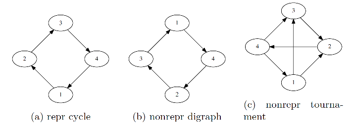
Figure 25: (a) Digraph of an ordered 4-cycle, which is representable by an RNA conflict digraph, as shown in Figure 21. (b) Digraph of an ordered 4-cycle, which is not representable by an RNA conflict digraph. Note that digraph (b) is Eulerian, with the property that the in-degree of each vertex equals its out-degree. (c) Digraph of a tournament on 4 vertices, which is not representable by an RNA conflict digraph. Digraph (a) is isomorphic with digraph (b), thus showing that representability is not preserved under isomorphism. Since it is not difficult to show that all $2^{{3\choose 2}}=8$ tournaments on 3 nodes are representable by RNA conflict digraphs (data not shown), it follows that digraph (c) is a minimum sized non-representable tournament, which we verified by constraint programming. In general there are $2^{{n\choose 2}}$ many tournaments on $n$.

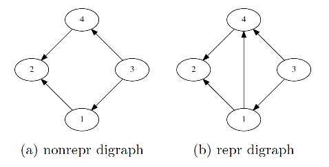
Figure 26: Example of a 4-node digraph in (a) that is not representable by an RNA conflict digraph. However, by adding an edge to digraph (a), we obtain a representable digraph in (b). Note that digraph (a) is neither order-isomorphic to digraph (b), nor is there an order-preserving embedding of digraph (a) into digraph (b).

Appendix A Classification of edges in RNA constraint digraphs

In this section, we describe the collection of all possible directed edges $v\rightarrow v^{\prime}$ in which $v.s$ crosses $v^{\prime}.t$, that can appear in an RNA conflict digraph, classified as forward, backward or 2-cycles and according to each type of vertex (see Figure 4 for the six types of vertices). It is straightforward for the reader to imaging additional directed edges $v\rightarrow v^{\prime}$ in which $v.s$ touches $v^{\prime}.t$, so these are not shown. In addition, we provide the pseudocode for a slow branch-and-bound algorithm to determine a shortest $MS_{2}$ trajectory.

Given two secondary structures $s,t$ for the RNA sequence $a_{1},\ldots,a_{n}$, recall that notation for a shift move from the (unordered) base pair $\{x,y\}\in s$ to the (unordered) base pair $\{y,z\}\in t$ is given by the triple $(z,y,x)$, where the middle coordinate $y$ is the pivot position, common to both base pairs $\{x,y\}\in s$ and $\{y,z\}\in t$, while the first [resp. last] coordinate $z$ [resp. $x$] is the remaining position from the base pair $\{y,z\}\in t$ [resp. $\{x,y\}\in s$]. A directed edge is given from shift move $(x,y,z)$ to shift move $(u,v,w)$ if the base pair $\{y,z\}\in s$ from the first shift move crosses with the base pair $\{u,v\}\in t$ from the second shift move; i.e. $\min(u,v)<\min(y,z)<\max(u,v)<\max(y,z)$ or $\min(y,z)<\min(u,v)<\max(y,z)<\max(u,v)$. The reason for the directed edge is that if the second shift $(u,v,w)$ is applied before the first shift $(x,y,z)$, then a pseudoknot (crossing) would be created; it follows that the first shift must be applied before the second shift.

Edges may be forward (left-to-right) or backward (right-to-left), depending on whether the pivot position of the first shift is (strictly) less than or (strictly) greater than the pivot position of the second shift. This section does not list similar examples, where the (unordered) base pair $\{y,z\}\in s$ from the first shift move touches the (unordered) base pair $\{u,v\}\in t$ from the second shift move, as such examples are clear from Figure 3 of the main text.

A.1 Forward Edges

A.2 Backward Edges

A.3 2-Cycles

A.4 Summary tables of shift moves edges

Table 1 presents a count of all 12 possible bidirectional edges, while Table 2 [resp. Table 3] presents a count of all 34 possible forward [resp. back] directed edges. Here, by bidirectional edge between nodes $x$ and $y$, we mean the existence of directed edges $x\rightarrow y$ and $y\rightarrow x$. Figures in Sections A.3, A.1 and A.2 depict all of these these directed edges.

1 $\leftrightarrow$ 5

2 $\leftrightarrow$ 6

3 $\leftrightarrow$ 5

4 $\leftrightarrow$ 6

3 $\leftrightarrow$ 1

4 $\leftrightarrow$ 2

Table 1: All 6 possible bidirectional edges, or 2-cycles. Note that $1\leftrightarrow 5$ is distinct from $5\leftrightarrow 1$, since the pivot point from the left node must be less than that from the right node in our notation. Here, by bidirectional edge between nodes $x$ and $y$, we mean the existence of directed edges $x\rightarrow y$ and $y\rightarrow x$.

edge	num	edge	num	edge	num	edge	num	edge	num	edge	num
1 $\rightarrow$ 1	2	2 $\rightarrow$ 1	1	3 $\rightarrow$ 1	1	4 $\rightarrow$ 1	2	5 $\rightarrow$ 1	1	6 $\rightarrow$ 1	0
1 $\rightarrow$ 2	1	2 $\rightarrow$ 2	0	3 $\rightarrow$ 2	1	4 $\rightarrow$ 2	1	5 $\rightarrow$ 2	0	6 $\rightarrow$ 2	0
1 $\rightarrow$ 3	1	2 $\rightarrow$ 3	0	3 $\rightarrow$ 3	1	4 $\rightarrow$ 3	1	5 $\rightarrow$ 3	0	6 $\rightarrow$ 3	0
1 $\rightarrow$ 4	0	2 $\rightarrow$ 4	0	3 $\rightarrow$ 4	0	4 $\rightarrow$ 4	0	5 $\rightarrow$ 4	0	6 $\rightarrow$ 4	0
1 $\rightarrow$ 5	1	2 $\rightarrow$ 5	1	3 $\rightarrow$ 5	0	4 $\rightarrow$ 5	1	5 $\rightarrow$ 5	1	6 $\rightarrow$ 5	0
1 $\rightarrow$ 6	2	2 $\rightarrow$ 6	1	3 $\rightarrow$ 6	1	4 $\rightarrow$ 6	2	5 $\rightarrow$ 6	1	6 $\rightarrow$ 6	0
1 $\Rightarrow\ast$	7	2 $\Rightarrow\ast$	3	3 $\Rightarrow\ast$	4	4 $\Rightarrow\ast$	7	5 $\Rightarrow\ast$	3	6 $\Rightarrow\ast$	0

Table 2: All 24 possible forward edges and their number. Here only shift moves of the form $(x,y,z)\rightarrow(u,v,w)$ are considered, where the (unordered) base pair $\{y,z\}\in s$ crosses the (unordered) base pair $\{u,v\}\in t$, where $y<v$.

edge	num	edge	num	edge	num	edge	num	edge	num	edge	num
1 $\leftarrow$ 1	0	2 $\leftarrow$ 1	1	3 $\leftarrow$ 1	1	4 $\leftarrow$ 1	1	5 $\leftarrow$ 1	0	6 $\leftarrow$ 1	0
1 $\leftarrow$ 2	1	2 $\leftarrow$ 2	2	3 $\leftarrow$ 2	2	4 $\leftarrow$ 2	1	5 $\leftarrow$ 2	0	6 $\leftarrow$ 2	1
1 $\leftarrow$ 3	0	2 $\leftarrow$ 3	0	3 $\leftarrow$ 3	0	4 $\leftarrow$ 3	0	5 $\leftarrow$ 3	0	6 $\leftarrow$ 3	0
1 $\leftarrow$ 4	0	2 $\leftarrow$ 4	1	3 $\leftarrow$ 4	1	4 $\leftarrow$ 4	1	5 $\leftarrow$ 4	0	6 $\leftarrow$ 4	0
1 $\leftarrow$ 5	1	2 $\leftarrow$ 5	2	3 $\leftarrow$ 5	2	4 $\leftarrow$ 5	1	5 $\leftarrow$ 5	0	6 $\leftarrow$ 5	1
1 $\leftarrow$ 6	1	2 $\leftarrow$ 6	1	3 $\leftarrow$ 6	1	4 $\leftarrow$ 6	0	5 $\leftarrow$ 6	0	6 $\leftarrow$ 6	1
1 $\Leftarrow\ast$	3	2 $\Leftarrow\ast$	7	3 $\Leftarrow\ast$	7	4 $\Leftarrow\ast$	4	5 $\Leftarrow\ast$	0	6 $\Leftarrow\ast$	3

Table 3: All 24 possible backward edges and their number. Here only shift moves of the form $(x,y,z)\leftarrow(u,v,w)$ are considered, where the (unordered) base pair $\{v,w\}\in s$ crosses the (unordered) base pair $\{x,y\}\in t$, where $y<v$.

Appendix B Minimal length pk-$MS_{2}$ folding pathways

This section provides details on the simple algorithms for pk-$MS_{2}$ minimum length folding pathways for each of the five types of paths depicted in Figure 3. If $s$ and $t$ are (possibly pseudoknotted) structures on $[1,n]$, and $X\subseteq[1,n]$ is an equivalence class, then define the restriction of $s$ [resp. $t$] to $X$, denoted by $s\upharpoonright{X}$ [resp. $t\upharpoonright{X}$], to be the set of base pairs $(i,j)$ in $s$ [resp. $t$] such that $i,j\in X$. Each path or cycle in $A\cup B$ can be subdivided into the following five cases. Each equivalence class can be classified as one of five types of paths, depicted in Figure 3 described below. For this classification, we need to define $End(s,X)=\{x\in X:t[x]=0\}$ and $End(t,X)=\{x\in X:s[x]=0\}$ – i.e. $End(s,X)$ [resp. $End(t,X)$] is the set of elements $x$ of $X$ that belong to a base pair in $s$ [resp. $t$], but the path cannot be extended because $x$ is not touched by a base pair from $t$ [resp. $s$]. For each type of path $X$, we present a (trivial) algorithm that returns the shortest $MS_{2}$ folding trajectory from $s\upharpoonright{X}$ to $t\upharpoonright{X}$. Additionally, we determine the relation between the pseudoknotted $MS_{2}$ distance between $s\upharpoonright{X}$ and $t\upharpoonright{X}$, denoted $d^{X}_{pk-MS_{2}}(s,t)$, as well as the Hamming distance, denoted $d_{H}^{X}(s,t)$.

An equivalence class $X$ of size $m$ is defined to be a path of type 1, if $m$ is even, so path length is odd, and $|End(s,X)|=2$. Let $b_{0}=\min(End(s,X))$ and for $1\leq i<m/2$, define $a_{i+1}=s[b_{i}]$ and $b_{i}=t[a_{i}]$, as shown in Figure 3a. A minimum length sequence of $MS_{2}$ moves to transform $s\upharpoonright X$ into $t\upharpoonright X$ is given by the following:

Path 1 subroutine 1. remove $\{b_{m/2},a_{m/2}\}$ from $s$
2. for $(m/2)-1$ down to $1$
3.       shift base pair $(b_{i},a_{i})$ to $(a_{i},b_{i+1})$

An alternate procedure would be to remove the first base pair $\{b_{1},a_{1}\}$ and perform shifts from left to right. Notice that if $m=|X|=2$, then a path of type 1 is simply a base pair with the property that neither $i$ nor $j$ is touched by $t$. For arbitrary $m$, $d^{X}_{pk-MS_{2}}(s,t)=\frac{d^{X}_{H}(s,t)}{2}$. The Hamming distance $d^{X}_{H}(s,t)=m$, and $d^{X}_{pk-MS_{2}}(s,t)=m/2$, so $d^{X}_{pk-MS_{2}}(s,t)=\lfloor\frac{d^{X}_{H}(s,t)}{2}\rfloor$. Moreover, $d^{X}_{pk-MS_{2}}(s,t)=\max(|s\upharpoonright X|,|t\upharpoonright X|)$.

An equivalence class $X$ of size $m$ is defined to be a path of type 2, if $m$ is odd, so path length is even, and $|End(s,X)|=1=|End(t,X)|$, and $\min(End(s,X))<\min(End(t,X))$. Let $b_{0}=\min(End(s,X))$ and for $1\leq i\leq\lfloor m/2\rfloor$, define $a_{i+1}=s[b_{i}]$ and $b_{i}=t[a_{i}]$, as shown in Figure 3b. A minimum length sequence of $MS_{2}$ moves to transform $s\upharpoonright X$ into $t\upharpoonright X$ is given by the following:

Path 2 subroutine 1. for $i=\lfloor m/2\rfloor$ down to $1$
2.       shift base pair $\{b_{i-1},a_{i}\}$ to $\{a_{i},b_{i}\}$

The Hamming distance $d^{X}_{H}(s,t)=m$, and $d^{X}_{pk-MS_{2}}(s,t)=\lfloor m/2\rfloor$, so $d^{X}_{pk-MS_{2}}(s,t)=\lfloor\frac{d^{X}_{H}(s,t)}{2}\rfloor$. Moreover, $d^{X}_{pk-MS_{2}}(s,t)=\max(|s\upharpoonright X|,|t\upharpoonright X|)$.

An equivalence class $X$ of size $m$ is defined to be a path of type 3, if $m$ is odd, so path length is even, and $|End(s,X)|=1=|End(t,X)|$, and $\min(End(t,X))<\min(End(s,X))$. Let $a_{0}=\min(End(t,X))$ and for $1\leq i\leq\lfloor m/2\rfloor$, define $b_{i}=t[a_{i-1}]$ and $a_{i}=s[b_{i}]$, as shown in Figure 3c. A minimum length sequence of $MS_{2}$ moves to transform $s\upharpoonright X$ into $t\upharpoonright X$ is given by the following:

Path 3 subroutine 1. for $i=1$ to $\lfloor m/2\rfloor$
2.       shift base pair $\{b_{i},a_{i}\}$ to $\{a_{i-1},b_{i}\}$

The Hamming distance $d^{X}_{H}(s,t)=m$, and pk-$MS_{2}$ distance $d^{X}_{pk-MS_{2}}(s,t)=\lfloor m/2\rfloor$, so $d^{X}_{pk-MS_{2}}(s,t)=\lfloor\frac{d^{X}_{H}(s,t)}{2}\rfloor$. Moreover, $d^{X}_{pk-MS_{2}}(s,t)=\max(|s\upharpoonright X|,|t\upharpoonright X|)$.

An equivalence class $X$ of size $m$ is defined to be a path of type 4, if $m$ is even, so path length is odd, and $|End(t,X)|=2$. Let $a_{1}=\min(End(t,X))$ and for $2\leq i<m/2$, define $a_{i+1}=s[b_{i}]$ and for $1\leq i\leq m/2$, define $b_{i}=t[a_{i}]$, as shown in Figure 3d. A minimum length sequence of $MS_{2}$ moves to transform $s\upharpoonright X$ into $t\upharpoonright X$ is given by the following:

Path 4 subroutine 1. for $i=1$ to $m/2-1$
2.       shift base pair $\{b_{i},a_{i+1}\}$ to $\{a_{i},b_{i}\}$
3. add base pair $\{a_{m/2},b_{m/2}\}$

Notice that if $m=2$, then a path of type 4 is simply a base pair $(i,j)\in t$, with the property that neither $i$ nor $j$ is touched by $s$. The Hamming distance $d^{X}_{H}(s,t)=m$, and $d^{X}_{pk-MS_{2}}(s,t)=m/2$, so $d^{X}_{pk-MS_{2}}(s,t)=\frac{d^{X}_{H}(s,t)}{2}$. Moreover, $d^{X}_{pk-MS_{2}}(s,t)=\max(|s\upharpoonright X|,|t\upharpoonright X|)$.

An equivalence class $X$ of size $m$ is defined to be a path of type 5, if it is a cycle, i.e. each element $x\in X$ is touched by both $s$ and $t$. Since base triples are not allowed due to condition 2 of Definition 3, cycles have only even length, and so $|X|$ is also even. Let $a_{1}=\min(X)$, and for $1\leq i\leq m/2$, define $b_{i}=t[a_{i}]$, and for $2\leq i\leq m/2$, define $a_{i}=s[b_{i-1}]$, as shown in Figure 3e. A minimum length sequence of $MS_{2}$ moves to transform $s\upharpoonright X$ into $t\upharpoonright X$ is given by the following:

Path 5 subroutine 1. remove base pair $\{b_{m/2},a_{1}\}$
2. for $i=1$ to $m/2-1$
3.       shift base pair $\{b_{i},a_{i+1}\}$ to $\{a_{i},b_{i}\}$
4. add base pair $\{a_{m/2},b_{m/2}\}$

The Hamming distance $d^{X}_{H}(s,t)=m$, and $d^{X}_{pk-MS_{2}}(s,t)=m/2+1$, so $d^{X}_{pk-MS_{2}}(s,t)=\lfloor\frac{d^{X}_{H}(s,t)}{2}\rfloor+1$. Moreover, $d^{X}_{pk-MS_{2}}(s,t)=\max(|s\upharpoonright X|,|t\upharpoonright X|)$. Note that any base pair could have initially been removed from $s$, and by relabeling the remaining positions, the same algorithm would apply.

In summary, pk-$MS_{2}$ distance between $s\upharpoonright{X}$ and $t\upharpoonright{X}$ for any maximal path (equivalence class) $X$ is equal to Hamming distance $\lfloor\frac{d_{H}(s\upharpoonright{X},t\upharpoonright{X})}{2}\rfloor$; in contrast, pk-$MS_{2}$ distance between $s\upharpoonright{X}$ and $t\upharpoonright{X}$ for any cycle $X$ is equal to $\lfloor\frac{d_{H}(s\upharpoonright{X},t\upharpoonright{X})}{2}\rfloor+1$. It follows that $d_{pk-MS_{2}}(s,t)=\lfloor\frac{d_{H}(s,t)}{2}\rfloor$ if and only if there are no type 5 paths, thus establishing equation (14.

Now let $B_{1}$ [resp. $B_{2}$] denote the set of positions of all type 1 paths [resp. type 4 paths] of length 1 – i.e. positions incident to isolated green [resp. red] edges that correspond to base pairs $(i,j)\in s$ where $i,j$ are not touched by $t$ [resp. $(i,j)\in t$ where $i,j$ are not touched by $s$]. As well, let $B_{0}$ designate the set of positions in $B$ not in either $B_{1}$ or $B_{2}$. Note that $B_{1}\subseteq B$ and $B_{2}\subseteq B$, and that formally

$$B_{0} =B-(B_{1}\cup B_{2})$$ (26)

$$B_{1} =\{i\in[1,n]:\exists j\left[\{i,j\}\in s,t(i)=0=t(j)\right]$$ (27)

$$B_{2} =\{i\in[1,n]:\exists j\left[\{i,j\}\in t,s(i)=0=s(j)\right]$$ (28)

Note that $B_{1}$ and $B_{2}$ have an even number of elements, and that all elements of $B-B_{1}-B_{2}$ are incident to a terminal edge of a path of length 2 or more. Correspondingly, define $BP_{1}$ and $BP_{2}$ as follows:

$$BP_{1} =\{(i,j)\in s:t[i]=0=t[j]\}$$ (29)

$$BP_{2} =\{(i,j)\in t:s[i]=0=s[j]\}$$ (30)

Note that $|BP_{1}|=|B_{1}|/2$ and $|BP_{2}|=|B_{2}|/2$. The following is a restatement of Lemma 8.

Lemma 16.

Let $s,t$ be two arbitrary pseudoknotted structures for the RNA sequence $a_{1},\ldots,a_{n}$, and let $X_{1},\ldots,X_{m}$ be the equivalence classes with respect to equivalence relation $\equiv$ on $A\cup B_{0}=[1,n]-B_{1}-B_{2}-C-D$. Then the pk-$MS_{2}$ distance between $s$ and $t$ is equal to

$$|BP_{1}|+|BP_{2}|+\sum_{i=1}^{m}\max\Big{(}|s\upharpoonright{X_{i}}|,|t\upharpoonright{X_{i}}|\Big{)}$$

Alternatively, if $X_{1},\ldots,X_{m}$ are the equivalence classes on $A\cup B=[1,n]-C-D$, then

$$d_{pk-MS_{2}}(s,t) =\sum_{i=1}^{m}\max\Big{(}|s\upharpoonright{X_{i}}|,|t\upharpoonright{X_{i}}|\Big{)}$$

Appendix C Branch-and-bound algorithm

In this section, we present pseudocode for an exact and exhaustive branch-and-bound search strategy [7] to determine a shortest $MS_{2}$ folding trajectory between two given secondary structures of a given RNA sequence.

First base pairs in $BP_{1}$ and $BP_{3}$ are removed from $s$ to obtain the root structure. Starting from the root we perform removal and shift of base pairs until the target or an empty structure is achieved. For each state $S_{i}$, we have the distance $dist$ from the root to $S_{i}$. Furthermore, we compute a lower bound $lb$ for the $MS_{2}$ distance from $S_{i}$ to the target structure by calculating the $MS_{2}$ distance allowing pseudoknots. The optimistic $MS_{2}$ distance from the source to target is estimated as $dist+lb$. If the optimistic distance is higher than the incumbent $MS_{2}$ distance computed so far, the search is stopped and a different state is considered. In order to prune the search tree more effectively, base pairs that cause more conflicts are considered first. Finally, if an empty structure is achieved we compute the list of remaining moves for $s$.

Algorithm 1 Branch and bound algorithm for $MS_{2}$ distance
Input: Two RNA secondary structures $s$ and $t$ with length $n$
Output: Minimum number of $MS_{2}$ moves in the path from $s$ to $t$

1:$BP_{1}$ is the set of base pairs $(i,j)\in s$ such that neither $i$ nor $j$ is touched by any base pair of $t$
$BP_{2}$ is the set of base pairs $(i,j)\in t$ such that neither $i$ nor $j$ is touched by any base pair of $s$
$BP_{3}$ is the set of base pairs $(i,j)\in t,s$
$V=\{(x,y,z):1\leq x,y,z\leq n;t[b]=a;s[b]=c\}$

2:remove base pairs in $BP_{1}\cup BP_{3}$ from $s$

3:remove base pairs in $BP_{2}\cup BP_{3}$ from $t$

4:for $v\in V$ compute $n_{v}$ the the number of crossings between $v.s$ and all base pairs in $t$

5:sort $V$ in decreasing order by $n_{v}$

6:$best=$ base pair distance between $s$ and $t$ $\triangleright$ in worst case only $MS_{1}$ moves are used

7:$curdist=0$ $\triangleright$ distance between $s$ and current state $cs$

8:define a data structure $state=\{s,t,dist,lb,rm,ad,sh\}$ representing a node in the search tree.
$s$ and $t$ represent the structures in the current state; $dist$ is the $MS_{2}$ distance from the root;$lb$ is the lower bound for the $MS_{2}$ distance from $s$ to $t$ for all paths passing through the current state $cs$; $rm$, $ad$ and $sh$ are respectively the lists of removals, additions and shifts performed from the root to obtain the current state.

9:$root=state(s,s,best,0,[~{}],[~{}],[~{}])$

10:define priority queue $Q$ containing states $S_{1},...,S_{m}$, ordered by $S_{i}.lb$

11:$Q=\{root\}$

12:while ($Q$ is not empty) do

13:    $cs=Q.pop()$ $\triangleright$ state with smallest lower bound $cs.lb$ will be poped

14:    if ($cs.lb<best$) then

15:         if ($s$ has no base pairs) then $\triangleright$ current state is a leaf

16:             $R=$ set of base pairs in $t$

17:             $cs.ad=cs.ad\cup R$

18:             $cs.dist=cs.dist+|R|$

19:             if ($cs.dist<best$) then

20:                 $Sol=cs$

21:                 $best=cs.dist$              

22:         else if ($t$ has no base pairs) then $\triangleright$ current state is a leaf

23:             $R=$ set of base pairs in $s$

24:             $cs.rm=cs.rm\cup R$

25:             $cs.dist=cs.dist+|R|$

26:             if ($cs.dist<best$) then

27:                 $Sol=cs$

28:                 $best=cs.dist$              

29:         else$\triangleright$ current state is an internal node

30:             let $M$ be the list of possible shift moves and removals that can be applied to current state $cs$

31:             for $m\in M$ do

32:                 apply move $m$ to $s$

33:                 $l=$ optimal number of moves to go from $s$ to $t$ passing through $cs+m$ and allowing pseudoknots

34:                 if $(l<best)$ then

35:                     if ($m$ is a shift) then

36:                         $nt=t-m.t$ $\triangleright$ remove the resolved base pair from $t$

37:                         $ns=s-m.s$ $\triangleright$ remove the resolved base pair from $s$

38:                         $newState=state(ns,nt,cs.dist+1,l,cs.rm,cs.ad,cs.sh+m)$

39:                     else if ($m$ is a removal) then

40:                         $ns=s-m$ $\triangleright$ remove the resolved base pair from $s$

41:                         $newState=state(ns,cs.t,cs.dist+1,l,cs.rm+m,cs.ad,cs.sh)$                      

42:                     $Q=Q\cup newState$                                            

43:$finalPath=BP_{1}+Sol.rm+Sol.sh+Sol.add+BP_{2}$

In algorithm 1 we describe a branch and bound algorithm for computing the $MS_{2}$ distance between two RNA secondary stuctures $s$ and $t$. First base pairs in $BP_{1}$ and $BP_{3}$ are removed from $s$ to obtain the root structure. Starting from the root we perform removal and shift of base pairs until the target or an empty structure is achieved. For each state $S_{i}$, we have the distance $dist$ from the root to $S_{i}$. Furthermore, we compute a lower bound $lb$ for the $MS_{2}$ distance from $S_{i}$ to the target structure by calculating the $MS_{2}$ distance allowing pseudoknots. The optimistic $MS_{2}$ distance from the source to target is estimated as $dist+lb$. If the optimistic distance is higher than the incumbent $MS_{2}$ distance computed so far, the search is stopped and a different state is considered. In order to prune the search tree more effectively, base pairs that cause more conflicts are considered first. Finally, if an empty structure is achieved we compute the list of remaining moves for $s$.

Appendix D Greedy algorithm

For a digraph $G=(V,E)$, in this section, we present the pseudocode for a staightforward greedy algorithm to determine a (possibly non-maximal) vertex subset $\overline{V}\subset V$ such that the induced subgraph $H=(\overline{V},\overline{E})$ contains no directed cycles, where $\overline{E}=E\cap(\overline{V}\times\overline{V})$. Nevertheless, in the following greedy algorithm, it is necessary to first generate a list of all (possibly exponentially many) directed cycles. This computational overhead is sidestepped by the near-optimal algorithm in the next section.

Algorithm 17 (Greedy approximation of $MS_{2}$ distance from $s$ to $t$).

Input: Secondary structures $s,t$ for RNA sequence $a_{1},\ldots,a_{n}$ Output: Greedy $MS_{2}$ folding trajectory $s=s_{0},s_{1},\ldots,s_{m}=t$, where $s_{0},\ldots,s_{m}$ are secondary structures, $m$ is the minimum possible value for which $s_{i}$ is obtained from $s_{i-1}$ by a single base pair addition, removal or shift for each $i=1,\ldots,m$.

First, initialize the variable numMoves to $0$, and the list moveSequence to the empty list [  ]. Define $BP_{1}=\{(x,y):(x,y)\in t,(t-s)[x]=0,(t-s)[y]=0\}$; i.e. $BP_{1}$ consists of those base pairs in $s$ which are not touched by any base pair in $t$. Define $BP_{2}=\{(x,y):(x,y)\in t,(s-t)[x]=0,(s-t)[y]=0\}$; i.e. $BP_{2}$ consists of those base pairs in $t$ which are not touched by any base pair in $s$. Bear in mind that $s$ is constantly being updated, so actions performed on $s$ depend on its current value.

//remove base pairs from $s$ that are untouched by $t$

1. for $(x,y)\in BP_{1}$

2. remove $(x,y)$ from $s$; numMoves = numMoves+1

//define conflict digraph $G=(V,E)$ on updated $s$ and unchanged $t$

3. define $V$ by equation (16)

4. define $E$ by equation (17)

5. define conflict digraph $G=(V,E)$

6. $\mathcal{C}=\{C_{1},\ldots,C_{m}\}$ //list of all simple directed cycles in $G$

//determine set $V_{0}$ of vertices to remove so that restriction of $G$ to $V-V_{0}$ is acyclic

7. $V_{0}=\emptyset$ //$V_{0}$ is set of vertices to be removed from $V$

8. for $v\in V$

9. $\mathcal{C}_{v}=\{C\in\mathcal{C}:v\in C\}$

10. while $\mathcal{C}\neq\emptyset$

11. $v_{0}=\mbox{argmax}_{v}|\mathcal{C}_{v}|$ //$v_{0}$ belongs to largest number of cycles

12. $V_{0}=V_{0}\cup\{v_{0}\}$

13. $V=V-\{v_{0}\}$

14. $E=E-\{(x,y):x=v_{0}\lor y=v_{0}\}$

15. $G=(V,E)$ //induced subgraph obtained by removing $v_{0}$

16. $\mathcal{C}=\mathcal{C}-\mathcal{C}_{v_{0}}$ // remove all cycles containing $v_{0}$

17. $v_{0}=(x,y,z)$ //unpack $v_{0}$ to obtain base pairs $\{x,y\}_{<}\in t$, $\{y,z\}_{<}\in s$

18. $s=s-\{(\min(y,z),\max(y,z))\}$

//topological sort of the now acyclic digraph $G=(V,E)$ for updated $V,E$

19. topological sort of $G$ using DFS [7] to obtain total ordering $\prec$ on $V$

20. for $v=(x,y,z)\in V$ in topologically sorted order $\prec$

//check if shift would create a base triple, as in type 1,5 paths from Figure 3 of main text

21. if $s[x]=1$ //i.e. $\{u,x\}\in s$ for some $u\in[1,n]$

22. remove $\{u,x\}$ from $s$; numMoves = numMoves+1

23. shift $\{y,z\}$ to $\{x,y\}$ in $s$; numMoves = numMoves+1

//remove any remaining base pairs from $s$ that have not been shifted

24. for $(x,y)\in s-t$

25. remove $(x,y)$ from $s$; numMoves = numMoves+1

//add remaining base pairs from $t-s$, e.g. from $BP_{2}$ and type 4,5 paths in Figure 3 of main text

26. for $(x,y)\in t-s$

27. add $(x,y)$ to $s$; numMoves = numMoves+1

28. return folding trajectory, numMoves

We now analyze the time and space complexity of the greedy algorithm. In line 6, Johnson’s algorithm [21] is used to enumerate all simple directed cycles, resulting in run time $O((|V|+|E|)\cdot(|\mathcal{C}|+1))$, where $|V|$ [resp. $|E|$] denotes the number of vertices [resp. edges] of the initial conflict digraph $G$, and $|\mathcal{C}|$ denotes the number of directed cycles of $G$. Let $M=|\mathcal{C}|$ denote the number of directed cycles in $\mathcal{C}$, and let $N=O(|V|\cdot M)$ denote the total number of vertices (counting duplicates) in the set of all simple directed cycles $\mathcal{C}=\{C_{1},\ldots,C_{M}\}$. Lines 7 through 28 require $O(N)$ time and space, provided that one introduces the data structures $A_{1},A_{2},A_{3},A_{4}$, defined by as follows:

$$A_{1}[v] =|\{C\in\mathcal{C}:v\in C\}|$$

$$A_{2}[v] =\{k\in\{1,\ldots,|\mathcal{C}|\}:C_{k}\in\mathcal{C}\land v\in C_{k}\}$$

$$A_{3}[k] =\{v\in V:v\in C_{k}\}$$

$$A_{4}[k] =\left\{\begin{array}[]{ll}1&\mbox{if $C_{k}\in\mathcal{C}$}\\ 0&\mbox{else}\end{array}\right.$$

In other words, $A_{1}$ is a linked list of size $|V|$, where $A_{1}[v]$ equals the (current) number of cycles to which $v$ belongs (in line 13, the node $A_{1}[v]$ is deleted from the linked list); $A_{2}$ is an array of size $|V|$, where $A_{2}[v]$ is a linked list of indices $k$ of cycles $C_{k}$ that contain vertex $v$ (note that the size of linked list $A_{2}[i]$ is $A_{1}[i]$); $A_{3}$ is an array of size the number $|\mathcal{C}|$ of cycles, where $A_{3}[k]$ is a linked list of vertices $v$ that belong to $C_{k}$; $A_{4}$ is an array of size the number $|\mathcal{C}|$ of cycles, where $A_{4}[k]$ is a a boolean value (true/false), depending on whether the cycle $C_{k}$ currently belongs to $\mathcal{C}$ (used to implement line 16). Details are left to the reader, or can be gleaned from reading our publicly available source code. It follows that the run time complexity of Algorithm 17 is $O((|V|+|E|)\cdot(|\mathcal{C}|+1))$ with space complexity of $O(|V|\cdot(|\mathcal{C}|+1)+|E|)$.

Appendix E Graph theoretical properties

E.1 Representable digraphs

Recall that digraph $G=(V,E)$ is isomorphic to digraph $G^{\prime}=(V^{\prime},E^{\prime})$ if there is a bijective function (i.e. one-one and onto) $\Phi:V\rightarrow V^{\prime}$, such that for all $u,v\in V$, $(u,v)\in E$ if and only if $(\Phi(u),\Phi(v))\in E^{\prime}$. Since RNA conflict digraphs have a natural ordering of vertices defined in Definition 11, we now define digraph order-isomorphism.

Definition 18 (Order-isomorphism).

Let $G=(V,E,\preceq)$ [resp. $G^{\prime}=(V^{\prime},E^{\prime},\preceq^{\prime})$] be a digraph, whose vertex set $V$ [resp. $V^{\prime}$] is totally ordered by $\preceq$ [resp. $\preceq^{\prime}$]. We say that $G$ is order-isomorphic to $G^{\prime}$ if there exists an order-preserving bijective function $\Phi:V\rightarrow V^{\prime}$ (i.e. one-one and onto) such that (1) for $u,v\in V$, $x\preceq y$ if and only if $\Phi(u)\preceq^{\prime}\Phi(v)$, (2) for $u,v\in V$, $(u,v)\in E)$ if and only if $(\Phi(u),\Phi(v))\in E^{\prime}$. If $\Phi$ is an injective function (one-one, but not necessarily onto), then $G$ is said to have an order-preserving embedding in $G^{\prime}$.

We say that a digraph $G=(V,E)$ is representable if it is order-isomorphic to an RNA conflict digraph, formally defined as follows.

Definition 19 (Representable digraph).

Let $V=\{1,\ldots,n\}$ be a set of vertices and $E$ a set of directed edges on $V$. The digraph $G=(V,E)$ is said to be representable if there exist secondary structures $s,t$ of some RNA sequence $a_{1},\ldots,a_{m}$, an integer $N$, and an order-preserving function $\Phi:[1,n]\rightarrow[1,N]^{3}$ such that (1) for $v,v^{\prime}\in[1,n]$, $x<y$ if and only if $\Phi(v)<\Phi(v^{\prime})$, (2) for each $v\in[1,n]$, $\Phi(v)=(x,y,z)$ where $x,y,z$ are distinct, $\{x,y\}_{<}\in t$, $\{y,z\}_{<}\in s$, (3) there is an edge $u\rightarrow v$ in $E$ if and only if $\Phi(u).s=\{y,z\}_{<}\in s$ touches or crosses $\Phi(v).t=\{x,y\}_{<}\in t$.

As just defined, the notion of representability depends on the nucleotide sequence $a_{1},\ldots,a_{n}$. In a mathematical investigation to determine which digraphs are representable, it is more natural to reinterpret the notion of secondary structure to satisfy requirements 2-4 of Definition 3, but not necessarily requirement 1.

The requirement that mapping $\Phi$ be order-preserving is important. Consider the RNA conflict digraph $G$ in Figure 21, equivalent to the ordered digraph in Figure 25a, having edges $1\rightarrow 2\rightarrow 3\rightarrow 4\rightarrow 1$. Clearly $G$ is isomorphic to the digraph $G^{\prime}$ in Figure 25b, although there is no order-isomorphism between $G$ and $G^{\prime}$. Indeed, by writing a program to exhaustively enumerate all representable digraphs having a vertex set of size 4, we know that $G^{\prime}$ is not order-isomorphic to any RNA conflict digraph. It is a straightforward exercise to show that each of the $2^{{3\choose 2}}=8$ many tounaments on 3 nodes is representable (data not shown); however, not all $2^{{4\choose 2}}=64$ many tournaments on 4 nodes are representable, as shown in Figure 25c. Although representability is not invariant under isomorphism, it clearly is invariant under order-isomorphism. Moreover, we have the following.

Theorem 20.

Suppose that $\Phi$ is an order-preserving embedding of digraph $G=(V,E)$ into digraph $G^{\prime}=(V^{\prime},E^{\prime})$. If $G$ is not representable, then $G^{\prime}$ is not realizable.

The theorem is immediate, since if $G^{\prime}$ were order-isomorphic to an RNA conflict digraph, then the induced subgraph $\Phi(G)$ of $G^{\prime}$ must be representable, and hence $G$ must be representable. Figure 26a depicts a nonrepresentable digraph having 4 vertices and 4 edges. By adding an edge to that figure, we obtain the digraph in Figure 26b, which is not representable.

Recall that an automorphism of a directed graph $G=(V,E)$ is the set of permutations $\sigma$ on $n$ letters, for $V=\{1,\ldots,n\}$, such that $G$ and $\sigma(G)$ are isomorphic. Using a small program that we wrote to compute the automorphism group $Aut(G)$ for any connected, directed graph $G=(V,E)$, we found that the digraphs in Figures 25c and 26b both have the trivial automorphism group consisting only of the identity permutation on 4 letters. Since the former is not representable and the latter is representable, it follows that the automorphism group of a digraph implies nothing about whether the digraph is representable.

E.1.1 Example of RNA conflict digraphs

Computation time for the IP algorithm 14 is dominated by the time to generate a list of all simple cycles and the time to obtain an IP solution satisfying the FVS problem (${\dagger}$) as well the constraints (${\ddagger}$) that ensure that shift moves cannot be applied if they share same base pair from $s$ or $t$. This raises the question whether the FVS problem is polynomial time solvable for RNA conflict digraphs. We cannot settle this open question, but provide examples of RNA conflict digraphs that indicate the there is no reduction to known cases for which the FVS problem has been resolved to be NP-complete or polynomial time computable. Figure 21 depicts a 4-cycle digraph that is order-isomorphic to the digraph with edges $1\rightarrow 2\rightarrow 3\rightarrow 4\rightarrow 1$. Figure 22a shows the complete bipartite graph $K_{3,3}$. Recall that in [24], Kuratowski proved that a graph is planar if and only if it does not contain a subgraph that is a subdivision of $K_{3,3}$ or the complete graph $K_{5}$; i.e. does not contain an embedded copy of one of the forbidden graphs $K_{3,3}$ or $K_{5}$. Figure 22b depicts a copy of $K_{3,3}$ with directed edges, which is realized in the RNA conflict digraph shown in Figure 23. It follows from Kuratowski’s theorem that RNA conflict digraphs are not planar in general. Figure 22c depicts a forbidden digraph, with the property that a flow graph (graphical representation of code in a programming language with possible goto-statements) is reducible if and only if the flow graph does not contain a copy of this forbidden digraph (or related digraph where the edges of Figure 22c may be replaced by arc-disjoint paths) [19]. Figure 24 shows an RNA conflict digraph which represents the forbidden digraph of Figure 22c. It follows that RNA conflict digraphs are not reducible flow graphs in general. Two classes of digraphs for which FVS is known to be polynomial time computable are: (1) planar digraphs [26], and (2) reducible flow graphs [34]. On the other hand, FVS is NP-complete for general digraphs [22], for tournaments [4, 1], and for Eulerian digraphs [30]. It is a simple exercise, left to the reader, to show that each of the $2^{{3\choose 2}}=8$ tournaments on 3 vertices can be represented by an RNA conflict digraph.

Proposition 21.

All tournaments on a graph having 3 vertices can be represented as RNA conflict digraphs.

There are $2^{{n\choose 2}}$ many tournaments on $n$ vertices. By applying constraint programming to each of the $2^{6}=64$ tournaments on 4 vertices, we found a number of tournaments that are not representable as conflict digraphs. Figure 25a depicts a 4-cycle which is representable by the RNA conflict digraph represented in Figure 21. Figure 25b depicts a simple, connected digraph on 4 nodes (a cycle) which is not representable as a conflict digraph, and Figure 25c shows a tournament on 4 nodes which is not representable.

The FVS problem is known to be NP-complete for all tournaments, all Eulerian digraphs and for general digraphs, and there are polynomial time algorithms for FVS for planar digraphs and for flow graphs. Examples we have provided suggest that there is no straightforward application of known results to settle the question whether the FVS problem is NP-complete for the class of RNA conflict digraphs.

Question 22.

Is the FVS problem polynomial time computable or NP-complete for the collection of RNA conflict digraphs?

Using constraint programming, we determined which connected digraphs on 4 nodes could be represented as RNA conflict digraphs. This was done by considering all partition of $[1,12]$ into four classes, each class corresponding to a triplet node $(x,y,z)$ and determining the resulting edge relations defined by whether a base pair from $s$ belonging to node $v$ crosses a base pair from $t$ belonging to node $v^{\prime}$. Is there a better approach?

Question 23 (Representation of arbitrary $G=(V,E)$ as conflict digraph).

Is there an efficient algorithm to determine whether the labeled digraph $G=(V,E)$ can be realized as an RNA conflict digraph, where $G=(V,E)$ is given as input.

The following is perhaps tractable.

Question 24.

Is there an efficient algorithm to determine whether a given labeled digraph $G=(V,E)$ can be realized as an RNA conflict digraph, the vertices of $G$ are totally ordered by $v_{1}<\cdots<v_{n}$, and each vertex is labeled by one of the node types 1,…,6.

Even if the preceding problem has a polynomial time solution, it is not clear whether the same is true for the following slight generalizations.

Question 25.

Is there an efficient algorithm to determine whether the labeled digraph $G=(V,E)$ can be realized as an RNA conflict digraph, where vertices of $D$ are totally ordered by $v_{1}<\cdots<v_{n}$.

Question 26.

Is the feedback arc set (FAS) problem complete for RNA conflict digraphs? Is the problem of computing $MS_{2}$ distance between arbitrary secondary structures $s,t$ NP-complete?

Since a digraph $G$ is planar if and only if it contains neither the complete graph $K_{5}$ on 5 vertices nor the complete bipartite graph $K_{3,3}$, so Theorem 20 suggests the following question.

Question 27.

Is there a finite set of prohibited digraphs $H_{1},\ldots,H_{r}$ such that a digraph $G$ is representable by an RNA conflict digraph if and only if there is no order-preserving embedding of $H_{i}$ into $G$ for any $i=1,\ldots,r$.

References

- [1] J. Bang-Jensen and G. Gutin. Digraphs : theory, algorithms, and applications. Springer monographs in mathematics. Springer, London, New York, 2001. Deuxième impression avec corrections.
- [2] A.H. Bayegan and P. Clote. An IP algorithm for RNA folding trajectories. In K. Reiner and R. Schwartz, editors, Algorithms in Bioinformatics: 17th International Workshop, WABI 2017, Boston MA, USA, August 21-23, 2017. Springer, 2017.
- [3] E. Borenstein and E. Ruppin. Direct evolution of genetic robustness in microRNA. Proc. Natl. Acad. Sci. U.S.A., 103(17):6593–6598, April 2006.
- [4] Pierre Charbit, Stéphan Thomassé, and Anders Yeo. The minimum feedback arc set problem is np-hard for tournaments. Combinatorics, Probability & Computing, 16(1):1–4, 2007.
- [5] S. S. Cho, D. L. Pincus, and D. Thirumalai. Assembly mechanisms of RNA pseudoknots are determined by the stabilities of constituent secondary structures. Proc. Natl. Acad. Sci. U.S.A., 106(41):17349–17354, October 2009.
- [6] P. Clote and A. Bayegan. Network Properties of the Ensemble of RNA Structures. PLoS. One., 10(10):e0139476, 2015.
- [7] T.H. Cormen, C.E. Leiserson, and R.L. Rivest. Algorithms. McGraw-Hill, 1990. 1028 pages.
- [8] K. Darty, A. Denise, and Y. Ponty. VARNA: Interactive drawing and editing of the RNA secondary structure. Bioinformatics, 25(15):1974–1975, August 2009.
- [9] I. Dotu, J. A. Garcia-Martin, B. L. Slinger, V. Mechery, M. M. Meyer, and P. Clote. Complete RNA inverse folding: computational design of functional hammerhead ribozymes. Nucleic. Acids. Res., 42(18):11752–11762, February 2015.
- [10] I. Dotu, W. A. Lorenz, P. VAN Hentenryck, and P. Clote. Computing folding pathways between RNA secondary structures. Nucleic. Acids. Res., 38(5):1711–1722, 2010.
- [11] E. C. Dykeman. An implementation of the Gillespie algorithm for RNA kinetics with logarithmic time update. Nucleic. Acids. Res., 43(12):5708–5715, July 2015.
- [12] P. Festa, P. Pardalos, and M.G.C. Resende. Feedback set problems. In C. Floudas and P. Pardalos, editors, Encyclopedia of Optimization, pages 1005–1016. Springer US, Boston, MA, 2009. Second edition.
- [13] C. Flamm, W. Fontana, I.L. Hofacker, and P. Schuster. RNA folding at elementary step resolution. RNA, 6:325–338, 2000.
- [14] C. Flamm, I.L. Hofacker, P.F. Stadler, and M. Wolfinger. Barrier trees of degenerate landscapes. Z. Phys. Chem., 216:155–173, 2002.
- [15] J. A. Garcia-Martin, A. H. Bayegan, I. Dotu, and P. Clote. RNAdualPF: software to compute the dual partition function with sample applications in molecular evolution theory. BMC. Bioinformatics, 17(1):424, October 2016.
- [16] J. A. Garcia-Martin, I. Dotu, and P. Clote. RNAiFold 2.0: a web server and software to design custom and Rfam-based RNA molecules. Nucleic. Acids. Res., 43(W1):W513–W521, July 2015.
- [17] D.T. Gillespie. A general method for numerically simulating the stochastic time evolution of coupled chemical reactions. J Comp Phys, 22(403):403–434, 1976.
- [18] K.A. Harris and D.M. Crothers. The Leptomonas collosoma spliced leader RNA can switch between two alternate structural forms. Biochemistry, 32(20):5301–5311, 1993.
- [19] Matthew S. Hecht and Jeffrey D. Ullman. Flow graph reducibility. SIAM J. Comput., 1(2):188–202, 1972.
- [20] C. Hobartner and R. Micura. Bistable secondary structures of small RNAs and their structural probing by comparative imino proton NMR spectroscopy. J. Mol. Biol., 325(3):421–431, January 2003.
- [21] D.B. Johnson. Finding all the elementary circuits of a directed graph. SIAM J. Comput., 4:77–84, 1975.
- [22] Richard M. Karp. Reducibility among combinatorial problems. In Proceedings of a symposium on the Complexity of Computer Computations, held March 20-22, 1972, at the IBM Thomas J. Watson Research Center, Yorktown Heights, New York., pages 85–103, 1972.
- [23] B. Knudsen and J. Hein. Pfold: RNA secondary structure prediction using stochastic context-free grammars. Nucleic. Acids. Res., 31(13):3423–3428, July 2003.
- [24] Kazimierz Kuratowski. Sur le problème des gauches en topologie. Fundamenta Mathematicae, 15:271–283, 1930.
- [25] R. Lorenz, S. H. Bernhart, C. Höner zu Siederdissen, H. Tafer, C. Flamm, P. F. Stadler, and I. L. Hofacker. Viennarna Package 2.0. Algorithms. Mol. Biol., 6:26, 2011.
- [26] C.L. Lucchesi and D.H. Younger. A minimax arc theorem for directed graphs. J. London Math. Soc, 17:369–374, 1978.
- [27] D.H. Mathews, J. Sabina, M. Zuker, and H. Turner. Expanded sequence dependence of thermodynamic parameters provides robust prediction of RNA secondary structure. J. Mol. Biol., 288:911–940, 1999.
- [28] E. P. Nawrocki, S. W. Burge, A. Bateman, J. Daub, R. Y. Eberhardt, S. R. Eddy, E. W. Floden, P. P. Gardner, T. A. Jones, J. Tate, and R. D. Finn. Rfam 12.0: updates to the RNA families database. Nucleic. Acids. Res., 43(Database):D130–D137, January 2015.
- [29] R. Nussinov and A. B. Jacobson. Fast algorithm for predicting the secondary structure of single stranded RNA. Proceedings of the National Academy of Sciences, USA, 77(11):6309–6313, 1980.
- [30] K. Perrot and T.V. Pham. Np-hardness of minimum feedback arc set problem on Eulerian digraphs and minimum recurrent configuration problem of chip-firing game. CoRR - Computing Research Repository - arXiv, abs/1303.3708, 2013.
- [31] D. Pörschke. Model calculations on the kinetics of oligonucleotide double-helix coil transitions: Evidence for a fast chain sliding reaction. Biophys Chem, 2(2):83–96, August 1974.
- [32] N. Rajewsky. microrna target predictions in animals. Nat. Genet., 38:S8–S13, June 2006.
- [33] Vijaya Ramachandran. A minimax arc theorem for reducible flow graphs. SIAM J. Discrete Math., 3(4):554–560, 1990.
- [34] Vijaya Ramachandran. A minimax arc theorem for reducible flow graphs. SIAM J Disc. Math., 3(4):554–560, 1990.
- [35] P. Schattner, A. N. Brooks, and T. M. Lowe. The tRNAscan-SE, snoscan and snoGPS web servers for the detection of tRNAs and snoRNAs. Nucleic. Acids. Res., 33(Web):W686–W689, July 2005.
- [36] P. Schuster and P.F. Stadler. Modeling conformational flexibility and evolution of structure: RNA as an example. In U. Bastille, M. Roman, and M. Vendruscolo, editors, Structural Approaches to Sequence-Evolution, page 3–36. Springer, Heidelberg, 2007.
- [37] E. Senter, I. Dotu, and P. Clote. RNA folding pathways and kinetics using 2D energy landscapes. J Math Biol, 2014.
- [38] A. Serganov, Y.R. Yuan, O. Pikovskaya, A. Polonskaia, L. Malinina, A.T. Phan, C. Hobartner, R. Micura, R.R. Breaker, and D.J. Patel. Structural basis for discriminative regulation of gene expression by adenine- and guanine-sensing mRNAs. Chem. Biol., 11(12):1729–1741, 2004.
- [39] Z. Sukosd, B. Knudsen, M. Vaerum, J. Kjems, and E. S. Andersen. Multithreaded comparative RNA secondary structure prediction using stochastic context-free grammars. BMC. Bioinformatics, 12:103, 2011.
- [40] C. Thachuk, J. Maňuch, L. Stacho, and A. Condon. NP-completeness of the direct energy barrier height problem. Natural Computing, 10(1):391–405, 2011.
- [41] D. H. Turner and D. H. Mathews. NNDB: the nearest neighbor parameter database for predicting stability of nucleic acid secondary structure. Nucleic. Acids. Res., 38(Database):D280–D282, January 2010.
- [42] A. Wagner. Robustness and evolvability: a paradox resolved. Proc. Biol Sci., 275(1630):91–100, January 2008.
- [43] A. Wagner. Mutational robustness accelerates the origin of novel RNA phenotypes through phenotypic plasticity. Biophys. J., 106(4):955–965, February 2014.
- [44] S. Washietl and I. L. Hofacker. Identifying structural noncoding RNAs using RNAz. Curr Protoc Bioinformatics, 0(O):O, September 2007.
- [45] Michael T. Wolfinger, W. Andreas Svrcek-Seiler, Christoph Flamm, Ivo L. Hofacker, and Peter F. Stadler. Efficient folding dynamics of RNA secondary structures. J. Phys. A: Math. Gen., 37:4731–4741, 2004.
- [46] S. Wuchty, W. Fontana, I.L. Hofacker, and P. Schuster. Complete suboptimal folding of RNA and the stability of secondary structures. Biopolymers, 49:145–164, 1999.
- [47] J. N. Zadeh, B. R. Wolfe, and N. A. Pierce. Nucleic acid sequence design via efficient ensemble defect optimization. J. Comput. Chem., 32(3):439–452, February 2011.