Sensitivity and Bifurcation Analysis of a Differential-Algebraic Equation Model for a Microbial Electrolysis Cell

Abstract

Microbial electrolysis cells (MECs) are a promising new technology for producing hydrogen cheaply, efficiently, and sustainably. However, to scale up this technology, we need a better understanding of the processes in the devices. In this effort, we present a differential-algebraic equation (DAE) model of a microbial electrolysis cell with an algebraic constraint on current. We then perform sensitivity and bifurcation analysis for the DAE system. The model can be applied either to batch-cycle MECs or to continuous-flow MECs. We conduct differential-algebraic sensitivity analysis after fitting simulations to current density data for a batch-cycle MEC. The sensitivity analysis suggests which parameters have the greatest influence on the current density at particular times during the experiment. In particular, growth and consumption parameters for exoelectrogenic bacteria have a strong effect prior to the peak current density. An alternative strategy to maximizing peak current density is maintaining a long term stable equilibrium with non-zero current density in a continuous-flow MEC. We characterize the minimum dilution rate required for a stable nonzero current equilibrium and demonstrate transcritical bifurcations in the dilution rate parameter that exchange stability between several curves of equilibria. Specifically, increasing the dilution rate transitions the system through three regimes where the stable equilibrium exhibits (i) competitive exclusion by methanogens, (ii) coexistence, and (iii) competitive exclusion by exolectrogens. Positive long term current production is only feasible in the final two regimes. These results suggest how to modify system parameters to increase peak current density in a batch-cycle MEC or to increase the long term current density equilibrium value in a continuous-flow MEC.

1 Introduction

Microbial electrolysis cells (MECs) are devices that produce hydrogen from renewable organic matter, such as wastewater. These devices require less energy input than water electrolysis and have greater efficiency than fermentative hydrogen production [16, 10, 35, 28]. The technology is promising, but performance remains low for MECs and other microbial bioelectrochemical cells, despite significant work on the experimental design and scaling up of technology [21, 22, 31]. In Section 1.1, we describe the biological and electrochemical processes occurring in MECs and, in Section 1.2, we discuss mathematical models that have been used to explain MEC operation.

1.1 Biological and Electrochemical Background

MECs are based on microbial fuel cells (MFCs). These devices employ a biofilm of bacteria on the cell anode to biocatalyze an oxidation-reduction reaction. The main bacteria involved are known as exoelectrogenic microorganisms (or exoelectrogens) because they transfer electrons extracellularly. Figure 1 provides a visual representation the MEC device. The biofilm holds the microorganisms in place while exoelectrogens (depicted by green spheres) oxidize a substrate. In the process, electrons are transferred to the anode via either intracellular mediators, nano-pili (or nanowires), cytochromes, or a combination of these, depending on the specific microorganism [11]. Current is then generated through an external circuit due to the potential difference between anode and cathode. On the cathode side of an MEC, the current can be used to drive a reduction reaction such as hydrogen production [10, 35, 29]. In practice, the process of microbial electrolysis is endothermic (positive Gibbs free energy), so an external voltage must be applied. However, the action of the exoelectrogens decreases the amount of energy that is needed for the reaction. For the experiment described in this paper, only 0.6 - 1.0 Volts were applied to produce hydrogen, compared to about 1.8 - 2.0 Volts for hydrogen production via water electrolysis [15, 13].

When the substrate is complex wastewater or a mixture of compounds, fermenting microorganisms convert the complex organic matter into simpler compounds which the exoelectrogens can consume [1, 39]. MEC efficiency can be decreased by a variety of factors. For example, other types of microorganisms are sometimes introduced unintentionally and are often present in the organic material that is fed into the MEC. In particular, methanogenic or methane-producing microorganisms compete with exoelectrogens for substrate, decreasing exoelectrogen growth. (Methanogens are depicted as blue spheres in Figure 1). Methanogen activity can be measured by how much methane is produced. A specific variety know as hydrogenotrophic methanogens can consume some of the hydrogen produced at the cathode. Complicating matters further, exoelectrogens themselves can consume hydrogen to accelerate current generation while, at the same time, increasing the energy loss on the electrodes [14]. This consumption of hydrogen is sometimes remedied by a two chamber design that separates anode from cathode.

In addition, several processes contribute to overpotentials of the electrodes. Overpotentials are the difference in potential (or voltage) between the observed potential and the calculated thermodynamic reduction potential of a half reaction. In other words, overpotentials are voltage losses or inefficiencies in the MEC. As such, they must be accounted for in our model’s current equation. MEC overpotentials include ohmic losses, activation losses, concentration losses, and microbial metabolic losses [12]. Ohmic losses are related to various types of resistance in the circuit. Activation losses are related to the activation energy of the oxidation-reduction reactions occurring in the cell. Concentration losses are caused by various processes that limit the concentration of reactants at the anode and the cathode. Microbial metabolic losses refer to the energy lost to the microorganisms’ metabolic pathways. A modified version of Ohm’s law that includes these voltage losses provides the algebraic constraint in the DAE system of Section 2.

Figure 1: Illustration of a single-chamber MEC. The device consists of an anode and a cathode. Organic substrate is fed into the device. The substrate is oxidized by exoelectrogenic microorganisms (green spheres) in a biofilm on the anode, producing CO₂. In the process, an intracellular mediator, $M$, is oxidized and electrons are transferred to the anode. Methanogenic microorganisms (blue spheres) compete for the substrate, producing CH₄ as well as CO₂ and decreasing MEC efficiency. At the cathode, protons from the anode combine with electrons to produce hydrogen via a reduction reaction. Microbial electrolysis is endothermic (positive Gibbs free energy), so an external voltage must be applied by a power source (PS).

1.2 Mathematical Modeling Background

Several models have been proposed to describe MFC or MEC operation, mainly focusing on the anode reaction. Several other models describe specific processes in MFCs. For an overview of these models, see the review articles by Ortiz-Martínez et al. [22] and Recio-Garrido et al. [31].

In 1995, Zhang and Halme presented a differential-algebraic equation model for a MFC that used an added chemical mediator, 2-hydroxy-1,4 naphthoquinone or HNQ [40]. They used ordinary differential equations to describe concentrations of substrate, a reaction intermediate, and the added chemical mediator, HNQ. The model simplified the MFC system by assuming that one type of microorganism was present and that total biomass of the microbes was constant. However, it did introduce several fundamental aspects of MFC modeling, including Monod kinetics to describe substrate consumption, Faraday’s law to describe current, the Nernst equation to describe electromotive force, and Ohm’s law for ohmic overpotentials. Other overpotentials were neglected or approximated. By 2003, researchers had discovered that MFCs do not require an external chemical mediator. Instead, certain microorganisms can directly transfer electrons to the anode [5]. Subsequent models may include internal mediators, but omit external chemicals.

There are several PDE models that include biofilm growth in up to three dimensions. Marcus et al. presented a model of a 1D biofilm, which was modeled as a conductive solid matrix [9]. They also derived a Nernst-Monod relation to describe oxidation of the electron-donor. Picioreanu et al. presented a model that incorporated the Butler-Volmer equation to calculate current density, allowed for multiple microorganism species including methanogens, and explicitly modeled growth of the biofilm in one, two, or three dimensions [24]. One disadvantage of this model was that simulating MFC operation for 15 days took about 6 minutes for a 1D biofilm and about 14 hours for a 3D biofilm. Picioreanu et. al later updated the model to use the International Water Association’s anaerobic digestion model, ADM1 [1], with six microorganism populations [26]. The group also extended the model to investigate effects of pH and electrode geometry [25].

In contrast, Pinto et al. have proposed a DAE compartment model that simulates current in MFCs or current and hydrogen production in MECs [27, 28]. The constraint comes from a modified version of Ohm’s law that includes voltage losses (or overpotentials) in the system. The constraint equation is transcendental because of an inverse hyperbolic sine approximation that allows one to use the Butler-Volmer equation for activation voltage losses. The DAE model has the advantage of being computationally inexpensive compared to PDE models, making it a better candidate for process control. The major disadvantage is that biofilm is modeled as a compartment, so biofilm properties besides population growth cannot be simulated. However, the model does provide a reasonable description of current density in MFCs and MECs fed on simple substrates. Pinto et al. allow for the influent to contain a mixed organic substrate that can be broken down into a simpler substrate such as acetate. They also consider the action of four types of microorganisms: fermenters, methanogens, exoelectrogens, and hydrogenotrophic methanogens. Like previous models, Pinto et al. use multiplicative Monod kinetics for microorganism growth. Concentration overpotential is modeled with the Nernst equation, and activation overpotential is modeled with an approximation to the Butler-Volmer equation, as in previous models [9, 24].

The ODE model in [27] builds upon the classic chemostat model. The chemostat was first proposed by Monod [18] and then independently by Novick and Szilard [20]. A simple chemostat is a chemical reactor containing bacteria, with concentration $X$, and a substrate for bacterial growth, with concentration $S$. Suppose nutrients enter the reactor with concentration $S_{0}$ at a constant, possibly zero, inflow rate, $F_{\text{in}}$. Suppose also that fluid flows out of the reactor at the same rate. If the reactor has volume $V$, the dilution rate is given by $D=F_{\text{in}}/V$. We can model the reactor with following ODE system

(1) $$\frac{dS}{dt} =D(S_{0}-S)-\frac{1}{Y}\frac{\mu SX}{K+S},$$

(2) $$\frac{dX}{dt} =\frac{\mu SX}{K+S}-DX,$$

where $\mu$ is the maximum growth rate and $Y$ is the yield. $K$ is the half saturation of half rate constant, reflecting that growth occurs at half the maximal rate when $K=S$. The model allows us to quantify several features of the chemostat. For example, there is a break-even nutrient concentration, $S=\lambda=\frac{KD}{\mu-D}$, that is required in order for the growth rate to exceed the dilution rate. There is also a washout equilibrium at $(S,X)=(S_{0},0)$ and a survival equilibrium at $(S,X)=(\lambda,Y(S_{0}-\lambda))$. When the system is perturbed slightly from the washout equilibrium, solutions obey a linearized system with Jacobian

$$J=\begin{bmatrix}-D&-\frac{1}{Y}\frac{\mu S_{0}}{K+S_{0}}\\ 0&\frac{\mu S_{0}}{K+S_{0}}-D\end{bmatrix}.$$

This tells us that the washout equilibrium is stable if $\frac{\mu S_{0}}{K+S_{0}}<D$ and unstable if $\frac{\mu S_{0}}{K+S_{0}}>D$ . Similarly, a positive survival equilibrium exists if and only if $\frac{\mu S_{0}}{K+S_{0}}>D$.

Additional conclusions can be reached if we consider a chemostat in which two species of bacteria compete for the substrate. This scenario may be modeled by the ODE system

(3) $$\frac{dS}{dt} =D(S_{0}-S)-\frac{1}{Y_{1}}\frac{\mu_{1}SX_{1}}{K_{1}+S}-\frac{1}{Y_{2}}\frac{\mu_{2}SX_{2}}{K_{2}+S},$$

(4) $$\frac{dX_{1}}{dt} =\frac{\mu_{1}SX_{1}}{K_{1}+S}-DX_{1},$$

(5) $$\frac{dX_{2}}{dt} =\frac{\mu_{2}SX_{2}}{K_{2}+S}-DX_{2}.$$

In this scenario, the break even concentrations are $\lambda_{1}=\frac{K_{1}D}{\mu_{1}-D}$ and $\lambda_{2}=\frac{K_{2}D}{\mu_{2}-D}$. Coexistence can only occur when $\lambda_{1}=\lambda_{2}$. In general, $\lambda_{1}<\lambda_{2}$, meaning that species $X_{1}$ can survive at lower substrate concentrations, although this ordering may be determined by the dilution rate, $D$. When $\lambda_{1}<\lambda_{2}$, species $X_{1}$ will survive and the model will tend to a stable equilibrium at $(S,X_{1},X_{2})=(\lambda_{1},Y_{1}(S_{0}-\lambda_{1}),0).$ This phenomenon is known as the principle of competitive exclusion. Hsu provided a mathematical proof [8] and the phenomenon was later tested experimentally by Hansen and Hubbell [6]. For more analysis, see the text on chemostat theory by Smith and Waltman [36].

1.3 Overview

The rest of the document is organized as follows. Section 2 describes the experiment that produced our data as well as the MEC model and the parameter estimation process. Differential-algebraic sensitivity analysis is presented in Section 3. This method provides a way of looking at sensitivity of current density to parameters. Bifurcation analysis of the model with respect to the dilution rate parameter is shown in Section 4. This provides critical information about how changing the dilution rate can change the stability of equilibria. Finally, the model results are discussed in Section 5 and concluding remarks appear in Section 6.

2 Model and Data

2.1 Experiment

Our data were collected from single-chamber membraneless MECs with liquid volume $V=90$ mL and carbon brush anodes with surface area $A_{\text{sur,A}}=0.4$ meters squared. The reactors were operated in batch-cycle mode on various substrates with applied voltage 0.6 V at temperature $T=25^{\circ}$C. Multiple batches were conducted for each substrate. In particular, we consider batch cycles for an acetate fed MEC. At the beginning of the experiment, the initial concentration of acetate was $A_{0}=956$ mg/L. During each batch cycle, current first increases as the exoelectrogen population grows and then decreases due to depletion of substrate. After each batch, devices were emptied out to limit growth of methanogens. Additionally, there are only time series measurements of current and not of hydrogen production, so we cannot quantify the effect of hydrogenotrophic methanogens on the hydrogen production rate. For more details about reactor construction, see descriptions in [15] and [4].

2.2 Model

Due to the experimental considerations above, we investigate the stability properties of a reduced version of the MEC model from Pinto et al. [28] where fermenting and hydrogenotrophic microorganisms are not considered. We consider either a continuous-flow or a batch-cycle MEC in which methanogens and exoelectrogens compete for a single substrate such as acetate. In the continuous-flow case, the dilution rate, $D=F_{\text{in}}/V$, is the influent (also effluent) flow rate divided by the reactor volume. In the batch-cycle case, $D=0.$ The model consists of two anodic biofilm layers. Figure 1 represents these microorganism layers by two layers of spheres on the anode biofilm. In the outer anode biofilm layer, denoted 1, methanogenic microorganisms (depicted as blue spheres) convert the substrate into methane and carbon dioxide. In the inner anode biofilm layer, denoted 2, exoelectrogenic microorganisms (depicted as green spheres) consume the substrate to produce electrons using an intracellular mediator (or electron acceptor) while a second compartment of methanogens competes for available substrate. In each biofilm layer, microorganism concentration is limited by a theoretical maximum concentration. The differential-algebraic equations representing: substrate concentration, $S$, microorganism concentrations, $X_{m,1}$, $X_{e}$, and $X_{m,2}$, oxidized mediator concentration, $M_{\text{ox}}$, current, $I_{\text{MEC}}$, current density, $I_{\text{density}}$, and internal resistance, $R_{\text{int}}$, are

(6) $$\frac{dS}{dt}= D[S_{0}-S(t)]-q_{e}(t)X_{e}(t)-q_{m}(t)[X_{m,1}(t)+X_{m,2}(t)],$$

(7) $$\frac{dX_{m,1}}{dt}= [\mu_{m}(t)-K_{d,m}-D\alpha_{1}(t)]X_{m,1}(t),$$

(8) $$\frac{dX_{e}}{dt}= [\mu_{e}(t)-K_{d,e}-D\alpha_{2}(t)]X_{e}(t),$$

(9) $$\frac{dX_{m,2}}{dt}= [\mu_{m}(t)-K_{d,m}-D\alpha_{2}(t)]X_{m,2}(t),$$

(10) $$\frac{dM_{\text{ox}}}{dt}= -Y_{M}q_{e}(t)X_{e}(t)+\frac{\gamma}{VmF_{2}}I_{\text{MEC}}(t),$$

(11) $$I_{\text{MEC}}(t)R_{\text{int}}(t)= E_{\text{applied}}+E_{\text{CEMF}}-\frac{RT}{mF}\ln\left(\frac{M_{\text{total}}}{M_{\text{total}}-M_{\text{ox}}(t)}\right)-\frac{RT}{\beta mF}\text{arcsinh}\left(\frac{I_{\text{MEC}}(t)}{A_{\text{sur,A}}i_{0}}\right),$$

(12) $$I_{\text{density}}(t)=\frac{1000}{V} I_{\text{MEC}}(t),$$

$$R_{\text{int}}(t)= R_{\text{min}}+(R_{\text{max}}-R_{\text{min}})e^{-K_{R}X_{e}(t)},$$

Parameter	Description	Value	Units	Source
$D$	dilution rate	0	1 / day	experiment
$S_{0}$	influent substrate concentration	956	mg-$S$ / L	experiment
$E_{\text{applied}}$	applied voltage	0.6	Volts	experiment
$A_{\text{sur,A}}$	anode surface area	0.4	m^2	experiment
$i_{0}$	equilibrium exchange current density	1	ampere / m^2	[28]
$V$	MEC liquid volume	0.09	L	experiment
$T$	MEC temperature	298.15	K	experiment
$P$	MEC pressure	1	atm	experiment
$F$	Faraday’s constant (in seconds)	96485	ampere sec / mol-$e^{-}$	constant
$R$	ideal gas constant (in joules)	8.3145	J / mol / K	constant
$E_{\text{CEMF}}$	counter-electromotive force	-0.34	Volts	[28]
$\mu_{\text{max},e}$	max. growth rate of exoelectrogen	2.43	1 / day	fit
$\mu_{\text{max},m}$	max. growth rate of methanogen	0.3	1 / day	assumed
$q_{\text{max},e}$	max. consumption rate, exoelectrogen	4.82	mg-$S$ / mg-$X_{e}$ / day	fit
$q_{\text{max},m}$	max. consumption rate, methanogen	4	mg-$S$ / mg-$X_{m}$ / day	assumed
$K_{S,e}$	half rate constant, exoelectrogen	800	mg-$S$ / L	assumed
$K_{S,m}$	half rate constant, methanogen	810	mg-$S$ / L	assumed
$K_{M}$	half rate constant of mediator	0.2$M_{\text{total}}$	mg-$M$ / L	[28]
$K_{d,e}$	decay rate for exoelectrogens	0.04	1 / day	[28]
$K_{d,m}$	decay rate for methanogens	0.002	1 / day	[28]
$K_{X}$	curve steepness for biofilm retention	0.04	-	[28]
$X_{\text{max,1}}$	max. concentration in biofilm 1	900	mg-$X$ / L	[28]
$X_{\text{max,2}}$	max. concentration in biofilm 2	512.5	mg-$X$ / L	[28]
$Y_{M}$	oxidized mediator yield	40.7	mg-$M$ / mg-$S$	fit
$R_{\text{min}}$	minimum internal resistance	25	Ohms	[28]
$R_{\text{max}}$	maximum internal resistance	2000	Ohms	[28]
$K_{R}$	curve steepness of internal resistance	0.06	L / mg-$X_{e}$	assumed
$M_{\text{total}}$	max. mediator concentration	0.05$X_{\text{max},2}$	mg-$M$ / mg-$X_{e}$	[28]
$\gamma$	assumed mediator molar mass	663400	mg-$M$ / mol-$M$	[28]
$m$	electrons transferred per mol mediator	2	mol-$e^{-}$ / mol-$M$	[28]
$\beta$	reduction & oxidation transfer coefficients	0.5	-	[28]

Table 1: Description of the parameters in equations (6)-(18). Most parameters come from physical constants, experimental measurements, or data from [28]. $\mu_{\text{max},m}$, $q_{\text{max},m}$, $K_{S,e}$, $K_{S,m}$, and $K_{R}$ were not identifiable. Values for these were assumed based on sensitivities and preliminary fits. $\mu_{\text{max},e}$, $q_{\text{max},e}$, and $Y_{M}$ were fit to the data.

Table 1 contains a description of the model parameters, including units. The growth rates and consumption rates of the methanogenic and exoelectrogenic microorganisms can be defined using Monod kinetics. Our equations differ from [28] in that we use oxidized mediator concentration, instead of the fraction of oxidized mediator per exoelectrogen. We choose concentration because that is the natural unit for the Monod terms. The growth and consumption rates are

(13) $$\mu_{e}(t) =\mu_{\text{max},e}\left(\frac{S(t)}{K_{S,e}+S(t)}\right)\left(\frac{M_{\text{ox}}(t)}{K_{M}+M_{\text{ox}}(t)}\right),$$

(14) $$\mu_{m}(t) =\mu_{\text{max},m}\left(\frac{S(t)}{K_{S,m}+S(t)}\right),$$

(15) $$q_{e}(t) =q_{\text{max},e}\left(\frac{S(t)}{K_{S,e}+S(t)}\right)\left(\frac{M_{\text{ox}}(t)}{K_{M}+M_{\text{ox}}(t)}\right),$$

(16) $$q_{m}(t) =q_{\text{max},m}\left(\frac{S(t)}{K_{S,m}+S(t)}\right).$$

The microorganism concentration in each biofilm layer is limited by a maximum concentration parameter. The dimensionless biofilm retention functions are continuous functions which provide a mechanism for decreasing the rate of change in microorganism concentration in a continuous-flow MEC when the concentration exceeds the maximum in a given layer. In their continuous-flow MEC model, Pinto et al. used piecewise biofilm retention functions which are zero when biomass is below the maximum and nonzero when biomass exceeds the maximum in each layer [28]. However, we use the hyperbolic tangent formulation from their previous MFC model [27]. We do this because continuous equations result in a more robust numerical scheme. The biofilm retention functions for biofilms 1 and 2 are

(17) $$\alpha_{1}(t) =\frac{1}{2}\left(1+\text{Tanh}[K_{x}(X_{m,1}(t)-X_{\text{max},1})]\right),$$

(18) $$\alpha_{2}(t) =\frac{1}{2}\left(1+\text{Tanh}[K_{x}(X_{e}(t)+X_{m,2}(t)-X_{\text{max},2})]\right).$$

To derive the equation for MEC current, we follow Pinto et al. in using the following electrochemical balance equation:

(19) $$E_{\text{applied}}+E_{\text{CEMF}}=\eta_{\text{ohm}}+\eta_{\text{act,A}}+\eta_{\text{act,C}}+\eta_{\text{conc,A}}+\eta_{\text{conc,C}}$$

where $E_{\text{applied}}$ is the applied voltage; $E_{\text{CEMF}}$ is the counter-electromotive force; $\eta_{\text{ohm}}$ is the ohmic loss; $\eta_{\text{act,A}}$ and $\eta_{\text{act,C}}$ are the activation losses at the anode and cathode, respectively; and $\eta_{\text{conc,A}}$ and $\eta_{\text{conc,C}}$ are the concentration losses at the anode and cathode, respectively. Note that activation and concentration losses apply at both the anode and the cathode. Pinto et al. neglect concentration losses at the cathode due to the assumption that hydrogen molecules diffuse away from the cathode rapidly. The authors also assume that activation losses can be neglected at the anode since the MEC operates at high overpotential at the cathode. This allows us to deal with only two nonlinear terms instead of four. Ohmic losses can be calculated from Ohm’s Law: $\eta_{\text{ohm}}=I_{\text{MEC}}R_{\text{int}}$. Following Marcus et al. [9], the authors write concentration losses at the anode using the Nernst equation with the assumption that the reference reduced mediator concentration (or standard anodic electron acceptor concentration) is equal to the total intracellular mediator concentration [27, 28]. Then

(20) $$\eta_{\text{conc, A}}=\frac{R_{1}T}{mF_{1}}\ln\left(\frac{M_{\text{total}}}{M_{\text{red}}}\right).$$

Pinto et al. also calculate activation losses at the cathode using the Butler-Volmer equation which relates potential to current at an electrode [28]. We use standard simplifying assumptions that the reaction occurs in one step and that the symmetry coefficient (or the fraction of activation loss that affects the rate of electrochemical transformation) is $\beta=0.5$. With these assumptions we can write

(21) $$\eta_{\text{act, C}}=\frac{R_{1}T}{\beta mF_{1}}\text{arcsinh}\left(\frac{I_{\text{MEC}}}{A_{\text{sur,A}}i_{0}}\right).$$

For more information, see the explanation in [19] about approximations to the Butler-Volmer equation. Equations (19)-(21) combine to give current implicitly from the nonlinear function in equation (11).

2.3 Parameter Fitting

Parameter fitting was performed using the trust-region-reflective algorithm as implemented in MATLAB’s nonlinear least-squares solver lsqnonlin. The solution sensitivities discussed in Section 3 were used to specify an objective gradient and to determine which parameters are identifiable. The fitted parameters for each batch of the acetate fed MEC are shown in Table 1. Some parameters are physical constants, others are known from the batch-cycle experiment described above, and some were taken from values in [28]. For the other parameters, we determined that the maximum exoelectrogen growth rate, $\mu_{\text{max},e}$, maximum exoelectrogen consumption rate, $q_{\text{max},e}$, and mediator yield, $Y_{M}$, are identifiable. We estimated these parameters starting with values reported in the supplementary table for [28]. However, the values from the supplementary table for the half rate constants, $K_{S,e}$ and $K_{S,m}$, and resistance steepness, $K_{R}$, did not provide a good fit to the data. In addition, these three parameters were unidentifiable. Therefore, their values were assumed based on sensitivities and preliminary fits to provide a reasonable initial guess for the nonlinear least squares algorithm.

3 Sensitivity Equations

To perform differential-algebraic sensitivity analysis, we solve the sensitivity equations for the model. In general, a DAE with parameters $\mathbf{p}$ can be written as

$$\mathbf{F}(t,\mathbf{y},\mathbf{y}^{\prime},\mathbf{p})=0,\quad\mathbf{y}(t_{0})=\mathbf{y}_{0},\quad\dot{\mathbf{y}}(t_{0})=\dot{\mathbf{y}}_{0}.$$

Let $\mathbf{s}_{i}(t)$ denote the solution sensitivity with respect to the parameter $p_{i}$. That is, $\mathbf{s}_{i}(t)=\frac{\partial\mathbf{y}(t)}{\partial p_{i}}$. Then the sensitivity equations, with respect to parameter $p_{i}$, can be written as

$$\frac{\partial\mathbf{F}}{\partial\mathbf{y}}\mathbf{s}_{i}+\frac{\partial\mathbf{F}}{\partial\dot{\mathbf{y}}}\dot{\mathbf{s}}_{i}+\frac{\partial\mathbf{F}}{\partial p_{i}}=0,$$

$$\mathbf{s}_{i}(t_{0})=\frac{\partial\mathbf{y}_{0}(\mathbf{p})}{\partial p_{i}},\quad\dot{\mathbf{s}}_{i}(t_{0})=\frac{\partial\dot{\mathbf{y}}_{0}(\mathbf{p})}{\partial p_{i}}.$$

The precise form of these equations will depend on the parameter of interest. We are interested in the solution sensitivity of current density with respect to parameter $p_{i}$, that is $\frac{\partial}{\partial p_{i}}I_{\text{density}}(t,\mathbf{p}),$ which is the final component of $\mathbf{s}_{i}(t)$. Since the parameters have different units and magnitudes, the solution sensitivities are not directly comparable. To remedy this, we will look at the semi-relative sensitivity of current density, $p_{i}\frac{\partial}{\partial p_{i}}I_{\text{density}}(t,\mathbf{p})$. The semi-relative sensitivity of current density to any parameter has units of ampere/m^3. This allows us to compare how the current density changes density changes with respect to changes in parameters.

The model and sensitivity system were solved simultaneously using a variable-order, variable-coefficient backward differentiation formula in fixed-leading coefficient form [3], as implemented in the IDAS package from the SUNDIALS suite of nonlinear and differential-algebraic equation solvers [7]. The initial conditions for acetate concentration, current density, and methanogen concentration were determined by the experiments. Initial acetate concentration was fixed at 956 mg/L and initial current density was measured as 45.8 amp/m^3 for the data used in the fitting procedure. Initial methanogen concentrations were assumed to be 10 mg/L because the experiment was designed so that methanogen concentration would be significantly smaller than exoelectrogen concentration. Initial oxidized mediator was chosen to be 25.6 mg/L to provide a smooth solution curve. Finally, we solved the algebraic constraint for exoelectrogen concentration to provide consistent initial conditions for the DAE. This was done using the trust-region-dogleg algorithm as implemented in MATLAB’s nonlinear equation solver fsolve. We also verified that the initial conditions were consistent using Newton iteration paired with a global line search strategy as implemented in the IDACalcIC routine in IDAS. Newton corrections made use of a dense linear solver and a user specified Jacobian. According to both methods, the initial guess $X_{e}(0)=250$ mg/L satisfied the constraint.

Figure 2 shows the best fit current density, $I_{\text{density}}(t)$, compared to experimental data for one batch with an acetate fed MEC. Other batches provided similar results. The simulations consistently underestimate or overestimate the data for several hours at a time, but provide a reasonable approximation to the current density over a few days. In particular, the simulation underestimates the data from 5 to 14 hours and again after 39 hours. During these time periods, there is some feature of the model that is not captured by the mathematics as well as we would like. Figure 3 shows the solution for acetate, exoelectrogen, and methanogen concentrations and Figure 4 shows the solution for oxidized mediator concentration. We do not have data for state variables besides current density, so these figures show only simulations.

The main sensitivity analysis results are displayed in Figures 5 and 6. Each curve represents the semi-relative sensitivity of current density with respect to a particular parameter. We interpret a curve as the influence of the corresponding parameter on the current density at various times. $\mu_{\text{max},e}$, $q_{\text{max},e}$, $K_{S,e}$, $K_{M}$, and $Y_{M}$ have the strongest influence on current density throughout the experiment. These are the parameters related to exoelectrogen growth and consumption. Only $\mu_{\text{max},e}$, $q_{\text{max},e}$, and $Y_{M}$ were identifiable for parameter fitting. Since the derivative with respect to the consumption rate, $q_{\text{max},e}$, and the oxidized mediator yield, $Y_{M}$, are large during the first few hours, increasing either of these parameters would significantly increase the current density during this time. This effect continues for $Y_{M}$, but tapers off over the course of the experiment. The effect of increasing $q_{\text{max},e}$ is not obvious beforehand. However, Figure 5 shows that increasing $q_{\text{max},e}$ would cause the current density to increase during the first 25 hours but would cause it to decrease after that. As one might expect, increasing $\mu_{\text{max},e}$ would increase the exoelectrogen growth rate and lead to increases in current density, while increasing $K_{S,e}$ would decrease the the exoelectrogen growth rate and lead to decreases in current density, at least during the first day. During the second day, increasing these parameters would have the opposite effects since they promote either depletion or retention of substrate during the first day, The effects of $K_{S,e}$ mirror those of $\mu_{\text{max},e}$ and $q_{\text{max},e}$, due to the structure of the Monod kinetics equations. Perhaps unsurprisingly, the methanogen growth rate parameters, $\mu_{\text{max},m}$, $q_{\text{max},m}$, and $K_{S,m}$, do not have much influence on current during the first 45 hours. This is likely related to the low concentration of methanogens in this experiment, Methanogen populations remain small during the experiment, but could become dominant if the simulations were run for longer periods of time. This competition is an interesting feature of the continuous-flow model and its implications are discussed further in Section 4.

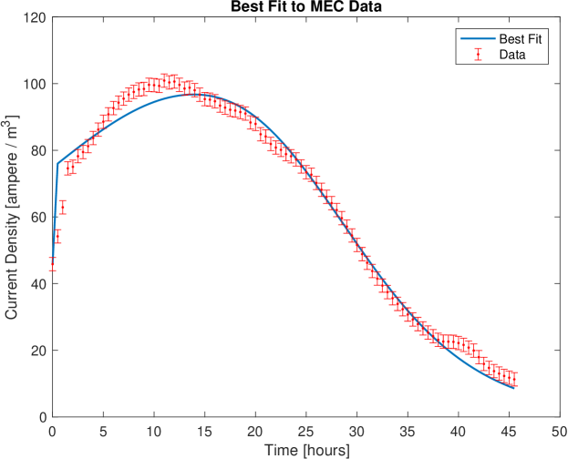
Figure 2: Comparison of best fit current density with data from a batch of the acetate fed MEC. The best fit curve for current density (in ampere/m^3) is shown as a solid blue line. Experimental data is depicted as a series of red circles. Error bars show the measurement error, $\pm 2$ ampere/m^3.

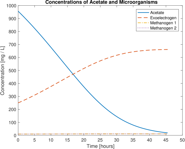
Figure 3: Best fit concentrations of acetate, exoelectrogens, and methanogens in mg/L. Acetate is represented by a solid blue line. Exoelectrogen concentration is shown as a dashed red line. Methanogen concentrations in biofilms 1 and 2 are depicted by a dashed-dot yellow line and a dotted purple line, respectively.

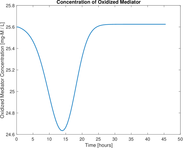
Figure 4: Solution of oxidized mediator concentration (out of $M_{\text{total}}=25.625$ mg/L). The initial conditions were chosen by solving the algebraic equation for the initial exoelectrogen concentration, $X_{e}(0)$, given initial conditions for oxidized mediator concentration and current density. $I_{\text{density}}(0)$ was experimentally determined. $M_{\text{ox}}(0)=25.6$ was chosen to provide a smooth curve for the oxidized mediator concentration.

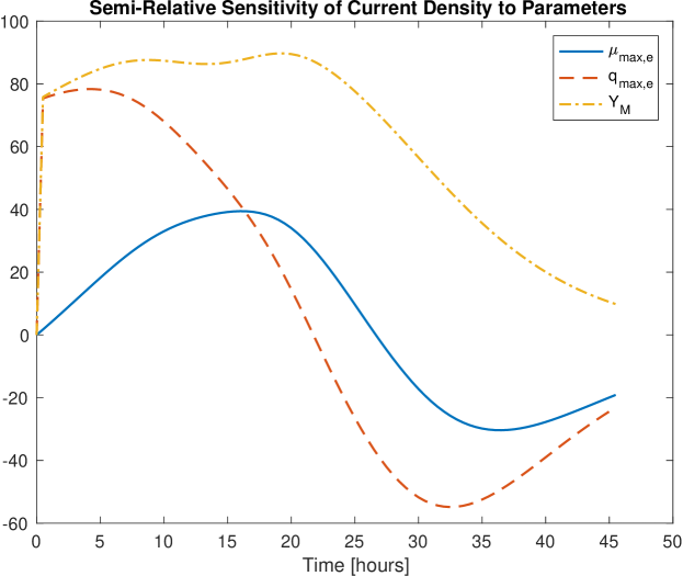
Figure 5: Semi-relative sensitivity of current density with respect to fitted parameters. Sensitivity to $\mu_{\text{max},e}$ is shown as a solid blue line, sensitivity to $q_{\text{max},e}$ is depicted as a dashed red line, and sensitivity to $Y_{M}$ is presented as a dashed-dot yellow line. Increasing either $q_{\text{max},e}$ or $Y_{M}$ will significantly increase current density during the first few hours of the experiment. This effect tapers off over time for $Y_{M}$. For $q_{\text{max},e}$, the effect is eventually reversed. Between $t=22$ and 45 hours, increasing $q_{\text{max},e}$ will decrease current density. Increasing $\mu_{\text{max},e}$ will increase current density before $t=27$ and decrease current density afterwards, although the effects are less pronounced.

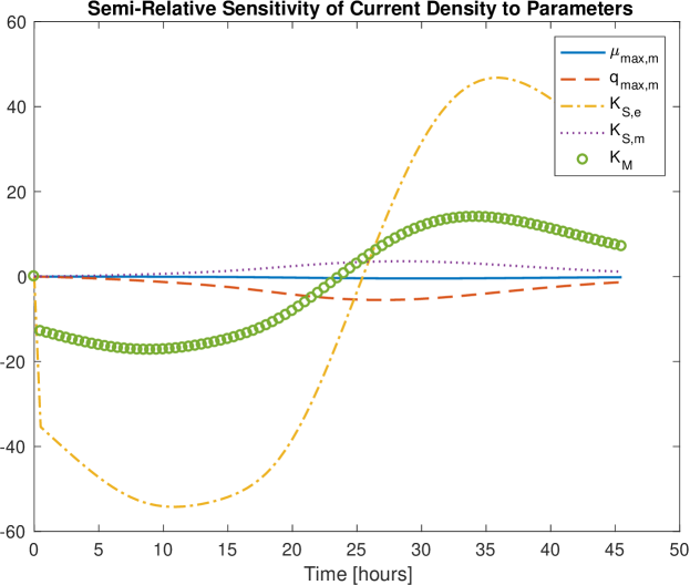
Figure 6: Semi-relative sensitivity of current density with respect to methanogen growth and consumption parameters and the three half rate constants. These parameters could not be identified. Sensitivity $\mu_{\text{max},m}$ is shown as a solid blue line, sensitivity to $q_{\text{max},m}$ is depicted as a dashed red line, sensitivity to $K_{S,e}$ is pictured as a dashed-dot yellow line, sensitivity to $K_{S,m}$ is pictured as a dotted purple line, and sensitivity to $K_{M}$ is pictured as a series of green circles. $\mu_{\text{max},m}$, $q_{\text{max},m}$, and $K_{S,m}$ do not have a significant influence on current density because methanogen concentration is relatively small in the experiment. Increasing $K_{S,e}$ would significantly decrease the current density before $t=25$ and would increase current density later. Modifying $K_{M}$ has similar but more moderate effects.

4 Bifurcation Analysis in Dilution Rate

Before presenting the bifurcation results, we provide a brief review of stability of equilibria and bifurcations in DAEs. The model in equations (6) - (11) can be represented as a regular, semi-explicit, index-1 DAE

(22) $$y^{\prime}= \,f(y,z),$$

$$0= \,g(y,z),$$

where $f:\mathbb{R}^{n+m}\rightarrow\mathbb{R}^{n}$ and $g:\mathbb{R}^{n+m}\rightarrow\mathbb{R}^{m}$. We will call a point regular for the semi-explicit DAE (22) if and only if $g(y,z)=0$ and $g_{z}(y,z)$ defines a nonsingular matrix [33, 34]. At a regular point, we can differentiate the algebraic part of (22), as long as $g\in C^{1}$, to obtain what is known as the underlying ODE

$$y^{\prime} =f(y,z)$$

$$z^{\prime} =-g_{z}^{-1}(y,z)g_{y}(y,z)f(y,z).$$

The fact that only one differentiation is required at a regular point defines (22) as an index-1 DAE. Alternatively, regularity at $(y,z)$ allows us to use the implicit function theorem to conclude the existence of a map $z=\phi(y)$ near $(y,z)$ and to describe behavior on the differential solution manifold $g(y,z)=0$ by

(23) $$y^{\prime}=f(y,\phi(y)).$$

This is known as the reduced ODE [33, 2].

Equilibrium points of (22) satisfy both $f(y,z)=0$ and $g(y,z)=0$. After defining $\hat{f}(y)=f(y,\phi(y))$, one can use the implicit function theorem and derivatives of (22) to show that linear stability of equation (23) at regular equilibria is determined by the Schur complement of the lower right block of the Jacobian matrix of $[f,g]^{T}$ [38, 2, 32]. In particular,

(24) $$\hat{f}_{y}=f_{y}-f_{z}g_{z}^{-1}g_{y}.$$

Therefore a regular equilibrium of (22) is asymptotically stable if all the eigenvalues of $f_{y}-f_{z}g_{z}^{-1}g_{y}$ have negative real part. Computing $f_{y}-f_{z}g_{z}^{-1}g_{y}$ is problematic at singular points where $g_{z}(y,z)$ is not invertible. However, the spectrum of this matrix is the same as the spectrum of the matrix pencil $\{E,-J\}=\{\lambda E-J:\lambda\in\mathbb{C}\}$ given by

$$E=\begin{bmatrix}I&0\\ 0&0\end{bmatrix}\text{ and }J=\begin{bmatrix}f_{y}&f_{z}\\ g_{y}&g_{z}\end{bmatrix}.$$

One could also use the fact that an equilibrium of the DAE (22) is asymptotically stable if the spectrum of the matrix pencil, $\sigma(\{E,-J\})=\{\lambda\in\mathbb{C}$ : $\text{det}(\lambda E-J)=0\}$, consists of elements with negative real part [33]. It is worth noting that the matrix pencil can be used to characterize stability for a generic DAE. For more information, see the exposition by Rabier and Rheinboldt [30] or the discussion with applications to circuits by Riaza [34]. For the MEC model,

$$g_{z}(y,z)=-R_{\text{int}}-\frac{RT}{\beta mFA_{\text{sur},A}i_{0}\sqrt{1+\left(\frac{I_{\text{MEC}}}{A_{\text{sur},A}i_{0}}\right)^{2}}}<0$$

is always nonsingular. Therefore, if $f(y,z)=g(y,z)=0$, we must have a regular equilibrium point and the equilibrium is asymptotically stable if the eigenvalues of $f_{y}-f_{z}g_{z}^{-1}g_{y}$ all have negative real part.

In a batch-cycle MEC, the dilution rate, $D=F_{\text{in}}/V$, is zero and equation (6) tells us that $\frac{dS}{dt}\leq 0$. In particular, $\frac{dS}{dt}=0$ only if either $S(t)=0$ or $X_{m,1}(t)=X_{e}(t)=X_{m,2}(t)=0$. If $S(t)=0$, then for each bacteria compartment $i$, $X_{i}(t)=X_{i}(0)e^{-K_{d,i}t}$. In either case $\lim_{t\rightarrow\infty}X_{i}(t)=0$. The remaining system becomes

$$\frac{dM_{\text{ox}}}{dt} =\frac{\gamma}{VmF_{2}}I_{\text{MEC}}(t),$$

$$I_{\text{MEC}}(t)R_{\text{int}}(t) =E_{\text{applied}}+E_{\text{CEMF}}-\frac{R_{1}T}{mF_{1}}\ln\left(\frac{M_{\text{total}}}{M_{\text{total}}-M_{\text{ox}}(t)}\right)-\frac{R_{1}T}{\beta mF_{1}}\text{arcsinh}\left(\frac{I_{\text{MEC}}(t)}{A_{\text{sur,A}}i_{0}}\right).$$

For the parameters in Table 1 , the system has a line of equilibria at

$$\{S,X_{m,1},X_{e},X_{m,2},M_{\text{ox}},I_{\text{MEC}}\}=\{S,0,0,0,M^{*},0\}$$

where $M^{*}$ is approximately equal to, but less than $M_{\text{total}}$ to satisfy the constraint. For instance, with the initial conditions, $\{S(0),X_{m,1}(0),X_{e}(0),X_{m,2}(0),M_{\text{ox}}(0),I_{MEC}(0)\}=\{956,10,250,10,5,0.006123\}$, the system approaches

$$\{S,X_{m,1},X_{e},X_{m,2},M_{\text{ox}},I_{\text{MEC}}\}=\{0,0,0,0,M^{*},0\}$$

with $|M^{*}-M_{\text{total}}|=4.16\times 10^{-8}$. This is a nonhyperbolic equilibrium. The spectrum of the matrix pencil (also of the Schur complement) has one zero eigenvalue:

$$\sigma(\{E,-J\})=\{-5.099\times 10^{8},-0.04,-0.002,-0.002,0\}.$$

This point lies on a line of stable equilibria in the direction $\{1,0,0,0,0,0\}$ with $\frac{dS}{dt}=0$. The substrate can take any value at equilibrium if the microorganism concentrations are zero, so any point

$$\{S,X_{m,1},X_{e},X_{m,2},M_{\text{ox}},I_{\text{MEC}}\}=\{S^{*},0,0,0,M^{*},0\}$$

can be a stable equilibrium point for the MEC system when $D=0$.

In a continuous-flow MEC, the dilution rate is non-zero and equation (6) tells us that there may be equilibria with positive concentrations of acetate. In this scenario, we hope to find a stable equilibrium with positive current, so that we can maintain long term current density and hydrogen production. We expect from simple mathematical models of chemostats that such equilibria exist for large enough flow rates [8, 36]. We demonstrate that two transcritical bifurcations in the dilution rate parameter cause this equilibrium to switch from competitive exclusion by methanogens in biofilm 2 to coexistence and then to competitive exclusion by exoelectrogens. When the dilution rate is large enough, the stable equilibrium has positive nonzero current density of at least 5 ampere/m^3. These results are depicted in Figures 7 and 8.

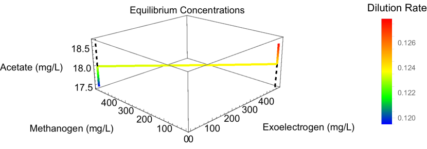
Figure 7: Stable equilibria are depicted by solid colored lines and unstable equilibria are depicted by black dashed lines. The value of the dilution rate, $D$, increases from left to right as shown by the color bar. As $D$ increases, the first transcritical bifurcation moves the stable equilibrium from a curve with no exoelectrogens to the curve of coexistence. The second transcritical bifurcation moves the stable equilibrium from the line of coexistence to a line with no methanogens. In other words, increasing D moves the stable equilibrium through three regimes: (1) competitive exclusion by methanogens, (2) coexistence, and (3) competitive exclusion by exoelectrogens.

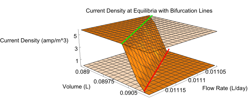
Figure 8: Stable equilibria are depicted by the solid surface and unstable equilibria are depicted by the transparent planes. The dilution rate equals the flow rate divided by the volume, D = Fin/V ; increasing either of these parameters passes the stable equilibrium through three regimes, separated by two transcritical bifurcations. Note that the flow rate and volume axes show decreasing values for a better perspective. For low values of D, there is competitive exclusion by methanogens, so the equilibria lie in a plane where the current is zero. As D increases, a transcritical bifurcation, depicted by the red line, moves the stable equilibrium onto a plane of coexistence where current density increases with D. As D increases further, a second transcritical bifurcation, depicted by the green line, moves the stable equilibrium onto a plane with competitive exclusion by exoelectrogens where the current density at the stable equilibrium is more than 5 amp / m³.

Consider the parametrized DAE,

(25) $$y^{\prime}= f(y,z,p),$$

$$0= g(y,z,p).$$

From Sotomayor’s theorem, we know that a saddle node bifurcation occurs at a nonhyperbolic equilibrium with a geometrically simple eigenvalue when certain nondegeneracy and transversality conditions are satisfied [37, 17, 23]. When the transversality condition is not satisfied, a transcritical bifurcation may occur. For DAEs, we do not necessarily know the Jacobian of the reduced ODE (23) near an equilibrium $(y^{*},z^{*},p^{*})$. However, we can apply the bifurcation conditions to the Schur complement, $f_{y}-f_{z}g_{z}^{-1}g_{y}$, as discussed in equation (24). To be precise, for the parametrized DAE (25), suppose that $f_{y}-f_{z}g_{z}^{-1}g_{y}$ has one geometrically simple zero eigenvalue that is the only eigenvalue on the imaginary axis. Furthermore, suppose that this eigenvalue has right eigenvector $v$ and left eigenvector $w$. Then a transcritical bifurcation occurs in the parameter $p$ at $(y^{*},z^{*},p^{*})$ if the following three conditions are satisfied.

Condition 4.1.

$w^{T}(f_{p}-f_{y}g_{y}^{-1}g_{p})=0$.

Condition 4.2.

$w^{T}[(f_{p}-f_{y}g_{y}^{-1}g_{p})_{y}v]\neq 0$.

Condition 4.3.

$w^{T}[(f_{y}-f_{z}g_{z}^{-1}g_{y})_{y}(v,v)]\neq 0$.

With the parameters fit to the MEC data, $\{\mu_{\text{max},e},q_{\text{max},e},Y_{M}\}=\{2.43,4.82,40.7\}$, a transcritical bifurcation occurs in the dilution rate, at $D=0.1233388$. Below this parameter value, the stable equilibrium contains only methanogens in biofilm 2. However, at this parameter value, the equilibrium point

$$\{S,X_{m,1},X_{e},X_{m,2},M_{\text{ox}},I_{\text{MEC}}\}=\{17.996,859.14,0,471.64,25.625,0\}$$

has eigenvalues

$$\{-5.099\times 10^{8},-6.406,-0.3037,-0.1666,3.036\times 10^{-17}\}$$

where the smallest eigenvalue has left eigenvector $w=<0,0,1,0,0>^{T}$ and right eigenvector

$$v=<-0.0001481,-0.0001507,0.7070,-0.7072,-4.982\times 10^{-9}>.$$

The four conditions for a transcritical bifurcation are satisfied since the smallest eigenvalue is zero up to machine precision and

$$w^{T}(f_{p}-f_{y}g_{y}^{-1}g_{p}) =0,$$

$$w^{T}[(f_{p}-f_{y}g_{y}^{-1}g_{p})_{y}v] =0.9161,$$

$$w^{T}[(f_{y}-f_{z}g_{z}^{-1}g_{y})_{y}(v,v)] =-0.0003499.$$

Beyond this dilution rate, the stable equilibrium briefly lies on a curve of coexistence between methanogens and exoelectrogens in biofilm 2. However, another transcritical bifurcation at $D=0.1240194$ switches stability to a third curve with only exoelectrogens in biofilm 2. Figure 7 shows the stable equilibrium concentrations moving between three lines in (Exoelectrogen, Methanogen, Acetate) space as $D$ increases. Unstable equilibria are depicted as dashed lines. Figure 8 provides another perspective, showing that the stable equilibrium moves between three planes in (Flow Rate, Volume, Current Density) space as $D$ increases. In both cases, the stable equilibria move through three regimes as $D$ increases: (1) competitive exclusion by methanogens, (2) coexistence, and (3) competitive exclusion by exoelectrogens. For these 90 mL MECs, the dilution rate $D=F_{\text{in}}/V=0.124$ corresponds to a flow rate of about $F_{\text{in}}=11$ mL / day. However, the location of the bifurcations depends very much on the parameters used.

5 Discussion

The differential-algebraic sensitivity analysis in Section 3 reveals how perturbations of a single parameter influence the current density at particular times. During the first day of the experiment, the four parameters related to exoelectrogen growth, $\mu_{\text{max},e}$, $q_{\text{max},e}$, $K_{S,e}$, and $Y_{M}$ had the most influence on current. Increasing the oxidized mediator yield, $Y_{M}$, would significantly increase current throughout the experiment. In contrast, increasing the maximum exoelectrogen consumption rate, $q_{\text{max},e}$, would significantly increase the current during the first 22 hours, but decrease it later; changing the exoelectrogen half rate constant, $K_{S,e}$ would have the opposite effects of changing $q_{\text{max},e}$. Increasing the maximum exoelectrogen growth rate, $\mu_{\text{max},e}$, would moderately increase current during the first day, but decrease it later; increasing the mediator half rate constant, $K_{M}$, would have opposite effects of increasing $\mu_{\text{max},e}$ on a smaller scale. These parameter effects show that the microbial growth was closely correlated with substrate availability. The parameters related to methanogen growth, $\mu_{\text{max},m}$, $q_{\text{max},m}$, and $K_{S,m}$, had very little impact on current during experiment. This is likely due to the small methanogen population in the MECs, which is also consistent with previous findings that exoelectrogens have more affinities than acetolastic methanogens [16]. These results suggest that increasing $\mu_{\text{max},e}$, $q_{\text{max},e}$, and $Y_{M}$ or decreasing $K_{S,e}$ would result in higher peak current density. Although the methanogen populations are small in this experiment, the results also suggest that decreasing $q_{\text{max},m}$ or increasing $K_{S,m}$ could lead to higher peak current density when the methanogen population is large.

The bifurcation analysis in Section 4 shows that the dilution rate in a continuous flow MEC must be chosen carefully to ensure that the system approaches a stable equilibrium with positive current density. For the fitted parameters, the system exhibits two transcritical bifurcations. As dilution rate increases, the first bifurcation moves the stable equilibrium from a curve with competitive exclusion by methanogens to a curve with coexistence of exoelectrogens and methanogens. The second bifurcation switches stability from the curve with coexistence to a curve with competitive exclusion by exoelectrogens. This result is depicted in Figures 7 and 8. Only at high enough dilution rates will exoelectrogens be able to dominate and provide positive current density. This indicates that using the appropriate dilution rate can be an effective approach for maintaining a vibrant exoelectrogenic microbial community and maintaining stable system performance. For the 90 mL MECs considered, these bifurcations occur at dilution rates $D=F_{\text{in}}/V$ of about 0.1233 and 0.1240, corresponding to flow rates just above $F_{\text{in}}=11$ mL / day. However, the location of these bifurcations is determined by the microbial growth parameters. Although not discussed in the results, modifying parameters besides dilution rate may increase or decrease the current at the stable equilibrium.

6 Conclusion

The microbial growth and consumption parameters were not measured in the batch-cycle MEC experiment, but the results suggest that they should be considered carefully in MEC studies. These parameters, namely $\mu_{\text{max},e}$, $q_{\text{max},e}$, $K_{S,e}$, $\mu_{\text{max},m}$, $q_{\text{max},m}$, $K_{S,m}$, and $Y_{M}$, should be estimated or measured if possible, in both batch-cycle and continuous-flow MECs. In the former case, the parameter values provide information about the peak current density during each batch. In the latter case, the parameters can be used to guide design before long term operation of a continuous-flow MEC. Additionally, we have not considered the effects of different substrates and different combinations of microorganisms. If we consider another substrate, such as ethanol, the best fit values of the parameters will be different and the sensitivity analysis methods could provide additional insight. A further complication is that microbial community structure varies when different substrates are used. That is, the percentages of bacteria species that are present will depend on the substrate that is used. This means that estimates for growth and consumption parameters from one MEC study may not be reliable in another. These factors are not taken into account by this simple model, but a similar modeling approach can be used as the degradation process is comparable. We plan to model multiple substrates in future work.

Several aspects of the MEC system were overlooked in this study. We did not consider rate hydrogen production directly since we do not have a time series for either the hydrogen production rate or the population of hydrogen consuming methanogens. If we were able to measure either of those quantities, we could repeat this analysis to determine precisely which parameters exert the most influence on the hydrogen production rate itself. However, literature has shown that hydrogen production directly correlates with current generation so the findings presented in the study do represent the variation of hydrogen generation from the MEC. The DAE model has the advantage of being computationally inexpensive compared to PDE models, but the latter may provide a more accurate characterization of the biofilm beyond merely concentration in a well mixed compartment. Future work could analyze the bifurcations in biofilm concentration in the context of a PDE model.

7 Acknowledgements

HJD and DMB are partially supported by NSF grant DMS-1225878. ZJR and LL acknowledge support from NSF grant CBET-1510682 and ONR grant N000141612210. We thank Stephen Campbell for his help with questions about DAEs.

References

- [1] D. J. Batstone, J. Keller, I. Angelidaki, S. V. Kalyuzhnyi, S. G. Pavlostathis, A. Rozzi, W. T. M. Sanders, H. Siegrist, and V. A. Vavilin, The IWA Anaerobic Digestion Model No 1 (ADM1), Water Science and Technology, 45 (2002), pp. 65–73.
- [2] R. E. Beardmore, Stability and bifurcation properties of index-1 DAEs, Numerical Algorithms, 19 (1998), pp. 43–53.
- [3] K. Brenan, S. Campbell, and L. Petzold, Numerical Solution of Initial-Value Problems in Differential-Algebraic Equations, Classics in Applied Mathematics, Society for Industrial and Applied Mathematics, Jan. 1995.
- [4] D. Call and B. E. Logan, Hydrogen production in a single chamber microbial electrolysis cell lacking a membrane, Environmental Science & Technology, 42 (2008), pp. 3401–3406.
- [5] S. K. Chaudhuri and D. R. Lovley, Electricity generation by direct oxidation of glucose in mediatorless microbial fuel cells, Nature Biotechnology, 21 (2003), pp. 1229–1232.
- [6] S. R. Hansen and S. P. Hubbell, Single-nutrient microbial competition: qualitative agreement between experimental and theoretically forecast outcomes, Science (New York, N.Y.), 207 (1980), pp. 1491–1493.
- [7] A. C. Hindmarsh, P. N. Brown, K. E. Grant, S. L. Lee, R. Serban, D. E. Shumaker, and C. S. Woodward, SUNDIALS: Suite of nonlinear and differential/algebraic equation solvers, ACM Transactions on Mathematical Software (TOMS), 31 (2005), pp. 363–396.
- [8] S. Hsu, S. Hubbell, and P. Waltman, A Mathematical Theory for Single-Nutrient Competition in Continuous Cultures of Micro-Organisms, SIAM Journal on Applied Mathematics, 32 (1977), pp. 366–383.
- [9] A. Kato Marcus, C. I. Torres, and B. E. Rittmann, Conduction-based modeling of the biofilm anode of a microbial fuel cell, Biotechnology and Bioengineering, 98 (2007), pp. 1171–1182.
- [10] H. Liu, S. Grot, and B. E. Logan, Electrochemically Assisted Microbial Production of Hydrogen from Acetate, Environmental Science & Technology, 39 (2005), pp. 4317–4320.
- [11] B. E. Logan, Exoelectrogenic bacteria that power microbial fuel cells, Nature Reviews Microbiology, 7 (2009), pp. 375–381.
- [12] B. E. Logan, B. Hamelers, R. Rozendal, U. Schröder, J. Keller, S. Freguia, P. Aelterman, W. Verstraete, and K. Rabaey, Microbial fuel cells: Methodology and technology, Environmental Science & Technology, 40 (2006), pp. 5181–5192.
- [13] L. Lu, D. Hou, Y. Fang, Y. Huang, and Z. J. Ren, Nickel based catalysts for highly efficient H2 evolution from wastewater in microbial electrolysis cells, Electrochimica Acta, 206 (2016), pp. 381–387.
- [14] L. Lu, D. Hou, X. Wang, D. Jassby, and Z. J. Ren, Active H2 Harvesting Prevents Methanogenesis in Microbial Electrolysis Cells, Environmental Science & Technology Letters, 3 (2016), pp. 286–290.
- [15] L. Lu, N. Ren, D. Xing, and B. E. Logan, Hydrogen production with effluent from an ethanol-h2-coproducing fermentation reactor using a single-chamber microbial electrolysis cell, Biosensors and Bioelectronics, 24 (2009), pp. 3055–3060.
- [16] L. Lu and Z. J. Ren, Microbial electrolysis cells for waste biorefinery: A state of the art review, Bioresource Technology, 215 (2016), pp. 254–264.
- [17] J. Meiss, Differential Dynamical Systems, Revised Edition, Mathematical Modeling and Computation, Society for Industrial and Applied Mathematics, Jan. 2017.
- [18] J. Monod, Recherches sur la croissance des cultures bactériennes, Hermann, 1958. Google-Books-ID: Gi9rAAAAMAAJ.
- [19] D. A. Noren and M. A. Hoffman, Clarifying the butler-volmer equation and related approximations for calculating activation losses in solid oxide fuel cell models, Journal of Power Sources, 152 (2005), pp. 175–181.
- [20] A. Novick and L. Szilard, Description of the Chemostat, Science, 112 (1950), pp. 715–716.
- [21] V. B. Oliveira, M. Simões, L. F. Melo, and A. M. F. R. Pinto, Overview on the developments of microbial fuel cells, Biochemical Engineering Journal, 73 (2013), pp. 53–64.
- [22] V. M. Ortiz-Martínez, M. J. Salar-García, A. P. de los Ríos, F. J. Hernández-Fernández, J. A. Egea, and L. J. Lozano, Developments in microbial fuel cell modeling, Chemical Engineering Journal, 271 (2015), pp. 50–60.
- [23] L. Perko, Differential Equations and Dynamical Systems, Springer, 2001.
- [24] C. Picioreanu, I. M. Head, K. P. Katuri, M. C. M. van Loosdrecht, and K. Scott, A computational model for biofilm-based microbial fuel cells, Water Research, 41 (2007), pp. 2921–2940.
- [25] C. Picioreanu, M. C. M. van Loosdrecht, T. P. Curtis, and K. Scott, Model based evaluation of the effect of pH and electrode geometry on microbial fuel cell performance, Bioelectrochemistry, 78 (2010), pp. 8–24.
- [26] C. Picioreanu, M. C. M. van Loosdrecht, K. P. Katuri, K. Scott, and I. M. Head, Mathematical model for microbial fuel cells with anodic biofilms and anaerobic digestion, Water Science and Technology: A Journal of the International Association on Water Pollution Research, 57 (2008), pp. 965–971.
- [27] R. Pinto, B. Srinivasan, M.-F. Manuel, and B. Tartakovsky, A two-population bio-electrochemical model of a microbial fuel cell, Bioresource Technology, 101 (2010), pp. 5256–5265.
- [28] R. P. Pinto, B. Srinivasan, A. Escapa, and B. Tartakovsky, Multi-population model of a microbial electrolysis cell, Environmental Science & Technology, 45 (2011), pp. 5039–5046.
- [29] K. Rabaey and R. Rozendal, Microbial electrosynthesis - revisiting the electrical route for microbial production, Nature Reviews Microbiology, 8 (2010), pp. 706–716.
- [30] P. J. Rabier and W. C. Rheinboldt, Theoretical and numerical analysis of differential-algebraic equations, in Handbook of Numerical Analysis, P. Ciarlet and J. Lions, eds., no. v. 8 in Handbook of Numerical Analysis, North-Holland, 1990.
- [31] D. Recio-Garrido, M. Perrier, and B. Tartakovsky, Modeling, optimization and control of bioelectrochemical systems, Chemical Engineering Journal, 289 (2016), pp. 180–190.
- [32] S. Reich, On the local qualitative behavior of differential-algebraic equations, Circuits, Systems and Signal Processing, 14 (1995), pp. 427–443.
- [33] R. Riaza, Stability Issues in Regular and Noncritical Singular DAEs, Acta Applicandae Mathematica, 73 (2002), pp. 301–336.
- [34] R. Riaza, Differential-Algebraic Systems: Analytical Aspects and Circuit Applications, World Scientific, 2008.
- [35] R. A. Rozendal, H. V. M. Hamelers, G. J. W. Euverink, S. J. Metz, and C. J. N. Buisman, Principle and perspectives of hydrogen production through biocatalyzed electrolysis, International Journal of Hydrogen Energy, 31 (2006), pp. 1632–1640.
- [36] H. L. Smith and P. Waltman, The Theory of the Chemostat: Dynamics of Microbial Competition, Cambridge University Press, Jan. 1995. Google-Books-ID: wFLdVo89vq8C.
- [37] J. Sotomayor, Generic Bifurcations of Dynamical Systems, in Dynamical Systems, M. M. Peixoto, ed., Academic Press, 1973, pp. 561–582.
- [38] V. Venkatasubramanian, H. Schattler, and J. Zaborszky, Local bifurcations and feasibility regions in differential-algebraic systems, IEEE Transactions on Automatic Control, 40 (1995), pp. 1992–2013.
- [39] H. Wang and Z. J. Ren, A comprehensive review of microbial electrochemical systems as a platform technology, Biotechnology Advances, 31 (2013), pp. 1796–1807.
- [40] X.-C. Zhang and A. Halme, Modelling of a microbial fuel cell process, Biotechnology Letters, 17 (1995), pp. 809–814.