Improving the accuracy of the fast inverse square root algorithm

Abstract

We present improved algorithms for fast calculation of the inverse square root for single-precision floating-point numbers. The algorithms are much more accurate than the famous fast inverse square root algorithm and have the same or similar computational cost. The main idea of our work consists in modifying the Newton-Raphson method and demanding that the maximal error is as small as possible. The modification can be applied when the distribution of Newton-Raphson corrections is not symmetric (e.g., if they are non-positive functions).

Keywords: floating-point arithmetic; inverse square root; magic constant; Newton-Raphson method

1 Introduction

Floating-point arithmetic has became widely used in many applications such as 3D graphics, scientific computing and signal processing [1, 2, 3, 4, 5], implemented both in hardware and software [6, 7, 8, 9, 10]. Many algorithms can be used to approximate elementary functions, including the inverse square root [1, 2, 10, 11, 12, 13, 14, 15, 16, 17, 18, 19]. All of these algorithms require initial seed to start the approximation. The more accurate is the initial seed, the less iterations is required to compute the function. In most cases the initial seed is obtained from a look-up table (LUT) which is memory consuming. The inverse square root function is of particular importance because of it is widely used in 3D computer graphics especially in lightning reflections [20, 21, 22]. In this paper we consider an algorithm for computing the inverse square root for single-precision IEEE Standard 754 floating-point numbers (type float) using so the called magic constant instead of LUT [23, 24, 25, 26].

1.	float InvSqrt(float x){
2.		float halfnumber = 0.5f * x;
3.		int i = *(int*) &x;
4.		i = R-(i$>>$1);
5.		x = *(float*)&i;
6.		x = x*(1.5f-halfnumber*x*x);
7.		x = x*(1.5f-halfnumber*x*x);
8.		return x ;
9.	}

The code InvSqrt realizes a fast algorithm for calculation of the inverse square root. It consists of two main parts. Lines 4 and 5 produce in a very cheap way a quite good zeroth approximation of the inverse square root of given positive floating-point number $x$. Lines 6 and 7 apply the Newton-Raphson corrections.

The algorithm InvSqrt has numerous applications, see [27, 28, 29, 30, 31, 32, 33, 34, 35, 36, 37, 38, 39]. The most important among them is 3D computer graphics, where normalization of vectors is ubiquitous. InvSqrt is characterized by a high speed, more that 3 times higher than in computing the inverse square root using library functions. This property is discussed in detail in [41]. The errors of the fast inverse square root algorithm depend on the choice of the “magic constant” $R$. In several theoretical papers [24, 40, 41, 42, 43] (see also the Eberly’s monograph [20]) attempts were made to determine analytically the optimal value of the magic constant (i.e., to minimize errors). In general, this optimal value can depend on the number of iterations, which is a general phenomenon [44]. The derivation and comprehensive mathematical description of all steps of the fast inverse square root algorithm is given in our recent paper [45]. It is worthwhile to notice that a magic constant appearing in the Ziv’s rounding test [46] has been recently derived in an analytic way as well [47].

In this paper we develop our analytical approach [45] to construct improved algorithms for computing the inverse square root. The first part of the code will be the same (but we treat $R$ as a free parameter to be determined by minimization of the relative error). The second part of the code will be changed significantly. In fact, we propose a modification of the Newton-Raphson formulae which has the same or similar computational cost but improves the accuracy by several times.

The magic constant in the InvSqrt code serves as a low-cost way of generating a reasonably accurate first approximation of the inverse square root. We are going to insert other “magic constants” into this code in order to increase the accuracy of the algorithm without extra costs.

2 Algorithm InvSqrt. An analytical approach

In this section we shortly present main results of [45]. We confine ourselves to positive floating-point numbers

$$x=(1+m_{x})2^{e_{x}}$$ (2.1)

where $m_{x}\in[0,1)$ and $e_{x}$ is an integer. In the case of the IEEE-754 standard, a floating-point number is encoded by 32 bits. The first bit corresponds to a sign (in our case this bit is simply equal to zero), the next 8 bits correspond to an exponent $e_{x}$ and the last 23 bits encodes a mantissa $m_{x}$. The integer encoded by these 32 bits, denoted by $I_{x}$, is given by

$$I_{x}=N_{m}(B+e_{x}+m_{x})$$ (2.2)

where $N_{m}=2^{23}$ and $B=127$ (thus $B+e_{x}=1,2,\ldots,254$). The lines 3 and 5 of the InvSqrt code interprete a number as an integer (2.2) or float (2.1), respectively. The lines 4, 6 and 7 of the code can be written as

$$\begin{array}[]{l}I_{y_{0}}=R-\lfloor I_{x}/2\rfloor,\\[3.87498pt] y_{1}=\frac{1}{2}y_{0}(3-y_{0}^{2}x),\\[3.87498pt] y_{2}=\frac{1}{2}y_{1}(3-y_{1}^{2}x).\end{array}$$ (2.3)

The first equation produces, in a surprisingly simple way, a good zeroth approximation $y_{0}$ of the inverse square root $y=1/\sqrt{x}$. The next equations can be easily recognized as Newton-Raphson corrections. We point out that the code InvSqrt is invariant with respect to the scaling

$$x\rightarrow\tilde{x}=2^{-2n}x,\qquad y_{k}\rightarrow\tilde{y}_{k}=2^{n}y_{k}\quad(k=0,1,2),$$ (2.4)

like the equality $y=1/\sqrt{x}$ itself. Therefore, without loss of the generality, we can confine our analysis to the interval

$$\tilde{A}:=[1,4).$$ (2.5)

The tilde will denote quantities defined on this interval. In [45] we have shown that the function ${\tilde{y}}_{0}$ defined by the first equation of (2.3) can be approximated with a very good accuracy by the piece-wise linear function $\tilde{y}_{00}$ given by

$$\tilde{y}_{00}(\tilde{x},t)=\left\{\begin{array}[]{ll}\displaystyle-\frac{1}{4}\tilde{x}+\frac{3}{4}+\frac{1}{8}t&\text{for}\ \ \tilde{x}\in[1,2)\\[7.74997pt] \displaystyle-\frac{1}{8}\tilde{x}+\frac{1}{2}+\frac{1}{8}t&\text{for}\ \ \tilde{x}\in[2,t)\\[7.74997pt] \displaystyle-\frac{1}{16}\tilde{x}+\frac{1}{2}+\frac{1}{16}t&\text{for}\ \ \tilde{x}\in[t,4)\end{array}\right.$$ (2.6)

where

$$t=2+4m_{R}+2N_{m}^{-1},$$ (2.7)

and $m_{R}:=N_{m}^{-1}R-\lfloor N_{m}^{-1}R\rfloor$ ($m_{R}$ is a mantissa of the floating-point numbers corresponding to $R$). We assumed $m_{R}<\frac{1}{2}$ and, as a results, we obtained $e_{R}=63$ and $t>2$.

The only difference between $y_{0}$ produced by the code InvSqrt and $y_{00}$ given by (2.6) is the definition of $t$, because $t$ related to the code depends (although in a negligible way) on $x$. Namely,

$$|{\tilde{y}}_{00}-{\tilde{y}}_{0}|\leqslant\frac{1}{4}N_{m}^{-1}=2^{-25}\approx 2.98\cdot 10^{-8}.$$ (2.8)

Taking into account the invariance (2.4), we obtain

$$\left|\frac{y_{00}-y_{0}}{y_{0}}\right|\leqslant 2^{-24}\approx 5.96\cdot 10^{-8}.$$ (2.9)

These estimates do not depend on $t$ (in other words, they do not depend on $R$). The relative error of the zeroth approximation (2.6) is given by

$$\tilde{\delta}_{0}(\tilde{x},t)=\sqrt{\tilde{x}}\ {\tilde{y}}_{00}(\tilde{x},t)-1$$ (2.10)

This is a continuous function with local maxima at

$$\tilde{x}_{0}^{I}=(6+t)/6,\quad\tilde{x}_{0}^{II}=(4+t)/3,\quad\tilde{x}_{0}^{III}=(8+t)/3,$$ (2.11)

given respectively by

$$\begin{array}[]{l}\displaystyle\tilde{\delta}_{0}(\tilde{x}_{0}^{I},t)=-1+\frac{1}{2}\left(1+\frac{t}{6}\right)^{3/2}\ ,\\[7.74997pt] \displaystyle\tilde{\delta}_{0}(\tilde{x}_{0}^{II},t)=-1+2\left(\frac{1}{3}\left(1+\frac{t}{4}\right)\right)^{3/2}\ ,\\[7.74997pt] \displaystyle\tilde{\delta}_{0}(\tilde{x}_{0}^{III},t)=-1+\left(\frac{2}{3}\left(1+\frac{t}{8}\right)\right)^{3/2}\ .\end{array}$$ (2.12)

In order to study global extrema of $\tilde{\delta}_{0}(\tilde{x},t)$ we need also boundary values:

$$\begin{array}[]{l}\displaystyle\tilde{\delta}_{0}(1,t)=\displaystyle\tilde{\delta}_{0}(4,t)=\frac{1}{8}\left(t-4\right),\\[7.74997pt] \displaystyle\tilde{\delta}_{0}(2,t)=\frac{\sqrt{2}}{4}\left(1+\frac{t}{2}\right)-1,\\[7.74997pt] \displaystyle\tilde{\delta}_{0}(t,t)=\frac{\sqrt{t}}{2}-1,\\[7.74997pt] \end{array}$$ (2.13)

which are, in fact, local minima. Taking into account

$$\begin{array}[]{l}\displaystyle\tilde{\delta}_{0}(1,t)-\tilde{\delta}_{0}(t,t)=\frac{1}{8}\left(\sqrt{t}-2\right)^{2}\geqslant 0\ ,\\[7.74997pt] \displaystyle\tilde{\delta}_{0}(2,t)-\tilde{\delta}_{0}(t,t)=\frac{\sqrt{2}}{8}\left(\sqrt{t}-\sqrt{2}\right)^{2}\geqslant 0,\end{array}$$ (2.14)

we conclude that

$$\min_{\tilde{x}\in\tilde{A}}\tilde{\delta}_{0}(\tilde{x},t)=\tilde{\delta}_{0}(t,t)<0.$$ (2.15)

Because $\tilde{\delta}_{0}(\tilde{x}_{0}^{III},t)<0$ for $t\in(2,4)$, the global maximum is one of the remaining local maxima:

$$\max_{\tilde{x}\in\tilde{A}}\tilde{\delta}_{0}(\tilde{x},t)=\max\{\tilde{\delta}_{0}(\tilde{x}_{0}^{I},t),\tilde{\delta}_{0}(\tilde{x}_{0}^{II},t)\}.$$ (2.16)

Therefore,

$$\max_{x\in\tilde{A}}|\tilde{\delta}_{0}(\tilde{x},t)|=\max\{|\tilde{\delta}_{0}(t,t)|,\tilde{\delta}_{0}(\tilde{x}_{0}^{I},t),\tilde{\delta}_{0}(\tilde{x}_{0}^{II},t)\}.$$ (2.17)

In order to minimize this value with respect to $t$, i.e., to find $t_{0}^{r}$ such that

$$\max_{x\in\tilde{A}}|\tilde{\delta}_{0}(\tilde{x},t_{0}^{r})|<\max_{x\in\tilde{A}}|\tilde{\delta}_{0}(\tilde{x},t)|\qquad\text{for}t\neq t_{0}^{r},$$ (2.18)

we observe that $|\tilde{\delta}_{0}(t,t)|$ is a decreasing function of $t$, while both maxima ($\tilde{\delta}_{0}(\tilde{x}_{0}^{I},t)$ and $\tilde{\delta}_{0}(\tilde{x}_{0}^{II},t)$) are increasing functions. Therefore, it is sufficient to find $t=t_{0}^{I}$ and $t=t_{0}^{II}$ such that

$$|\tilde{\delta}_{0}(t_{0}^{I},t_{0}^{I})|=\tilde{\delta}_{0}(\tilde{x}_{0}^{I},t_{0}^{I})\ ,\qquad|\tilde{\delta}_{0}(t_{0}^{II},t_{0}^{II})|=\tilde{\delta}_{0}(\tilde{x}_{0}^{II},t_{0}^{II}),$$ (2.19)

and to choose the greater of these two values. In [45] we have shown that

$$|\tilde{\delta}_{0}(t_{0}^{I},t_{0}^{I})|<|\tilde{\delta}_{0}(t_{0}^{II},t_{0}^{II})|.$$ (2.20)

Therefore $t_{0}^{r}=t_{0}^{II}$ and

$$\tilde{\delta}_{0\max}:=\min_{t\in(2,4)}\left(\max_{x\in\tilde{A}}|\tilde{\delta}_{0}(\tilde{x},t)|\right)=|\tilde{\delta}_{0}(t_{0}^{r},t_{0}^{r})|.$$ (2.21)

The following numerical values result from these calculations [45]:

$$t_{0}^{r}\approx 3.7309796,\qquad R_{0}=0x5F37642F,\qquad\tilde{\delta}_{0\max}\approx 0.03421281.$$ (2.22)

Newton-Raphson corrections for the zeroth approximation given by $\tilde{y}_{00}$ will be denoted by $\tilde{y}_{0k}$ ($k=1,2,\ldots$), in particular:

$$\begin{array}[]{l}\tilde{y}_{01}(\tilde{x},t)=\frac{1}{2}\tilde{y}_{00}(\tilde{x},t)(3-\tilde{y}_{00}^{2}(\tilde{x},t)\,\tilde{x}),\\[7.74997pt] \tilde{y}_{02}(\tilde{x},t)=\frac{1}{2}\tilde{y}_{01}(\tilde{x},t)(3-\tilde{y}_{01}^{2}(\tilde{x},t)\,\tilde{x}).\end{array}$$ (2.23)

and the corresponding relative error functions will be denoted by $\tilde{\delta}_{k}(\tilde{x},t)$:

$$\tilde{\delta}_{k}(\tilde{x},t):=\frac{\tilde{y}_{0k}(\tilde{x},t)-\tilde{y}}{\tilde{y}}=\sqrt{\tilde{x}}\tilde{y}_{0k}(\tilde{x},t)-1,\qquad(k=0,1,2,\ldots),$$ (2.24)

where we included also the case $k=0$, see (2.10). The obtained approximations of the inverse square root depend on the parameter $t$ directly related to the magic constant $R$. The value of this parameter can be estimated by analysing the relative error of $\tilde{y}_{0k}(\tilde{x},t)$ with respect to $1/\sqrt{\tilde{x}}$. As the best estimation we consider $t=t_{k}^{(r)}$ minimizing the relative error $\tilde{\delta}_{k}(\tilde{x},t)$:

$$\forall_{t\neq t_{k}^{(r)}}\left(\tilde{\delta}_{k\max}\equiv\max_{\tilde{x}\in\tilde{A}}|\tilde{\delta}_{k}(\tilde{x},t_{k}^{(r)})|<\max_{\tilde{x}\in\tilde{A}}|\tilde{\delta}_{k}(\tilde{x},t)|\right).$$ (2.25)

We point out that in general the optimum value of the magic constant can depend on the number of Newton-Raphson corrections. Calculations carried out in [45] gave the following results:

$$\begin{array}[]{l}t_{1}^{r}=t_{2}^{r}=3.7298003,\qquad R_{1}^{r}=R_{2}^{r}=0x5F375A86,\\[3.87498pt] \tilde{\delta}_{1\max}\approx 1.75118\cdot 10^{-3},\quad\tilde{\delta}_{2\max}\approx 4.60\cdot 10^{-6}.\end{array}$$ (2.26)

We omit details of the computations except one important point. Using (2.24) for expressing $\tilde{y}_{0k}$ by $\tilde{\delta}_{k}$ and $\sqrt{\tilde{x}}$ we can rewrite (2.23) as

$$\tilde{\delta}_{k}(\tilde{x},t)=-\frac{1}{2}\tilde{\delta}_{k-1}^{2}(\tilde{x},t)(3+\tilde{\delta}_{k-1}(\tilde{x},t)),\quad(k=1,2,\ldots).$$ (2.27)

The quadratic dependence on $\tilde{\delta}_{k-1}$ means that every Newton-Raphson correction improves the accuracy by several orders of magnitude, compare (2.26).

The formula (2.27) suggests another way of improving the accuracy because the functions $\tilde{\delta}_{k}$ are always non-positive for any $k\geqslant 1$. Roughly saying, we are going to shift the graph of $\tilde{\delta}_{k}$ upwards by an appropriate modification of the Newton-Raphson formula. In the next sections we describe the general idea of this modification and derive two new codes for fast and accurate computation of the inverse square root.

3 Modified Newton-Raphson formula

The formula (2.27) shows that Newton-Raphson corrections are nonpositive (see also Fig. 4 and Fig. 5 in [45]), i.e., they take values in intervals $[-{\tilde{\delta}}_{k\max},\,0]$, where $k=1,2,\ldots$. Therefore, it is natural to introduce a correction term into Newton-Raphson formulas (2.23). We expect that the corrections will be roughly half of the maximal relative error. Instead of the maximal error we introduce two parameters, $d_{1}$ and $d_{2}$. Thus we get modified Newton-Raphson formulas:

$$\begin{array}[]{l}\displaystyle\tilde{y}_{11}(\tilde{x},t,d_{1})=2^{-1}\tilde{y}_{00}(\tilde{x},t)(3-\tilde{y}_{00}^{2}(\tilde{x},t)\,\tilde{x})+\frac{d_{1}}{2\sqrt{\tilde{x}}},\\[7.74997pt] \displaystyle\tilde{y}_{12}(\tilde{x},t,d_{1},d_{2})=2^{-1}\tilde{y}_{11}(\tilde{x},t,d_{1})(3-\tilde{y}_{11}^{2}(\tilde{x},t,d_{1})\,\tilde{x})+\frac{d_{2}}{2\sqrt{\tilde{x}}},\end{array}$$ (3.1)

where we still assume the zeroth approximation in the form (2.6). The corresponding error functions,

$$\tilde{\delta}^{{}^{\prime\prime}}_{k}(\tilde{x},t,d_{1},\ldots,d_{k})=\sqrt{\tilde{x}}\,\tilde{y}_{1k}(\tilde{x},t,d_{1},\ldots,d_{k})-1,\qquad k\in\{0,1,2,\ldots\},$$ (3.2)

(where $\tilde{y}_{10}(\tilde{x},t):=\tilde{y}_{00}(\tilde{x},t)$), satisfy

$$\tilde{\delta}^{{}^{\prime\prime}}_{k}=-\frac{1}{2}\tilde{\delta}^{{}^{\prime\prime}2}_{k-1}(3+\tilde{\delta}^{{}^{\prime\prime}}_{k-1})+\frac{d_{k}}{2},$$ (3.3)

where: $\tilde{\delta}^{{}^{\prime\prime}}_{0}(\tilde{x},t)=\tilde{\delta}_{0}(\tilde{x},t)$. Note that

$$\tilde{\delta}^{{}^{\prime\prime}}_{1}(\tilde{x},t,d_{1})=\tilde{\delta}_{1}(\tilde{x},t)+\frac{1}{2}d_{1}.$$ (3.4)

In order to simplify notation we usually will supress the explicit dependence on $d_{j}$. We will write, for instance, $\tilde{\delta}^{{}^{\prime\prime}}_{2}(\tilde{x},t)$ instead of $\tilde{\delta}^{{}^{\prime\prime}}_{2}(\tilde{x},t,d_{1},d_{2})$.

The corrections of the form (3.1) will decrease relative errors in comparison with the results of earlier papers [24, 45]. We have 3 free parameters ($d_{1},d_{2}$ and $t$) to be determined by minimizing the maximal error (in principle the new parameterization can give a new estimation of the parameter $t$). By analogy to (2.25), we are going to find $t=t^{(0)}$ minimizing the error of the first correction (2.25):

$$\forall_{t\neq t^{(0)}}\max_{\tilde{x}\in\tilde{A}}|\tilde{\delta}_{1}^{{}^{\prime\prime}}(\tilde{x},t^{(0)})|<\max_{\tilde{x}\in\tilde{A}}|\tilde{\delta}^{{}^{\prime\prime}}_{1}(\tilde{x},t)|,$$ (3.5)

where, as usual, $\tilde{A}=[1,4]$.

The first of Eqs. (3.3) implies that for any $t$ the maximal value of $\tilde{\delta}^{{}^{\prime\prime}}_{1}(\tilde{x},t)$ equals $\frac{1}{2}d_{1}$ and is attained at zeros of $\tilde{\delta}^{{}^{\prime\prime}}_{0}(\tilde{x},t)$. Using results of section 2, including (2.15), (2.16), (2.20) and (2.21), we conclude that the minimum value of $\tilde{\delta}^{{}^{\prime\prime}}_{1}(\tilde{x},t)$ is attained either for $\tilde{x}=t$ or for $\tilde{x}=x_{0}^{II}$ (where there is the second maximum of $\tilde{\delta}^{{}^{\prime\prime}}_{0}(\tilde{x},t)$), i.e.,

$$\min_{\tilde{x}\in\tilde{A}}\tilde{\delta}^{{}^{\prime\prime}}_{1}(\tilde{x},t)=\min\left\{\tilde{\delta}^{{}^{\prime\prime}}_{1}(t,t),\tilde{\delta}^{{}^{\prime\prime}}_{1}(x_{0}^{II},t)\right\}$$ (3.6)

Minimization of $|\tilde{\delta}^{{}^{\prime\prime}}_{1}(\tilde{x},t)|$ can be done with respect to $t$ and with respect to $d_{1}$ (these both operations obviously commute). corresponds to

$$\underbrace{\max_{\tilde{x}\in\tilde{A}}\tilde{\delta}^{{}^{\prime\prime}}_{1}(\tilde{x},t^{(0)})}_{\tilde{\delta}^{{}^{\prime\prime}}_{1\max}}=-\min_{\tilde{x}\in\tilde{A}}\tilde{\delta}^{{}^{\prime\prime}}_{1}(\tilde{x},t^{(0)}).$$ (3.7)

Taking into account

$$\max_{\tilde{x}\in\tilde{A}}\tilde{\delta}^{{}^{\prime\prime}}_{1}(\tilde{x},t^{(0)})=\frac{d_{1}}{2},\quad\min_{\tilde{x}\in\tilde{A}}\tilde{\delta}^{{}^{\prime\prime}}_{1}(\tilde{x},t^{(0)})=\tilde{\delta}^{{}^{\prime\prime}}_{1}(t^{(0)},t^{(0)})=-\tilde{\delta}_{1\max}+\frac{d_{1}}{2},$$ (3.8)

we get from (3.7):

$$\tilde{\delta}^{{}^{\prime\prime}}_{1\max}=\frac{1}{2}d_{1}=\frac{1}{2}\tilde{\delta}_{1\,\max}\simeq 8.7559\cdot 10^{-4},$$ (3.9)

where

$$\tilde{\delta}_{1\max}:=\min_{t\in(2,4)}\left(\max_{x\in\tilde{A}}|\tilde{\delta}_{1}(\tilde{x},t)|\right).$$ (3.10)

and the numerical value of $\tilde{\delta}_{1\max}$ is given by (2.26). These conditions are satisfied for

$$t^{(0)}=t_{1}^{(r)}\simeq 3.7298003.$$ (3.11)

In order to minimize the relative error of the second correction we use equation analogous to (3.7):

$$\underbrace{\max_{\tilde{x}\in\tilde{A}}\tilde{\delta}^{{}^{\prime\prime}}_{2}(\tilde{x},t^{(0)})}_{\tilde{\delta}^{{}^{\prime\prime}}_{2\max}}=-\min_{\tilde{x}\in\tilde{A}}\tilde{\delta}^{{}^{\prime\prime}}_{2}(\tilde{x},t^{(0)}),$$ (3.12)

where from (3.3) we have

$$\max_{\tilde{x}\in\tilde{A}}\tilde{\delta}^{{}^{\prime\prime}}_{2}(\tilde{x},t^{(0)})=\frac{d_{2}}{2},\quad\min_{\tilde{x}\in\tilde{A}}\tilde{\delta}^{{}^{\prime\prime}}_{2}(\tilde{x},t^{(0)})=-\frac{1}{2}\tilde{\delta}^{{}^{\prime\prime}2}_{1\max}\left(3+\tilde{\delta}^{{}^{\prime\prime}}_{1\max}\right)+\frac{d_{2}}{2}.$$ (3.13)

Hence

$$\tilde{\delta}^{{}^{\prime\prime}}_{2\,\max}=\frac{1}{4}\tilde{\delta}^{{}^{\prime\prime}2}_{1\max}\left(3+\tilde{\delta}^{{}^{\prime\prime}}_{1\max}\right).$$ (3.14)

Expressing this result in terms of formerly computed $\tilde{\delta}_{1\max}$ and $\tilde{\delta}_{2\max}$, we obtain

$$\tilde{\delta}^{{}^{\prime\prime}}_{2\,\max}=\frac{1}{8}\tilde{\delta}_{2\,\max}+\frac{3}{32}\tilde{\delta}_{1\,\max}^{3}\simeq 5.75164\cdot 10^{-7}\simeq\frac{\tilde{\delta}_{2\,\max}}{7.99},$$ (3.15)

where

$$\tilde{\delta}_{2\max}=\frac{1}{2}\tilde{\delta}^{2}_{1\max}(3-\tilde{\delta}_{1\max}).$$

Therefore, the modification of Newton-Raphson formulas decreased the relative error almost 8 times.

In principle, the presented idea can be applied in any case in order to improved the accuracy of the Newton-Raphson corrections. However, in order to implement this idea in the form of a computer code, we have to replace the unknown $1/\sqrt{\tilde{x}}$ (i.e., $\tilde{y}$ in the general case) on the right-hand sides of (3.1) by some approximation. In the case of the inverse square root function this can be done without difficulties. The most natural choice is to replace the unknown inverse square root by its forward or backward approximation. In sections 5 and 6 we present two algorithms resulting from two simplest approximations of $\tilde{y}$.

4 A possibility of further minimization of the second correction

Considerations of the previous section assumed that we fix $d_{1}$ by minimizing the first Newton-Raphson correction, and then we obtain the optimum value of $d_{2}$. The error of the second correction has the same value for all $t$ from some neighbourhood of $t^{(0)}$:

$$t\in[t^{(0)}_{1},t^{(0)}_{2}]=[3.72978085,3.72981263],$$ (4.1)

where the boundaries ($t^{(0)}_{1}$ and $t^{(0)}_{2}$) are computed as solutions of the equations:

$$-\tilde{\delta}^{{}^{\prime\prime}}_{2\max}=\tilde{\delta}^{{}^{\prime\prime}}_{2}(t^{(0)}_{1},t^{(0)}_{1}),\quad-\tilde{\delta}^{{}^{\prime\prime}}_{2\max}=\tilde{\delta}^{{}^{\prime\prime}}_{2}((4+t^{(0)}_{2})/3,t^{(0)}_{2}).$$ (4.2)

The interval (4.1) corresponds to the following set of magic constants:

$$\{1597463133,\,1597463134,\,\dots,\,1597463200\}=$$

$$=\{\mathrm{0x5F375A5D},\,\mathrm{0x5F375A5E},\,...,\,\mathrm{0x5F375AA0}\}$$ . (4.3)

This nonuniqueness is due to the fact that choosing the parameter $d_{1}$ as minimizing the error of the first correction does not lead to the full minimization of the second correction.

We relax the assumption about minimizing the error of the first correction. We are going to find the minimum value of the second correction for $d_{1}^{{}^{\prime}}$ which yields the following minimum and maximum of the first correction:

$$\tilde{\delta}_{0}(t^{(0)},t^{(0)})+d_{1}^{{}^{\prime}}/2\quad\mathrm{i}\quad d_{1}^{{}^{\prime}}/2\ .$$

Then, the condition for minimization of the second correction error is given by:

$$\begin{array}[]{l}\displaystyle-\frac{1}{8}d_{1}^{{}^{\prime}2}\left(3+\frac{d_{1}^{{}^{\prime}}}{2}\right)+\frac{d_{2}^{{}^{\prime}}}{2}=\\[11.62495pt] \displaystyle-\frac{1}{2}\left(\tilde{\delta}_{1}(t^{(0)},t^{(0)})+\frac{d_{1}^{{}^{\prime}}}{2}\right)^{2}\left(3+\underbrace{\tilde{\delta}_{1}(t^{(0)},t^{(0)})}_{-\tilde{\delta}_{1\max}}+\frac{d_{1}^{{}^{\prime}}}{2}\right)+\frac{d_{2}^{{}^{\prime}}}{2}.\end{array}$$ (4.4)

This is a quadratic equation for $d_{1}^{{}^{\prime}}$:

$$d_{1}^{{}^{\prime}2}-2d_{1}^{{}^{\prime}}(\tilde{\delta}_{1\max}-2)-\frac{4}{3}\tilde{\delta}_{1\max}(3-\tilde{\delta}_{1\max})=0,$$

and its positve root is, indeed, lees than $d_{1}$:

$$d_{1}^{{}^{\prime}}=\tilde{\delta}_{1\max}-2+2\sqrt{1-\tilde{\delta}_{1\max}/12}<d_{1}.$$

Thus the maximum value of the first correction relative error,

$$d_{1}^{{}^{\prime}}/2\simeq 8.75464\cdot 10^{-4}<\tilde{\delta}_{1\max}^{{}^{\prime\prime}}\simeq 8.7559\cdot 10^{-4}\ ,$$

where $\tilde{\delta}_{1\max}^{{}^{\prime\prime}}$ is given by (3.9), is less than the modulus of its minimum:

$$d_{1}^{{}^{\prime}}/2+2-2\sqrt{1-\tilde{\delta}_{1\max}/12}\simeq 8.75720\cdot 10^{-4}>\tilde{\delta}_{1\max}^{{}^{\prime\prime}}.$$

The minimization of the maximal relative error of the second correction reduces to the solution of the following equation,

$$\frac{d_{2}^{{}^{\prime}}}{2}=\frac{1}{8}d_{1}^{{}^{\prime}2}\left(3+\frac{1}{2}d_{1}^{{}^{\prime}}\right)-\frac{d_{2}^{{}^{\prime}}}{2},$$ (4.5)

where the maximal error of the second correction is equated with the modulus of the minimal error. Hence

$$\frac{d_{2}^{{}^{\prime}}}{2}=\frac{1}{16}d_{1}^{{}^{\prime}2}\left(3+\frac{1}{2}d_{1}^{{}^{\prime}}\right)\simeq 5.74996\cdot 10^{-7}\ .$$ (4.6)

The obtained result is less than $\tilde{\delta}_{2\max}^{{}^{\prime\prime}}$, given by (3.15), by only $1.68\cdot 10^{-10}$ which is negligible compared to round-off errors, of order $6\cdot 10^{-8}$, appearing during calculations with the precision float.

The possibility described in this section will not be used in the construction of our algorithms because of at least two reasons. First, the improvement of the accuracy of the second correction is infinitesimal. Second, our aim is to build an algorithm which can be stopped either after one or after two iterations. The best algorithm for two iterations (discussed in this section) is not optimal when stopped after the first iteration.

5 Algorithm InvSqrt1

Approximating $1/\sqrt{\tilde{x}}$ by $\tilde{y}_{21}$ and $\tilde{y}_{22}$, respectively, we transform (3.1) into

$$\begin{array}[]{l}\displaystyle\tilde{y}_{21}=\frac{1}{2}\tilde{y}_{20}(3-\tilde{y}_{20}^{2}\,\tilde{x})+\frac{1}{2}d_{1}\tilde{y}_{21},\\[7.74997pt] \displaystyle\tilde{y}_{22}=\frac{1}{2}\tilde{y}_{21}(3-\tilde{y}_{21}^{2}\,\tilde{x})+\frac{1}{2}d_{2}\tilde{y}_{22},\end{array}$$ (5.1)

where $\tilde{y}_{2k}$ ($k=1,2,\ldots$) depend on $\tilde{x},t$ and $d_{j}$ (for $1\leqslant j\leqslant k$). We assume $\tilde{y}_{20}\equiv\tilde{y}_{00}$. Thus $\tilde{y}_{21}$ and $\tilde{y}_{22}$ can be explicitly expressed by $\tilde{y}_{20}$ and $\tilde{y}_{21}$, respectively. The error functions are defined in the usual way:

$$\Delta_{k}^{(1)}=\frac{\tilde{y}_{2k}-\tilde{y}}{\tilde{y}}=\sqrt{\tilde{x}}\,\tilde{y}_{2k}-1\ .$$ (5.2)

Substituting (5.2) into (5.1) we get:

$$\Delta_{1}^{(1)}(\tilde{x},t,d_{1})=\frac{d_{1}}{2-d_{1}}-\frac{1}{2-d_{1}}\tilde{\delta}_{0}^{2}(\tilde{x},t)(3+\tilde{\delta}_{0}(\tilde{x},t))=\frac{d_{1}+2\tilde{\delta}_{1}(\tilde{x},t)}{2-d_{1}},$$ (5.3)

$$\Delta_{2}^{(1)}(\tilde{x},t,d_{,}d_{2})=\frac{d_{2}}{2-d_{2}}-\frac{1}{2-d_{2}}\left(\Delta_{1}^{(1)}(\tilde{x},t,d_{1})\right)^{2}\left(3+\Delta_{1}^{(1)}(\tilde{x},t,d_{1})\right).$$ (5.4)

The equation (5.3) expresses $\Delta_{1}^{(1)}(\tilde{x},t,d_{1})$ as a linear function of the nonpositive function $\tilde{\delta}_{1}(\tilde{x},t)$ with coefficients depending on the parameter $d_{1}$. The optimum parameters $t$ and $d_{1}$ will be estimated by the procedure described in section 3. First, we minimize the amplitude of the relative error function, i.e., we find $t^{(1)}$ such that

$$\max_{\tilde{x}\in\tilde{A}}{\Delta}_{1}^{(1)}(\tilde{x},t^{(1)})-\min_{\tilde{x}\in\tilde{A}}{\Delta}_{1}^{(1)}(\tilde{x},t^{(1)})\leqslant\max_{\tilde{x}\in\tilde{A}}{\Delta}_{1}^{(1)}(\tilde{x},t)-\min_{\tilde{x}\in\tilde{A}}{\Delta}_{1}^{(1)}(\tilde{x},t)$$ (5.5)

for all $t\neq t^{(1)}$. Second, we determine $d_{1}^{(1)}$ such that

$$\max_{\tilde{x}\in\tilde{A}}{\Delta}_{1}^{(1)}(\tilde{x},t^{(1)},d_{1}^{(1)})=-\min_{\tilde{x}\in\tilde{A}}{\Delta}_{1}^{(1)}(\tilde{x},t^{(1)},d_{1}^{(1)})\ .$$ (5.6)

Thus we have

$$\max_{\tilde{x}\in\tilde{A}}|{\Delta}_{1}^{(1)}(\tilde{x},t^{(1)},d_{1}^{(1)})|\leqslant\max_{\tilde{x}\in\tilde{A}}|{\Delta}_{1}^{(1)}(\tilde{x},t,d_{1})|$$ (5.7)

for all real $d_{1}$ and $t\in(2,4)$. $\Delta_{1}^{(1)}(\tilde{x},t)$ is an increasing function of $\tilde{\delta}_{1}(\tilde{x},t)$, hence

$$-\frac{d_{1}^{(1)}-2\max_{\tilde{x}\in\tilde{A}}|\tilde{\delta}_{1}(\tilde{x},t_{1}^{(1)})|}{2-d_{1}^{(1)}}=\frac{d_{1}^{(1)}}{2-d_{1}^{(1)}},$$ (5.8)

which is satisfied for

$$d_{1}^{(1)}=\max_{\tilde{x}\in\tilde{A}}|\tilde{\delta}_{1}(\tilde{x},t_{1}^{(1)})|=\tilde{\delta}_{1\max}.$$ (5.9)

Thus we can find the maximum error of the first correction $\Delta_{1}^{(1)}(\tilde{x},t_{1}^{(1)})$ (presented in the left part of Fig. 1):

$$\max_{\tilde{x}\in\tilde{A}}|\Delta_{1}^{(1)}(\tilde{x},t^{(1)})|=\frac{\max_{\tilde{x}\in\tilde{A}}|\tilde{\delta}_{1}(\tilde{x},t^{(1)})|}{2-\max_{\tilde{x}\in\tilde{A}}|\tilde{\delta}_{1}(\tilde{x},t^{(1)})|},$$ (5.10)

which assumes the minimum value for $t^{(1)}=t_{1}^{(r)}$:

$$\Delta_{1\max}^{(1)}=\frac{\max_{\tilde{x}\in\tilde{A}}|\tilde{\delta}_{1}(\tilde{x},t_{1}^{(r)})|}{2-\max_{\tilde{x}\in\tilde{A}}|\tilde{\delta}_{1}(\tilde{x},t_{1}^{(r)})|}=\frac{\tilde{\delta}_{1\,\max}}{2-\tilde{\delta}_{1\,\max}}\simeq 8.7636\cdot 10^{-4}\simeq\frac{\tilde{\delta}_{1\,\max}}{2.00}.\ \$$ (5.11)

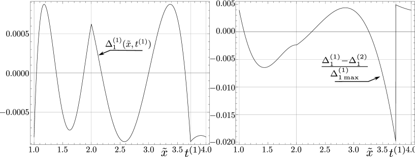
Figure 1: Left: graph of the function $\Delta_{1}^{(1)}(\tilde{x},t^{(1)})$. Right: $(\Delta_{1}^{(1)}(\tilde{x},t^{(1)})-\Delta_{1}^{(2)}(\tilde{x},t^{(2)}))$ as a fraction of $\Delta_{1\max}^{(1)}$.

Analogically we can determine the value of $d_{2}^{(1)}$ (assuming that $t=t^{(1)}$ is fixed):

$$-\frac{d_{2}^{(1)}-\max_{\tilde{x}\in\tilde{A}}|\Delta_{1}^{(1)2}(\tilde{x},t^{(1)})(3+\Delta_{1}^{(1)}(\tilde{x},t^{(1)}))|}{2-d_{2}^{(1)}}=\frac{d_{2}^{(1)}}{2-d_{2}^{(1)}}.$$ (5.12)

Now, the deepest minimum comes from the global maximum

$$\max_{\tilde{x}\in\tilde{A}}|\Delta_{1}^{(1)2}(\tilde{x},t^{(1)})(3+\Delta_{1}^{(1)}(\tilde{x},t^{(1)}))|=\frac{2\tilde{\delta}^{2}_{1\,\max}(3-\tilde{\delta}_{1\,\max})}{(2-\tilde{\delta}_{1\,\max})^{3}}.$$ (5.13)

Therefore we get

$$d_{2}^{(1)}=\frac{\tilde{\delta}^{2}_{1\,\max}(3-\tilde{\delta}_{1\,\max})}{(2-\tilde{\delta}_{1\,\max})^{3}}\simeq 1.15234\cdot 10^{-6},$$ (5.14)

and the maximum error of the second correction is given by

$$\Delta_{2\max}^{(1)}=\frac{d^{(1)}_{2}}{2-d_{2}^{(1)}}\simeq 5.76173\cdot 10^{-7}\simeq\frac{\tilde{\delta}_{2\,\max}}{7.98}.$$ (5.15)

The computer code for the algorithm described above is the following modification of $InvSqrt$:

1.	float InvSqrt1(float x){
2.		float simhalfnumber = 0.50043818f * x;
3.		int i = *(int*) &x;
4.		i = 0x5F375A86 - (i$>>$1);
5.		x = *(float*)&i;
6.		x = x*(1.5013145f - simhalfnumber*x*x);
7.		x = x*(1.5000008f - 0.99912498f*simhalfnumber*x*x);
8.		return x ;
9.	}

where

$$0.50043818f \simeq(2-d_{1}^{(1)})^{-1},\quad \quad 1.5013145f \simeq 3(2-d_{1}^{(1)})^{-1},$$

$$1.5000008f \simeq 3(2-d_{2}^{(1)})^{-1},\quad \quad 0.99912498f \simeq(2-d_{1}^{(1)})(2-d_{2}^{(1)})^{-1}.$$

Comparing $InvSqrt1$ with $InvSqrt$ we easily see that the number of algebraic operations in $InvSqrt1$ is greater just by 1 (an additional multiplication in line $7$, corresponding to the second iteration of the modified Newton-Raphson procedure).

6 Algorithm InvSqrt2

Approximating $1/\sqrt{\tilde{x}}$ by $\tilde{y}_{30}$ and $\tilde{y}_{31}$, respectively, we transfom (3.1) into

$$\begin{array}[]{l}\displaystyle\tilde{y}_{31}=\frac{1}{2}\tilde{y}_{30}(3-\tilde{y}_{30}^{2}\,\tilde{x})+\frac{1}{2}d_{1}\tilde{y}_{30},\\[7.74997pt] \displaystyle\tilde{y}_{32}=\frac{1}{2}\tilde{y}_{31}(3-\tilde{y}_{31}^{2}\,\tilde{x})+\frac{1}{2}d_{2}\tilde{y}_{31},\end{array}$$ (6.1)

where $\tilde{y}_{3k}$ ($k=1,2,\ldots$) depend on $\tilde{x},t$ and $d_{j}$ (for $j\leqslant k$). We assume $\tilde{y}_{30}\equiv\tilde{y}_{00}$. Thus $\tilde{y}_{31}$ and $\tilde{y}_{32}$ can be explicitly expressed by $\tilde{y}_{30}$ and $\tilde{y}_{31}$, respectively. The error functions are defined in the usual way:

$$\Delta_{k}^{(2)}=\sqrt{\tilde{x}}\,\tilde{y}_{3k}-1\ .$$ (6.2)

Substituting (6.2) into (6.1) we get:

$$\Delta_{1}^{(2)}(\tilde{x},t,d_{1})=\frac{1}{2}d_{1}\left(1+\tilde{\delta}_{0}(\tilde{x},t)\right)-\frac{1}{2}\tilde{\delta}_{0}^{2}(\tilde{x},t)\left(3+\tilde{\delta}_{0}(\tilde{x},t)\right)$$ (6.3)

$$\Delta_{2}^{(2)}(\tilde{x},t,d_{1},d_{2})=\frac{1}{2}d_{2}\left(1+{\Delta^{(2)}_{1}}\right)-\frac{1}{2}\left(\Delta_{1}^{(2)}\right)^{2}\left(3+\Delta_{1}^{(2)}\right),$$ (6.4)

where $\Delta_{1}^{(2)}\equiv\Delta_{1}^{(2)}(\tilde{x},t,d_{1})$.

First, we are going to determine $t$ and $d_{1}^{(2)}$ minimizing the maximum absolute value of the relative error of the first correction. Therefore, we have to solve the following equation:

$$0=\frac{\partial\Delta_{1}^{(2)}(\tilde{x},t)}{\partial\tilde{\delta}_{0}(\tilde{x},t)}=\frac{1}{2}d_{1}^{(2)}-3\tilde{\delta}_{0}(\tilde{x},t)-\frac{3}{2}\tilde{\delta}_{0}^{2}(\tilde{x},t).$$ (6.5)

Its solution

$$\tilde{\delta}^{+}=\sqrt{1+d_{1}^{(2)}/3}-1$$ (6.6)

corresponds to the value

$${\Delta}^{(2)}_{1\max}=\frac{1}{2}d_{1}^{(2)}(1+\tilde{\delta}^{+})-\frac{1}{2}\tilde{\delta}^{+2}(3+\tilde{\delta}^{+}),$$ (6.7)

which is a maximum of $\Delta_{1}^{(2)}(\tilde{x},t)$ because its second derivative with respect to $\tilde{x}$, i.e.,

$$\partial_{\tilde{x}}^{2}\Delta_{1}^{(2)}(\tilde{x},t)=\partial^{2}_{\tilde{x}}\tilde{\delta}_{0}(\tilde{x},t)\partial_{\tilde{\delta}_{0}}{\Delta}_{1}^{(2)}(\tilde{x},t)-3(1+\tilde{\delta}_{0}(\tilde{x},t))(\partial_{x}\tilde{\delta}_{0}(\tilde{x},t))^{2},$$ (6.8)

is negative. In order to determine the dependence of $d_{1}^{(2)}$ on the parameter $t$ we solve the equation

$$-\Delta_{1}^{(2)}(t,t)={\Delta}^{(2)}_{1\max},$$ (6.9)

which equates (for some $t=t^{(2)}$) the maximum value of error with the modulus of the minimum value of error. Thus we obtain the following relations:

$$\delta^{+} =-1-\frac{1}{4}\sqrt{t}+\frac{1}{8}\frac{t}{f(t)}+\frac{1}{2}f(t),$$ (6.10)

$$d_{1}^{(2)} =-3+\frac{9}{16}t+\frac{3}{64}t^{2}f^{-2}(t)-\frac{3}{16}t^{3/2}f^{-1}(t)-\frac{3}{4}\sqrt{t}f(t)+\frac{3}{4}f^{2}(t),$$ (6.11)

where

$$f(t)=\left[8+t^{3/2}/8+4\sqrt{4+t^{3/2}/8}\right]^{1/3}.$$

The next step consists in finding $t=t^{(2)}$ satisfying the condition analogical to (5.7), namely:

$$\forall_{t\neq t^{(2)}}\max_{\tilde{x}\in\tilde{A}}|{\Delta}_{1}^{(2)}(\tilde{x},t^{(2)})|\leq\max_{\tilde{x}\in\tilde{A}}|{\Delta}_{1}^{(2)}(\tilde{x},t)|.$$ (6.12)

For this purpose we solve numerically the equation

$$\Delta_{1}^{(2)}(t,t)=\frac{1}{2}d_{1}^{(2)}(1+\tilde{\delta}_{0}(\tilde{x}_{0}^{II},t))-\frac{1}{2}\tilde{\delta}_{0}^{2}(\tilde{x}_{0}^{II},t)(3+\tilde{\delta}_{0}(\tilde{x}_{0}^{II},t)),$$ (6.13)

which equates the minimum boundary value of the error of analysed correction with its smallest local minimum, where $x_{0}^{II}$ is given by (2.11). Thus we obtain $t^{(2)}$:

$$t^{(2)}\simeq 3.73157124016,$$ (6.14)

which is closer to $t_{0}^{(r)}$ than $t_{1}^{(r)}$. The value $t=t^{(2)}$ found in this way corresponds to the following magic constant:

$$\tilde{R}^{(2)}=1597466888=0x5F376908$$ (6.15)

and to the relative error

$$\Delta_{1\max}^{(2)}\simeq 8.7908386407\cdot 10^{-4}\simeq\frac{\tilde{\delta}_{1\max}}{1.99},\quad d_{1}^{(2)}=1.75791023259\cdot 10^{-3}.$$ (6.16)

In spite of the fact that this error is only slightly greater than $\Delta^{(1)}_{1\max}$,

$$\frac{\Delta^{(2)}_{1\max}-\Delta^{(1)}_{1\max}}{\Delta^{(1)}_{1\max}}\simeq 0.3\%,$$

the difference between error functions, i.e.,

$${\Delta_{1}^{(1)}(\tilde{x},t^{(2)})-\Delta_{1}^{(2)}(\tilde{x},t^{(1)})},$$

can reach much higher values, even $2\%$ of $\Delta_{1\max}^{(1)}$ (see Fig. 1), due to a different estimation of the parameter $t$.

In the case of the second correction, we keep the obtained value $t=t^{(2)}$ and determine the parameter $d_{2}^{(2)}$ equating the maximum value of the error with the modulus of its global minimum. ${\Delta^{(2)}_{2}}(\tilde{x},t^{(2)})$ is increasing (decreasing) with respect to negative (positive) ${\Delta^{(2)}_{1}}(\tilde{x},t^{(2)})$ and has local minima which come only from positive maxima and negative minima. Therefore the global minimum should correspond to the global minimum $-\Delta_{1\max}^{(2)}$ or to the global maximum $\Delta_{1\max}^{(2)}$. Substituting these values to Eq. (6.4) in the place of $\Delta_{1}^{(2)}(\tilde{x},t^{(2)})$ we obtain that deeper minima of $(-\Delta_{2\max}^{(2)})$ come from the global minimum of the first correction:

$$-\Delta_{2\max}^{(2)}=\frac{1}{2}d_{2}^{(2)}(1-\Delta_{1\max}^{(2)})-\frac{1}{2}\Delta_{1\max}^{(2)2}(3-\Delta_{1\max}^{(2)}),$$ (6.17)

and the maximum, by analogy to the first correction, corresponds to the following value of $\Delta_{1}^{(2)}(\tilde{x},t^{(2)})$:

$$\Delta^{+}=\sqrt{1+d_{2}^{(2)}/3}-1.$$ (6.18)

Solving the equation

$$\Delta_{2\max}^{(2)}=\frac{1}{2}d_{2}^{(2)}(1+\Delta^{+})-\frac{1}{2}\Delta^{+2}(3+\Delta^{+})$$ (6.19)

we get

$$d_{2}^{(2)}\simeq 1.159352515\cdot 10^{-6}\quad\text{and}\quad\Delta_{2\max}^{(2)}\simeq=5.796763137\cdot 10^{-7}\simeq\frac{\tilde{\delta}_{2\max}}{7.93}.$$ (6.20)

Thus we completed the derivation of the function $InvSqrt2$. The computer code contains a new magic constant, see (6.15), and has two lines ($6$ and $7$) modified as compared with the code $InvSqrt$:

1.	float InvSqrt2(float x){
2.		float halfnumber = 0.5f * x;
3.		int i = *(int*) &x;
4.		i = 0x5F376908 - (i$>>$1);
5.		x = *(float*)&i;
6.		x = x*(1.5008789f - halfnumber*x*x);
7.		x = x*(1.5000006f - halfnumber*x*x);
8.		return x ;
9.	}

where

$$1.5008789f\simeq\frac{3+d_{1}^{(2)}}{2},\quad\quad 1.5000006f\simeq\frac{3+d_{2}^{(2)}}{2}.$$

We point out that the code $InvSqrt2$ has the same number of algebraic operations as $InvSqrt$.

7 Numerical experiments

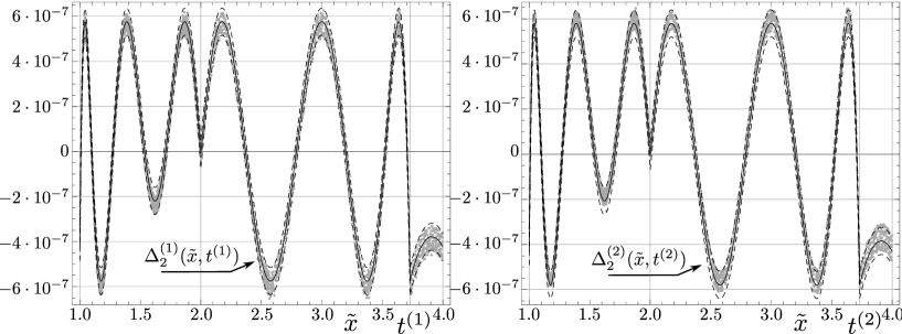
Figure 2: Solid lines represent functions $\Delta_{2}^{(1)}(\tilde{x},t^{(1)})$ (left) and $\Delta_{2}^{(2)}(\tilde{x},t^{(2)})$ (right). Their vertical shifts by $\pm 6\cdot 10^{-8}$ are denoted by dashed lines. Finally, dots represent relative errors for $4000$ random values $x\in(2^{-126},2^{128})$, produced by algorithms $InvSqrt1$ (left) and $InvSqrt2$ (right).

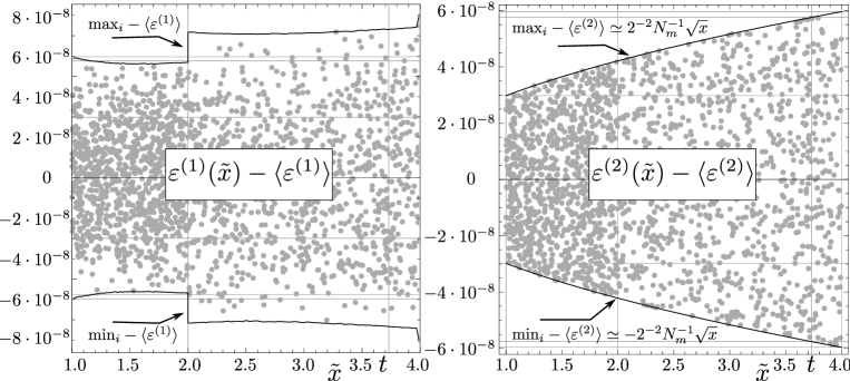
Figure 3: Relative errors $\varepsilon^{(1)}$ (left) and $\varepsilon^{(2)}$ (right) arising during the float approximation of corrections $\tilde{y}_{22}(\tilde{x},t)$ and $\tilde{y}_{32}(\tilde{x},t)$, respectively. Dots represent errors determined for $2000$ random values $\tilde{x}\in[1,4)$. Solid lines represent maximum ($\max_{i}$) and minimum ($\min_{i}$) values of relative errors (intervals $[1,2)$ and $[2,4)$ were divided into $64$ equal intervals, and then extremum values were determined in all these intervals).

The new algorithms were tested on the processor Intel Core 2 Quad (x86-64) using the compiler TDM-GCC 4.9.2 32-bit (then, in the case of $InvSqrt$, the values of erors are practically the same as those obtained by Lomont [24]). The same reults were obtained also on Intel i7-5700.

Applying the algorithm $InvSqrt1$ we obtain relative errors characterized by “oscillations” with a center slightly shifted with respect to the analytical solution, see Fig. 2. Although at figures we present only randomly chosen values but calculations were carried out for all numbers $x$ of the type float such that $e_{x}\in[-126,128)$, for any interval $A_{n}$ (see Eq. (2.7) in [45]). The range of errors is the same for all these intervals (except $e_{x}=-126$):

$$\Delta^{(1)}_{N}(x)=\mathrm{sqrt}(x)*\mathrm{InvSqrt1}(x)-1.\in(\Delta^{(1)}_{N,\min},\Delta^{(1)}_{N,\max}),$$ (7.1)

where

$$\Delta^{(1)}_{N,\min}=-6.62\cdot 10^{-7},\quad\quad\Delta^{(1)}_{N,\max}=6.35\cdot 10^{-7}.$$

For $e_{x}=-126$ the interval of errors is slightly wider:

$$[-6.72\cdot 10^{-7},6.49\cdot 10^{-7}].$$

The observed blur can be noticed already for the approximation error of the correction $\tilde{y}_{22}(\tilde{x})$:

$$\varepsilon^{(1)}(\tilde{x})=\frac{\mathrm{InvSqrt1(x)}-\tilde{y}_{22}(\tilde{x},t^{(1)})}{\tilde{y}_{22}(\tilde{x},t^{(1)})}.$$ (7.2)

The values of this error are distributed symmetrically around the mean value $\langle\varepsilon^{(1)}\rangle$:

$$\langle\varepsilon^{(1)}\rangle=2^{-1}N_{m}^{-23}\sum_{x\in[1,4)}\varepsilon^{(1)}(\tilde{x})=-1.398\cdot 10^{-8}$$ (7.3)

enclosing the range:

$$\varepsilon^{(1)}(\tilde{x})\in[-9.676\cdot 10^{-8},6.805\cdot 10^{-8}],$$ (7.4)

see Fig. 3. The blur parameters of the function $\varepsilon^{(1)}(\tilde{x},t)$ show that the main source of the difference between analytical and numerical results is the use of precision float and, in particular, rounding of constant parameters of the function $\mathrm{InvSqrt1(\tilde{x})}$. It is worthwhile to point out that in this case the amplitude of the error oscillations is about $40\%$ greater than the amplitude of oscillations of $(\tilde{y}_{00}-\tilde{y}_{0})/\tilde{y}_{0}$ (i.e., in the case of $InvSqrt$), see the right part of Fig. 2 in [45].

The errors of numerical values returned by $InvSqrt2$ belong (for $e_{x}\neq-126$) to the following interval

$$\Delta^{(2)}_{N}(x)=\mathrm{sqrt}(x)*\mathrm{InvSqrt2}(x)-1.\in(\Delta^{(2)}_{N,\min},\Delta^{(2)}_{N,\max}),$$ (7.5)

where

$$\Delta^{(2)}_{N,\min}=-6.21\cdot 10^{-7},\quad\quad\Delta^{(2)}_{N,\max}=6.53\cdot 10^{-7}.$$

For $e_{x}=-126$ we also get a wider interval:

$$[-6.46\cdot 10^{-7},6.84\cdot 10^{-7}].$$

These errors differ from the errors of $\tilde{y}_{32}(\tilde{x},t^{(2)})$ determined analytically (like in the case of the function $InvSqrt1$). The observed blur of the float approximation of the error of the correction $\tilde{y}_{32}(\tilde{x})$:

$$\varepsilon^{(2)}(\tilde{x})=\frac{\mathrm{InvSqrt2(x)}-\tilde{y}_{32}(\tilde{x},t^{(2)})}{\tilde{y}_{32}(\tilde{x},t^{(2)})},$$ (7.6)

is also symmetric with respect to the mean value $\langle\varepsilon^{(2)}\rangle$ (see Fig. 3):

$$\langle\varepsilon^{(2)}\rangle=2^{-1}N_{m}^{-23}\sum_{x\in[1,4)}\varepsilon^{(2)}(\tilde{x})=1.653\cdot 10^{-8}$$ (7.7)

but it covers a much smaller range of values:

$$\varepsilon^{(2)}(\tilde{x})\in[-4.316\cdot 10^{-8},7.612\cdot 10^{-8}]\;.$$ (7.8)

As a consequence, the maximum numerical error of the function $\mathrm{InvSqrt2}$ is smaller than the error of $\mathrm{InvSqrt1{}}$:

$$\max\{|\Delta_{N\min}^{(1)}|,\,|\Delta_{N\max}^{(1)}|\}=-\Delta_{N\min}^{(1)}>\Delta_{N\max}^{(2)}=\max\{|\Delta_{N\min}^{(2)}|,\,|\Delta_{N\max}^{(2)}|\}.$$ (7.9)

Results produced by the same hardware with 64-bit compiler have the amplitude of the error oscillations greater by about $10^{-7}$ as compared with the 32-bit case.

If we stop both algorithms after the first correction, then the numerical errors of $\mathrm{InvSqrt2}$ are contained in the interval

$$[-8.79\cdot 10^{-4},\,8.79\cdot 10^{-4}]\,,$$

which is a little bit wider than the analogical interval for $\mathrm{InvSqrt1}$

$$[-8.76\cdot 10^{-4},\,8.76\cdot 10^{-4}]\,.$$

Therefore, the code $\mathrm{InvSqrt1}$ is slightly more accurate than $\mathrm{InvSqrt2}$ as far as one iteration is concerned and both are about 2 times more accurate than $\mathrm{InvSqrt}$. Comparing $\Delta^{(2)}_{N,\max}$ with the analogical numerical bound for $\mathrm{InvSqrt}$ (see Eq. (4.23) in [45]) we conclude that in the case of two iterations the code $\mathrm{InvSqrt2}$ is about $7$ times more accurate than $\mathrm{InvSqrt}$. We point out that round-off errors significantly decrease the theoretical improvement which is given by the factor $8$.

8 Conclusions

In this paper we have presented two modifications of the famous InvSqrt code for fast computation of the inverse square root. The first modification, denoted by InvSqrt1, has the same magic constant as InvSqrt (i.e., the same initial values for the iteration process) but instead of the standard Newton-Raphson method we propose a similar procedure but with different coefficients. The obtained algorithm is slightly more expensive in the case of two iterations (8 multiplications instead of 7 at every step) but much more accurate than $InvSqrt$: two times more accurate after the first iteration and about 7 times more accurate after two iterations. The second modification, denoted by InvSqrt2, uses another magic constant. Its computational cost is practically the same as the cost of the InvSqrt code (both have the same number of multiplications). This is the main advantage of InvSqrt2 over InvSqrt1 because the accuracy of InvSqrt2 is similar to the accuracy of InvSqrt1. Analytical values for InvSqrt1 are slightly better but numerical tests show that round-off errors are a little bit greater in this case, see (7.1) and (7.5), although the situation becomes reversed when the algorithms are stopped after only one iteration.

Concerning potential applications, we have to acknowlede that for general purpose computing the SSE reciprocal square root instruction is faster and more accurate. We hope, however, that the proposed algorithms can be applied in embedded systems and microcontrollers that lack a FPU, and potentially in FPGA’s.

References

• [1] M.D. Ercegovac, T. Lang: Digital Arithmetic, Morgan Kaufmann 2003.
• [2] B. Parhami: Computer Arithmetic: Algorithms and Hardware Designs, $2^{nd}$ edition, Oxford Univ. Press, New York, 2010.
• [3] K. Diefendorff, P. K. Dubey, R. Hochsprung, H. Scales: AltiVec extension to PowerPC accelerates media processing, IEEE Micro 20 (2) (2000) 85-95.
• [4] D. Harris: A Powering Unit for an OpenGL Lighting Engine, Proc. 35th Asilomar Conf. Singals, Systems, and Computers (2001), pp. 1641-1645.
• [5] M. Sadeghian, J. Stine: Optimized Low-Power Elementary Function Approximation for Chybyshev series Approximation, 46th Asilomar Conf. on Signal Systems and Computers, 2012.
• [6] D. M. Russinoff: A Mechanically Checked Proof of Correctness of the AMD K5 Floating Point Square Root Microcode, Formal Methods in System Design 14 (1) (1999) 75-125.
• [7] M.Cornea, C. Anderson, C. Tsen: Software Implementation of the IEEE 754R Decimal Floating-Point Arithmetic, Software and Data Technologies (Communications in Computer and Information Science, vol. 10), Springer 2008, pp. 97-109.
• [8] J.-M. Muller, N. Brisebarre, F. Dinechin, C.-P. Jeannerod, V. Lefèvre, G. Melquiond, N. Revol, D.Stehlé, S. Torres: Hardware Implementation of Floating-Point Arithmetic, Handbook of Floating-Point Arithmetic (2009), pp. 269-320.
• [9] J.-M. Muller, N. Brisebarre, F. Dinechin, C.-P. Jeannerod, V. Lefèvre, G. Melquiond, N. Revol, D.Stehlé, S. Torres: Software Implementation of Floating-Point Arithmetic, Handbook of Floating-Point Arithmetic (2009), pp. 321-372.
• [10] T. Viitanen, P. Jääskeläinen, O. Esko, J. Takala: Simplified floating-point division and square root, Proc. IEEE Int. Conf. Acoustics Speech and Signal Process., pp. 2707–2711, May 26–31 2013.
• [11] M.D. Ercegovac, T. Lang: Division and Square Root: Digit Recurrence Algorithms and Implementations, Boston: Kluwer Academic Publishers, 1994.
• [12] T.J. Kwon, J. Draper: Floating-point Division and Square root Implementation using a Taylor-Series Expansion Algorithm with Reduced Look-Up Table, 51st Midwest Symposium on Circuits and Systems, 2008.
• [13] T.O. Hands, I. Griffiths, D.A. Marshall, G. Douglas: The fast inverse square root in scientific computing, Journal of Physics Special Topics 10 (1) (2011) A2-1.
• [14] W. Liu, A. Nannarelli: Power Efficient Division and Square root Unit, IEEE Trans. Comp. 61 (8) (2012) 1059-1070.
• [15] L.X. Deng, J.S. An: A low latency High-throughput Elementary Function Generator based on Enhanced double rotation CORDIC, IEEE Symposium on Computer Applications and Communications (SCAC), 2014.
• [16] M. X. Nguyen, A. Dinh-Duc: Hardware-Based Algorithm for Sine and Cosine Computations using Fixed Point Processor, 11th International Conf. on Electrical Engineering/Electronics Computer, Telecommuncations and Information Technology, IEEE 2014.
• [17] M. Cornea, Intel${}^{\textsuperscript{\textregistered}}$ AVX-512 Instructions and Their Use in the Implementation of Math Functions, Intel Corporation 2015.
• [18] H. Jiang, S. Graillat, R. Barrio, C. Yang: Accurate, validated and fast evaluation of elementary symmetric functions and its application, Appl. Math. Computation 273 (2016) 1160–1178.
• [19] A. Fog, Software optimization resources, Instruction tables: Lists of instruction latencies, throughputs and micro-operation breakdowns for Intel, AMD and VIA CPUs, http://www.agner.org/optimize/
• [20] D.H. Eberly: GPGPU Programming for Games and Science, CRC Press 2015.
• [21] N. Ide, M. Hirano, Y. Endo, S. Yoshioka, H. Murakami, A. Kunimatsu, T. Sato, T. Kamei, T. Okada, M. Suzuoki: 2.44-GFLOPS 300-MHz Floating-Point Vector-Processing Unit for High-Performance 3D Graphics Computing, IEEE J. Solid-State Circuits 35 (7) (2000) 1025-1033.
• [22] S. Oberman, G. Favor, F. Weber: AMD 3DNow! technology: architecture and implementations, IEEE Micro 19 (2) (1999) 37-48.
• [23] id software, quake3-1.32b/code/game/q_math.c , Quake III Arena, 1999.
• [24] C. Lomont, Fast inverse square root, Purdue University, Tech. Rep., 2003. Available online: http://www.matrix67.com/data/InvSqrt.pdf, http://www.lomont.org/Math/Papers/2003/InvSqrt.pdf.
• [25] H.S. Warren: Hacker’s delight, second edition, Pearson Education 2013.
• [26] P. Martin: Eight Rooty Pieces, Overload Journal 135 (2016) 8–12.
• [27] J. Blinn, Floating-point tricks, IEEE Comput. Graphics Appl. 17 (4) (1997) 80-84.
• [28] J. Janhunen: Programmable MIMO detectors, PhD thesis, University of Oulu, Tampere 2011.
• [29] J.L.V.M. Stanislaus, T. Mohsenin: High Performance Compressive Sensing Reconstruction Hardware with QRD Process, IEEE International Symposium on Circuits and Systems (ISCAS’12), May 2012.
• [30] Q. Avril, V. Gouranton, B. Arnaldi: Fast Collision Culling in Large-Scale Environments Using GPU Mapping Function, ACM Eurographics Parallel Graphics and Visualization, Cagliari, Italy (2012).
• [31] R. Schattschneider: Accurate high-resolution 3D surface reconstruction and localisation using a wide-angle flat port underwater stereo camera, PhD thesis, University of Canterbury, Christchurch, New Zealand, 2014.
• [32] S. Zafar, R. Adapa: Hardware architecture design and mapping of “Fast Inverse Square Root’s algorithm”, International Conference on Advances in Electrical Engineering (ICAEE), 2014, pp. 1-4.
• [33] T. Hänninen, J. Janhunen, M. Juntti: Novel detector implementations for 3G LTE downlink and uplink, Analog. Integr. Circ. Sig. Process. 78 (2014) 645- 655.
• [34] Z.Q. Li, Y. Chen, X.Y. Zeng: OFDM Synchronization implementation based on Chisel platform for 5G research, 2015 IEEE 11th International Conference on ASIC (ASICON).
• [35] C.J. Hsu, J.L. Chen, L.G. Chen: An Efficient Hardware Implementation of HON4D Feature Extraction for Real-time Action Recognition, 2015 IEEE International Symposium on Consumer Electronics (ISCE).
• [36] C.H. Hsieh, Y.F. Chiu, Y.H. Shen, T.S. Chu, Y.H. Huang: A UWB Radar Signal Processing Platform for Real-Time Human Respiratory Feature Extraction Based on Four-Segment Linear Waveform Model, IEEE Trans. Biomed. Circ. Syst. 10 (1) (2016) 219–230.
• [37] J.D. Lv, F. Wang, Z.H. Ma: Peach Fruit Recognition Method under Natural Environment, Eighth International Conference on Digital Image Processing (ICDIP 2016), Proc. of SPIE Vol. 10033, edited by C.M.Falco, X.D.Jiang, 1003317 (29 August 2016).
• [38] D. Sangeetha, P. Deepa: Efficient Scale Invariant Human Detection using Histogram of Oriented Gradients for IoT Services, 2017 30th International Conference on VLSI Design and 2017 16th International Conference on Embedded Systems, p. 61–66, IEEE 2016.
• [39] J. Lin, Z.G. Xu, A. Nukada, N. Maruyama, S. Matsuoka: Optimizations of Two Compute-bound Scientific Kernels on the SW26010 Many-core Processor, 46th International Conference on Parallel Processing, p. 432–441, IEEE 2017.
• [40] C. McEniry: The Mathematics Behind the Fast Inverse Square Root Function Code, Tech. rep. 2007.
• [41] M. Robertson: A Brief History of InvSqrt, Bachelor Thesis, Univ. of New Brunswick 2012.
• [42] B. Self: Efficiently Computing the Inverse Square Root Using Integer Operations. May 31, 2012.
• [43] D. Eberly: An approximation for the Inverse Square Root Function, 2015, http://www.geometrictools.com/Documentation/ApproxInvSqrt.pdf.
• [44] P. Kornerup, J.-M. Muller: Choosing starting values for certain Newton Raphson iterations, Theor. Comp. Sci. 351 (2006) 101 110.
• [45] L. Moroz, C.J. Walczyk, A. Hrynchyshyn, V. Holimath, J.L. Cieśliński: Fast calculation of inverse square root with the use of magic constant – analytical approach, Appl. Math. Computation 316 (2018) 245–255.
• [46] A. Ziv: Fast evaluation of elementary mathematical functions with correctly rounded last bit, ACM Trans. Math. Software 17 (3) (1991) 410–423.
• [47] F. De Dinechin, C. Lauter, J.-M. Muller, S. Torres: On Ziv’s rounding test, ACM Trans. Math. Software 39 (4) (2013) 25.