Resonance line broadened quasilinear (RBQ) model for fast ion distribution relaxation due to Alfvénic eigenmodes

Abstract

The burning plasma performance is limited by the confinement of the superalfvenic fusion products such as alpha particles and the auxiliary heating ions capable of exciting the Alfvénic eigenmodes (AEs) Gorelenkov et al. (2014). In this work the effect of AEs on fast ions is formulated within the quasi-linear (QL) theory generalized for this problem recently Duarte (2017). The generalization involves the resonance line broadened interaction of energetic particles (EP) with AEs supplemented by the diffusion coefficients depending on EP position in the velocity space. A new resonance broadened QL code (or RBQ1D) based on this formulation allowing for EP diffusion in radial direction is built and presented in details. We reduce the wave particle interaction (WPI) dynamics to 1D case when the particle kinetic energy is nearly constant. The diffusion equation for EP distribution evolution is then one dimensional and is solved simultaneously for all particles with the equation for the evolution of the wave angular momentum. The evolution of fast ion constants of motion is governed by the QL diffusion equations which are adapted to find the fast ion distribution function.

We make initial applications of the RBQ1D to DIII-D plasma with elevated $q$-profile where the beam ions show stiff transport properties Collins et al. (2016). AE driven fast ion profile relaxation is studied for validations of the QL approach in realistic conditions of beam ion driven instabilities in DIII-D.

I Introduction

Despite the significant progress in the modeling of energetic particle (EP) driven instabiliteis in tokamaks in recent years, we still lack the reliable quantitative and predictive capabilities for fast ion confinement Heidbrink et al. (2008); Gorelenkov et al. (2014). When the dominant mechanism for fast ion transport is diffusive, a promising reduced approach is the quasi-linear (QL) modeling which offers the advantage of a simplified, and therefore less computationally demanding framework Drummond and Pines (1962); Vedenov et al. (1961). If the mediator of EP transport is a collective instability such as the Alfvénic eigenmode (AE) instability, the eigenmode structure and resonances is assumed to be fixed in time. Thus the modes can be treated perturbatively while the distribution function is allowed to evolve. For this reason the standard QL approach does not capture the instability frequency chirping or avalanches which are common Alfvénic spectral response that consist of fully nonlinear oscillations. We should note that a criterion for the likelihood of wave chirping onset (alternatively, a criterion for the non-applicability of the QL approach) has been recently derived and validated Duarte et al. (2017a, b), which verifies the application of the QL approach for practical cases.

While the conventional QL theory Drummond and Pines (1962); Vedenov et al. (1961); Kaufman (1972) only applies to the situations with multiple modes overlapping (i.e., when the Chirikov criterion Chirikov (1960) of resonance overlapping is satisfied), a line broadened quasilinear model Berk et al. (1995, 1996a) was designed to address the particle interaction with both isolated and overlapping modes. This is done by using the same structure of QL equations for fast ion distribution function (DF) but with the diffusive delta function broadened along the relevant path of resonant particles to produce a resonance line broadened quasilinear (RBQ) diffusion. This is a key element of the RBQ model that the parametric dependencies of the broadened window reproduce the expected saturation levels for isolated modes. An important factor of RBQ applicability is the presence of the velocity space diffusion Meng et al. (2018) which partially includes the convective transport through the radial dependence of the diffusion coefficient.

The system of equations we use in the RBQ code was initially implemented for the case of the bump-on-tail configuration in Fitzpatrick’s thesis Fitzpatrick (1997). Ghantous Ghantous et al. (2014a); Ghantous (2013) benchmarked this model with the Vlasov code bump-on-tail (BOT) discussing regimes of its applicability. We revisit the RBQ model and modify it to the realistic cases of Alfvénic instabilities excited by the super-Alfvénic energetic ions for the first time. We express the RBQ equations in action and angle variables, and implement them within the NOVA/NOVA-K framework for subsequent TRANSP code simulations. Results are presented for DIII-D discharge with the reversed shear safety factor profile and with elevated $q_{min}$ values described recently Collins et al. (2016); Heidbrink et al. (2017). We show the predictive capability of the RBQ model and compare it with the results of the the kick model Podestà et al. (2014, 2017).

This paper is organized as follows. The introduction is given in section I. Then in section II we start the description of the RBQ formulation by prescribing the resonance line broadening in the Constants of Motion (COM) space to account for fast ion dynamics near the resonances. Section III presents the RBQ system of differential equations written in flux and COM variables. Section IV describes the adopted Probability Density Function (PDF) interface with the Whole Device Modeling (WDM) prototype code TRANSP Goldston et al. (1981). Then Sec. V presents the RBQ results for selected DIII-D discharge. Finally section VI summarizes the study and outlines future RBQ development.

II Generalized Resonance Broadening Framework

We introduce the QL model by describing first the resonance line broadening which we make use of when building the RBQ code.

II.1 Resonance broadening and its parametric dependencies

Consider the wave particle interaction (WPI) resonance line broadening in two-dimensional space Dupree (1966) to investigate the problem of EP transport in the presence of realistic Alfvén eigenmodes. The QL diffusion of a particle is along the paths of constant values of the expression

$$\omega P_{\varphi}+n\mathcal{E}=n\mathcal{E}^{\prime}=const,$$ (1)

where $\omega$ and $n$ are the angular frequency and toroidal mode number of the instability. If the diffusion is approximately along $P_{\varphi}$, i.e. at the low mode frequency the whole problem can be reduced to the set of 1D ($\Delta\mathcal{E}\simeq 0$) equations as discussed in Fitzpatrick’s thesis Fitzpatrick (1997). An appropriate rotation in space reduces the diffusion equations of the RBQ model to the set of one-dimensional equations that are straightforward to solve. The effect of several low-$n$ modes on energetic particles cannot be determined without the code that captures the diffusion in full $\mathcal{E},P_{\varphi}$ space. This is due to the complex particle dynamics in 2D space and possible resonance overlap White et al. (2010).

The conventional collisionless QL diffusion set of equations in terms of action and angle variables can be expressed as Kaufman (1972)

$$\frac{\partial}{\partial t}f\left({\bf J};t\right)=\frac{\partial}{\partial{\bf J}}\left[\underline{\underline{D}}(\mathbf{J};t)\frac{\partial f}{\partial{\bf J}}\right],$$ (2)

$$\underline{\underline{D}}(\mathbf{J};t)=\frac{2\pi}{M^{2}}\underset{k}{\sum}\frac{C_{k}^{2}\left(t\right)}{\omega_{k}^{2}}\underset{{\bf l}}{\sum}{\bf l}{\bf l}\delta\left({\bf l}\cdot\bm{\omega_{AI}}\left({\bf J}\right)-\omega_{k}\right)\alpha_{{\bf l}}^{k}\left({\bf J}\right),$$ (3)

$$\frac{dC_{k}^{2}(t)}{dt}=2\left(\gamma_{L,k}-\gamma_{d,k}\right)C_{k}^{2}(t),$$ (4)

$$\gamma_{L,k}=\frac{\left(2\pi\right)^{3}}{\omega_{k}M\delta K}\int d{\bf J}\underset{{\bf l}}{\sum}\alpha_{{\bf l}}^{k}\left({\bf J}\right)\left({\bf l}\cdot\frac{\partial f}{\partial{\bf J}}\right)\pi\delta\left({\bf l}\cdot\bm{\omega_{AI}}\left({\bf J}\right)-\omega_{k}\right),$$ (5)

with index $k$ denoting the mode of interest and structure contributions (often called matrix elements) are given by

$$\alpha_{{\bf l}}^{k}\left({\bf J}\right)\equiv\left|\int d{\bf x}\mathbf{e}_{k}\left(\mathbf{x},\omega_{k}\right)\cdot{\bf j_{l}}^{k}\left({\bf x}\mid{\bf J}\right)\right|^{2},$$

where $M$ is the resonant particle mass, ${\bf J}=\left(J_{1},,J_{2},,J_{3}\right)$ is the vector of actions of EP unperturbed motion (they can be substituted by COMs in NOVA notations $\mathcal{E},P_{\varphi},\mu$), $f$ is the EP distribution function, $\underline{\underline{D}}$ is EP diffusion coefficient matrix. $\omega_{k}$, $C_{k}$ and $\mathbf{e}_{k}$ are the eigenmode frequency, mode amplitude and the electric field structure. $\bm{\omega_{AI}}\equiv\left(\omega_{A1},\omega_{A2},\omega_{A3}\right)$ is the canonical (action related) frequency vector containing the frequencies associated with the canonical angles and $\bm{l}=\left(l_{1},l_{2},l_{3}\right)$ is the vector of integer triad, $\gamma_{L,k}$ is the linear growth of the mode, $\gamma_{d,k}$ is the wave damping rate in the absence of the instability, $\omega_{k}\delta K$ is the mode wave energy normalized by $C_{k}^{2}$ and ${\bf j_{l}}^{k}\left({\bf x}\mid{\bf J}\right)$ means the resonant particle current at radial point ${\bf x}$ and having an action ${\bf J}$ (given in Appendix A), and the index $k$ relates the quantity to the $k$-th mode. The resonance condition is represented by $\omega_{k}-{\bf l}\cdot\bm{\omega_{AI}}\left({\bf J}\right)=0$. In the following we will use the resonance frequency notation:

$$\Omega\left({\bf J}\right)\equiv{\bf l}\cdot\bm{\omega_{AI}}\left({\bf J}\right).$$ (6)

The QL theory assumes that the mode amplitudes remain small and therefore the theoretical coefficients are computed based on the unperturbed orbits. In conventional QL theory, particles are considered to be in resonance only if they exactly satisfy the wave resonance condition. This implies that resonant particles can only diffuse over the resonant point, which is clearly an ill-posed problem. Nonlinear effects, however, naturally broaden the resonances. Dupree Dupree (1966) realized that the turbulent spectrum contributes to diffuse particle orbits away from their original unperturbed trajectories. In the RBQ model the resonant island width is incorporated into the QL theory in such a way that it reproduces the expected saturation levels for single modes from analytic theory Berk and Breizman (1990a). The broadening itself introduces an additional nonlinearity into the problem. The resonance line is substituted by the broadening function $\mathcal{F}$ to replace the resonance delta function. The broadening function becomes a more realistic platform that allows the momentum and energy exchange between particles and waves Meng et al. (2018).

In the RBQ model the window width is determined by the sum of three terms:

1. The net growth rate ($\gamma_{k}\equiv\gamma_{L,k}+\gamma_{d,k}$, where $\gamma_{L,k}$ and $\gamma_{d,k}$ are the linear (positive) growth and (negative) damping rates) as expected for the wave treated by ordinary quasilinear theory. As long as the imaginary part of the frequency is accounted for, the diffusion coefficient naturally contains the Lorentzian (Cauchy) distribution which has the property of having the characteristic height of $1/\gamma_{k}$ and the full width equal to $2\gamma_{k}$ at half maximum. The broadening is based on $\gamma_{k}$ and collapses to a delta function when $\gamma_{k}\rightarrow 0$, i.e. when the mode reaches saturation:

   $$\pi\delta\left(\Omega\left({\bf J}\right)-\omega_{k}\right)\underset{\gamma_{k}\neq 0}{\rightarrow}\frac{\gamma_{k}}{\left(\Omega\left({\bf J}\right)-Re\left\{\omega_{k}\right\}\right)^{2}+\gamma_{k}^{2}}.$$

2. The separatrix width expected for the wave treated by single mode theory. In the phase space, particles that exchange energy with the mode are trapped by the separatrix of width $4\omega_{b,k}$ Meng et al. (2018). Each particle satisfy a nonlinear pendulum equation with the given bounce trapping frequency $\omega_{b,k}$ which leads to the phase mixing for a single wave.

3. The effective collisional frequency $\nu_{scatt,k}$ (as defined in Berk et al. (1997); Gorelenkov et al. (1999a)) since collisions imply that particles are redistributed, being kicked in and out of the separatrix, which leads to particle decorrelating from the resonance. This increases the effective range of the resonance region since more particles are allowed to interact with the mode via the resonant platform. The presence of collisions actually simplifies the QL theory as it allows for phase information decorrelation which gives the delta functions a broadened width. The value of $\nu_{scatt,k}$ is sensitive to the choice of the mode numbers and frequency.

It has been found Fitzpatrick (1997); Ghantous et al. (2014b) that

$$\triangle\Omega_{k}\left(\mathcal{E},P_{\varphi},\mu\right)=a\omega_{b,k}+b\left|\gamma_{k}\right|\left\{=\left|\gamma_{L,k}+\gamma_{d,k}\right|\right\}+c\nu_{scatt,k},$$ (7)

where the other two frequencies can be expressed as follows Gorelenkov et al. (1999a):

$$\nu_{scatt,k}^{3}\simeq\nu_{\perp}R^{2}\left\langle v^{2}-v_{\|}^{2}\right\rangle\left(\left.\frac{\partial\Omega}{\partial P_{\varphi}}\right|_{\mathcal{E}\text{'}}\right)^{2},$$ (8)

$\nu_{\perp}$ is the $90^{0}$ pitch-angle scattering rate, $\left\langle\right\rangle$ is the drift orbit average, and

$$\omega_{b,k}=\left|2C_{k}(t)V_{k}(I_{r})\left.\frac{\partial\Omega}{\partial I}\right|_{I=I_{r}}\right|^{1/2},$$ (9)

where the subscript $r$ denotes the resonant location in the phase space. The numerical constants $a$ and $c$ are chosen to best fit the analytic theory.

III RBQ System of Equations

For the single mode WPI case, the particle diffusion can be projected onto the most relevant 1D path for EP dynamics in the phase space which occurs for the constant values of the magnetic moment $\mu$ and $\mathcal{E}^{\prime}$. Thus it is convenient to define the following differential operator that is essentially a gradient operator projected onto this path:

$$\frac{\partial}{\partial I}=\omega_{k}\frac{\partial}{\partial\mathcal{E}}-n\frac{\partial}{\partial P_{\varphi}}=\left.\omega_{k}\frac{\partial}{\partial\mathcal{E}}\right|_{P^{\prime}_{\varphi}}=\left.-n\frac{\partial}{\partial P_{\varphi}}\right|_{\mathcal{E}^{\prime}}.$$ (10)

Then, the 1D RBQ equation for a single mode written is

$$\frac{\partial f}{\partial t}=\frac{\partial}{\partial I}\left(\sum_{k,l,m,m^{\prime}}D(I;t)\right)\frac{\partial}{\partial I}f+\left(\left|\frac{\partial\Omega_{l}}{\partial I}\right|_{I_{r}}\right)^{-2}\nu_{scatt}^{3}\frac{\partial^{2}(f-f_{0})}{\partial I^{2}},$$ (11)

where

$$D(I;t)=\pi n_{k}^{2}C_{k}^{2}\left(t\right)\mathcal{E}^{2}\frac{\mathcal{F}\left(I-I_{r}\right)}{\left|\frac{\partial\Omega_{l}}{\partial I}\right|}G_{m^{\prime}l}^{*}G_{ml},$$ (12)

and the matrixes $G$ are defined in Appendix A.

The growth rate is given by (cf. Appendix A)

$$\gamma_{L,k}=\frac{2M^{2}\pi^{3}c}{z\omega_{k}\int\rho\left|\bm{\xi}\right|^{2}d{\bf r}}\underset{\sigma_{\parallel}}{\sum}\int dP_{\varphi}d\mu d\mathcal{E}\sum_{m,m^{\prime},l}G_{m^{\prime}l}^{*}\mathcal{E}^{2}\tau_{b}\frac{\partial}{\partial I}fG_{ml}\frac{\mathcal{F}\left(I-I_{r}\right)}{\left|\partial\Omega_{l}/\partial I\right|},$$ (13)

where $z$ is the EP electric charge, and $\tau_{b}$ is the drift orbit period. The full system of RBQ equations is comprised by (11), (4), (13) and (7).

The resonances are given by (cf. Eq.(6))

$$\Omega_{l}\left(\mathcal{E},P_{\varphi},\mu\right)=n_{k}\left\langle\omega_{\varphi}\left(\mathcal{E},P_{\varphi},\mu\right)\right\rangle-l\left\langle\omega_{\theta}\left(\mathcal{E},P_{\varphi},\mu\right)\right\rangle=\omega_{k}$$

where $l$ is an integer, $\omega_{\varphi}\equiv\dot{\varphi}$ and $\omega_{\theta}\equiv\dot{\theta}$ are the toroidal and poloidal precession frequency contributions. Note that $\Omega_{l}$ definition of our paper is not sensitive to the properties of each $k$-th mode but only to its toroidal mode number.

The derivatives $\partial\Omega_{l}/\partial I$ are provided by NOVA-K. The broadening of the resonance can be performed by choosing $\mathcal{F}$ as the window function with the width $\triangle I$ that satisfies $\int_{-\infty}^{\infty}\mathcal{F}dI=1$. The function $\mathcal{F}$ can be arbitrarily chosen. It can, for example, be a flat top, a Gaussian shaped or perhaps even specified via the Dupree’s window shape Dupree (1966), which for the BOT case can be transformed to 1D window function across the resonance

$$\mathcal{F}_{Dupree}=Re\int_{0}^{\infty}dt\exp\left[i\left(\Omega_{l}-\omega_{k}\right)t-D\left(\frac{\partial\Omega_{l}}{\partial I}\right)^{2}t^{3}/3\right].$$ (14)

III.1 Discretized equations and boundary conditions

Although in principle one can arbitrarily discretize the system of equations to solve them numerically, there are some restrictions that are implied by physical considerations. In order to conserve the system momentum (i.e., particle plus wave momenta) at all times, the discretized equations must guarantee internal self-consistency by adopting the time flow presented in Duarte (2017). This flow is chosen in such a way that both particle diffusion and mode amplitude evolution are calculated using the same window function at each time step.

The linear system matrix can only be inverted (and therefore the system can only be solved) when boundary conditions are added to the discretized system of equations. The code needs to account for a loss boundary in $\mathcal{E},P_{\varphi}$ plane that is different for each $\mu=const$ slice. A Neumann-type condition specifies the values that the derivative of the distribution function takes at the boundaries of the domain. It imposes a constant flux $\Gamma=-D\partial f/\partial I$ at the edge. Normally in the steady state this is associated with the reflective boundary conditions, when $D\partial f/\partial I=0$. On the other hand, the Dirichlet-type boundary condition imposes a constraint on the value of the function itself, such as at the loss cone when its value is mediated by the diffusion when we set up $f=0$.

In our diffusion solver to relax the EP distribution function, we have the option to use either Neumann or Dirichlet boundary conditions. They are chosen based on the following physical arguments. At the loss boundary, $f$ should be zero and Dirichlet is physically appropriate since it allows for particle loss. On the other hand for the inner regions of the plasma the resonant particles are allowed to accumulate and a Neumann condition describes the relevant physics (it is equivalent to a reflective condition, i.e., with zero net flux). Particle number over the plasma volume is automatically preserved if particles do not escape at the ends. However if particles reach the ends where they are unconfined the particle loss is quantifiable.

IV Probability Density Function Interface with Whole Device Modeling

We integrate the RBQ simulations in its present version into the transport code TRANSP which can be viewed as a prototype of the WDM code. It enables the time-dependent integrated simulations of a tokamak discharge. The code can be used to interpret existing experiments as well as to develop new scenarios or make predictions for future devices (e.g. ITER). For NB-heated discharges the NUBEAM module within TRANSP models the evolution of the energetic particle population based on neoclassical physics Goldston et al. (1981); Pankin et al. (2004). Coulomb collisions, slowing down and charge-exchange events are modeled based on a Monte Carlo approach. To account for resonant fast ion transport induced by Alfvénic and other MHD instabilities, NUBEAM has been updated to include the physics-based reduced model, known as kick model Podestà et al. (2014, 2017).

For NUBEAM calculations the kick model prepares the transport probability matrix, $p(\Delta\mathcal{E},\Delta P_{\varphi}|\mathcal{E},P_{\varphi},\mu)$, for each instability or a set of instabilities to be included in simulations. The matrix is defined in COM variables. For each COM grid point (or bin) in the phase space, $p(\Delta\mathcal{E},\Delta P_{\varphi})$ represents the probability of $\mathcal{E}$ and $P_{\varphi}$ changes (kicks) experienced by the energetic ions as a result of their interaction with the instability.

In previous works Podestà et al. (2016a, b, 2017) the transport probability matrices were computed numerically by the guiding center code ORBIT White and Chance (1984) using the mode structures from the NOVA code (details on how the matrix is computed for a given instability are found in the Appendix of Ref.Podestà et al. (2017)). In this work the quasi-linear diffusion coefficient computed by the RBQ1D code is used instead to reconstruct the $p(\Delta\mathcal{E},\Delta P_{\varphi}|\mathcal{E},P_{\varphi},\mu)$ probabilities under the assumption of negligible energy variations induced by the wave-particle interactions.

Consider the trajectory of a resonant particle subject to constraints in the $(\mathcal{E},P_{\varphi},\mu)$ space White (2011, 2012): Equation (1) implies that for a single mode the variations in $\mathcal{E}$ and $P_{\varphi}$ are related through

$$\Delta P_{\varphi}/\Delta\mathcal{E}=n/\omega.$$ (15)

Based on this constraint and under the assumption of diffusive transport (implied by the RBQ1D formulation), the bi-variate PDF for $\Delta\mathcal{E}$ and $\Delta P_{\varphi}$ changes can be represented as:

$$p\left(\Delta\mathcal{E},\Delta P_{\varphi}|P_{\varphi},\mathcal{E},\mu,A_{kick}\right)=p_{0}e^{-\left[\frac{\left(\Delta\mathcal{E}-\Delta\mathcal{E}_{0}\right)^{2}}{\sigma_{\mathcal{E}}^{2}}+\frac{\left(\Delta P_{\varphi}-\Delta P_{\varphi 0}\right)^{2}}{\sigma_{P_{\varphi}}^{2}}-2\rho\frac{(\Delta\mathcal{E}-\Delta\mathcal{E}_{0})(\Delta P_{\varphi}-\Delta P_{\varphi 0})}{\sigma_{\mathcal{E}}\sigma_{P_{\varphi}}}\right]/2\left(1-\rho\right)},$$ (16)

with the normalization factor

$$p_{0}=\frac{1}{2\pi\sigma_{\mathcal{E}}\sigma_{P_{\varphi}}\sqrt{1-\rho^{2}}}.$$ (17)

The correlation parameter $\rho=\frac{\left\langle\left(\Delta\mathcal{E}-\Delta\mathcal{E}_{0}\right)\left(\Delta P_{\varphi}-\Delta P_{\varphi 0}\right)\right\rangle}{\sigma_{\mathcal{E}}\,\sigma_{P_{\varphi}}}$ takes into account coupling between $\Delta\mathcal{E}$ and $\Delta P_{\varphi}$ expressed in Eqs.(1,15), where angular brackets mean energy and $P_{\varphi}$ averaging weighted by PDF. Note that the offset (or convective) terms $\Delta\mathcal{E}_{0}$ and $\Delta P_{\varphi 0}$ are vanishing for the cases when there is no systematic drift in energy or $P_{\varphi}$. The variances $\sigma_{\mathcal{E}}$ and $\sigma_{P_{\varphi}}$ are related to the diffusion coefficients in energy and canonical angular momentum, $D_{\mathcal{E}}$ and $D_{P_{\varphi}}$, and give the spread of the distribution along the $\Delta\mathcal{E}$ and $\Delta P_{\varphi}$ axes:

$$\sigma_{\mathcal{E}}^{2}=4D_{\mathcal{E}}\delta t\leavevmode\nobreak\ \leavevmode\nobreak\ ;\leavevmode\nobreak\ \leavevmode\nobreak\ \sigma_{P_{\varphi}}^{2}=4D_{P_{\varphi}}\delta t$$ (18)

which allows the computation of the transport probability matrix over the time step $\delta t$ associated with resonant particles for known quasi-linear diffusivities from the RBQ1D model.

In general, the probability matrix from Eqs.(16-18) corresponds to the WPI contribution to the total transport probability. Another term accounts for the fact that not all particles in a specific $\left(\mathcal{E},P_{\varphi},\mu\right)$ bin are necessarily resonant with a given instability. In fact, there can be large portions of phase space where no resonances are present. In general, for each discrete $\left(\mathcal{E},P_{\varphi},\mu\right)$ bin there is a fraction $k_{res}$ of resonant particles and a fraction $k_{non-res}$ of unperturbed, non-resonant particles that are not affected by the instability. To compute those fractions one can infer the volume $V_{res}$ occupied by resonant ions within the $\left(\mathcal{E},P_{\varphi},\mu\right)$ bin and compute the ratio with respect to the total bin volume $V_{tot}$:

$$k_{res}=\frac{V_{res}}{V_{tot}}\leavevmode\nobreak\ \leavevmode\nobreak\ ;\leavevmode\nobreak\ \leavevmode\nobreak\ k_{non-res}=1-\frac{V_{res}}{V_{tot}}.$$ (19)

Once these two fractions are known for each bin the total probability is

$$p\left(\Delta\mathcal{E},\Delta P_{\varphi}\right)=k_{non-res}\delta\left(\mathcal{E}=0,P_{\varphi}=0\right)+k_{res}p_{res}\left(\Delta\mathcal{E},\Delta P_{\varphi}|\mathcal{E},P_{\varphi},\mu\right)$$

with $\delta(\mathcal{E}=0,P_{\varphi}=0)$ the delta function and $p_{res}$ from Eq.(16).

We have outlined above the computations of PDF matrices for fast ion diffusion in COM space for subsequent NUBEAM calculations.

V Applications to Critical Gradient DIII-D Experiments

We are chosing recent DIII-D experimental studies for RBQ application with the goal of performing initial validations. In those experiments several ubiquitous EP transport responses were recognized: (i) EP transport suddently changes at bifurcation; (ii) the transport is intermittent in time; (iii) EP profiles are resilient to the changes in beam injections Collins et al. (2016). The AE power spectrum increases linearly with the total driving beam power above EP threshold level. One representative discharge is chosen, $\#159243$, with $6.4MW$ of tangential beam power for our analysis. One time slice is studied extensively, $t=805msec$, when the reversed shear magnetic safety factor profile minimum value turns lower than $q_{min}=3$. Its spectrogram is depicted in Fig.(1) where the point of interest is indicated by the arrow.

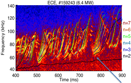
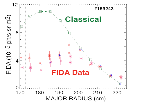
(a)                                                         time of interest(b)

Figure 1: A $CO_{2}$ interferometer power spectra for DIII-D shot $\#159243$ during the current ramp with $6.5MW$ NBI. The spectrum on figure (a) shows multiple sweeping fre quency Reversed Share AEs (RSAE) and steady Toroidicity-induced AE (TAE) modes. Figure (b) compares classical TRANSP predictions for beam ion profile. The graph shows the error bar uncertainty associated with the background subtraction. The two sets of data represent two different light calibrations. The dotted vertical line indicates the location of the magnetic axis. (Figures are reproduced from Ref.Heidbrink et al. (2017))

An interesting feature of the data was revealed later when the velocity space resolution allowed the demonstration of a rather unexpected hollow profile of EP distribution function. The data was collected in part by the Fast Ion D_α (FIDA) diagnostics with some velocity space resolution. A similar feature was found using the interpretive kick model where the integration of the EP distribution function was implemented along the same FIDA “view” window COM path. An application of the critical gradient model Gorelenkov et al. (2016) to the same case did not find any hollow EP profile behaviour but rather monotonic radial EP profiles.

V.1 Perturbative NOVA simulations for RBQ

Since RBQ is essentially perturbative and works as a postprocessor for NOVA/NOVA-K runs, its analysis is initiated by identifying the mode structures of AE instabilities responsible for EP transport. Extensive efforts were already undertaken with the kick model applications recently Heidbrink et al. (2017). We make use of these RSAE/TAE results.

To show the details of RBQ analysis we choose a $n=4$ RSAE from Ref.Heidbrink et al. (2017) for EP distribution relaxation. The mode is localized near $q_{min}\simeq 3$ at $t=805msec$ surface and has one dominant $m=12$ poloidal harmonic which is shown in Fig. 2.

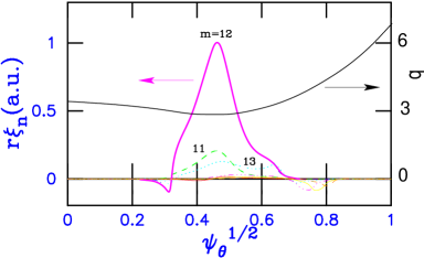
Figure 2: A plot of the $q$-profile of the plasma and spatial structure of poloidal harmonics for the radial displacement $n=4$, $f=84kHz$ RSAE computed by the ideal MHD code NOVA. The mode structure is computed for the plasma equilibrium with the shown safety factor profile.

The ideal MHD NOVA mode structures is used by the NOVA-K code Gorelenkov et al. (1999b) to evaluate the wave particle interaction (WPI) matrices for further processing by the RBQ code as described in Sec.II and the Appendix A. For the RSAE shown in Fig. 2, NOVA-K computes the normalized growth rate $\gamma_{L}/\omega=3.2\%$ and the total damping rate $\gamma_{d}/\omega=-1.81\%$.

As a result the broadening of the resonance line, Eq.(7) is computed at each resonance point within the RBQ code as illustrated in Fig.3. Figure 3 (a) shows 7 resonance lines at one value of $\lambda=0.4$ corresponding to co-passing ions, where $\lambda=\mu B_{0}/\mathcal{E}$ and $B_{0}$ is the magnetic field strength on the axis. Figure 3 (b) shows the broadening of those resonances due to the first and the last terms in Eq.(7).

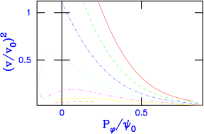
(a)         (b)

Figure 3: Resonance lines of passing EPs interacting with the RSAE mode (the mode structure is shown in Fig.2) in the COM plane: normalized kinetic energy vs. canonical toroidal momentum. Shown in figure (a) are seven dominant resonancies at $\lambda=0.4$. Figure (b) represents the broadening of the resonance lines in the direction of $P_{\varphi}$ computed at the mode amplitude $\delta B/B=7.4\times 10^{-3}$.

The relaxation of EP distribution function (DF) can be computed within the RBQ simulations accurately. However in the present form the RBQ1D code computes the WPI induced diffusion into the TRANSP code through the probability density function (PDF) introduced above (see Sec.IV and also Ref. Podestà et al. (2015)). At the moment we will limit the initial RBQ1D application to such interface with TRANSP.

It has been shown that the kick model captures the EP diffusion in the velocity space which is substantially different from the diffusion “ad-hoc” model used normally in TRANSP and is a significant factor affecting the EP distribution function Podestà et al. (2016a). We employ the AE driven PDFs computed by RBQ within TRANSP and show the obtained results in the next figure 4. The results are for the single RSAE shown in Fig. 2.

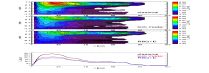
(a)                                        (b) (c) (d)

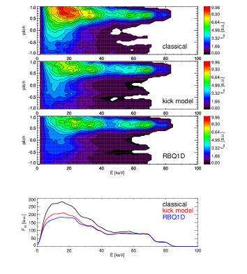
Figure 4: TRANSP simulated EP distribution function in the velocity space for the time of interest, $t=800msec$ using the diffusion computed by RBQ1D and the kick model as indicated. Shown are DF averaged between the normalized poloidal flux $\sqrt{\psi/\psi_{w}}=0.4$ and $0.6$ values, where $\psi_{w}$ is the poloidal magnetic field flux at the wall. Figure (a) shows the pitch angle averaged DF velocity dependance. Figures (b,c,d) correspond to the classical, kick model and RBQ1D simulations of the EP diffusion.

Comparing three cases in the Fig.4 tells us that the effect of AEs is similar on the beam ions if modeled by RBQ1D or by the kick models. Insert (a) tells us that most of the losses are at the low energies, $E_{b}=10-30keV$, where neutrons are generated. This is consistent with the Fig. 3(b) which shows that this is where the resonances are most overlapped which results in stronger radial transport.

RBQ has been implemented in a way which allows either interpretive or predictive analysis. Let us consider them both.

V.2 Interpretive RBQ implementation for TRANSP code

The present mode of RBQ operation relies on AE amplitude values inferred from the experimental measurements. As we mentioned above, the kick model has been successful describing DIII-D FIDA experiments by computing EP diffusion specific to particle position in the COM space Heidbrink et al. (2017). It reproduced the hollow EP pressure profiles as a result. We use the same amplitude values for RBQ1D analysis.

Details of TRANSP computations using PDFs are already published Podestà et al. (2016a, b, 2017), so that here we present the results using those techniques. We add the RBQ prescribed PDFs and summarize this exercise in figure 5. One can see that both models work well by computing beam ion hollow density profils. We should add however that in the inerpretive mode RBQ1D and kick models had additional constraint due to the neutron flux.

Additional studies were done which show the origin of the inverse profile behaviour. We have found that the origin of the reversed profiles is due to the diffusion of copassing beam ions subject to strong diffusion. They are dominating the EP population near the center and are preferentially transported in radial direction outward.

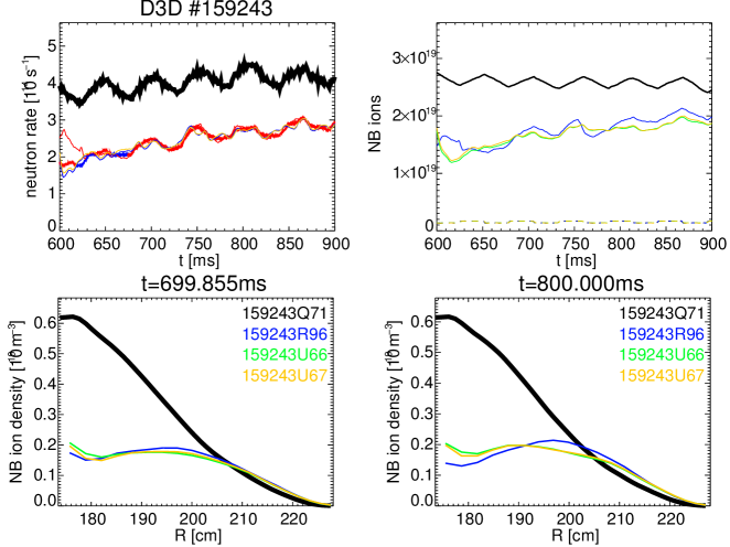
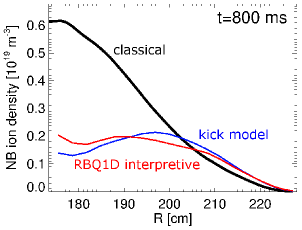
(a)                                                  (b)

Figure 5: Left figure compares the neutron rate computed by TRANSP using various assumptions about EP diffusivities. Top (black, classical) dependence is obtained ignoring EP diffusion. Kick model NBI density profiles are blue curves whereas RBQ1D profile and time dependencies are shown in red.

V.3 Predictive RBQ implementation for TRANSP code

In the predictive RBQ analysis we repeated computations from the previous section V.2 by using the same set of AEs. However we compute AE amplitudes in a different manner by finding their values when the particular mode reaches the saturation, i.e. when the growth rate balances the damping rate, $\gamma_{L,k}=-\gamma_{d,k}$. This way we are not addressing the intermittency in AE transport seen in experiments (see Fig.1), nor do we address the long time scale changes in AE stability as the RSAEs, for example, are sweeping its frequency on a hundred milisecond time scale.

The application of RBQ predictions within the TRANSP simulations are summarized in Figs. 6. After TRANSP turns AE diffusion on at $t=600ms$ the diffusion coefficients are kept constant throughout simulations. Variations in AE amplitudes are reflected by different TRANSP computations. We are showing that the predictive RBQ runs with 0.85 times the amplitude values which fit the best the neutron defiict in TRANSP simulations. The beam density profiles remains hollow within the amplitude variations.

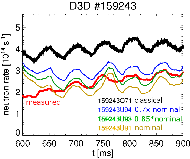
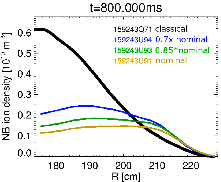
(a)                                                  (b)

Figure 6: The same as in Fig. 5 but computed within the predictive TRANSP analysis. Different EP profile and evolution curves are color coded as indicated on the figure.

VI Summary and future plans

This paper demonstated the effectiveness of the quasi-linear model in its applications for realistic simulations of the beam ion self-induced relaxation via the Alfvénic instabilities. We have summarized the formulation for the Resonance line Broadened QL (RBQ) numerical model with the EP diffusion near the resonances. The formulation can be applied for isolated or for the overlapping modes.

The RBQ1D has been applied in the interpretive and in the predictive mode to DIII-D critical gradient experiments via prescription of the PDF for the beam ions. Initial results show that the model is sound and ready to be applied to predict the fast ion relaxation in burning plasmas. However more validations are required in order to gain the confidence in its predictive capability.

Among the immediate plans we have the development of the RBQ in its 2D version where the EP diffusion paths are sensitive to AE toroidal mode number and its frequency. The number of refined grid points of energetic particle diffusion and the need to resolve the resonances make the 2D problem intrinsically complex and computationally demanding.

Appendix A Linear growth rate as a result of the nonadiabatic component of the distribution function

NOVA Cheng et al. (1985); Gorelenkov et al. (1999b) is a nonvariational, ideal MHD code primarily used to integrate non-Hermitian eigenmode equations in the presence of EPs, using a general flux coordinate system. NOVA-K Cheng (1992) is a stability code used to study the destabilization of TAEs by EPs free energy stored in the gradients of the distribution. The resonance response of energetic particles enter the system through the perturbed pressure associated with them. NOVA makes no use of inverse aspect ratio approximation and hence is well suited to study spherical tokamaks. The code uses Fourier expansion in $\theta$ and cubic spline finite elements in the radial $\psi$ direction. Following the procedure of Cheng Cheng (1992) we may start with the MHD formalism where the fast particle contribution is treated perturbatively, with all perturbed quantities represented in the form

$$A\left(\bm{r},t\right)=\underset{m}{\sum}A_{m}e^{i\left(S_{m}-\omega t\right)};\quad S_{m}\equiv m\theta-n\varphi$$

We shall start with the momentum conservation equation. This equation can be put in a quadratic form if dot multiplied by $\bm{\xi}^{*}$ and integrated over the whole plasma volume. If eqs. (3.15) of Gorelenkov et al. (1999b) are used we get

$$D(\omega)=\delta W_{f}+\delta W_{k}-\delta K=0$$

where the inertial (kinetic) energy is given by $\delta K=\omega^{2}\int\rho\left|\bm{\xi}\right|^{2}d{\bf r}$. $\delta W_{f}$ is the total fluid potential energy and $\delta W_{k}$ is the EPs potential energy . $\omega_{r}\delta W_{k}$ is the power being released by the resonant particles. The quadratic form is particularly useful when stability analysis is addressed. For example, if the mode frequency is assumed to be $\omega=\omega_{r}+i\gamma$, with $\left|\gamma\right|\ll\left|\omega_{r}\right|$, it is obtained Cheng (1992)

$$\gamma\approx\frac{\Im\delta W_{k}}{2\delta K}\omega_{r}$$

In the last equation, it was used that the inertial energy is close to the mode energy. This is because Alfvén waves involve negligible electric field perturbations. Their energy is nearly equally divided between the perturbed magnetic energy and the kinetic energy of particles oscillating as a result of the perturbation.$\Re$ and $\Im$ denote the real and imaginary parts, respectively. $\delta K=\omega^{2}\int\rho\left|\bm{\xi}\right|^{2}d{\bf r}$ accounts for all poloidal harmonics and is simply a number, being a global factor for each toroidal mode number $n$. Since $\rho$ is the total plasma density, it is very little affected by the fast ions density. This number is also provided by NOVA-K. For TAEs, the growth rate is not simple as in the case of an idealized bump-on-tail configuration, being an integral over the resonant curve in phase space and depending on the mode structure. In order to compute $\Im\delta W_{k}$, and consequently $\gamma_{n}$, the non-adiabatic part of the distribution function, $g$, must be calculated. This function can be redefined as $\hat{g}$ to satisfy

$$\frac{d\hat{g}}{dt}=\frac{z}{M}\frac{\partial f}{\partial\mathcal{E}}\left(\omega-\omega_{*}\right)\hat{X}$$

where $\omega_{*}=n\left(\partial f/\partial P_{\varphi}\right)/\left(\partial f/\partial\mathcal{E}\right)$ is the diamagnetic frequency, being a measure of the relation of the radial gradient in the energetic in EP profiles to the velocity gradient. Since $dP_{\varphi}=-\frac{qr}{\omega_{c}}dr$ and the EP density decreases with radius, we have $\frac{\partial f}{\partial P_{\varphi}}>0$. On the other hand, the average energy of EPs also decreases with radius, which implies $\frac{\partial f}{\partial\mathcal{E}}<0$. Therefore, in a tokamak, the free energy stored in the radial gradient drives the mode while the negative gradient in energy tends to stabilize the mode. The mode is unstable when $\omega_{*}>\omega$. $\hat{X}$ is given by

$$\hat{X}=\left(\frac{d{\bf r}_{c}}{dt}-v_{\parallel}\hat{b}\right)J_{0}\nabla\phi_{c}+\frac{i\mu\omega M}{z}\frac{df}{d\mu}\left(J_{0}+J_{2}\right)B_{\parallel c}$$

where the subscript $c$ means that the quantity is evaluated at the particle gyrocenter. The Bessel functions are understood to have the argument $v_{\perp}\nabla_{\perp}/\omega_{c}$, which operates on the perturbed quantities. $v_{\perp}\nabla_{\perp}/\omega_{c}\sim v_{\perp}k_{\perp}/\omega_{c}\ll 1$ which justifies the Taylor expansion of the Bessel functions, $J_{\alpha}\left(v_{\perp}\nabla_{\perp}/\omega_{c}\right)\rightarrow\overset{\infty}{\underset{j=0}{\sum}}\frac{\left(-1\right)^{j}}{j!\Gamma\left(j+\alpha+1\right)}\left(v_{\perp}\nabla_{\perp}/\omega_{c}\right)^{2j+\alpha}$. If ${\bf E}_{\perp}=-\nabla\phi$ (${\bf A}_{\perp}$ contribution neglected) we can write

$$\hat{X}\simeq\frac{i\omega M}{z}\left[\left(2\mathcal{E}-3\mu B\right)J_{0}\bm{\kappa}\cdot\bm{\xi}_{\perp}-\mu BJ_{0}\nabla\cdot\bm{\xi}_{\perp}\right]$$

where $\bm{\kappa}$ stands for the curvature. The solution of the drift kinetic equation can be written as

$$\hat{g}=\frac{z}{M}\intop^{t}\frac{\partial f}{\partial\mathcal{E}}\left(\omega-\omega_{*}\right)\hat{X}dt^{\prime}$$

where the time integration is along the particle trajectory. Assuming $S_{m}(t=0)=0$, one can write in terms of the following Fourier series

$$\hat{X}=\sum_{m,l}e^{-i\omega t+i\overline{\omega}_{Dm}t}X_{ml}e^{il\omega_{\theta}t}$$

$$X_{ml}=\frac{1}{\tau_{b}}\oint dt^{\prime}\hat{X}e^{i\intop^{t^{\prime}}\left(\omega_{Dm}-\overline{\omega}_{Dm}-l\omega_{\theta}\right)dt^{\prime\prime}}$$

$\Im\delta W_{k}$ can then be calculated from

$$\delta W_{k}=-\int\int\hat{g}{\bf v}\cdot\left({\bf v}\cdot\nabla\right)\xi^{*}d{\bf r}_{c}d{\bf v}=-\frac{iz}{\omega}\int\int\hat{X}^{*}\hat{g}d{\bf r}_{c}d{\bf v}$$

The phase-space integration is given by

$$\begin{array}[]{c}\intop d\Gamma...=\int d^{3}J\int d^{3}\Theta...=\left(2\pi\right)^{3}\int d^{3}J\underset{l}{\sum}...=\\ =\int d{\bf r}_{c}\int d{\bf v}...=\left(2\pi\right)^{2}\underset{\sigma_{\parallel}}{\sum}\frac{B}{\omega_{c}}\int dP_{\varphi}\int d\mathcal{E}\int d\mu\int dt...,\end{array}$$

with $dt$ being associated to the fast particle orbital motion. The integrals over $\varphi$ and $\theta_{g}$ will contribute with $2\pi$ each. Note that in NOVA, $P_{\varphi}$, $\mathcal{E}$ and $\mu$ are defined without the mass. If they had usual units, we would have $\int d{\bf r}_{c}\int d{\bf v}...=\left(2\pi\right)^{2}\left(\frac{c}{zM^{2}}\right)\underset{\sigma_{\parallel}}{\sum}\int dP_{\varphi}\int d\mathcal{E}\int d\mu\int dt...$ . We can write

$$\hat{g}=\frac{iz}{M}\sum_{m,l}\frac{e^{-i\omega t+i\overline{\omega}_{Dm}t+il\omega_{\theta}t}}{\omega-\overline{\omega}_{Dm}-l\omega_{\theta}}\frac{\partial f}{\partial\mathcal{E}}\left(\omega-\omega_{*}\right)X_{ml}$$

Therefore

$$\delta W_{k}=-\frac{\left(2\pi M\right)^{2}c\omega}{z}\underset{\sigma_{\parallel}}{\sum}\int dP_{\varphi}d\mu d\mathcal{E}dt\sum_{m,m^{\prime},l,l^{\prime}}G_{m^{\prime}l}^{*}\frac{\mathcal{E}^{2}\left(\frac{\partial f}{\partial\mathcal{E}}\right)\left(1-\nicefrac{{\omega_{*}}}{{\omega}}\right)}{\omega-\overline{\omega}_{Dm}-l\omega_{\theta}}G_{ml}e^{-it\left(\overline{\omega}_{Dm^{\prime}}-\overline{\omega}_{Dm}+\left(l^{\prime}-l\right)\omega_{\theta}\right)}$$

where the “drift” frequency is $\omega_{Dm}\equiv\frac{dS_{m}}{dt}$ and $\overline{\omega}_{Dm}$ means orbit averaged drift frequency, The matrix elements are defined as $G_{ml}=-i\frac{zX_{ml}}{\omega M\mathcal{E}}$. The Plemelj formula could be used to develop the denominator. So, the imaginary part of $\delta W_{k}$ becomes

$$\Im\delta W_{k}=\frac{\left(2M\right)^{2}\pi^{3}c\omega_{r}}{z}\int dP_{\varphi}d\mu d\mathcal{E}\sum_{m,m^{\prime},l}G_{m^{\prime}l}^{*}\mathcal{E}^{2}\tau_{b}\left(\frac{\partial f}{\partial\mathcal{E}}\right)\left(1-\nicefrac{{\omega_{*}}}{{\omega_{r}}}\right)G_{ml}\delta\left(\omega_{r}-\overline{\omega}_{D0}-l\omega_{\theta}\right)$$

The growth rate in NOVA is then given by:

$$\gamma=\frac{\left(2M\right)^{2}\pi^{3}c\omega^{2}}{2z\omega^{2}\int\rho\left|\bm{\xi}\right|^{2}d{\bf r}}\underset{\sigma_{\parallel}}{\sum}\int dP_{\varphi}d\mu d\mathcal{E}\sum_{m,m^{\prime},l}G_{m^{\prime}l}^{*}\mathcal{E}^{2}\tau_{b}\left(\frac{\partial f}{\partial\mathcal{E}}-\frac{n}{\omega}\frac{\partial f}{\partial P_{\varphi}}\right)G_{ml}\delta\left(\omega-\overline{\omega}_{D0}-l\omega_{\theta}\right)$$

Now we want to compare the growth rate in NOVA and in Kaufman’s normal mode theory, in order to be able to relate their respective mode structure information ($G$ and $\alpha_{{\bf l}}$) and build a quasilinear theory based on that. Using $\delta K=\omega^{2}\int\rho\left|\bm{\xi}\right|^{2}d{\bf r}$, the comparison leads to $\frac{M\mathcal{E}\omega}{\sqrt{2}}\sum_{m}G_{ml}\equiv\int d^{3}x\mathbf{e}\left(\mathbf{x},\omega\right)\cdot{\bf j_{l}}\left({\bf x}\mid{\bf J}\right)=\frac{\omega}{i}V_{{\bf l}}$ or, alternatively

$$\alpha_{{\bf l}}\left({\bf J}\right)=\left(\frac{M\mathcal{E}\omega}{\sqrt{2}}\right)^{2}\sum_{m,m^{\prime}}G_{m^{\prime}l}^{*}G_{ml}=\omega^{2}\left|V_{{\bf l}}\right|^{2}$$ (20)

where

$$V_{l}=\frac{iz}{\omega}\int\frac{d^{3}\Theta}{(2\pi)^{3}}\mathbf{e}\left(\mathbf{r},\omega\right)\cdot{\bf v}\left({\bf J},\bm{\Theta}\right)e^{-i\mathbf{l}\cdot\bm{\Theta}}$$

which is consistent with the expression given in Berk et al. (1997). The mode structure is provided in NOVA via the $G$ matrices. They are calculated via time integration that account for the eigenmode felt by a particle in a given trajectory. A weighted integration is performing according to how much time a particle spends at each position of its trajectory. Mirror-trapped particles have their parallel velocity reversed at the tips of a banana orbit, where they tend to remain longer and consequently the local mode structure will have an important contribution for the overall integration. By using equation (20) we can now express the quasilinear diffusion equation, (2) and (3), in terms of NOVA code notation.

Appendix B Expected saturation levels from a single mode perturbation theory

For a single, isolated mode in a simplified bump-on-tail situation, at the saturation ($\gamma_{L}\simeq\gamma_{d}$, $\partial f/\partial t=0$), we have

$$\frac{\pi}{2}\omega_{b}^{4}\mathcal{F}\frac{\partial f}{\partial\Omega}+\nu_{scatt}^{3}\frac{\partial(f-f_{0})}{\partial\Omega}=0.$$

Analytic results far from and close to marginal stability can be used to lead the choice of the broadening parameters Ghantous et al. (2014a); Ghantous (2013). For the case of a flat-topped window function, $\mathcal{F}=1/\Delta\Omega$, we have

$$\Delta\Omega=\frac{\pi}{2}\frac{\omega_{b}^{4}}{\nu_{scatt}^{3}}\frac{\gamma_{d}}{\gamma_{L,0}-\gamma_{d}}.$$ (21)

Near marginal stability

For this case $\Delta\Omega\approx c\nu_{scatt}$. The expected saturation level from analytical theory for the case $\omega_{b}/\nu_{scatt}\ll 1$ to be Berk et al. (1996b); Gorelenkov et al. (1999a)

$$\omega_{b}\simeq 1.18\nu_{scatt}\left(\frac{\gamma_{L}}{\gamma_{d}}-1\right)^{1/4},$$

which, when substituted in (21) leads to $a=2.7$.

Far from marginal stability

For this case $\Delta\Omega\approx a\omega_{b}$. The expected saturation level from analytical theory for the case $\omega_{b}/\nu_{scatt}\gg 1$ is Berk and Breizman (1990b); Gorelenkov et al. (1999a)

$$\omega_{b}\simeq 1.2\nu_{scatt}\left(\frac{\gamma_{L}}{\gamma_{d}}\right)^{1/3},$$

which, when substituted in (21) leads to $c=2.5$. There are no known analytical solutions to rely on in order to determine the constant $b$. It was simply taken equal to $c$ in previous works Ghantous et al. (2014a); Ghantous (2013); Berk et al. (1996a, 1995). We have verified that the saturation levels obtained numerically with RBQ are not sensitive with respect to the exact value of $b$. This is because as the mode starts its growth, the term $c\nu_{scatt}$ has been observed to be the dominant broadening component for practical cases, as inferred by NOVA-K. On he other hand, as the mode approaches saturation, the term $a\omega_{b,n}$ outweights $b\left|\gamma_{L,n}-\gamma_{d,n}\right|$ since the latter approaches zero. The study of the parametric dependencies of the broadened window for realistic eigenmodes is under way Meng et al. (2018) using the guiding-center, particle following code ORBIT White and Chance (1984).

References

- Gorelenkov et al. (2014) N. N. Gorelenkov, S. D. Pinches, and K. Toi, Nucl. Fusion 54, 125001 (2014).
- Duarte (2017) V. N. Duarte, Quasilinear and nonlinear dynamics of energetic-ion-driven Alfvén eigenmodes, http://www.teses.usp.br/teses/disponiveis/43/43134/tde-01082017-195849/, Ph.D. thesis, University of São Paulo, São Paulo, Brazil (2017).
- Collins et al. (2016) C. S. Collins, W. W. Heidbrink, M. E. Austin, G. J. Kramer, D. C. Pace, C. C. Petty, L. Stagner, M. A. Van Zeeland, R. B. White, Y. B. Zhu, and The DIII-D team, Phys. Rev. Letters 116, 095001 (2016).
- Heidbrink et al. (2008) W. W. Heidbrink, M. A. Van Zeeland, M. E. Austin, K. H. Burrell, N. N. Gorelenkov, G. J. Kramer, Y. Luo, M. A. Makowski, G. R. McKee, C. Muscatello, R. Nazikian, E. Ruskov, W. M. Solomon, R. B. White, and Y. Zhu, Nucl. Fusion 48, 084001 (2008).
- Drummond and Pines (1962) W. Drummond and D. Pines, Nucl. Fusion Suppl. 2, Pt. 3 (1962).
- Vedenov et al. (1961) A. A. Vedenov, E. P. Velikhov, and R. Z. Sagdeev, Sov. Phys. Uspekhi 4, 332 (1961).
- Duarte et al. (2017a) V. N. Duarte, H. L. Berk, N. N. Gorelenkov, W. W. Heidbrink, G. J. Kramer, R. Nazikian, D. C. Pace, M. Podestà, B. J. Tobias, and M. A. Van Zeeland, Nuclear Fusion 57, 054001 (2017a).
- Duarte et al. (2017b) V. N. Duarte, H. L. Berk, N. N. Gorelenkov, W. W. Heidbrink, G. J. Kramer, R. Nazikian, D. C. Pace, M. Podestà, and M. A. V. Zeeland, Physics of Plasmas 24, 122508 (2017b), https://doi.org/10.1063/1.5007811 .
- Kaufman (1972) A. N. Kaufman, Phys. Fluids 15, 1063 (1972).
- Chirikov (1960) B. Chirikov, Journal of Nuclear Energy. Part C, Plasma Physics, Accelerators, Thermonuclear Research 1, 253 (1960).
- Berk et al. (1995) H. L. Berk, B. N. Breizman, J. Fitzpatrick, and H. V. Wong, Nucl. Fusion 35, 1661 (1995).
- Berk et al. (1996a) H. L. Berk, B. N. Breizman, J. Fitzpatrick, M. S. Pekker, H. V. Wong, and K. L. Wong, Phys. Plasmas 3, 1827 (1996a).
- Meng et al. (2018) G. Meng, N. N. Gorelenkov, V. N. Duarte, H. L. Berk, R. B. White, and X. Wang, Nuclear Fusion (2018), 10.1088/1741-4326/aaa918.
- Fitzpatrick (1997) J. Fitzpatrick, A Numerical Model of Wave-Induced Fast Particle Transport in a Fusion Plasma, Ph.D. thesis, University of California, Berkeley, Berkeley, CA (1997).
- Ghantous et al. (2014a) K. Ghantous, H. L. Berk, and N. N. Gorelenkov, Phys. Plasmas 21, 032119 (2014a), http://dx.doi.org/10.1063/1.4869242.
- Ghantous (2013) K. Ghantous, Reduced Quasilinear Models for Energetic Particles Interaction with Alfvén Eigenmodes, Ph.D. thesis, Princeton University (2013).
- Heidbrink et al. (2017) W. W. Heidbrink, C. S. Collins, M. Podestà, G. J. Kramer, D. C. Pace, C. C. Petty, L. Stagner, M. A. Van Zeeland, R. B. White, and Y. B. Zhu, Phys. Plasmas 24, 056109 (2017).
- Podestà et al. (2014) M. Podestà, M. V. Gorelenkova, and R. B. White, Plasma Phys. Control. Fusion 56, 055003 (2014).
- Podestà et al. (2017) M. Podestà, M. Gorelenkova, N. N. Gorelenkov, and R. B. White, Plasma Phys. Control. Fusion 59, 095008 (2017).
- Goldston et al. (1981) R. J. Goldston, D. C. McCune, H. H. Towner, S. L. Davis, R. J. Hawryluk, and G. L. Schmidt, J. Comput. Phys. 43, 61 (1981).
- Dupree (1966) T. H. Dupree, Physics of Fluids 9, 1773 (1966).
- White et al. (2010) R. B. White, N. N. Gorelenkov, W. W. Heidbrink, and M. A. Van Zeeland, Plasma Phys. Control. Fusion 53, 045012 (2010).
- Berk and Breizman (1990a) H. L. Berk and B. N. Breizman, Physics of Fluids B: Plasma Physics 2, 2235 (1990a), http://dx.doi.org/10.1063/1.859405 .
- Berk et al. (1997) H. L. Berk, B. N. Breizman, and M. S. Pekker, Plasma Phys. Reports 23, 778 (1997).
- Gorelenkov et al. (1999a) N. N. Gorelenkov, Y. Chen, R. B. White, and H. L. Berk, Phys. Plasmas 6, 629 (1999a).
- Ghantous et al. (2014b) K. Ghantous, H. L. Berk, and N. N. Gorelenkov, Phys. Plasmas 21, 032119 (2014b).
- Pankin et al. (2004) A. Pankin, D. McCune, R. Andre, and et.al., Comp. Phys. Communications 159, 157 (2004).
- Podestà et al. (2016a) M. Podestà, M. Gorelenkova, E. D. Fredrickson, N. N. Gorelenkov, and R. B. White, Nuclear Fusion 56, 112005 (2016a).
- Podestà et al. (2016b) M. Podestà, M. Gorelenkova, E. D. Fredrickson, N. N. Gorelenkov, and R. B. White, Phys. Plasmas 23, 056106 (2016b).
- White and Chance (1984) R. B. White and M. S. Chance, Phys. Fluids 27, 2455 (1984).
- White (2011) R. B. White, Plasma Phys. Control. Fusion 53, 085018 (2011).
- White (2012) R. B. White, Commun. Nonlinear Sci. Numer. Simulat. 17, 2200 (2012).
- Gorelenkov et al. (2016) N. N. Gorelenkov, W. W. Heidbrink, G. J. Kramer, J. B. Lestz, M. Podestà, M. A. Van Zeeland, and R. B. White, Nucl. Fusion 56, 112015 (2016).
- Gorelenkov et al. (1999b) N. N. Gorelenkov, C. Z. Cheng, and G. Y. Fu, Phys. Plasmas 6, 2802 (1999b).
- Podestà et al. (2015) M. Podestà, M. V. Gorelenkova, D. S. Darrow, E. D. Fredrickson, S. P. Gerhardt, and R. B. White, Nucl. Fusion 55, 053018 (2015).
- Cheng et al. (1985) C. Z. Cheng, L. Chen, and M. S. Chance, Ann. Phys. 161, 21 (1985).
- Cheng (1992) C. Z. Cheng, Phys. Reports 211, 1 (1992).
- Note (1) In NOVA-K, both potential and kinetic energies are defined as twice their actual values. This can be seen from comparing equations (3.69) and (3.70) of Cheng (1992) with equations (4.19) and (4.31) of White (2013). This choice does not introduce changes to the growth rate.
- Berk et al. (1996b) H. L. Berk, B. N. Breizman, and M. S. Pekker, Phys. Rev. Letters 76, 1256 (1996b).
- Berk and Breizman (1990b) H. L. Berk and B. N. Breizman, Physics of Fluids B: Plasma Physics 2, 2246 (1990b), http://dx.doi.org/10.1063/1.859406 .
- White (2013) R. B. White, The Theory of Toroidally Confined Plasmas, 3rd ed. (Imperial College Press, London, UK, 2013).