Kernel-nulling for a robust direct interferometric
detection of extrasolar planets

Abstract

Context. Combining the resolving power of long-baseline interferometry with the high-dynamic range capability of nulling still remains the only technique that can directly sense the presence of structures in the innermost regions of extrasolar planetary systems.

Aims. Ultimately, the performance of any nuller architecture is constrained by the partial resolution of the on-axis star whose light it attempts to cancel out. However from the ground, the effective performance of nulling is dominated by residual time-varying instrumental phase and background errors that keep the instrument off the null. Our work investigates robustness against instrumental phase.

Methods. We introduce a modified nuller architecture that enables the extraction of information that is robust against piston excursions. Our method generalizes the concept of kernel, now applied to the outputs of the modified nuller so as to make them robust to second order pupil phase error. We present the general method to determine these kernel-outputs and highlight the benefits of this novel approach.

Results. We present the properties of VIKiNG: the VLTI Infrared Kernel NullinG, an instrument concept within the Hi-5 framework for the 4-UT VLTI infrastructure that takes advantage of the proposed architecture, to produce three self-calibrating nulled outputs.

Conclusions. Stabilized by a fringe-tracker that would bring piston-excursions down to 50 nm, this instrument would be able to directly detect more than a dozen extrasolar planets so-far detected by radial velocity only, as well as many hot transiting planets and a significant number of very young exoplanets.

1 Introduction

The direct imaging of extrasolar planets from the ground remains an incredibly challenging objective that requires the simultaneous combination of high angular resolving power, required to see objects separated by a few astronomical units and located tens of parsecs away, with high-dynamic imaging capability to overcome the large contrast between the faint planet and its bright host star. This objective is doubly limited by the phenomenon of diffraction, that sets a limit to the resolving power of a telescope or interferometer, and produces diffraction features such as rings, spikes, fringes and speckles whose contribution to the data dominates that of the faint structures one attempts to detect, by several orders of magnitude.

A high-contrast imaging device, be it a coronagraph (Lyot, 1932) when observing with a single telescope or a nuller (Bracewell, 1978) when using an interferometer, is a contraption devised to attenuate the static diffraction-induced signature of one bright object in the field, while transmitting the rest of the field. Very elegant and effective solutions have been devised (Guyon, 2003; Soummer, 2005; Mawet et al., 2010), that can theoretically deliver data where the contribution of the bright star is attenuated to up to ten orders of magnitudes (Trauger & Traub, 2007) and a few such coronagraphs are currently in operation on ground based observing facilities. Their high-contrast imaging capability is however severely affected by the less than ideal conditions they experience when observing through the atmosphere, even (Aime & Soummer, 2004) with correction provided by state-of-the-art extreme adaptive optics (XAO) systems like VLT/SPHERE (Beuzit et al., 2006), the Gemini Planet Imager (Macintosh et al., 2014) or the Subaru Telescope SCExAO (Jovanovic et al., 2015).

The position of an aberration-induced speckle in the field is related to a sinusoidal wavefront modulation across the aperture of the instrument, and the contrast $c$ of this speckle at wavelength $\lambda$ is directly related to the amplitude $a$ of the modulation, using the following simple relation:

$$c=\left(\frac{2\pi a}{\lambda}\right)^{2},$$ (1)

which can be used to estimate how to translate a raw-contrast objective into a requirement on the wavefront stability. Thus, regardless of the architecture of the high-contast device, a raw contrast $c=10^{-6}$ ambition for an instrument observing in the H-band ($\lambda=1.6\,\mu$m) translates into a wavefront quality requirement better than 0.25 nm, which is more than two orders of magnitude beyond what state of the art XAO systems are able to deliver (Sauvage et al., 2016).

Reported recent detections of extrasolar planet companions (Macintosh et al., 2015; Chauvin et al., 2017), owe much to post-processing techniques such as angular differential imaging (Marois et al., 2006) that make it possible to disantangle genuine structures present in the image from residual diffraction features (Marois et al., 2008) that otherwise dominate it. To increase the impact of the high-contrast device in the pre-processing stage, one approach might be to look into solutions that do not necessarily produce the highest performance when operating in ideal but rarely occuring observing conditions, but instead integrate some form of robustness against small perturbations. The work described in this paper is a step in this direction.

An alternative observing technique to XAO-fed coronagraphy for high-contrast detection of extrasolar planets is to use long-baseline nulling-interferometry. Thanks to their higher angular resolution, long-baseline nulling interferometers allow the observation of planets much closer to the star than coronagraphs or to use a longer mid-infrared wavelength, where the expected star-planet contrast is expected to be more favorable (Charbonneau et al., 2005). Very much like for ground-based coronagraphy, the effective actual high-contrast detection potential of nulling is constrained by variable observing conditions, that result in fluctuations of the thermal background as well as small piston excursions, minimized by fringe tracking, that keep the observation off the null (Serabyn et al., 2012). For instance, N-band nulling instruments such as the Keck Interferometric Nuller (KIN) and the Large Binocular Telescope Interferometer (LBTI) are limited to constrasts of a few $10^{-4}$ to a few $10^{-3}$ by residual background errors (e.g., Colavita et al. (2009); Defrère et al. (2016), while at shorter wavelength the Palomar Fiber Nuller (PFN) was limited to contrast of a few $10^{-4}$ due to high-frequency residual phase errors (Mennesson et al. 2011). Here too, post-acquisition analysis of the distribution of the measured null (Hanot et al., 2011; Mennesson et al., 2011) make it possible to further characterize the true null depth and improve the contrast detection limits, an approach refered to as Null Self-Calibration (NSC). This approach requires a nuller to detect off-null light with high signal-to-noise within an instrumental coherence time, so is not applicable to observations anywhere near the shot-noise limit of a nulling instrument. It is also currently not applicable to array configurations with more than two telescopes.

Instead, and similarly to high-contrast imaging, pre-processing techniques can be used to improve the null depth and its robustness against perturbations. Over the years, the original idea of Bracewell (1978) has been refined to improve the rejection of the nuller, usually by simultaneously combining more than two apertures (Angel & Woolf, 1997) and optimizing the internal structure of the nuller (Guyon et al., 2013). However, a major limiting factor in exploring these multi-aperture designs has been the difficulty in creating optical devices of sufficient precision and complexity. One avenue which has shown rapid recent process is mid-infrared photonic beam combination, both in ultrafast laser inscription lithography in chalcogenide (Tepper et al., 2017) and fluoride (Gross et al., 2015) substrates, and in planar photolithography based devises using chalcogenide glass (Kenchington Goldsmith et al., 2017) and lithium niobate (Hsiao et al., 2009; Martin et al., 2014). These emerging technological platforms are in need of clear required performance metrics and baseline architectures to define succesful technological development for astrophysics.

In this paper, we present a true self-calibration technique, more akin to the properties of observable quantities like closure-phase (Jennison, 1958), which takes advantage of the coupling between atmospheric induced piston errors along baselines forming a triangle, to produce from a finite set of polluted raw phase measurements, a subset of clean observable quantities, robust against residual piston errors. Shown to be usable in the optical regime (Baldwin et al., 1986), it is extensively used during non-redundant aperture masking interferometry observations (Tuthill et al., 2000) and also takes advantage of the correction provided by AO (Tuthill et al., 2006), as it enables long exposure observations with improved sensitivity. Using closure-phase, VLTI/PIONIER observations achieve contrast detection limits of a few $10^{-3}$ (Absil et al., 2011) alone, without a nuller. The notion of closure-phase was later shown to be a special case of kernel-phase (Martinache, 2010): instead of looking for closure triangles in an aperture, one treats the properties of an interferometer globally, using a single linear operator $\mathbf{A}$ to describe the way instrumental phase propagates in the relevant observable parameter space (the Fourier-phase, in the case of kernel-phase), and looks for linear combinations of polluted data that reside in a space orthogonal to the source of perturbation, described by the row-space of $\mathbf{A}$.

This paper describes how the design of a nuller can be modified to take the possibility of self-calibration into account, to produce observable quantities that are robust against second-order atmospheric-piston-induced phase excursions. The paper uses a generic recipe that is applied to a four-beam nulling combiner, which is the most relevant case for exploiting the capabilities of the existing Very Large Telescope Interferometer (VLTI), within the framework recently provided by the Hi-5 project (Defrère et al., 2018a).

2 Enabling self-calibration for a nuller

2.1 Nuller design and parametrisation

The nuller we are looking at is a combiner taking four inputs of identical collecting power and designed to produce one bright output and three dark ones. This design ignores the true location of the sub-apertures making up the interferometric array, and how these can impact the order of the null (Guyon et al., 2013).

Such a four-beam nuller can be represented by a 4x4 matrix $\mathbf{N}$, acting on the four input complex amplitudes collected by the four apertures, and producing the expected outputs. For the nuller we consider here:

$$\mathbf{N}=\frac{1}{\sqrt{4}}\times\begin{bmatrix}1&1&1&1\\ 1&1&-1&-1\\ 1&-1&1&-1\\ 1&-1&-1&1\end{bmatrix}.$$ (2)

Except for the first row of this matrix for which the input complex amplitudes are constructively combined, each row combines differences of complex amplitudes that would result, for a single on-axis unresolved source and in the absence of atmospheric piston, in a dark output. The global $1/\sqrt{4}$ (=0.5) coefficient makes $\mathbf{N}$ a complex unitary matrix, accounting for the fact that the interferometric recombination process preserves total flux: $||\mathbf{N}\cdot x||^{2}=||x||^{2}$. We have also considered a 4x4 matrix that is constructed from two 2x2 nullers, where the bright outputs are hierarchically combined in a second 2x2 nuller. The result from that architecture is less symmetrical, but is not qualitatively different from the results presented here.

Whereas the raw interferometric phase per baseline is linearly related to the instrumental phase, making the definition of closure- and kernel-phase reasonably direct, the output of a nuller is a quadratic function of piston excursions (Serabyn et al., 2012). Of the four sub-apertures, one, labeled $T_{0}$ is chosen as a phase reference so that phase or piston values are quoted relative to this sub-aperture. The remaining degrees of freedom form a three-parameter (correlated) piston vector $p$ that translates into the chromatic phase $\varphi=2\pi p/\lambda$. Assuming that the source is unresolved by the interferometer, a first order Taylor expansion of piston dependance of the input electric field simply writes as:

$$E_{k}=\exp{(-j\varphi_{k})}\approx 1-j\varphi_{k}.$$ (3)

Plugging these electric field as inputs to the nulling matrix $\mathbf{N}$, one can write the equations for the three nulled intensities, valid to second order in input phase:

$$\mathbf{x}=\frac{1}{4}\times\begin{bmatrix}(\varphi_{1}-\varphi_{2}-\varphi_{3})^{2}\\ (-\varphi_{1}+\varphi_{2}-\varphi_{3})^{2}\\ (-\varphi_{1}-\varphi_{2}+\varphi_{3})^{2}\end{bmatrix}.$$ (4)

Further expansion shows that the piston induced leak of the nuller is a function of six parameters: three second order terms $(\varphi_{k})^{2}$ and three crossed-terms $\varphi_{k}\times\varphi_{l}$. With only the three relations summarized by Equation 4, the problem is underconstrained and does not permit the building of a set of kernels. To build kernels from the output of a combiner, one needs to further break down each nuller output into two non-symmetric outputs that will help discriminate variations in the two parts of the complex visibilities, when properly mixed. This split-and-mix operation can be represented by the following complex linear operator $\mathbf{S}$ that enables the proper sensing of the nuller output:

$$\mathbf{S}=\frac{1}{\sqrt{4}}\times\begin{bmatrix}1&e^{i\theta}&0\\ -e^{-i\theta}&1&0\\ 1&0&e^{i\theta}\\ -e^{-i\theta}&0&1\\ 0&1&e^{i\theta}\\ 0&-e^{-i\theta}&1\end{bmatrix},$$ (5)

where $\theta$ is a pre-defined phase offset and $1/\sqrt{4}$ (= 0.5) a factor that accounts for the total flux preservation when splitting each nulled output into four. A detector placed downstream of this final function records a now six-component intensity vector $\mathbf{x}$ recording the square modulus associated to each output.

A practical implementation of a nuller has to deal with not only residual starlight and phase-noise, but also fluctuating backgrounds and detector noise. This means that a temporal modulation function is also required in addition to the nulling function. Figure 1 shows a schematic representation of a possible interface between the two functions. By modulating the phase shifters, the 6 nulled outputs can be rapidly permuted, enabling the final signal to be obtained from synchronously demodulated outputs. In addition, for faint targets, the starlight may not clearly be detectable above a variable thermal background, meaning that even the star light channel may need to be modulated, in order to apply the correct normalisation to the planet light outputs. In any case, maintaining long-term amplitude balance between the inputs requires either modulation or independent photometric channels.

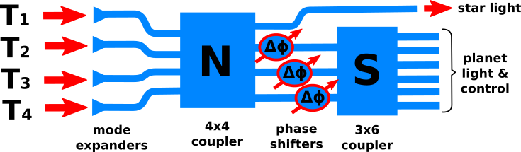
Figure 1: Schematic representation of the proposed two-stage nuller architecture. The first 4x4 coupler stage implements the nulling function described by the matrix $\mathbf{N}$ introduced in Section 2.1. The second 3x6 coupler implements the sensing function described by the matrix $\mathbf{S}$. In between the two stages, modulated phase shifters are inserted so as to eliminate background fluctuations.

The concept described in the rest of the paper will ignore these background fluctuations considerations and the modulation that would otherwise be required to account for it: the nulling and sensing functions can therefore be combined into a single six-by-four operator $\mathbf{M}$ that takes the four input complex amplitudes incoming from the four telescopes and produces six nulled output complex amplitudes:

$$\mathbf{M}=\frac{1}{4}\times\begin{bmatrix}1+e^{i\theta}&1-e^{i\theta}&-1+e^{i\theta}&-1-e^{i\theta}\\ 1-e^{-i\theta}&-1-e^{-i\theta}&1+e^{-i\theta}&-1+e^{-i\theta}\\ 1+e^{i\theta}&1-e^{i\theta}&-1-e^{i\theta}&-1+e^{i\theta}\\ 1-e^{-i\theta}&-1-e^{-i\theta}&-1+e^{-i\theta}&1+e^{-i\theta}\\ 1+e^{i\theta}&-1-e^{i\theta}&1-e^{i\theta}&-1+e^{i\theta}\\ 1-e^{-i\theta}&-1+e^{-i\theta}&-1-e^{-i\theta}&1+e^{-i\theta}\end{bmatrix}.$$ (6)

A detector placed downstream of the combiner now records a six-component intensity vector $\mathbf{x}=||\mathbf{M}\cdot\mathbf{E}||^{2}$. To compare the properties of this modified nuller design to those of the classical one, Figure 2 presents a series of transmission curves of the two nullers for an in-line non-redundant array of coordinates listed in Table 1, and observing in the L-band ($\lambda=3.6\,\mu$m), as a function of source position offset relative to the null. The phase shifting parameter of the mixing function will from now on be set to $\theta=\pi/2$, as this specific value allows to write all matrices explicitly.

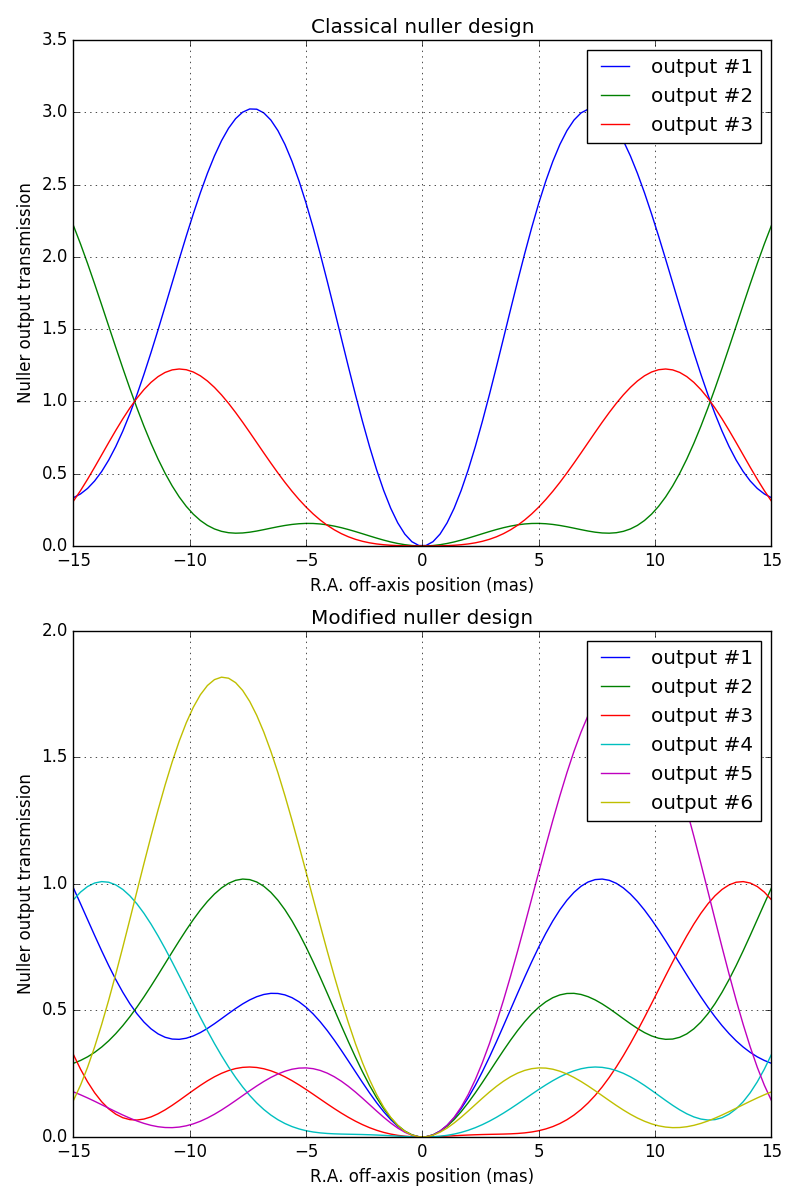
Figure 2: Comparison of the outputs of two nuller architectures as a function of right-ascension (R.A.) offset in milli-arcsecond (mas) for an in-line non-redundant array (aperture coordinates listed in Table 1): the classical design, corresponding to the three nulled outputs of the matrix $\mathbf{N}$ is at the top and the modified design, incorporating the mixing function described in the main text of the paper is at the bottom. In both cases, the output unit is in multiples of the transmission of a single telescope.

Table 1: East and North coordinates (in meters) for a fictive non-redundant linear array, used in Sections 2.1 and 2.2 to illustrate some properties of the proposed nuller architecture.

Station	E	N
T1	0.0	0.00
T2	10.0	0.00
T3	40.0	0.00
T4	60.0	0.00

On-axis, the proposed architecture still behaves like a nuller with zero transmission when operating in perfect conditions. Besides the expected multiplication of outputs going from the classical to the modified nuller design, a major difference lies in the symmetry properties of the outputs: whereas the classical nuller features response curves that are symmetric relative to the on-axis reference, the modified nuller outputs are anti-symmetric and therefore allow to discriminate a positive from a negative offset position, and give a stronger constraint on the position of a companion around a bright star, from a single observation.

2.2 Kernel-nulling

The motivation for the proposed architecture is the ability to build from the six outputs of the combined for each acquisition, a sub-set of observable quantities that exhibit some further robustness against residual piston errors. In a classical (ie. non-nulling) combiner, the four input beam interferometer gives access to up to six distinct baselines that can produce up to three-closure phases (Monnier, 2000), so one expects a satisfactoy nuller architecture should produce three kernels on a non-redundant array.

With one of the four sub-apertures chosen as zero-reference for the phase, the aperture phase of a coherent point-like source reduces to a three-component vector $\varphi$. When everything is in phase ($\varphi=0$), the system sits on the null, where the first order derivative terms of both phase and amplitude are all zeros (see the bottom panel of Fig. 2). Piston-induced leaked intensity $\Delta\mathbf{x}$ by the nuller will therefore be dominated by second order terms, whose impact can be estimated by measuring the local curvature. With three degrees of freedom, six second order terms need to be accounted for: three second-order partial derivatives and three second-order mixed derivatives.

The response of the six intensity outputs to these six second-order perturbations is recorded in a $6\times 6$ matrix $\mathbf{A}$, analoguous to the phase transfer matrix introduced by Martinache (2010) to find the kernel of the information contained in the Fourier-phase, but generalized to encode the impact of second-order differences in the pupil plane phase vector on the output of a nuller:

$$\Delta\mathbf{x}=\mathbf{A}\cdot\left[\frac{\partial^{2}\mathbf{x}}{\partial\varphi_{1}^{2}},\frac{\partial^{2}\mathbf{x}}{\partial\varphi_{2}^{2}},\frac{\partial^{2}\mathbf{x}}{\partial\varphi_{3}^{2}},\frac{\partial^{2}\mathbf{x}}{\partial\varphi_{1}\partial\varphi_{2}},\frac{\partial^{2}\mathbf{x}}{\partial\varphi_{1}\partial\varphi_{3}},\frac{\partial^{2}\mathbf{x}}{\partial\varphi_{2}\partial\varphi_{3}}\right]^{T}.$$ (7)

Just like in the case of kernel-phase, depending on the properties of $\mathbf{A}$, it may be possible to identify a sub-set of linear combinations of rows of $\mathbf{A}$ which combined into an new kernel operator $\mathbf{K}$, will verify:

$$\mathbf{K}\cdot\mathbf{A}=\mathbf{0}.$$ (8)

When the same kernel operator is applied to the raw output vector $\mathbf{x}$ of the nuller, it results in a smaller set of observable quantities: $\mathbf{K}\cdot\mathbf{x}$ which are independent of second-order phase differences in the pupil plane.

One of the most robust ways to produce the kernel operator is to compute the singular value decomposition (SVD) of $\mathbf{A}=\mathbf{U}\mathbf{\Sigma}\mathbf{V}^{T}$ (Press et al., 2002). The kernels can be found in the columns of $\mathbf{U}$ that correspond to zero-singular values on the diagonal of $\mathbf{\Sigma}$. For the nuller architecture described above, the rank of the matrix $\mathbf{A}$ is three, which means that from the six outputs, three kernels can be assembled, a number that coincides with the number of independent closure-phases one is expected to build with a four-aperture interferometer.

For the special case where the phase shifting parameter of the mixing stage $\theta=\pi/2$, this response matrix can be computed by hand, by plugging in the first order approximation of the electric field described in Equation 3 to the right hand side of $\mathbf{M}$ and take the square modulus:

$$\mathbf{A}=\frac{1}{4}\begin{bmatrix}1&1&1&-1&0&0\\ 1&1&1&-1&0&0\\ 1&1&1&0&0&-1\\ 1&1&1&0&0&-1\\ 1&1&1&0&-1&0\\ 1&1&1&0&-1&0\end{bmatrix}.$$ (9)

From here, it is easy to propose one possible kernel operator $\mathbf{K}$, containing three linear combinations that erase all second instrumental phase errors, by doing pairwise combinations of rows of $\mathbf{A}$:

$$\mathbf{K}=\begin{bmatrix}1&-1&0&0&0&0\\ 0&0&1&-1&0&0\\ 0&0&0&0&1&-1\end{bmatrix}.$$ (10)

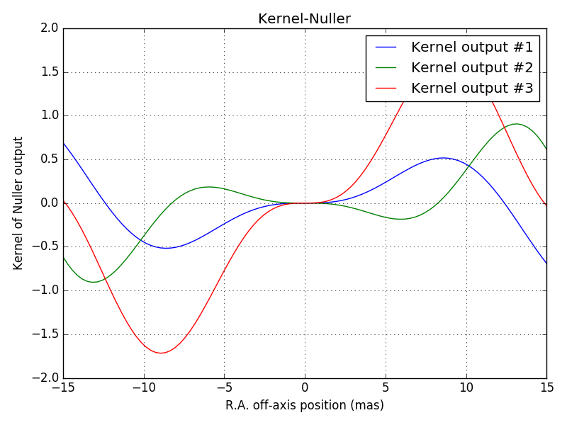
Figure 3: Evolution of the 3 kernels contained provided in Eq. 10 as a function of R.A. offset relative to the reference null (in milli-arcsecond). The vertical unit of the plot is in multiples of the transmission of a single telescope.

The kernel outputs that are are primary observables are then:

$$\mathbf{y}=\mathbf{K}\cdot\mathbf{x}.$$ (11)

Completing the description of the in-line interferometer introduced earlier, Figure 3 shows how the three kernels $\mathbf{y}$ vary as a function of the position of the target, as it moves across a $\pm$15 mas range of offset position relative to the null. The kernels consisting of linear combinations of anti-symmetric response curves are also anti-symmetric, just like closure- and kernel-phase.

Finally, we note that as our kernels are constructed as a linear combination of output intensities, they have the same properties whether phase noise occurs during an integration time or between integration times that are latter added in post-processing. This is in contrast to nonlinear techniques such as nulling self-calibration or closure-phase.

3 Properties of a kernel-nuller for VLTI

The high-contrast imaging properties of a nulling instrument, most notably the general shape of the on-sky transmission map, will depend on the exact location and size of the sub-apertures of the interferometer feeding light to the recombiner. While the method outlined above is infrastructure-agnostic, we will from now on examine at the special case of the VLTI, and describe the properties of a instrument concept called VIKiNG, an acronym standing for the VLTI Infrared Kernel NullinG instrument.

3.1 Practical Implementation

The direct detection of extrasolar planets with long baseline interferometry points towards the use of the L-band (3.4 - 4.1 $\mu$m) where the blackbody spectrum of forming planets is most likely to peak according to planet formation models, and that of mature planets kept warm by the proximity of their host star remains favorable. A viable practical implementation of both nulling and sensing functions as shown in Figure 1 could rely on multi-mode interference (MMI) couplers made of Chalcogenide glass (ChG) (Ma et al., 2013) that provide good bandwidth at very close to 50/50 coupling and realistic fabrication tolerances (Kenchington Goldsmith et al., 2017). Both functions could be integrated into one single photonic chip however fluctuations of the atmospheric thermal background will require some form of modulation. A bulk optics implementation, for instance inspired by Figure 2 of Guyon et al. (2013) may also be possible.

One of the technological difficulties in designing space-based nulling interferometers has been the ability to produce achromatic phase shifts and 50/50 couplers over large bandwidths. These problems do not go away in the kernel-nulling approach proposed here, but we note that the requirements are much more achievable for ground-based combiners aiming for the detection of warm exoplanets. For example, phase shifts need only be significantly better than the fringe tracking RMS, which is of order 100 nm for the best current fringe trackers. For a symmetrical physical nulling device such as the one represented by our nulling matrix $\mathbf{N}$, input geometric phase shifts between the inputs of $\pi$ are needed. A vacuum delay of 1.9 $\mu$m achieves a $\pi$ phase shift within 100nm for a 10% bandwidth in the astronomical L’ band at $\sim$3.8 $\mu$m, and simple first-order achromaticism with an air-glass combination easily improves this by a factor of 10. The combination of waveguide total length and core diameter can create similar achromaticity on a chip.

3.2 Nuller-output mapped on-sky

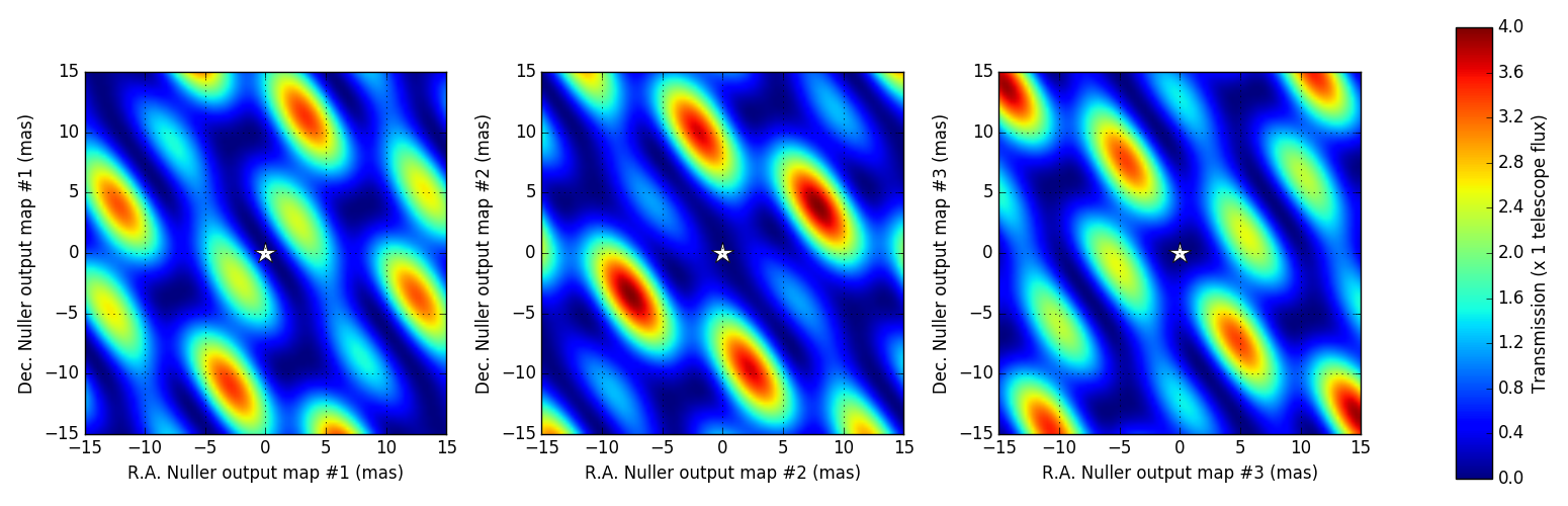
Figure 4: Transmission map for the three nulled outputs for a VLTI 4-UT aperture geometry over a $\pm$15 mas field of view. A five pointed star marks the location of the center of the field, where the rejection by the nuller is optimal. The three maps share the same colorbar, with a transmission that ranges from zero on the null to close to 100 % (4 $F_{T}$) for a few places in the field whose positions are dictated by the geometry of the interferometric array.

Table 2: VLTI Unit Telescope East and North coordinates (in meters)

Station	E	N
U1	-9.925	-20.335
U2	14.887	30.502
U3	44.915	66.183
U4	103.306	44.999

Our study case will focus on the simultaneous use of the four 8-meter diameter unit telescopes (UTs) of VLTI, pointing and cophased so as to observe a field of view conveniently located exactly at zenith. The coordinates for these stations, expressed in the reference system used to describe ESO’s Paranal observing facilities, are provided in Table 2. We start with the nuller introduced in Section 2.1 and described by the unitary matrix $\mathbf{N}$. It is used in the L-band at the wavelength $\lambda=3.6\,\mu\mathrm{m}$. For a snapshot observation, the field of view provided by the intererometer is given by the shortest (46.6 meter) baseline size of the array, corresponding to a $\sim$15 mas diameter.

In addition to the overall geometry of the array, the order by which the four input beams are recombined into the nuller will impact the imaging properties of the system. We will not attempt to optimize the nuller’s performance by re-ordering the input beams and will simply plug them in the order provided by Table 2. Figure 4 shows the resulting 2D transmission maps for each of the three outputs of the nuller over a $\pm$15 mas field of view both in right ascension and declination. The transmission is expressed in units of the flux collected by one aperture: $F_{T}$. As expected from the analysis of the in-line array, the three maps are symmetric about the origin: the transmission is zero on-axis, where the host-star would be located. The geometric arrangement of the four apertures makes the nuller observations, very much like any other interferometric observation, non-uniformly sensitive over the field. Each output features a different transmission profile that can peak up to close to 4 $F_{T}$ (corresponding to 100 % transmission) that is more sensitive to the presence of a structure for different parts of the field.

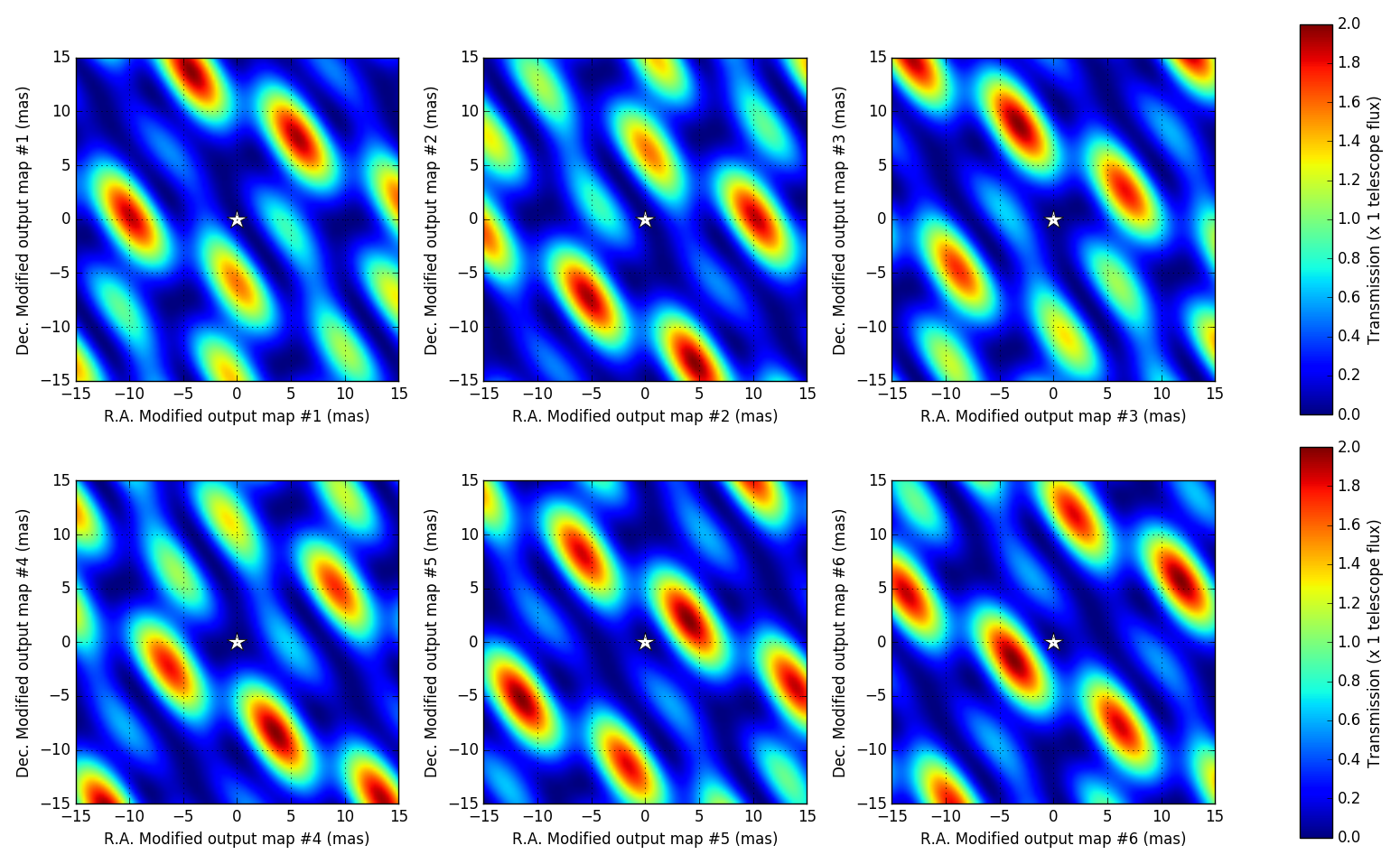
Figure 5: Transmission map for the six outputs of the modified nuller design for a VLTI 4-UT aperture geometry over a $\pm$15 mas field of view. A five pointed star marks the location of the center of the field, where the rejection by the nuller is optimal. All maps share the same colorbar, with a transmission that range from zero on the null to 50 % of the total flux collected by the four apertures (2 $F_{T}$). Compared to the maps provided in Figure 4, the amplitude of the colorscale was reduced by a factor of 2.

Figure 5 shows how the six transmission maps of the modified nuller vary over the same field of view. By doubling the number of outputs, one expects the flux per output to be reduced by a factor of two: the colorscale of the figure was therefore adjusted in consequence. The six new maps all have a significant anti-symmetric component about the center of the field, which means that in the absence of perturbation, these six observables can better constrain the position of a potential companion to an observed target.

Note that the sum of these six new transmission maps for the modified nuller, is identical to the sum of the three transmission maps of the original design: in the absence of coupling losses between the nulling and the mixing stages, the flux is simply redistributed amongst the different channels by the 3x6 combiner labeled $\mathbf{S}$ in Figure 1. This global transmission map is displayed in Figure 6: one can verify that it is the complement to the on-axis fringe pattern produced by the VLTI 4-UT array, rejected to the bright output of the nuller as illustrated in Fig. 1.

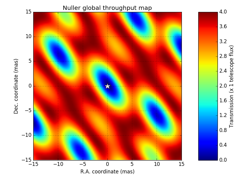
Figure 6: Map of the global throughput of the nuller, corresponding to the sum of the three maps provided in Fig. 4 or the six maps provided in Fig. 5.

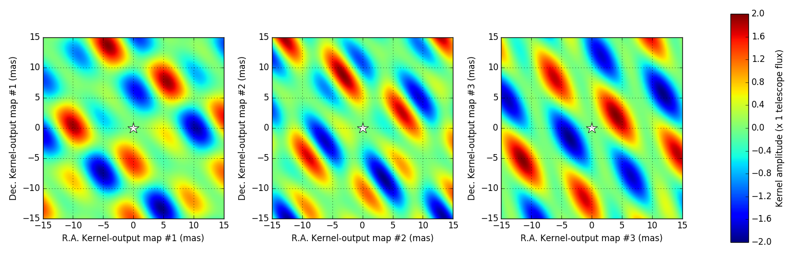
Figure 7: Evolution of the three kernel-outputs of the modified nuller architecture as a function of the position over a $\pm$15 mas field of view. Observe that all three maps are antisymmetric. The sign of the outputs can tell which side of the field of view a companion is.

3.3 Phase error robustness

We use the result of a series of simulated nulling observations that demonstrate the interest of the modified architecture and its kernel. As reminded by the different transmission maps used in the previous section, the detectability of an off-axis structure by the nuller is not uniform over the field of view. To ease our description, we will arbitrarily place a companion with a contrast $c=10^{-2}$ at the coordinates (+1.8, +4.8) mas in the system used so far, where the sensitivity of the nuller $\mathbf{N}$ is near optimal for the VLTI 4-UT (at zenith) configuration, as can be guessed by looking at the global throughput map shown in Figure 6.

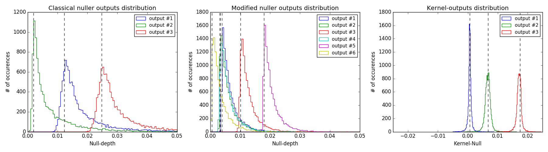
Figure 8: Distribution of the outputs of the nuller during the observation of a binary object (companion of contrast $c=10^{-2}$ at (+4.8, +1.8) mas) in the presence of 50 nm RMS residual piston excursions drawn from a normal distribution. From left to right: the nuller alone, the nuller+sensor and the kernels. The dashed lines mark the expected location of the different nulls (and their kernels) in the absence of piston excursion.

Figure 8 present the results of these simulations (a total of $10^{4}$ acquisitions per simulation), in the presence of 50 nm residual piston excursions. Each sub-figure features the histograms of outputs at the different stages of the concept. The null-depth bin values quoted in these figures are in units consistent with the transmission maps shown in Figures 4 and 5: the null-depth bin for a given output is proportional to the contrast of the companion, and multiplied by the transmission of the nuller for these coordinates.

The expected transmission of the three dark outputs after the 4x4 nulling-coupler is $t=(1.22,0.19,2.47)$. For a $c=10^{-2}$ contrast, one expects, in the absence of residual piston errors, outputs of 0.0122, 0.0019 and 0.0247, marked in the left panel of Figure 8 by three vertical dashed lines. In the presence of residual piston error, the distribution of observed null-depth deviates from what should be a Dirac distribution and evolves into the three plotted skewed distributions (see Hanot et al. (2011) for a formal model of this distribution). A real-world scenario with background and residual target shot-noise would convolve this distribution with a Gaussian, complicating its interpretation. The six outputs of the modified nuller design, including the mixing stage provided by $\mathbf{S}$ are similarly distributed, and are equally affected by the residual piston errors.

The raw nuller outputs spend very little time on the null and figuring out the true value of the null requires careful modeling of this distribution. By comparison, the kernel outputs, visible in the right panel of Figure 8, are well distributed and the statistics are relatively straightforward. Consistent with the general results from Ireland (2013), the uncertainty in the kernel outputs is proportional to the cube of the phase errors.

3.4 Sensitivity

For a companion of known relative position $(\alpha,\delta)$, the contrast $c$ is the solution to:

$$\mathbf{k}=\mathbf{m}\times c,$$ (12)

where $\mathbf{k}$ is a vector containing the measured three kernel-outputs ($\mathbf{y}$) normalised by the total flux (i.e. total including the starlight output) and $\mathbf{m}$ a vector containing the values of the kernel transmission maps (see Figure 7) for the coordinates $(\alpha,\delta)$. In the presence of uncertainties, the best estimate for $c$ is the least-square solution:

$$c=(\mathbf{m}^{T}\cdot\mathbf{k})/(\mathbf{m}^{T}\cdot\mathbf{m}),$$ (13)

with associated uncertainty:

$$\sigma_{c}=\frac{1}{|\mathbf{m}|}\sigma_{k},$$ (14)

where $\sigma_{y}$ is the dispersion of the kernel-output estimate. The $1/|\mathbf{m}|$ parameter scaling the two uncertainties depends on the position of the companion in the field of view, as shown in Figure 9, and varies from $\sigma_{c}=0.5\times\sigma_{k}$ in the most favorable configurations to $\sigma_{c}=10^{3}\times\sigma_{k}$ near the null, with a median ratio $\sigma_{c}=0.8\times\sigma_{k}$.

There are four key fundamental sources of uncertainty which are added in quadrature in forming the kernel-uncertainty $\sigma_{k}$: the fringe tracking phase errors ($\sigma_{k,\varphi}$), the cross-term between the fringe-tracking phase errors and intensity fluctuations on other telescopes ($\sigma_{k,I\varphi}$), the thermal background ($\sigma_{k,B}$) and the residual target photon noise ($\sigma_{k,T}$). For the uncertainty derived from the fringe-tracking phase, we can approximate the effect of many independent wavefront realizations by modeling the fringe-tracker uncertainty power spectrum as white up to a cutoff frequency $\Delta\nu_{\rm FT}$. This means that there are $\nu_{\rm FT}\times\Delta T$ realizations of fringe tracker errors, resulting in a contribution to the integrated kernel output uncertainty $\sigma_{k}$ of:

$$\sigma_{k,\varphi} \approx\sigma_{\varphi}^{3}\Delta\nu_{\rm FT}^{-1/2}\Delta T^{-1/2},$$ (15)

This equation becomes accurate at the $\sim$10 % level for $\sigma_{\varphi}<0.3$, which we have verified through simulation. Note that if the fringe tracker does not average to zero phase offset, then this third order kernel output uncertainty would not average to zero. In practice, any systematic offset in the fringe tracker zero point would have to be $\sim$10 times smaller than $\sigma_{\varphi}$ in order to be insignificant for typical exposure times and fringe tracker bandwidths. In the presence of precipitable water vapor, this stringent requirement can be achieved in different ways such as carrying out both nulling and fringe tracking at the same wavelength, fast re-calibration of the nulling setpoints (faster than water vapor seeing), or by dedicated control loops such as demonstrated with the KIN (Koresko et al., 2006) and the LBTI (Defrère et al., 2016).

The cross-term between intensity fluctuations and piston tracking errors is a second order term with a contribution to the kernel output uncertainty of:

$$\sigma_{k,I\varphi} \approx 2^{-1/2}\sigma_{\varphi}\sigma_{I}\Delta\nu_{\rm max}\Delta T^{-1/2},$$ (16)

where $\sigma_{I}$ is the intensity fluctuation on each telescope, and $\Delta\nu_{\rm max}$ is the maximum of the adaptive optics bandwidth (for fiber injection) and the piston bandwidth. From Jovanovic et al. (2017), practical RMS coupling efficiency variations with an extreme adaptive optics system can be of order 10% at 1.55 $\mu$m, which would correspond to $\sim$2% in the L’ band. Coupling fluctuations are often much worse than this for existing interferometers with adaptive optics, with one problem being inadequate control of low-order modes.

The contribution of residual target photon shot noise is:

$$\sigma_{k,T} \approx\sigma_{\varphi}^{2}F_{T}^{-1/2}\Delta T^{-1/2},$$ (17)

where $F_{T}$ is the target flux in photons/s/telescope, and other symbols are as before. The power of -1/2 is the combination of two terms: the $\sqrt{F_{T}}$ increase in the noise, and the scaling by $1/F_{T}$ in obtaining the normalised kernel outputs $\mathbf{k}$ from the raw outputs $\mathbf{y}$. The contribution of thermal background has a similar functional form for the same reason:

$$\sigma_{k,B} \approx F_{B}^{1/2}F_{T}^{-1}\Delta T^{-1/2}.$$ (18)

For observations in an L’ filter (3.4 to 4.1 $\mu$m), we can write (Tokunaga & Vacca, 2005) the target and background flux for a warm optics temperature of 290 K as:

$$F_{T} =3.5\times 10^{10}\eta_{c}\eta_{w}\left(\frac{D}{8\,{\rm m}}\right)^{2}10^{-0.4m_{L^{\prime}}}{\leavevmode\nobreak\ \rm photons/s}.$$ (19)

$$F_{B} =A(T_{w})\eta_{c}(1-\eta_{w}){\leavevmode\nobreak\ \rm photons/s}.$$ (20)

The background flux constant due to the warm telescope and interferometer optics $A(T_{w})$ per telescope is simply given by the Bose-Einstein distribution applicable to photons applied to two polarisations and one spatial mode. Note that this is the same as the Planck function in units of photons per unit frequency applied to an étendue of $\lambda^{2}$. This is $5.4\times 10^{7}$ photons/s for 290 K, and is generally given by:

$$A(T_{w}) =\frac{2\Delta\nu}{\exp(h\nu/k_{b}T_{w})-1},$$ (21)

for a filter central frequency $\nu$ and bandwidth $\Delta\nu$. With an assumption of warm optics efficiency of $\eta_{w}=0.25$, and a cold optics efficiency of $\eta=0.4$, the achievable contrast for 8 m telescopes is shown in Figure 10. These sensitivities are well within the range needed to detect a range of transiting exoplanets, exoplanets discovered by radial velocity and young, self-luminous exoplanets.

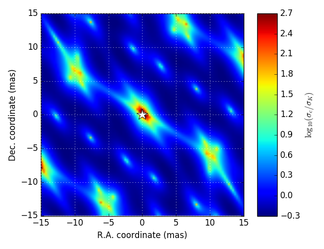
Figure 9: Map of the ratio between contrast uncertainty and kernel output uncertainty as a function of R.A. and Dec for the VLTI-4UT configuration. The map uses a logarithmic stretch, ranging from -0.3 ($\sigma_{c}=0.5\times\sigma_{k}$) in the most favorable configurations to $\sim$3 ($\sigma_{c}=10^{3}\times\sigma_{k}$) near the null. The median ratio is $\sigma_{c}=0.8\times\sigma_{k}$.

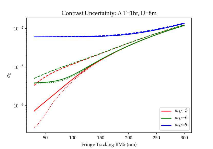
Figure 10: Contrast uncertainty (median over sky positions) as a function of fringe-tracker phase error, for different values of target magnitudes. Dotted line is for no intensity fluctuations, solid line for (realistic) 2% RMS intensity fluctuations and dashed line for poor 10% intensity fluctuations. For high target fluxes, fringe tracker phase error dominates, and for low target fluxes, thermal background dominates. Residual target shot noise never dominates at an optics temperature of 290 K.

3.5 The VIKiNG survey

The achievable contrast curves shown in Figure 10 suggest that even with a conservative 150 nm RMS fringe tracking performance, a contrast better than $c=10^{-5}$ can be achieved under realistic photometric stability conditions for targets brighter than $M_{L}=6$. A kernel-nulling observing campain using the four VLTI UTs therefore presents a real potential for the direct detection of nearby exoplanets discovered by radial velocity. To support this claim, we used the information compiled in the Extrasolar Planet Encyclopaedia database (exoplanet.eu) to select a sample of nearby known extrasolar planet hosts that would make valuable targets for our VIKiNG instrument concept, observing from VLTI at Paranal.

Selection criteria include a predicted contrast cutoff at $c=10^{-5}$, such that a maximum total observing time of two hours per target makes it possible to reach $SNR=5$, and an angular separation ranging from 5 to 15 mas. These conservative inner and outer working angles respectively correspond to the resolution of the longest and the shortest baselines for the assumed VLTI configuration. The outer working angle could be extended by taking into account the evolution of the (u,v) coverage over the observing time required to reach the required SNR.

Assuming that these objects are at thermal equilibrium with their host star allows to constrain a temperature (assuming albedo near zero, applicable to hot Jupiters). We also assume an intermediate Neptune-like density ($1.64g/cm^{3}$) for all planets and use M $\sin i$ to put a lower constraint on the planet radius. With temperature and radius estimates for both the star and the planet, we can predict a contrast, while a angular separation estimate is simply given by the ratio between the semi-major axis and the distance to the system. Fourteen targets fit all of the requirements. They are listed along with their predicted observational properties in Table 3.

Table 3: VIKiNG best targets

Planet	Separation	Contrast
name	(mas)	($\log_{10}{c}$)
GJ 86 A b	10	-4.03
BD+20 2457 b	7	-4.56
HD 110014 c	7	-4.56
11 Com b	12	-4.59
ksi Aql b	9	-4.61
61 Vir b	6	-4.67
HIP 105854 b	10	-4.68
HIP 107773 b	7	-4.75
HD 74156 b	5	-4.84
mu Ara c	6	-4.86
HD 168443 b	8	-4.87
HIP 67851 b	7	-4.91
HD 69830 b	6	-4.94
HD 16417 b	5	-4.99

The size of this sample doubles (Defrère et al., 2018b), if one assumes a tighter inner working angle of 1 mas ($0.25\times\lambda/B$), which brings in potentially warmer planets with more favorable contrasts. A more detailed characterization of the true VIKiNG discovery and characterization potential is beyond the scope of this paper that only aims at introducing a new instrument concept. It will likely be the object of future work, to be carried out in the context of the Hi-5 initiative (Defrère et al., 2018a).

4 Discussion

Lacour et al. (2014) proposed a different architecture concept for an interferometric nuller able to produce closure-phase measurements of nulled outputs. In the framework of this paper, the imaginary components of all three visibilities from those ABCD combiners are kernel outputs, and the imaginary component of the triple product simulated in that paper is just one of three robust observables. However, in the critical background-limited regime, using all three kernel-outputs in the combiner of Lacour et al. (2014) would require an exposure time 6 times larger than the architecture presented here (Figure 1). We have also argued here that a linear combination of outputs is adequate for high contrast imaging, without the need for the nonlinear operations of creating triple products or computing closure-phase.

It should also be observed that the methodology outlined earlier can also be applied to show that, the nulling observations are rendered robust against inter-beam intensity fluctuations, due either to high-altitude atmospheric turbulence (scintillation) or to intra-beam high-order wavefront aberrations that result in coupling losses. The null is also a quadratic function of these intensity fluctuations (Serabyn et al., 2012). While sensitive to photometric unbalance, the behavior of the nuller remains insensitive to global fluctuations of the source brightness. Like for the piston, with the flux of one sub-aperture taken reference, there are only six second-order relative perturbations terms that will impact the nuller’s outputs. The impact of these fluctuations can be modeled using the framework outlined for the phase, substituting in Equation 3, a real phase term $\varphi_{k}$ for an imaginary term, that results in an electric field with a modulus that deviates from unity. The structure of the resulting response matrix $\mathbf{A}$ is identical to the one for the phase: the same kernel matrix $\mathbf{K}$ will therefore simultaneously render the observable quantities robust against piston excursions and small amplitude photometric fluctuations: the uncertainty in the kernel-outputs is also proportional to the cube of the input complex amplitude fluctuations, so that even 10% intensity fluctuations on the inputs would translate into errors smaller than $10^{-3}$ on the kernel-outputs.

We have however reported that the coupling between fringe tracking errors and intensity fluctuations does contribute to the error budget as highlighted by Lay (2004). Our simulations suggest that under realistic (2 %) intensity fluctuations, these cross-terms do not significantly degrade our predicted performance.

5 Conclusion

High-contrast imaging solutions thus far implemented, either in the context of single-telescope coronagraphy or multi-aperture interferometry, have been conceived on the premiss of the optical subtraction of the static diffraction pattern produced by a stable on-axis source. The effective high-contrast detection potential of such static solutions is, in practice, severely limited by the least amount of wavefront perturbation that quickly drives otherwise near-ideal solutions away from their high-contrast reference point.

Drawing on the idea of kernel, here applied to the outputs of an interferometric nuller, we have described how the design of an otherwise plain four input beam interferometric nuller can be modified to take into account, the possibility of self-calibration. The result is a concept that, assuming good but no longer ideal observing conditions, becomes robust against residual wavefront aberrations (as well as photometric fluctuations), with errors dominated by third order input phase and intensity errors.

Kernel-nulling interferometry is a powerful idea: the architecture and method outlined in this paper make it possible to simultaneously benefit from the high-contrast boost provided by the nuller while keeping the ability to sense the otherwise degenerate effect of ever-changing observing conditions, so as to build observable quantities that are robust against those spurious effects. Similarly to closure-phase, our kernel-nulled outputs also break the symmetry degeneracy of a classical nuller’s output: the sign of the different kernels constrains which side of the field of view any asymmetric structure lies. Preliminary simulations suggest that under reasonable observing conditions, our VIKiNG instrument concept, using the four UTs of the VLTI infrastructure, could directly detect a dozen nearby planets discovered by radial velocity surveys, in less than two hours spent per target.

Note that with only four input beams, the special case described in this paper features a small number of possible covariance terms to keep track of. Future work will attempt to answer the questions: “Can the approach be further generalized and applied to situations where a large number of degrees of freedom are available?” and “How can a coronagraph be modified in order to benefit from similar properties?”

The proposed concept is of course not restricted to ground-based interferometry. The robustness boost brought by the concept of kernel-output reduces the otherwise demanding technological requirements on a space borne interferometer tasked with the direct detection of higher contrast ($10^{-10}$) Earth-like extrasolar planets. It would be valuable to brushup the original designs for the Darwin and TPF-I concept missions and see what a revised kernel-nulling architecture can bring.