First-order bifurcation detection for dynamic complex networks

Abstract

In this paper, we explore how network centrality and network entropy can be used to identify a bifurcation network event. A bifurcation often occurs when a network undergoes a qualitative change in its structure as a response to internal changes or external signals. In this paper, we show that network centrality allows us to capture important topological properties of dynamic networks. By extracting multiple centrality features from a network for dimensionality reduction, we are able to track the network dynamics underlying an intrinsic low-dimensional manifold. Moreover, we employ von Neumann graph entropy (VNGE) to measure the information divergence between networks over time. In particular, we propose an asymptotically consistent estimator of VNGE so that the cubic complexity of VNGE is reduced to quadratic complexity that scales more gracefully with network size. Finally, the effectiveness of our approaches is demonstrated through a real-life application of cyber intrusion detection.

Index Terms—  Bifurcation, centrality, graph Laplacian, von Neumann graph entropy, temporal network

1 Introduction

Many real-world complex systems ranging from physical systems, social media, financial markets and ecosystems to chemical reaction mechanisms are often represented as networks (or graphs) that possibly change over time [1, 2, 3, 4]. In a network representation, a set of elementary units, such as human, gene, sensor, or other types of ‘nodes’, are connected by ‘edges’ that describe relationships between nodes such as physical link, spatial vicinity, or friendship. Network representations allow us to explore structural properties of dynamic systems, and thus to study their behaviors, e.g., anomaly detection in cyber networks and community detection in social networks [5, 6]. In a dynamic system, there often exists a critical time instant at which the system shifts abruptly from one state to another. This critical threshold is associated with a first-order bifurcation [7] that occurs when a small change made to the system results in a sudden change of the system’s behavior. For example, a bifurcation of biological system was detected in the process of cell development when cells choose between two different fates [8, 9, 10, 11]. In this paper, we aim to explore how network-based approaches can be used in bifurcation detection.

Centrality measures provide important means of understanding the topological structure and dynamic process of complex networks [12]. Depending on the type of nodal influence to be emphasized, different centrality measures, such as degree, eigenvector, clustering coefficient, closeness and betweenness, are commonly used in the literature [1]. For example, degree centrality measures the total number of connections a node has, while eigenvector centrality implicitly measures the importance of a node by the importance of its neighbors. Network centrality allows us to capture multiple structural features from a single network, and thus expands the feature set for graph learning under limited network data samples. In this paper, we propose a spectral decomposition approach that integrates multiple network centrality features for graph learning. It is worth mentioning that our work is different from graph principal components analysis (PCA) [13, 14], where a graph Laplacian matrix was used to construct a smooth regularization function in PCA by assuming that the data manifold is encoded in the graph. In contrast to graph PCA, our approach finds the intrinsic low-dimensional manifold embedded in the centrality features. We show in this paper that the use of network centrality helps to identify differences in temporal networks.

In addition to network centrality, we employ von Neumann graph entropy (VNGE) to quantify the intrinsic network complexity. VNGE was originally introduced by [15], determined by the spectrum of the graph Laplacian matrix. It was shown in [16, 17, 18] that VNGE can measure the amount of information encoded in structural features of networks. For example, the entropy of random networks, e.g., Erdős-Rényi random graphs, is larger than the entropy of scale-free networks under the same average nodal degree [18, 19]. Compared to the existing graph entropy measures using notions of either randomness complexity or statistical complexity [20, 21], the main advantage of VNGE is its computational efficiency, leading to $O(n^{3})$ complexity in which $n$ is the network size. Here, we further improve the cubic complexity to $O(n^{2})$ by deriving a quadratic approximation to the VNGE. We show that such an approximation is asymptotically consistent, converging to the VNGE under mild conditions. Our experiments on a real-life application, cyber intrusion detection, demonstrate that the proposed approaches can efficiently track the structural changes of dynamic networks and identify bifurcation events.

2 Preliminaries: Graph Representation

A graph yields a succinct representation of interactions among nodes. Mathematically, we denote by $\mathcal{G}=(\mathcal{V},\mathcal{E},\mathbf{W})$ an undirected weighted graph, where $\mathcal{V}$ and $\mathcal{E}$ denote the node and edge sets with cardinality $|\mathcal{V}|=n$ and $|\mathcal{E}|=m$, and $\mathbf{W}\in\mathbb{R}^{n\times n}$ is a weighted matrix with entry $W_{ij}$ (or $[\mathbf{W}]_{ij}$) satisfying $W_{ij}=0$ if $i=j$ or $(i,j)\notin\mathcal{E}$. The quantitative study of $\mathcal{G}$ is often performed under its graph Laplacian matrix $\mathbf{L}=\mathbf{D}-\mathbf{W}$, where $\mathbf{D}=\operatorname{diag}(\mathbf{W}\mathbf{1})$ is the degree matrix. Here $\operatorname{diag}(\mathbf{a})$ denotes the diagonal matrix with diagonal vector $\mathbf{a}$, and $\mathbf{1}$ is the vector of all ones. It is known from spectral graph theory [22] that the second smallest eigenvalue of $\mathbf{L}$, called Fiedler number (FN), measures the network connectivity. And the number of zero eigenvalues of $\mathbf{L}$ gives the number of connected components of $\mathcal{G}$. Using the above notation, a dynamic network in a period of length $T$ can be represented as a sequence of graphs $\{\mathcal{G}_{t}\}_{t=1}^{T}$, where $\mathcal{G}_{t}=(\mathcal{V}_{t},\mathcal{E}_{t},\mathbf{W}_{t})$. Throughout the paper, we assume that the dynamic network contains the same set of nodes with $|\mathcal{V}_{t}|=|\mathcal{V}|=n$ for any $t$.

3 Network Diagnostics via Centrality Analysis

In this section, we introduce a graph diagnostic method that combines multiple centrality features to evaluate nodal importance to the network structure. By decomposing a single graph into multiple centrality features, we are able to achieve dimensionality reduction and feature decorrelation of the graph. We introduce several centrality measures of $\mathcal{G}$ that will be used in the sequel to define our feature set.

Degree (Deg) of node $i$ is defined as $\mathrm{Deg}(i)=L_{ii}=\sum_{j=1}^{n}W_{ij}$, where $\mathbf{L}$ is the graph Laplacian matrix.

Eigenvector centrality (Eig) is defined as the eigenvector of the adjacency matrix $\mathbf{W}$ associated with its largest positive eigenvalue $\lambda_{\max}$. The eigenvector centrality of node $i$ is given by $\mathrm{Eig}(i)=[\mathbf{v}]_{i}$ satisfying $\lambda_{\max}\mathbf{v}=\mathbf{W}\mathbf{v}$. Eigenvector centrality measures the importance of a node by the importance of its neighbors [1].

Local Fiedler vector centrality (LFVC) evaluates the impact of node removal on the network connectivity and partition [6]. LFVC of node $i$ is given by $\mathrm{LFVC}(i)=\sum_{j\in\{j|(i,j)\in\mathcal{E}\}}([\mathbf{f}]_{i}-[\mathbf{f}]_{j})^{2}$, where $\mathbf{f}$ is the eigenvector (known as Fiedler vector) of $\mathbf{L}$ associated with the smallest non-zero eigenvalue.

Closeness (Clos) is a global measure of geodesic distance of a node to all other nodes [23]. Let $\rho(i,j)$ denote the shortest path distance between node $i$ and node $j$ in a connected network. The closeness of node $i$ is defined as $\mathrm{Clos}(i)=\frac{1}{\sum_{j\in\mathcal{V},j\neq i}\rho(i,j)}$.

Betweenness (Betw) measures the fraction of shortest paths passing through a node relative to the total number of shortest paths in the network [24]. The betweenness of node $i$ is defined as $\mathrm{Betw}(i)=\sum_{{l\neq i}}\sum_{{j\neq i,j>l}}\frac{\phi_{lj}(i)}{\phi_{lj}}$, where $\phi_{lj}$ is the total number of shortest paths from node $l$ to $j$, and $\phi_{lj}(i)$ is the number of such shortest paths passing through node $i$.

Local clustering coefficient (LCC) quantifies how close a node’s neighbors are to become a complete graph [25]. LCC of node $i$ is given by $\mathrm{LCC}(i)=\frac{|\{(j,l)|j\in\mathcal{N}_{i},l\in\mathcal{N}_{i},(j,l)\in\mathcal{E}\}|}{|\mathcal{N}_{i}|(|\mathcal{N}_{i}|-1)/2}$, where $\mathcal{N}_{i}$ is the neighborhood set of node $i$.

Other topological features: The set of hop walk statistics is another useful network feature that takes into account indirect interactions among nodes. A node’s $h$-hop walk weight is given by the sum of edge weights associated with paths departing from this node and traversing through $h$ edges [26]. Moreover, given a set of reference nodes of interest, one can further expand the feature set by computing graph distances from reference nodes to other nodes [8].

Let $\mathbf{X}_{t}\in\mathbb{R}^{n\times p}$ denote the centrality-based feature matrix for a network at time $t$, where $n$ is the graph size, and $p$ is the number of centrality features. In contrast to graph PCA methods, which are often limited to undirected and connected graphs, our approach can be applied to directed and disconnected graphs. This is due to the fact that centrality features are also defined for directed and disconnected graphs. After acquiring the feature matrix $\mathbf{X}_{t}$, both linear and non-linear dimensionality reduction techniques [27] can be applied. As a result, we obtain a low-dimensional data representation $\mathbf{Y}_{t}\in\mathbb{R}^{n\times l}$ with $l\leq p$.

To better track the state of a dynamic network, we fit the data $\mathbf{Y}_{t}$ to a minimum volume ellipsoid (MVE), representing a certain confidence region for the state [28]. The MVE estimate at time $t$ can then be acquired by solving the convex program

$$\begin{array}[]{cl}\displaystyle\operatorname*{\text{minimize}}_{\mathbf{Q}\in\mathbb{R}^{l\times l},\mathbf{b}\in\mathbb{R}^{l}}&\det(\mathbf{Q}^{-1})\\ \operatorname*{\text{subject to}}&\|\mathbf{Q}\mathbf{y}_{i,t}-\mathbf{b}\|_{2}\leq 1,\leavevmode\nobreak\ i\in\mathcal{N}_{\alpha}\\ &\mathbf{Q}\succ 0,\end{array}$$ (4)

where $\mathbf{Q}$ and $\mathbf{b}$ are optimization variables, $\mathbf{y}_{i,t}^{T}$ denotes the $i$th row of $\mathbf{Y}_{t}$, and $\mathcal{N}_{\alpha}$ denotes the set of data within a $\alpha$ confidence region, determined by Mahalanobis distances of data below $\alpha=97.5\%$ quantile of the chi-square distribution with $l$ degrees of freedom [28]. The rationale behind problem (4) is that $\mathbf{P}\mathrel{\mathop{:}}=\mathbf{Q}^{2}$ and $\mathbf{c}\mathrel{\mathop{:}}=\mathbf{Q}^{-1}\mathbf{b}$ defines the ellipsoid $\{\mathbf{x}\in\mathbb{R}^{l}|(\mathbf{x}-\mathbf{c})^{T}\mathbf{P}(\mathbf{x}-\mathbf{c})\leq 1\}$, where the determinant of $\mathbf{P}$ (or $\mathbf{Q}$) is inversely proportional to the volume of this ellipsoid [29]. Since problem (4) involves a linear matrix inequality, it can be solved via semidefinite programming (SDP), e.g., the sdp solver in CVX [30]. The complexity of SDP is approximately of order $O(a^{2}b^{2}+ab^{3})$ [31], where $a$ and $b$ denote the number of optimization variables and the size of the semidefinite matrix, respectively. In (4), we have $a=l+(l+1)l/2$ and $b=l$, yielding the complexity $O(l^{6})$. Thanks to dimension reduction, problem (4) can be efficiently solved under a reduced feature space with small $l$.

4 von Neumann graph entropy

Von Neumann entropy (or quantum entropy) was originally used to measure the in-compressible information content of a quantum source, and can characterize the departure of a dynamical system from a pure state with zero entropy [16]. Recently, the von Neumann entropy of a graph, known as von Neumann graph entropy (VNGE), was used to efficiently measure the graph complexity [17]. By constructing a scaled graph Laplacian matrix $\mathbf{L}_{c}\mathrel{\mathop{:}}=c\mathbf{L}$ with $c=1/\mathrm{trace}(\mathbf{L})$, VNGE can be defined as [16, 18]

$$V=-\sum_{i=1}^{n}\lambda_{i}\log\lambda_{i},$$ (5)

where $\mathrm{trace}(\cdot)$ denotes the trace operator of a matrix, $\{\lambda_{i}\}_{i=1}^{n}$ are eigenvalues of $\mathbf{L}_{c}$, and the convention $0\log 0=0$ is used since $\lim_{x\to 0^{+}}x\log x=0$. It is clear from (5) that VNGE can be interpreted as the Shannon entropy of the probability distribution represented by $\{\lambda_{i}\}_{i=1}^{n}$ under the conditions that $\lambda_{i}\geq 0$ for any $i$ and $\sum_{i=1}^{n}\lambda_{i}=1$. Therefore, regular graphs with an uniform distribution of $\{\lambda_{i}\}_{i=1}^{n}$ provides an upper bound on VNGE. It was proved by [19] that the VNGE of Erdős-Rényi random graphs saturates this upper bound.

In (5), VNGE requires the full eigenspectrum of the graph Laplacian matrix, and thus has the cubic computational complexity $O(n^{3})$. In Proposition 1, we propose an approximate VNGE that scale more gracefully with the network size $n$.

Proposition 1

The quadratic approximation $\mathbf{Q}$ of VNGE $\mathbf{V}$ in (5) is given by

$$Q=1-c^{2}\left(\mathbf{d}^{T}\mathbf{d}+\mathbf{1}^{T}(\mathbf{W}\circ\mathbf{W})\mathbf{1}\right),$$ (6)

where $\mathbf{d}$ is the diagonal vector of $\mathbf{L}$, $\mathbf{W}$ is the weighted adjacency matrix, and $\circ$ denotes the entrywise product. Moreover,

$$Q\to\frac{V}{\log{n}},\quad n\to\infty,$$

when $n_{+}\sim n$ and $\lambda_{\max}\sim\lambda_{\min}$, where $n_{+}$ denotes the number of positive eigenvalues of $\mathbf{L}_{c}$, $\lambda_{\max}$ and $\lambda_{\min}$ denote the largest and smallest nonzero eigenvalues of $\mathbf{L}_{c}$, and for two functions $f(n)$ and $g(n)\neq 0$, $f(n)\sim g(n)$ means $\lim_{n\to\infty}f(n)/g(n)=1$.

Proof: See Proof in Sec. 7. $\blacksquare$

In contrast with (5), the quadratic approximation (6) yields an improved computational complexity of order $O(n^{2})$. Moreover, Proposition 1 implies that the asymptotic consistency of $Q$ with respect to $V$ is guaranteed up to a constant factor $\log{n}$. The condition $n_{+}\sim n$ implies that the number of disconnected components (given by $n-n_{+}$) is ultimately negligible compared to $n$. The condition $\lambda_{\max}\sim\lambda_{\min}$ implies that a graph Laplacian matrix has balanced eigenspectrum. This condition holds in regular and homogeneous random graph [18].

5 Experimental Results

(a)

(b)

Fig. 1: Centrality-based bifurcation detection. (a) MVEs of centrality features within $97.5\%$ confidence region. (b) $P$ value vs time.

In this section, we demonstrate the effectiveness of network centrality and VNGE in first-order bifurcation detection. We conduct our experiments using the UNB intrusion detection evaluation dataset [32, 26]. Here two graph sequences (with known adjacency matrices) are given in a time period of $6$ days, and each of them corresponds to a cyber network in which each node is a machine and an edge implies the presence of communication between machines. The first graph sequence describes the normal activity of cyber networks from day $1$ to day $6$. The second graph sequence includes abnormal networks under denial of service (DoS) and infiltrating attacks from day $4$ to day $6$.

In Fig. 1, we present principal component analysis based on network centrality features extracted from normal and abnormal networks. In Fig. 1-(a), we present MVEs that fits the 3D representations of network centrality features obtained from PCA. Here the trajectory of centroids is smoothed using the cubic spline. As we can see, there exists a divergence between the normal graph sequence and the abnormal graph sequence. The abrupt change from day $3$ to day $4$ reflects the anomalous behavior of the network after day $3$ when the attack began. The observed branching trajectory can be interpreted using the concept of bifurcation [7]: there exists a bifurcation of order $1$ in the sense that two simultaneous trends starting from the same type of networks (non-attacked) become separated from each other, toward two different types of networks (non-attacked versus attacked). In Fig. 1-(b), we evaluate the significance of the difference between the normal graph sequence and the abnormal graph sequence. Here the $P$ value is defined from the Hotelling’s T-squared test [33] associated with the null hypothesis that the centroids of ellipsoids from the normal and abnormal graph sequences are identical at a given time point. Clearly, day $4$ is the critical time for cyber intrusion with $P\text{ value}<0.01$.

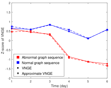
Fig. 2: VNGE of cyber networks over time.

In Fig. 2, we present VNGE of the studied two graph sequences, where VNGE is shown by its Z-score, which is normalized over time to have zero mean and unit variance. As we can see, the entropic pattern of the normal graph sequence is quite different from that of the abnormal sequence. Similar to Fig.,1, there exists a first-order bifurcation after day $3$. An interesting observation is that the VNGE of abnormal networks after bifurcation is lower than normal networks prior to bifurcation. That is because the network becomes more heterogeneous under attacks, e.g., DoS attack is accomplished by flooding some targeted machines with superfluous requests in an attempt to overload these hosts. And the VNGE decreases when the degree heterogeneity of a network increases [18, 16]. We further note that the approximate VNGE is close to the exact VNGE over time, implying the effectiveness of our proposed low-complexity approximation given by (6).

6 Conclusion

This paper showed how one can use network centrality and VNGE to detect bifurcation of dynamic complex networks. Network centrality enables us to capture important topological properties of dynamic networks, and VNGE provides an efficient approach to measure the information divergence between dynamic networks. When applied to cyber intrusion detection, our approaches effectively detected the network bifurcation event. In the future, we would like to delve into the relation between bifurcation and network entropy. We will also apply our approaches to other real-life applications.

7 Proof of Proposition 1

Based on Taylor series expansion of $\log x=\sum_{k=1}^{\infty}\frac{(-1)^{k-1}}{k}(x-1)^{k}$ at $x=1$, we have quadratic approximation

$$V\approx Q= -\sum_{i=1}^{n}\lambda_{i}(\lambda_{i}-1){=}1-\sum_{i=1}^{n}\lambda_{i}^{2}=1-\sum_{i=1}^{n}\sum_{j=1}^{n}[\mathbf{L}_{c}]_{ij}^{2}$$

$$\stackrel{{\scriptstyle(a)}}{{=}} 1-c^{2}\left(\sum_{i=1}^{n}L_{ii}^{2}+\sum_{i=1}^{n}\sum_{j\neq i}L_{ij}^{2}\right)=\text{\eqref{eq: VNGE_approx}},$$

where the equality $(a)$ holds due to the definition of $\mathbf{L}_{c}$ in (5), and $[\mathbf{A}]_{ij}$ (or $A_{ij}$) represents the $(i,j)$-th entry of a matrix $\mathbf{A}$. Assuming $\mathbf{L}_{c}$ has at least two nonzero eigenvalues, which implies $0<\lambda_{i}\leq\lambda_{\max}<1$ for any nonzero eigenvalue $\lambda_{i}$. We rewrite $V$ as

$$V=-\sum_{i:\lambda_{i}>0}\lambda_{i}\ln\lambda_{i}=-\sum_{i:\lambda_{i}>0}\lambda_{i}(1-\lambda_{i})\frac{\ln\lambda_{i}}{1-\lambda_{i}}.$$ (7)

Since for all $\lambda_{i}>0$, $\ln\lambda_{\min}\leq\ln\lambda_{i}\leq\ln\lambda_{\max}<0$ and $0<1-\lambda_{\max}\leq 1-\lambda_{i}\leq 1-\lambda_{\min}<1$, we obtain the relation

$$\frac{-\ln\lambda_{\max}}{1-\lambda_{\min}}\leq\frac{-\ln\lambda_{i}}{1-\lambda_{i}}\leq\frac{-\ln\lambda_{\min}}{1-\lambda_{\max}}.$$ (8)

Using $Q=\sum_{i=1}^{n}\lambda_{i}(1-\lambda_{i})=\sum_{i:\lambda_{i}>0}\lambda_{i}(1-\lambda_{i})$ and applying (8) to (7), we have

$$-Q\frac{\ln\lambda_{\max}}{1-\lambda_{\min}}\leq V\leq-Q\frac{\ln\lambda_{\min}}{1-\lambda_{\max}}.$$ (9)

Let $\lambda_{\max}=\frac{a}{n}$ and $\lambda_{\min}=\frac{b}{n}$ for some constants $a,b$ such that $a\geq b>0$. We obtain

$$\lim_{n\rightarrow\infty}-\frac{1}{\ln n}\cdot\frac{\ln\lambda_{\max}}{1-\lambda_{\min}}=\lim_{n\rightarrow\infty}\frac{1}{\ln n}\cdot\frac{\ln n-\ln a}{1-\frac{b}{n}}=1.$$

Similarly, $\lim_{n\rightarrow\infty}-\frac{1}{\ln n}\cdot\frac{\ln\lambda_{\min}}{1-\lambda_{\max}}=1$. Taking the limit of $\frac{V}{\ln n}$ and applying the above results into (9), we finally obtain $\lim_{n\rightarrow\infty}\frac{V}{\ln n}-Q=0$. $\blacksquare$

References

- [1] M. Newman, Networks: An Introduction, Oxford University Press, 2010.
- [2] Alexander Bertrand and Marc Moonen, “Seeing the bigger picture: How nodes can learn their place within a complex ad hoc network topology,” IEEE Signal Processing Magazine, vol. 30, no. 3, pp. 71–82, 2013.
- [3] A. Sandryhaila and J. M. F. Moura, “Big data analysis with signal processing on graphs: Representation and processing of massive data sets with irregular structure,” IEEE Signal Processing Magazine, vol. 31, no. 5, pp. 80–90, Sept. 2014.
- [4] P.-Y. Chen and K.-C. Chen, “Information epidemics in complex networks with opportunistic links and dynamic topology,” in IEEE Global Telecommunications Conference (GLOBECOM), 2010, pp. 1–6.
- [5] L. Akoglu, H. Tong, and D. Koutra, “Graph based anomaly detection and description: a survey,” Data Mining and Knowledge Discovery, vol. 29, no. 3, pp. 626–688, 2015.
- [6] P.-Y. Chen and A. O. Hero, “Deep community detection,” IEEE Transactions on Signal Processing, vol. 63, no. 21, pp. 5706–5719, 2015.
- [7] R. Borchert and N. A. Slade, “Bifurcation ratios and the adaptive geometry of trees,” Botanical Gazette, vol. 142, no. 3, pp. 394–401, 1981.
- [8] S. Liu, H. Chen, S. Ronquist, L. Seaman, N. Ceglia, W. Meixner, L. A. Muir, P.-Y. Chen, G. Higgins, P. Baldi, S. Smale, A. Hero, and I. Rajapakse, “Genome architecture leads a bifurcation in cell identity,” bioRxiv, 2017.
- [9] S. L. Spencer et al., “The proliferation-quiescence decision is controlled by a bifurcation in cdk2 activity at mitotic exit,” Cell, vol. 155, no. 2, pp. 369–383, 2013.
- [10] R. Bargaje, K. Trachana, M. N. Shelton, et al., “Cell population structure prior to bifurcation predicts efficiency of directed differentiation in human induced pluripotent cells,” Proceedings of the National Academy of Sciences, vol. 114, no. 9, pp. 2271–2276, 2017.
- [11] M. Scheffer, J. Bascompte, W. A. Brock, et al., “Early-warning signals for critical transitions,” Nature, vol. 461, no. 7260, pp. 53–59, 2009.
- [12] D. Wang, H. Wang, and X. Zou, “Identifying key nodes in multilayer networks based on tensor decomposition,” Chaos: An Interdisciplinary Journal of Nonlinear Science, vol. 27, no. 6, pp. 063108, 2017.
- [13] B. Jiang, C. Ding, and J. Tang, “Graph-laplacian pca: Closed-form solution and robustness,” in Proc. IEEE Conference on Computer Vision and Pattern Recognition, 2013, pp. 3492–3498.
- [14] N. Shahid, V. Kalofolias, X. Bresson, M. Bronstein, and P. Vandergheynst, “Robust principal component analysis on graphs,” in Proc. IEEE International Conference on Computer Vision, 2015, pp. 2812–2820.
- [15] S. L. Braunstein, S. Ghosh, and S. Severini, “The laplacian of a graph as a density matrix: a basic combinatorial approach to separability of mixed states,” Annals of Combinatorics, vol. 10, no. 3, pp. 291–317, 2006.
- [16] K. Anand, G. Bianconi, and S. Severini, “Shannon and von neumann entropy of random networks with heterogeneous expected degree,” Physical Review E, vol. 83, no. 3, pp. 036109, 2011.
- [17] L. Han, F. Escolano, E. R. Hancock, and R. C. Wilson, “Graph characterizations from von neumann entropy,” Pattern Recognition Letters, vol. 33, no. 15, pp. 1958–1967, 2012.
- [18] F. Passerini and S. Severini, “The von neumann entropy of networks,” arXiv, https://arxiv.org/abs/0812.2597, 2008.
- [19] W. Du, X. Li, Y. Li, and S. Severini, “A note on the von neumann entropy of random graphs,” Linear Algebra and its Applications, vol. 433, no. 11-12, pp. 1722–1725, 2010.
- [20] A. Torsello and E. R. Hancock, “Learning shape-classes using a mixture of tree-unions,” IEEE Transactions on Pattern Analysis and Machine Intelligence, vol. 28, no. 6, pp. 954–967, 2006.
- [21] D. P. Feldman and J. P. Crutchfield, “Measures of statistical complexity: Why?,” Physics Letters A, vol. 238, no. 4-5, pp. 244–252, 1998.
- [22] Fan RK Chung, Spectral graph theory, vol. 92, American Mathematical Soc., 1997.
- [23] G. Sabidussi, “The centrality index of a graph,” Psychometrika, vol. 31, no. 4, pp. 581–603, 1966.
- [24] L. C. Freeman, “A set of measures of centrality based on betweenness,” Sociometry, pp. 35–41, 1977.
- [25] D. J. Watts and S. H. Strogatz, “Collective dynamics of ‘small-world’networks,” nature, vol. 393, no. 6684, pp. 440–442, 1998.
- [26] P.-Y. Chen, S. Choudhury, and A. O. Hero, “Multi-centrality graph spectral decompositions and their application to cyber intrusion detection,” Proc. IEEE International Conference on Acoustics, Speech and Signal Processing (ICASSP), pp. 4553–4557, 2016.
- [27] L. Van Der Maaten, E. Postma, and J. Van den Herik, “Dimensionality reduction: a comparative,” J Mach Learn Res, vol. 10, pp. 66–71, 2009.
- [28] S. Van Aelst and P. Rousseeuw, “Minimum volume ellipsoid,” Wiley Interdisciplinary Reviews: Computational Statistics, vol. 1, no. 1, pp. 71–82, 2009.
- [29] P. Sun and R. M. Freund, “Computation of minimum-volume covering ellipsoids,” Operations Research, vol. 52, no. 5, pp. 690–706, 2004.
- [30] M. Grant, S. Boyd, and Y. Ye, “Cvx: Matlab software for disciplined convex programming,” 2008.
- [31] A. Nemirovski, “Interior point polynomial time methods in convex programming,” http://www2.isye.gatech.edu/~nemirovs/Lect_IPM.pdf.
- [32] A. Shiravi, H. Shiravi, M. Tavallaee, and A. A. Ghorbani, “Toward developing a systematic approach to generate benchmark datasets for intrusion detection,” computers & security, vol. 31, no. 3, pp. 357–374, 2012.
- [33] B. F. J. Manly and J. A. N. Alberto, Multivariate statistical methods: a primer, CRC Press, 2016.