Quantum phase transitions and the degree of nonidentity in the system with two different species of vector bosons

Abstract

We address the system with two species of vector bosons in an optical lattice. In addition to the the standard parameters characterizing such a system, we are dealing here with the “degree of atomic nonidentity”, manifesting itself in the difference of tunneling amplitudes and on-site Coulomb interactions. We obtain a cascade of quantum phase transitions occurring with the increase in the degree of atomic nonidentity. In particular, we show that the phase diagram for strongly distinct atoms is qualitatively different from that for (nearly) identical atoms considered earlier. The resulting phase diagrams evolve from the images similar to the “J. Miró-like paintings” to “K. Malewicz-like” ones.

I Introduction

Experimental research of ultracold atoms in optical lattices have dramatically expanded the possibilities of a tunable simulation of quantum many-body physics Greiner et al. (2002); Köhl et al. (2005); Kawaguchi and Ueda (2012); Hauke et al. (2012); Baier et al. (2016); Bermudez et al. (2017); Mazurenko et al. (2017). Moreover, ultracold atoms open the path to the parameter range that is hardly possible or even impossible to achieve in the natural condensed matter systems Meacher (1998); Jaksch et al. (1998); Grimm et al. (2000); Corboz et al. (2012).

The typical example is the system of vector bosons. This case corresponds to Bose–Hubbard model that is absent in the standard solid state theory Krutitsky (2016). The situation becomes even more intriguing, when the problem implies some additional nontrivial parameters. In our case, we have multiple vector boson species Belemuk et al. (2017). Then, in addition to the standard parameters, there appear nontrivial ones related to the “degree of atomic nonidentity”: the difference of tunneling amplitudes and on-site interactions.

Vector two-species bosons in optical lattices are characterized by the following parameters: hopping amplitudes $t_{\alpha}$, where $\alpha=1,2$ labels different bosons, $U_{\alpha,\alpha^{\prime}}$ — on-site interactions and spin-channel interaction parameters $U_{s}$ Krutitsky (2016); Belemuk et al. (2017). In recent paper, we have considered the simplest limiting case of nearly identical bosons Belemuk et al. (2017) in the Mott insulating state: $U_{12}\simeq U_{11}\simeq U_{22}=U_{0}$ and $t_{1}\simeq t_{2}\ll U_{0}$. This model differs from the case of perfectly identical bosons by the absence of cross-tunneling term: tunneling with the change of boson identity was forbidden. It has been shown in Belemuk et al. (2017) that the model can be reduced to the Kugel–Khomskii Kugel and Khomskii (1982) type spin–pseudospin model (where pseudospin labels different bosons). The assumption about perfectly identical bosons have lead to rather simple and intuitively expected phase diagram with one quantum phase transition near $U_{s}=0$ Belemuk et al. (2017).

Here, we investigate two species of cold vector bosons (ultacold bosonic atoms) in an optical lattice in the Mott insulating state ($U_{\alpha,\alpha^{\prime}}\gg|t_{\alpha}|$) and trace the evolution of the phase diagram with the increase in the degree of atomic nonidentity starting from nearly identical atoms. We show that nature of the ground states and the set of quantum phase transitions of sufficiently distinct atoms are qualitatively different from those in the case of (nearly) identical atoms considered earlier.

Actually, different ultra cold atoms in optical lattices have been considered in a number of papers in the last decade, see, e.g., Refs. Kuklov and Svistunov, 2003; Paredes et al., 2004; Isacsson et al., 2005; Mishra et al., 2007; Hubener et al., 2009; Takayoshi et al., 2010; Chung et al., 2012; Belemuk et al., 2014; Abanin et al., 2015; Belemuk et al., 2017; Potirniche et al., 2017; Penna and Richaud, 2017; Hu et al., 2018, and Refs. Georgescu et al., 2014; Dutta et al., 2015; Gross and Bloch, 2017 for review. Numerous striking effects induced by the multispecie nature of boson system have been found including quantum phase transitions, many-body localization, and topological order, as well as the superfluidity and supersolidity of ultracold atomic systems. However, most model investigations effectively deal with zero-spin boson species. Here, we focus on still unexplored physical phenomena in the systems with different species of vector bosons originating from the tunable interplay of spin degrees of freedom and of those identifying different sorts of atoms, see Fig. 1 for an illustration.

The rest of our paper is organized as follows: In Sec. II, we introduce the model Hamiltonian, then in Sec. III, we reduce the initial general Hamiltonian for vector bosons to the effective Hamiltonian appearing to be anisotropic spin-pseudospin model of the Kugel–Khomskii type Kugel and Khomskii (1982); in Sec. IV, we investigate different possible configurations in spin and pseudospin spaces and find their energy; in Sec. V, we discuss the energy of the ground state and the quantum phase transitions. In particular, in Sec. V, we illustrate the evolution of phase diagrams with the degree of atomic nonidentity, which looks like the transformation from the Joan Miró style artistic image to that of Kazimir Malewicz. Finally in Appendix, we present the analysis of several special limiting cases of the model Hamiltonian that relate our model system to some well-known results.

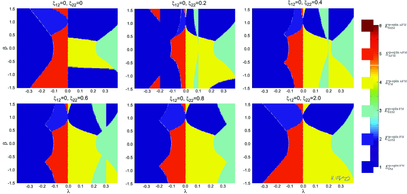
Figure 1: (Color online) Phase diagrams for $\xi_{12}=U_{12}/U_{11}=0$. Here $\beta=t_{2}/t_{1}$, $\xi_{22}=U_{22}/U_{11}$ and $\lambda=U_{s}/U_{11}$. In this case there is no Coulomb interaction between different atom kinds. The colorbar defines different spin and pseudospin orders.

II Hamiltonian for two species of vector bosons

We consider two types of boson atoms with $S=1$ in the optical lattice with sites labeled by index $i$. The corresponding creation operators $c^{\dagger}_{i\alpha s}$ where $s=\{-1,0,1\}$ is the spin index and $\alpha=1,2$ labels the type of the boson.

The Hamiltonian includes three terms:

$$H=H^{\scriptscriptstyle(U_{0})}+H^{\scriptscriptstyle(U_{s})}+H_{t}.$$ (1)

The interaction between bosons is given by two terms:

$$H^{\scriptscriptstyle(U_{0})}=\sum_{i}U_{12}n_{i,1}n_{i,2}+\frac{1}{2}\sum_{i,\alpha=1,2}U_{\alpha\alpha}n_{i,\alpha}(n_{i,\alpha}-1).$$ (2)

The first term corresponds to the repulsion between boson atoms at the same site Dutta et al. (2015). Here, $U_{11}$, $U_{22}$, and $U_{12}$ are three interaction parameters and $n_{i\alpha}=\sum_{s}c^{\dagger}_{i\alpha s}c_{i\alpha s}$. Now we assume that the interaction constants can strongly differ from each other, contrary to the case considered in Ref. Belemuk et al. (2017).

The spin-dependent interaction term is taken in the standard form Imambekov et al. (2003); Tsuchiya et al. (2004):

$$H^{\scriptscriptstyle(U_{s})}_{i}=U_{s}(\mathbf{S}_{i}^{2}-2n_{i})/2,$$ (3)

where $n_{i}=n_{i,1}+n_{i,2}$ is the total number of bosons at site $i$.

The hopping term

$$H_{t}=\sum_{\langle i,j\rangle}h_{t}\equiv\sum_{\langle i,j\rangle}t_{\alpha}\left(c^{\dagger}_{i\alpha\sigma}c_{j\alpha\sigma}+c^{\dagger}_{j\alpha\sigma}c_{i\alpha\sigma}\right),$$ (4)

where $\langle i,j\rangle$ means the summation only over the nearest-neighbor sites and $h_{t}$ is the hopping Hamiltonian for one link. As usual, the repeated indices imply summation.

In (4) and further on the spin variable is $\sigma$, whereas before the spin variable is defined as $s$.

III Effective Hamiltonian

Below we focus on the Mott insulating state, where cold atoms are localized at the sites of optical lattice with the number of bosons at each site equal to unity. We remind that in such case, the hopping terms (4) can be treated as perturbation compared to the interaction part of the Hamiltonian, $H^{\scriptscriptstyle(U_{0})}+H^{\scriptscriptstyle(U_{s})}$. Application of the perturbation theory reduces the initial general Hamiltonian to a simpler effective Hamiltonian written solely in terms of the spin and pseudospin (p-spin) operators related to the lattice sites with atom filling equal to one. These spin-1 $\mathbf{S}_{i}$ and p-spin-1/2 $\bm{\mathcal{T}}_{i}$ operators are defined in a standard way Yamashita et al. (1998)

$$S^{a}_{i}=c^{\dagger}_{i\alpha\sigma}s^{a}_{\sigma\sigma^{\prime}}c_{i\alpha\sigma^{\prime}},\qquad{\mathcal{T}}^{a}_{i}=c^{\dagger}_{i\alpha\sigma}\tau^{a}_{\alpha\beta}c_{i\beta\sigma},$$ (5)

where $a=x,y,z$.

Below we outline the algorithm of transforming the initial Hamiltonian to the effective one.

III.1 Basis states

In what follows, when we consider the link $\langle i,j\rangle$ between the nearest-neighbor sites, we focus on the basis of possible states for two bosons with spins $S_{1}=1$ and $S_{2}=1$ at neighboring sites $i=1$ and $j=2$. We are interested in the case with single occupation, i.e. when one boson of either type is located at each lattice site, $n_{i1}+n_{i2}=1$. We can pass now to the basis of the eigenstates of the total spin squared ${\bf S}^{2}=({\bf S}_{1}+{\bf S}_{2})^{2}$ and its $z$-projection $S^{z}=S^{z}_{1}+S^{z}_{2}$. We designate these states as $|SM\rangle$, $S=0,1,2$ and $M=-S,\ldots,S$. This basis can be written as follows

$$\Phi^{(f)}_{SM}=|\phi^{(f)}_{S}\rangle|SM\rangle,$$ (6)

where $f=1,\ldots,4$ enumerates the ways to distribute two types of bosons over two sites. The coordinate part $|\phi^{(f)}_{S}\rangle$ is given explicitly in Ref. Belemuk et al. (2017).

Applying $h_{t}$, see Eq. (4), to the basis states (6), we obtain two kinds of intermediate (virtual) states. The first type will be realized for two identical bosons at one site ($i$ or $j$), the second type is for two nonidentical bosons at one site. Intermediate energies depend on the spin and types of bosons. They are

$$E^{aa}_{S=0}=U_{11}-2U_{s},\quad E^{aa}_{S=2}=U_{11}+U_{s},$$

$$E^{bb}_{S=0}=U_{22}-2U_{s},\quad E^{bb}_{S=2}=U_{22}+U_{s},$$ (7)

$$E^{ab}_{S=0}=U_{12}-2U_{s},\quad E^{ab}_{S=2}=U_{12}+U_{s},$$

$$E^{ab}_{S=1}=U_{12}-U_{s}.$$

There are no intermediate states corresponding to the total spin $S=1$ for two identical $a$- or $b$-bosons due to the symmetry of the total wave function.

The energy of the virtual states with the double site occupancy is much larger than the energy of the states with the single site occupancy we are focusing at. To find corrections to the energy of the single-occupancy states related to the hoppings, we need the second order terms of the perturbation theory. So, further it will be convenient to work with the operator

$$h=-h_{\rm eff}=h_{t}(1/H_{0})h_{t},$$ (8)

where $H_{0}=H^{\scriptscriptstyle(U_{0})}+H^{\scriptscriptstyle(U_{s})}$. In the basis of states (6), the matrix of $h$ can be presented in the following block form

$$h=\begin{pmatrix}B_{11}&0&0&0\\ 0&B_{22}&B_{23}&0\\ 0&B_{32}&B_{33}&0\\ 0&0&0&B_{44}\end{pmatrix}.$$ (9)

The matrix $h$ here is in fact the block-matrix, where each block is $9\times 9$ matrix. Blocks $B_{kl}=\langle\Phi^{k}_{S^{\prime}M^{\prime}}|h|\Phi^{l}_{SM}\rangle$, $k,l=1,2,3,4$ are diagonal matrices. Their explicit forms are the following

$$B_{11}=4t_{1}^{2}\begin{pmatrix}\frac{1}{E^{aa}_{S=0}}I_{1}&\\ &0\cdot I_{3}&\\ &&\frac{1}{E^{aa}_{S=2}}I_{5}&\end{pmatrix},$$ (10)

$$B_{44}=4t_{2}^{2}\begin{pmatrix}\frac{1}{E^{bb}_{S=0}}I_{1}&\\ &0\cdot I_{3}&\\ &&\frac{1}{E^{bb}_{S=2}}I_{5}&\end{pmatrix},$$ (11)

$$B_{22}=B_{33}=(t_{1}^{2}+t_{2}^{2})\begin{pmatrix}\frac{1}{E^{ab}_{S=0}}I_{1}&\\ &\frac{1}{E^{ab}_{S=1}}I_{3}&\\ &&\frac{1}{E^{ab}_{S=2}}I_{5}&\end{pmatrix},$$ (12)

$$B_{23}=B_{32}=2t_{1}t_{2}\begin{pmatrix}\frac{1}{E^{ab}_{S=0}}I_{1}&\\ &\frac{1}{E^{ab}_{S=1}}I_{3}&\\ &&\frac{1}{E^{ab}_{S=2}}I_{5}&\end{pmatrix}.$$ (13)

Here $I_{n}$, $n=1,3,5$, are the identity $n\times n$ matrices. $I_{1}$ accounts for one state with $S=0$, $I_{3}$ accounts for three states with $S=1$, and $I_{5}$ accounts for five states with $S=2$.

In what follows, we identify the single occupancy of site $i$ with $a$- or $b$-boson by the pseudospin-$1/2$ states $|1\rangle_{i}=|+\rangle_{i}$ and $|2\rangle_{i}=|-\rangle_{i}$, respectively. It will be convenient to introduce explicitly two types of creation operators: $a^{\dagger}_{is}$ for bosons of type $\alpha=1$ and $b^{\dagger}_{is}$ for bosons of type $\alpha=2$.

For this purpose, we rewrite the pseudospin operator ${\mathcal{T}}^{\gamma}_{i}$ at sites $i$, see Eq. (5), in the form

$${\mathcal{T}}^{\gamma}_{i}=a^{\dagger}_{is}\tau^{\gamma}_{11}a_{is}+a^{\dagger}_{is}\tau^{\gamma}_{12}b_{is}+b^{\dagger}_{is}\tau^{\gamma}_{21}a_{is}+b^{\dagger}_{is}\tau^{\gamma}_{22}b_{is}.$$ (14)

We can rewrite, as usual, the set of $\mathcal{T}^{\gamma}$ operators in the other equivalent form:

$$T^{+}_{i}=a^{\dagger}_{is}b_{is},\quad T^{-}_{i}=b^{\dagger}_{is}a_{is},\quad T^{z}_{i}=\frac{1}{2}(a^{\dagger}_{is}a_{is}-b^{\dagger}_{is}b_{is}).$$

To describe the occupancy of sites $i$ and $j$, we introduce the basis of pseudospin states $|\alpha\beta\rangle=|\alpha\rangle_{i}|\beta\rangle_{j}$. Then, we find the correspondence between two-boson orbital states (6) and pseudospin states $|\alpha\beta\rangle$. For example, $|\phi^{(1)}_{S}\rangle\longrightarrow|++\rangle$.

In what follows, we map the matrix $h$, Eq. (9), onto an effective spin-pseudospin operator in the space $|\alpha\rangle_{i}|\beta\rangle_{j}|SM\rangle$. This operator will be given in terms of spin $S=1$ operators ${\bf S}_{i}$, ${\bf S}_{j}$ and pseudospin $T=1/2$ operators ${\bf T}_{i}$, ${\bf T}_{j}$ and it has the same structure as matrix $h$, Eq. (9).

Next, we introduce the projection operator $Q_{S}$ and $P_{T}$ onto the combination of states $|SM\rangle$ and $|TM_{T}\rangle$ corresponding to the total spin $S=0,1,2$ and pseudospin $T=0,1$ at the link $\langle i,j\rangle$. The projectors in the spin space $Q_{S}=\sum_{M=-S}^{S}|SM\rangle\langle SM|$ can be written as

$$Q_{0}=-\frac{1}{3}+\frac{1}{3}({\bf S}_{i}\cdot{\bf S}_{j})^{2},$$

$$Q_{1}=1-\frac{1}{2}({\bf S}_{i}\cdot{\bf S}_{j})-\frac{1}{2}({\bf S}_{i}\cdot{\bf S}_{j})^{2},$$ (15)

$$Q_{2}=\frac{1}{3}+\frac{1}{2}({\bf S}_{i}\cdot{\bf S}_{j})+\frac{1}{6}({\bf S}_{i}\cdot{\bf S}_{j})^{2},$$

where $Q_{0}+Q_{1}+Q_{2}=1$.

Similarly, in the pseudospin space the projectors onto the singlet $T=0$ and triplet $T=1$ states are

$$P_{s}=\frac{1}{4}-{\bf T}_{i}\cdot{\bf T}_{j},\quad P_{t}=\frac{3}{4}+{\bf T}_{i}\cdot{\bf T}_{j}.$$ (16)

It is also convenient to introduce the following projectors in the pseudospin space

$$P^{11} =|++\rangle\langle++|=\left(\frac{1}{2}+T^{z}_{i}\right)\left(\frac{1}{2}+T^{z}_{j}\right),$$

$$P^{22} =|+-\rangle\langle+-|=\left(\frac{1}{2}+T^{z}_{i}\right)\left(\frac{1}{2}-T^{z}_{j}\right),$$

$$P^{33} =|-+\rangle\langle-+|=\left(\frac{1}{2}-T^{z}_{i}\right)\left(\frac{1}{2}+T^{z}_{j}\right),$$ (17)

$$P^{44} =|--\rangle\langle--|=\left(\frac{1}{2}-T^{z}_{i}\right)\left(\frac{1}{2}-T^{z}_{j}\right),$$

and

$$P^{32}=|-+\rangle\langle+-|=T^{-}_{i}T^{+}_{j},$$ (18)

$$P^{23}=|+-\rangle\langle-+|=T^{+}_{i}T^{-}_{j}.$$

In addition, we use below the following identities:

$$P^{11}+P^{44} =\frac{1}{2}+2T^{z}_{i}T^{z}_{j},$$

$$P^{22}+P^{33} =\frac{1}{2}-2T^{z}_{i}T^{z}_{j},$$ (19)

$$P^{32}+P^{23} =2{\bf T}_{i}\cdot{\bf T}_{j}-2T^{z}_{i}T^{z}_{j}.$$

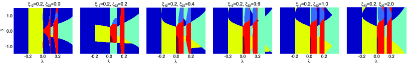
Figure 2: (Color online) Phase diagrams for small Coulomb interaction between different atom kinds: $\xi_{12}=U_{12}/U_{11}=0.2$. All the notations follow Fig. 1.

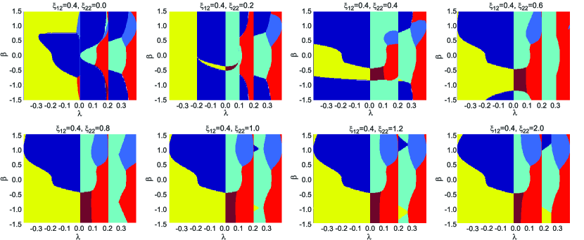
Figure 3: (Color online) Phase diagrams for $\xi_{12}=U_{12}/U_{11}=0.4$.

With the help of the projectors (15)–(18) and the identifie (19), we rewrite the block matrix $h$ in terms of spin and pseudospin operators as follows

$$h=4t_{1}^{2}{\,}P^{11}\left[\frac{Q_{0}}{E^{aa}_{0}}+\frac{Q_{2}}{E^{aa}_{2}}\right]+4t_{2}^{2}{\,}P^{44}\left[\frac{Q_{0}}{E^{bb}_{0}}+\frac{Q_{2}}{E^{bb}_{2}}\right]+(t_{1}^{2}+t_{2}^{2})\left[P^{22}+P^{33}\right]\left[\frac{Q_{0}}{E^{ab}_{0}}+\frac{Q_{1}}{E^{ab}_{1}}+\frac{Q_{2}}{E^{ab}_{2}}\right]+\\ +2t_{1}t_{2}\left[P^{23}+P^{32}\right]\left[\frac{Q_{0}}{E^{ab}_{0}}+\frac{Q_{1}}{E^{ab}_{1}}+\frac{Q_{2}}{E^{ab}_{2}}\right].$$ (20)

Substituting the explicit form of pseudospin projectors, we can rewrite $h$ in the form containing only spin projectors

$$h=\left\{\frac{t_{1}^{2}}{E^{aa}_{0}}+\frac{t_{2}^{2}}{E^{bb}_{0}}+2\left(\frac{t_{1}^{2}}{E^{aa}_{0}}-\frac{t_{2}^{2}}{E^{bb}_{0}}\right)(T^{z}_{i}+T^{z}_{j})+4\left(\frac{t_{1}^{2}}{E^{aa}_{0}}+\frac{t_{2}^{2}}{E^{bb}_{0}}\right)T^{z}_{i}T^{z}_{j}\right\}Q_{0}+\\ +\left\{\frac{t_{1}^{2}}{E^{aa}_{2}}+\frac{t_{2}^{2}}{E^{bb}_{2}}+2\left(\frac{t_{1}^{2}}{E^{aa}_{2}}-\frac{t_{2}^{2}}{E^{bb}_{2}}\right)(T^{z}_{i}+T^{z}_{j})+4\left(\frac{t_{1}^{2}}{E^{aa}_{2}}+\frac{t_{2}^{2}}{E^{bb}_{2}}\right)T^{z}_{i}T^{z}_{j}\right\}Q_{2}+\\ +\left\{\frac{1}{2}(t_{1}^{2}+t_{2}^{2})-2(t_{1}+t_{2})^{2}T^{z}_{i}T^{z}_{j}+4t_{1}t_{2}{\,}{\bf T}_{i}\cdot{\bf T}_{j}\right\}\left[\frac{Q_{0}}{E^{ab}_{0}}+\frac{Q_{1}}{E^{ab}_{1}}+\frac{Q_{2}}{E^{ab}_{2}}\right].$$ (21)

Finally, the effective Hamiltonian is written as the sum of $h$ operators (21) over all $\langle i,j\rangle$ links

$$H_{\rm eff}=-\sum\limits_{\langle i,j\rangle}h.$$ (22)

This is the most general form of the effective Hamiltonian involving different Hubbard interaction parameters, different hopping amplitudes, and spin-dependent interaction. In Appendix, we show that in a number of limiting cases, this Hamiltonian can be simplified to some well-known forms.

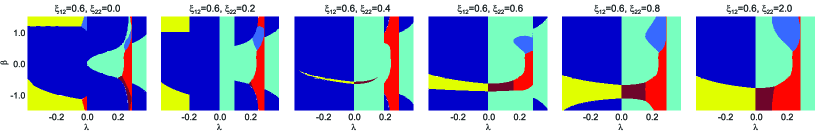
Figure 4: (Color online) Phase diagrams for $\xi_{12}=U_{12}/U_{11}=0.6$.

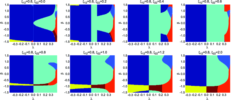
Figure 5: (Color online) Phase diagrams for $\xi_{12}=U_{12}/U_{11}=0.8$.

IV Energy of the ground state 

To proceed with the calculation of the ground state energy, we rewrite the “kernel” $h$ of effective Hamiltonian (22) as follows

$$h=\frac{2t_{1}^{2}}{U_{11}}\left(R_{0}Q_{0}+R_{2}Q_{2}+R_{1}\left[\frac{Q_{0}}{E_{0}^{ab}}+\frac{Q_{1}}{E_{1}^{ab}}+\frac{Q_{2}}{E_{2}^{ab}}\right]\right),$$ (23)

where the coefficients $R_{0}$, $R_{1}$ and $R_{2}$ are

$$R_{0}=\left[\frac{1}{2}\left(\frac{1}{E_{0}^{aa}}+\frac{\beta^{2}}{E_{0}^{bb}}\right)+\left(\frac{1}{E_{0}^{aa}}-\frac{\beta^{2}}{E_{0}^{bb}}\right)(T^{z}_{i}+T^{z}_{j})+\right.\\ \left.2\left(\frac{1}{E_{0}^{aa}}+\frac{\beta^{2}}{E_{0}^{bb}}\right)(T^{z}_{i}T^{z}_{j})\right],$$ (24)

$$R_{1}=\left[\frac{1}{4}(1+\beta^{2})-(1+\beta)^{2}(T^{z}_{i}T^{z}_{j})+2\beta({\bf T}_{i}\cdot{\bf T}_{j})\right],$$ (25)

$$R_{2}=\left[\frac{1}{2}\left(\frac{1}{E_{2}^{aa}}+\frac{\beta^{2}}{E_{2}^{bb}}\right)+\left(\frac{1}{E_{2}^{aa}}-\frac{\beta^{2}}{E_{2}^{bb}}\right)(T^{z}_{i}+T^{z}_{j})+\right.\\ \left.2\left(\frac{1}{E_{2}^{aa}}+\frac{\beta^{2}}{E_{2}^{bb}}\right)(T^{z}_{i}T^{z}_{j})\right].$$ (26)

Here, we introduce the dimensionless parameter $\beta=t_{2}/t_{1}$ that characterizes the difference of the tunnel amplitudes for different boson species.

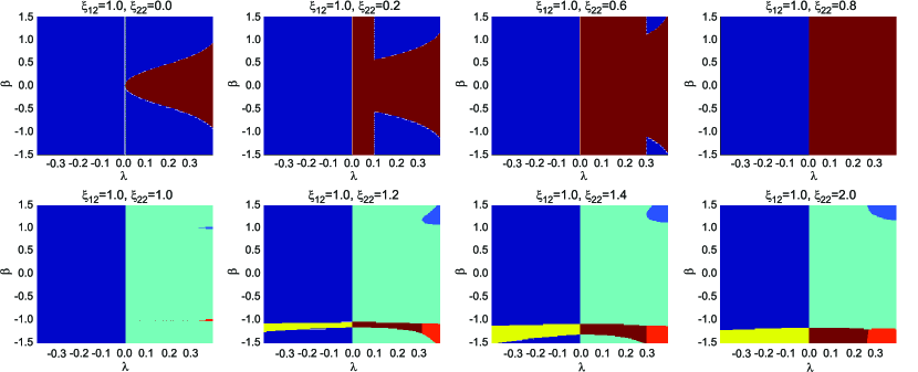
Figure 6: (Color online) Phase diagrams for $\xi_{12}=U_{12}/U_{11}=1.0$.

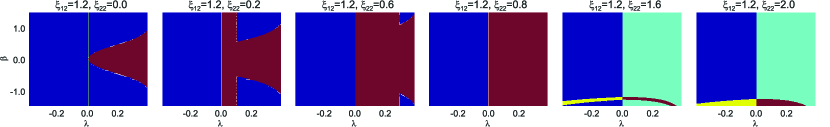
Figure 7: (Color online) Phase diagrams for $\xi_{12}=U_{12}/U_{11}=1.2$.

The energy $E$ of the ground state can be formally written as the average of the effective Hamiltonian over the ground state wave function (we will find it later using the variational approach)

$$E=-\frac{\nu}{2}\langle h\rangle,$$ (27)

where $\nu=2D$ is the number of nearest neighbors for the $D$-dimensional cubic lattice.

Within the mean-field approximation, we can neglect any correlations between spin and p-spin degrees of freedom. Then, for example, $\langle R_{0}Q_{0}\rangle\to\langle R_{0}\rangle\langle Q_{0}\rangle$, and

$$\langle h\rangle=E_{u}\left(\langle R_{0}\rangle\langle Q_{0}\rangle+\langle R_{2}\rangle\langle Q_{2}\rangle+\right.\\ \left.\langle R_{1}\rangle\left[\frac{\langle Q_{0}\rangle}{E_{0}^{ab}}+\frac{\langle Q_{1}\rangle}{E_{1}^{ab}}+\frac{\langle Q_{2}\rangle}{E_{2}^{ab}}\right]\right),$$ (28)

where $E_{u}=\frac{2t_{1}^{2}}{U_{11}}$.

We take the trial wave function in the p-spin space as the “mixed orbital state” on two-sublattices $A$ and $B$

$$|\chi\rangle_{i}=\cos\theta|+\rangle_{i}+\sin\theta|-\rangle_{i},\quad i\in A,$$ (29)

$$|\chi\rangle_{j}=\cos\theta|+\rangle_{j}+\eta\sin\theta|-\rangle_{j},\quad j\in B,\quad\eta=\pm 1.$$ (30)

For $\theta=0$, it defines the p-spin ferromagnetic (FM) state

$$|\uparrow_{i}\uparrow_{j}\uparrow_{i}\uparrow_{j}\dots\rangle.$$ (31)

For $\theta=\frac{\pi}{2}$, it defines also the p-spin FM state

$$|\downarrow_{i}(-\downarrow_{j})\downarrow_{i}(-\downarrow_{j})\dots\rangle.$$ (32)

The FM and antiferromagnetic (AFM) p-spin states will occur at $\theta=\frac{\pi}{4}$ for $\eta=+1$ and $\eta=-1$, respectively. These states are polarized in $x$ direction:

$$\frac{1}{\sqrt{2}}(|\uparrow\rangle+|\downarrow\rangle)_{i},$$ (33)

$$\frac{1}{\sqrt{2}}(|\uparrow\rangle+\eta|\downarrow\rangle)_{j}$$ (34)

For other angles $\theta$, the mixed orbital state is a some intermediate state between the FM and AFM ones. That is why, it is more correctly to refer to this mixed orbital state as the mixed orbital state with $\eta=+1$, or $\eta=-1$ rather than the FM and AFM states.

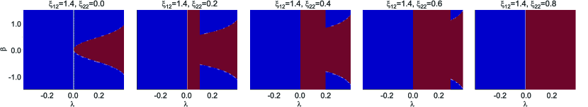
Figure 8: (Color online) Phase diagrams for $\xi_{12}=U_{12}/U_{11}=1.4$.

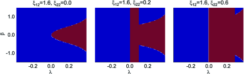
Figure 9: (Color online) Phase diagrams for $\xi_{12}=U_{12}/U_{11}=1.6$.

Now, we find averages over the trial mixed orbital state of the p-spin operators entering $R_{i}$, $i=0,1,2$

$$\langle T^{z}_{i}+T^{z}_{j}\rangle=\left\{\begin{aligned} &\cos 2\theta,\quad&\eta=+1,\\ &0,\quad&\eta=-1,\end{aligned}\right.$$ (35)

$$\langle T^{z}_{i}T^{z}_{j}\rangle=\left\{\begin{aligned} &\frac{1}{4}\cos^{2}2\theta,\quad&\eta=+1,\\ &-\frac{1}{4}\cos^{2}2\theta,\quad&\eta=-1,\end{aligned}\right.$$ (36)

$$\langle{\bf T}_{i}{\bf T}_{j}\rangle=\left\{\begin{aligned} &\frac{1}{4},\quad&\eta=+1,\\ &-\frac{1}{4},\quad&\eta=-1.\end{aligned}\right.$$ (37)

Later on, we will minimize the energy $E$ with respect to the angle $\theta$.

In contrast to the p-spin space, the effective Hamiltonian in the spin space is isotropic. So, we do not expect any exotic states there. Hence, we take for trial wave functions in the spin space the usual FM, AFM, and nematic (NEM) states Imambekov et al. (2003).

Then, the coefficients for projectors in the spin space are

$$\langle Q_{0}\rangle=\left\{\begin{aligned} &\,0\,,\quad\mathrm{FM},\\ &\frac{1}{3},\quad\mathrm{AFM},\\ &\frac{1}{3},\quad\mathrm{NEM},\end{aligned}\right.\qquad\langle Q_{1}\rangle=\left\{\begin{aligned} &\,0\,,\quad\mathrm{FM},\\ &\frac{1}{2},\quad\mathrm{AFM},\\ &\,0\,,\quad\mathrm{NEM},\end{aligned}\right.$$

$$\langle Q_{2}\rangle=\left\{\begin{aligned} &\,1\,,\quad\mathrm{FM},\\ &\frac{1}{6},\quad\mathrm{AFM},\\ &\frac{2}{3},\quad\mathrm{NEM}.\end{aligned}\right.$$ (38)

Finally, we have found all the averages and correlation functions entering Eq. (27) for the energy. We minimize numerically the energy $E(\theta,\eta)$, find the ground stats at different values of the parameters, and draw the corresponding phase diagrams.

V Results and discussion 

V.1 General properties of the phase diagrams

We address here the ground state of the system and possible quantum phase transitions. Performing the energy minimization, we find the phase diagrams for different ranges of the parameters. The key parameters are $\beta=t_{2}/t_{1}$, $\lambda=U_{s}/U_{11}$, $\xi_{12}=U_{12}/U_{11}$, and $\xi_{22}=U_{22}/U_{11}$. All these parameters (except $\lambda$ responsible for spin channel interaction) are related to the difference between the types of bosons.

There are six different phases: three phases have the ferromagnetic pseudospin arrangement, while three others correspond to the antiferromagnetic pseudospin state. Evolution of these phases is illustrated in Figs. 1–9; Fig. 1 is supplemented by the colorbar, where the correspondence between colors and phases is shown. Points at the colorbar correspond to the following orders in spin and pseudospin systems:

$$1 \rightarrow \operatorname{\mathit{E}^{p-spin\,\mathrm{\scriptscriptstyle{FM}}}_{\mathrm{\scriptscriptstyle{FM}}}}\,,$$

$$2 \rightarrow \operatorname{\mathit{E}^{p-spin\,\mathrm{\scriptscriptstyle{FM}}}_{\mathrm{\scriptscriptstyle{AFM}}}}\,,$$

$$3 \rightarrow \operatorname{\mathit{E}^{p-spin\,\mathrm{\scriptscriptstyle{FM}}}_{\mathrm{\scriptscriptstyle{NEM}}}}\,,$$ (39)

$$4 \rightarrow \operatorname{\mathit{E}^{p-spin\,\mathrm{\scriptscriptstyle{AFM}}}_{\mathrm{\scriptscriptstyle{FM}}}}\,,$$

$$5 \rightarrow \operatorname{\mathit{E}^{p-spin\,\mathrm{\scriptscriptstyle{AFM}}}_{\mathrm{\scriptscriptstyle{AFM}}}}\,,$$

$$6 \rightarrow \operatorname{\mathit{E}^{p-spin\,\mathrm{\scriptscriptstyle{AFM}}}_{\mathrm{\scriptscriptstyle{NEM}}}}\,.$$

Here, for example, color “1” corresponds to ferromagnetic spin and pseudospin orders.

In Figs. 1–9, we demonstrate the evolution of the phase diagrams within the wide range of parameters $\beta=t_{2}/t_{1}$, $\lambda=U_{s}/U_{11}$, $\xi_{12}=U_{12}/U_{11}$ and $\xi_{22}=U_{22}/U_{11}$. The most interesting phase transition is that accompanied by the change of atom distribution over the optical lattice: p-spin FM $\leftrightarrow$ p-spin AFM. Note that the cold colors correspond to FM p-spin, while the warm ones — to p-spin AFM. So the transitions with p-spin change can be found in the phase diagram at the lines, where cold colors change to warm ones.

Evolution of the phase diagrams for $\xi_{12}=U_{12}/U_{11}=0$ with $\xi_{22}=U_{22}/U_{11}$ on $(\lambda,\beta)$-plane is shown in Fig. 1. In this case, there is no Coulomb interaction between different boson species. We see that there is always quantum phase transition at the line $\lambda=0$. This is true not only for Fig. 1, but also for all phase diagrams in Figs. 1-9. This phase transition is driven by the sign change of spin channel interaction $U_{s}$. This transition has been recently revealed in Ref. Belemuk et al. (2017) for nearly identical vector bosons. Here, we show that this transition is very stable with respect to the evolution of the degree of nonidentity.

One can also see in Fig. 1, that the “left color” is always blue. It corresponds to FM spin ordering (with FM p-spin ordering). This situation is intuitively obvious: since the “left” phase is determined by large negative $\lambda$ — the interaction in the spin channel. In all the next figures, the “left color” also corresponds to the FM spin ordering, sometimes with the AFM p-spin ordering (yellow).

Looking through the complete set of phase diagrams, one can notice the absence of exact symmetry with the respect to reflections $\lambda\to-\lambda$ and $\beta\to-\beta$, though some traces are detectable. The $\beta$-symmetry is restored, when $\xi_{12}\gg\xi_{22}$.

Let us mention that the intuitive speculations useful, for example, in the case of simple Heisenberg model, can be misleading here, because the effective Hamiltonian is rather nontrivial.

We also underline the evolution of the artistic image of the phase diagrams. Namely, at small $\xi_{12}$ their style resembles the J. Miró paintings, while at large $\xi_{12}$ — those of K. Malewicz.

V.2 Phase diagrams: specific features

Figures 1–2 are the most multicolored — there are quantum phase transitions nearly between all the possible phases. These pictures correspond to the low or moderate interspecies Coulomb interaction $U_{12}$ as compared to the single-species one. This feature can be attributed to small or moderate difference in the parameters characterizing their nonidentity. One can also notice that there are many reentrant phase transitions in Figs. 1–9, especially for moderate $\xi_{12}$.

When $\xi_{22}$ becomes sufficiently large, then the nematic (NEM) spin phase prevails. The $\xi_{22}$-threshold for this behavior is the smallest at large $\xi_{12}$, as can be seen in Figs. 1–9.

VI Conclusions

To conclude, we have investigated the evolution of the quantum state of vector two-species bosons in optical lattices with the “degree of atomic nonidentity” that drives the cascade of quantum phase transitions. We have transferred the initial general Hamiltonian for vector bosons to the anisotropic spin-pseudospin model of the Kugel–Khomskii type that served as the effective Hamiltonian. The variational approach have been used to uncover the phase diagram of the system in hand. We have investigated also limiting cases of the effective Hamiltonian and demonstrated the relation of our rather complicated Hamiltonian to the well known results.

Appendix A Special cases of Hamiltonian (21)–(22)

We remind that $H_{\rm eff}=-\sum\limits_{\langle i,j\rangle}h$.

A.1 Equal Hubbard interaction parameters

Now, we take a look at more special cases. First we consider the case with equal Hubbard interaction parameters

$$U_{12}=U_{11}=U_{22}=U_{0}$$ (40)

Then

$$E^{ab}_{S}=E^{aa}_{S}=E^{bb}_{S}=E_{S},\qquad S=0,1,2,$$ (41)

and as follows from Eq. (21), the effective matrix $h$ reduces to the following form:

$$h=\frac{Q_{0}}{E_{0}}\left\{\frac{3}{2}(t_{1}^{2}+t_{2}^{2})+2(t_{1}^{2}-t_{2}^{2})(T^{z}_{i}+T^{z}_{j})+2(t_{1}-t_{2})^{2}{\,}T^{z}_{i}T^{z}_{j}+4t_{1}t_{2}{\,}{\bf T}_{i}\cdot{\bf T}_{j}\right\}+\\ +\frac{Q_{2}}{E_{2}}\left\{\frac{3}{2}(t_{1}^{2}+t_{2}^{2})+2(t_{1}^{2}-t_{2}^{2})(T^{z}_{i}+T^{z}_{j})+2(t_{1}-t_{2})^{2}{\,}T^{z}_{i}T^{z}_{j}+4t_{1}t_{2}{\,}{\bf T}_{i}\cdot{\bf T}_{j}\right\}+\\ +\frac{Q_{1}}{E_{1}}\left\{\frac{1}{2}(t_{1}^{2}+t_{2}^{2})-2(t_{1}+t_{2})^{2}{\,}T^{z}_{i}T^{z}_{j}+4t_{1}t_{2}{\,}{\bf T}_{i}\cdot{\bf T}_{j}\right\}$$ (42)

A.2 Equal Hubbard interaction parameters and equal hopping amplitudes

The effective matrix $h$ can be simplified further if one considers equal hopping amplitudes, $t_{1}=t_{2}=t$. For this case, as it can be seen from Eq. (42), matrix $h$ reduces to

$$h=\frac{Q_{0}}{E_{0}}\left\{3t^{2}+4t^{2}{\,}{\bf T}_{i}\cdot{\bf T}_{j}\right\}+\frac{Q_{2}}{E_{2}}\left\{3t^{2}+4t^{2}{\,}{\bf T}_{i}\cdot{\bf T}_{j}\right\}+\frac{Q_{1}}{E_{1}}\left\{t^{2}-8t^{2}{\,}T^{z}_{i}T^{z}_{j}+4t^{2}{\,}{\bf T}_{i}\cdot{\bf T}_{j}\right\}.$$ (43)

The last expression can be simplified if we take into account that

$$t^{2}-8t^{2}{\,}T^{z}_{i}T^{z}_{j}+4t^{2}{\,}{\bf T}_{i}\cdot{\bf T}_{j}=4t^{2}{\,}P_{t0},$$ (44)

where $P_{t0}=P_{t}-(P^{11}+P^{44})=\left[1/4-2T^{z}_{i}T^{z}_{j}+{\bf T}_{i}\cdot{\bf T}_{j}\right]$ is the projector onto the pseudospin state $|T=1,M_{T}=0\rangle$, when the the matrix $h$ can be reduced to the form

$$h=4t^{2}{\,}\left\{\frac{Q_{0}}{E_{0}}P_{t}+\frac{Q_{2}}{E_{2}}P_{t}+\frac{Q_{1}}{E_{1}}P_{t0}\right\}.$$ (45)

Note that due to the presence of the projector $P_{t0}$, the states with spin $S=1$ will be automatically symmetric in the orbital space, while the antisymmetric combination of orbital states is automatically excluded from the effective Hamiltonian.

Next, we rewrite the Hamiltonian $h$ in terms of the spin operators. We use the relation

$$-4t^{2}{\,}\left(\frac{Q_{0}}{E_{0}}+\frac{Q_{2}}{E_{2}}\right)=\left\{\frac{-4t^{2}}{3}\left(\frac{1}{E_{2}}-\frac{1}{E_{0}}\right)+\frac{-4t^{2}}{2E_{2}}{\,}{\bf S}_{i}\cdot{\bf S}_{j}+\frac{-4t^{2}}{3}\left(\frac{1}{E_{0}}+\frac{1}{2E_{2}}\right){\,}({\bf S}_{i}\cdot{\bf S}_{j})^{2}\right\}=\\ =\epsilon+J{\,}{\bf S}_{i}\cdot{\bf S}_{j}+K{\,}({\bf S}_{i}\cdot{\bf S}_{j})^{2},$$ (46)

where

$$J=\frac{-2t^{2}}{E_{2}},\quad K=\frac{-4t^{2}}{3}\left(\frac{1}{E_{0}}+\frac{1}{2E_{2}}\right),$$ (47)

$$\epsilon=\frac{-4t^{2}}{3}\left(\frac{1}{E_{2}}-\frac{1}{E_{0}}\right)=J-K.$$ (48)

Parameters $J$, $K$, and $\epsilon$ can be expressed explicitly via the initial interaction constants $U_{0}$ and $U_{s}$ as follows

$$J=\frac{-2t^{2}}{U_{0}+U_{s}},\quad K=\frac{-2t^{2}U_{0}}{(U_{0}+U_{s})(U_{0}-2U_{s})},$$ (49)

$$\epsilon=\frac{4t^{2}U_{s}}{(U_{0}+U_{s})(U_{0}-2U_{s})},$$ (50)

Now, the Hamiltonian takes the form

$$H_{\rm eff}=\sum\limits_{\langle i,j\rangle}\left\{\left[\epsilon+J{\,}{\bf S}_{i}\cdot{\bf S}_{j}+K{\,}({\bf S}_{i}\cdot{\bf S}_{j})^{2}\right]P_{t}+\left(\frac{-4t^{2}}{E_{1}}\right)Q_{1}P_{t0}\right\}.$$ (51)

Finally, the relation $P_{t}=P_{t0}+P^{11}+P^{44}$ and the definition of $Q_{1}$ (15) allows us to reduce the Hamiltonian to the form used in Ref. Belemuk et al. (2017),

$$H_{\rm eff}=\sum\limits_{\langle i,j\rangle}\Bigl{\{}\left[\epsilon+J{\,}{\bf S}_{i}\cdot{\bf S}_{j}+K{\,}({\bf S}_{i}\cdot{\bf S}_{j})^{2}\right](P^{11}+P^{44})+\left[\epsilon^{\prime}+J^{\prime}{\,}{\bf S}_{i}\cdot{\bf S}_{j}+K^{\prime}{\,}({\bf S}_{i}\cdot{\bf S}_{j})^{2}\right]{\,}P_{t0}\Bigr{\}},$$ (52)

where we introduced

$$J^{\prime}=2t^{2}\left(\frac{1}{E_{1}}-\frac{1}{E_{2}}\right),$$ (53)

$$K^{\prime}=\frac{-2t^{2}}{3}\left(\frac{2}{E_{0}}+\frac{1}{E_{2}}-\frac{3}{E_{1}}\right),$$ (54)

$$\epsilon^{\prime}=\frac{-4t^{2}}{3}\left(\frac{1}{E_{2}}-\frac{1}{E_{0}}+\frac{3}{E_{1}}\right).$$ (55)

A.2.1 One type of bosons

For the case of only one type of bosons, Hamiltonian (52) is equivalent to that of Ref. Yip (2003). For single type of bosons, the pseudospin operators become $c$-numbers: $T^{z}_{i}=\pm 1/2$, ${\bf T}_{i}\cdot{\bf T}_{j}$ should be replaced by $T^{z}_{i}T^{z}_{j}=1/4$, and projectors $P^{11}+P^{44}=1$, $P_{t0}=0$. Then Eq. (52) is reduced to the Hamiltonian considered in Ref. Yip (2003)

$$H_{\rm eff}=\sum\limits_{\langle i,j\rangle}\left\{\epsilon+J{\,}{\bf S}_{i}\cdot{\bf S}_{j}+K{\,}({\bf S}_{i}\cdot{\bf S}_{j})^{2}\right\}.$$ (56)

A.2.2 No spin-dependent interaction

If there is no spin-dependent interaction, i.e. $U_{s}=0$, then $E_{0}=E_{2}=E_{1}$ and $J=K=-2t^{2}/U_{0}$, $\epsilon=0$, $J^{\prime}=K^{\prime}=0$, and $\epsilon^{\prime}=-4t^{2}/U_{0}=2J$. The effective Hamiltonian, Eq. (52), is reduced to

$$H_{\rm eff}=J\sum\limits_{\langle i,j\rangle}\left\{2P_{t0}+\bigl{(}{\bf S}_{i}\cdot{\bf S}_{j}+({\bf S}_{i}\cdot{\bf S}_{j})^{2}\bigr{)}\left(P^{11}+P^{44}\right)\right\}.$$ (57)

And at last, if in this case, there is only one type of bosons, then $P_{t0}=0$, $P^{11}+P^{44}=1$, and the effective Hamiltonian describing effective interaction between identical bosons has the ferromagnetic character ($J<0$)

$$H_{\rm eff}=J\sum\limits_{\langle i,j\rangle}\left\{{\bf S}_{i}\cdot{\bf S}_{j}+({\bf S}_{i}\cdot{\bf S}_{j})^{2}\right\},\quad J=\frac{-2t^{2}}{U_{0}}.$$ (58)

The systems with identical bosons with odd and even number bosons per site were discussed in Refs. Imambekov et al. (2003); Tsuchiya et al. (2004).

References

- Greiner et al. (2002) M. Greiner, O. Mandel, T. Esslinger, T. W. Hänsch, and I. Bloch, Nature 415, 39 (2002).
- Köhl et al. (2005) M. Köhl, H. Moritz, T. Stöferle, K. Günter, and T. Esslinger, Phys. Rev. Lett. 94, 080403 (2005).
- Kawaguchi and Ueda (2012) Y. Kawaguchi and M. Ueda, Phys. Rep. 253, 253 (2012).
- Hauke et al. (2012) P. Hauke, F. M. Cucchietti, L. Tagliacozzo, I. Deutsch, and M. Lewenstein, Rep. Prog. Phys. 75, 082401 (2012).
- Baier et al. (2016) S. Baier, M. J. Mark, D. Petter, K. Aikawa, L. Chomaz, Z. Cai, M. Baranov, P. Zoller, and F. Ferlaino, Science 352, 201 (2016).
- Bermudez et al. (2017) A. Bermudez, L. Tagliacozzo, G. Sierra, and P. Richerme, Phys. Rev. B 95, 024431 (2017).
- Mazurenko et al. (2017) A. Mazurenko, C. S. Chiu, G. Ji, M. F. Parsons, M. Kanász-Nagy, R. Schmidt, F. Grusdt, E. Demler, D. Greif, and M. Greiner, Nature 545, 462 (2017).
- Meacher (1998) D. R. Meacher, Contemp. Phys. 39, 329 (1998).
- Jaksch et al. (1998) D. Jaksch, C. Bruder, J. I. Cirac, C. W. Gardiner, and P. Zoller, Phys. Rev. Lett. 81, 3108 (1998).
- Grimm et al. (2000) R. Grimm, M. Weidemuller, and Y. B. Ovchinnikov (Academic Press, 2000) pp. 95 – 170.
- Corboz et al. (2012) P. Corboz, M. Lajkó, A. M. Läuchli, K. Penc, and F. Mila, Phys. Rev. X 2, 041013 (2012).
- Krutitsky (2016) K. V. Krutitsky, Physics Reports Ultracold bosons with short-range interaction in regular optical lattices, 607, 1 (2016).
- Belemuk et al. (2017) A. M. Belemuk, N. M. Chtchelkatchev, A. V. Mikheyenkov, and K. I. Kugel, Phys. Rev. B 96, 094435 (2017).
- Kugel and Khomskii (1982) K. I. Kugel and D. I. Khomskii, Sov. Phys. - Uspekhi 25, 231 (1982).
- Kuklov and Svistunov (2003) A. B. Kuklov and B. V. Svistunov, Phys. Rev. Lett. 90, 100401 (2003).
- Paredes et al. (2004) B. Paredes, A. Widera, V. Murg, O. Mandel, S. Fölling, I. Cirac, G. V. Shlyapnikov, T. W. Hänsch, and I. Bloch, Nature 429, 277 (2004).
- Isacsson et al. (2005) A. Isacsson, M.-C. Cha, K. Sengupta, and S. M. Girvin, Phys. Rev. B 72, 184507 (2005).
- Mishra et al. (2007) T. Mishra, R. V. Pai, and B. P. Das, Phys. Rev. A 76, 013604 (2007).
- Hubener et al. (2009) A. Hubener, M. Snoek, and W. Hofstetter, Phys. Rev. B 80, 245109 (2009).
- Takayoshi et al. (2010) S. Takayoshi, M. Sato, and S. Furukawa, Phys. Rev. A 81, 053606 (2010).
- Chung et al. (2012) C.-M. Chung, S. Fang, and P. Chen, Phys. Rev. B 85, 214513 (2012).
- Belemuk et al. (2014) A. M. Belemuk, N. M. Chtchelkatchev, and A. V. Mikheyenkov, Phys. Rev. A 90, 023625 (2014).
- Abanin et al. (2015) D. A. Abanin, W. De Roeck, and F. m. c. Huveneers, Phys. Rev. Lett. 115, 256803 (2015).
- Potirniche et al. (2017) I.-D. Potirniche, A. C. Potter, M. Schleier-Smith, A. Vishwanath, and N. Y. Yao, Phys. Rev. Lett. 119, 123601 (2017).
- Penna and Richaud (2017) V. Penna and A. Richaud, Phys. Rev. A 96, 053631 (2017).
- Hu et al. (2018) S. Hu, T. Wang, A. Pelster, S. Eggert, and X. Zhang, Bulletin of the American Physical Society (2018).
- Georgescu et al. (2014) I. Georgescu, S. Ashhab, and F. Nori, Rev. Mod. Phys. 86, 153 (2014).
- Dutta et al. (2015) O. Dutta, M. Gajda, P. Hauke, M. Lewenstein, D.-S. Luhmann, B. A. Malomed, T. Sowinski, and J. Zakrzewski, Rep. Prog. Phys. 78, 066001 (2015).
- Gross and Bloch (2017) C. Gross and I. Bloch, Science 357, 995 (2017), http://science.sciencemag.org/content/357/6355/995.full.pdf .
- Imambekov et al. (2003) A. Imambekov, M. Lukin, and E. Demler, Phys. Rev. A 68, 063602 (2003).
- Tsuchiya et al. (2004) S. Tsuchiya, S. Kurihara, and T. Kimura, Phys. Rev. A 70, 043628 (2004).
- Yamashita et al. (1998) Y. Yamashita, N. Shibata, and K. Ueda, Phys. Rev. B 58, 9114 (1998).
- Yip (2003) S. K. Yip, Phys. Rev. Lett. 90, 250402 (2003).