The Geodesic Farthest-point Voronoi Diagram in a Simple Polygon

Abstract

Given a set of point sites in a simple polygon, the geodesic farthest-point Voronoi diagram partitions the polygon into cells, at most one cell per site, such that every point in a cell has the same farthest site with respect to the geodesic metric. We present an $O(n\log\log n+m\log m)$-time algorithm to compute the geodesic farthest-point Voronoi diagram of $m$ point sites in a simple $n$-gon. This improves the previously best known algorithm by Aronov et al. [Discrete Comput. Geom. 9(3):217-255, 1993]. In the case that all point sites are on the boundary of the simple polygon, we can compute the geodesic farthest-point Voronoi diagram in $O((n+m)\log\log n)$ time.

1 Introduction

Let $P$ be a simple polygon with $n$ vertices. For any two points $x$ and $y$ in $P$, the geodesic path $\pi(x,y)$ is the shortest path contained in $P$ connecting $x$ with $y$. Note that if the line segment connecting $x$ with $y$ is contained in $P$, then $\pi(x,y)$ is a line segment. Otherwise, $\pi(x,y)$ is a polygonal chain whose vertices (other than its endpoints) are reflex vertices of $P$. The geodesic distance between $x$ and $y$, denoted by $d(x,y)$, is the sum of the Euclidean lengths of the line segments in $\pi(x,y)$. Throughout this paper, when referring to the distance between two points in $P$, we mean the geodesic distance between them unless otherwise stated. We refer the reader to the survey by Mitchell [12] in the handbook of computational geometry for more information on geodesic paths and distances.

Let $S$ be a set of $m$ point sites contained in $P$. For a point $x\in P$, a (geodesic) $S$-farthest neighbor of $x$, is a site $\textsc{n}(P,S,x)$ (or simply $\textsc{n}(x)$) of $S$ that maximizes the geodesic distance to $x$. To ease the description, we assume that every vertex of $P$ has a unique $S$-farthest neighbor. This general position condition was also assumed by Aronov et al. [3] and Ahn et al. [2].

The geodesic farthest-point Voronoi diagram of $S$ in $P$ is a subdivision of $P$ into Voronoi cells. Imagine that we decompose $P$ into Voronoi cells $\mathsf{Cell}(S,s)$ (or simply $\mathsf{Cell}(s)$) for each site $s\in S$, where $\mathsf{Cell}(S,s)$ is the set of points in $P$ that are closer to $s$ than to any other site of $S$. Note that some cells might be empty. The set $P\setminus\cup_{s\in S}\mathsf{Cell}(s)$ defines the (farthest) Voronoi tree of $S$ with leaves on the boundary of $P$. Each edge of this diagram is either a line segment or a hyperbolic arc [3]. The Voronoi tree together with the set of Voronoi cells defines the geodesic farthest-point Voronoi diagram of $S$ (in $P$), denoted by $\mathsf{FVD}[S]$ (or simply $\mathsf{FVD}$ if $S$ is clear from context). We indistinctively refer to $\mathsf{FVD}$ as a tree or as a set of Voronoi cells.

There are similarities between the Euclidean farthest-point Voronoi diagram and the geodesic farthest-point Voronoi diagram (see [3] for further references). In the Euclidean case, a site has a nonempty Voronoi cell if and only if it is extreme, i.e., it lies on the boundary of the convex hull of the set of sites. Moreover, the clockwise sequence of Voronoi cells (at infinity) is the same as the clockwise sequence of sites along the boundary of the convex hull. With these properties, the Euclidean farthest-point Voronoi diagram can be computed in linear time if the convex hull of the sites is known [1]. In the geodesic case, a site with nonempty Voronoi cell lies on the boundary of the geodesic convex hull of the sites. The order of sites along the boundary of the geodesic convex hull is the same as the order of their Voronoi cells along the boundary of $P$. However, the cell of an extreme site may be empty, roughly because the polygon is not large enough for the cell to appear. In addition, the complexity of the bisector between two sites can be linear in the complexity of the polygon.

Previous Work.

Since the early 1980s many classical geometric problems have been studied in the geodesic setting. The problem of computing the geodesic diameter of a simple $n$-gon $P$ (and its counterpart, the geodesic center) received a lot of attention from the computational geometry community. The geodesic diameter of $P$ is the largest possible geodesic distance between any two points in $P$, and the geodesic center of $P$ is the point of $P$ that minimizes the maximum geodesic distance to the points in $P$.

Chazelle [5] gave the first algorithm for computing the geodesic diameter of $P$, which runs in $O(n^{2})$ time using linear space. Suri [17] reduced the time complexity to $O(n\log n)$ without increasing the space complexity. Later, Hershberger and Suri [9] presented a fast matrix search technique, one application of which is a linear-time algorithm for computing the diameter of $P$.

The first algorithm for computing the geodesic center of $P$ was given by Asano and Toussaint [4], and runs in $O(n^{4}\log n)$ time. This algorithm computes a super set of the vertices of $\mathsf{FVD}[V]$, where $V$ is the set of vertices of $P$. In 1989, Pollack et al. [16] improved the running time to $O(n\log n)$. In a recent paper, Ahn et al. [2] settled the complexity of this problem by presenting a $\Theta(n)$-time algorithm to compute the geodesic center of $P$.

The problem of computing the geodesic farthest-point Voronoi diagram is a generalization of the problems of computing the geodesic center and the geodesic diameter of a simple polygon. For a set $S$ of $m$ points in $P$, Aronov et al. [3] presented an algorithm to compute $\mathsf{FVD}[S]$ in $O(n\log n+m\log m)$ time. While the best known lower bound is $\Omega(n+m\log m)$, which is a lower bound known for computing the geodesic convex hulls of $S$, it is not known whether or not the dependence on $n$, the complexity of $P$, is linear in the running time. In fact, this problem was explicitly posed by Mitchell [12, Chapter 27] in the Handbook of Computational Geometry.

Our Result.

In this paper, we present an $O(n\log\log n+m\log m)$-time algorithm for computing $\mathsf{FVD}[S]$ for a set $S$ of $m$ points in a simple $n$-gon. To do this, we present an $O((n+m)\log\log n)$-time algorithm for the simpler case that all sites are on the boundary of the simple polygon and use it as a subprocedure for the general algorithm.

Our result is the first improvement on the computation of geodesic farthest-point Voronoi diagrams since 1993 [3]. It partially answers the question posed by Mitchell. Moreover, our result suggests that the computation time of Voronoi diagrams has only almost linear dependence in the complexity of the polygon. We believe our results could be used as a stepping stone to solve the question posed by Mitchell [12, Chapter 27]. Indeed, after the preliminary version [14] of this paper had been presented, Oh and Ahn [13] presented an $O(n+m\log m+m\log^{2}n)$-time algorithm for this problem. They observed that the adjacency graph of the Voronoi cells has complexity smaller than the complexity of the Voronoi diagram and presented an algorithm for the geodesic farthest-point Voronoi diagram based on a polygon-sweep paradigm, which is optimal for a moderate-sized point-set.

Outline.

We first assume that the site set is the vertex set of the input simple polygon. Then we present an algorithm for computing $\mathsf{FVD}[S]$, which will be extended to handle the general cases in Section 6 and Section 7. This algorithm consists of three steps. Each section from Section 3 to Section 5 describes a step of the algorithm. In the first step, we compute the geodesic farthest-point Voronoi diagram restricted to the boundary of the polygon. In the second step, we decompose recursively the interior of the polygon into smaller cells, not necessarily Voronoi cells, until the complexity of each cell becomes constant. In the third step, we explicitly compute the geodesic farthest-point Voronoi diagram in each cell and merge them to complete the description of the Voronoi diagram.

In the first step, we compute the restriction of $\mathsf{FVD}[S]$ to $\partial P$ in linear time, where $\partial P$ denotes the boundary of $P$. A similar approach was used by Aronov et al. [3]. However, their algorithm spends $\Theta(n\log n)$ time and uses completely different techniques. The main tool used to speed up the algorithm is the matrix search technique introduced by Hershberger and Suri [9] which provides a “partial” description of $\mathsf{FVD}[S]\cap\partial P$ (i.e., the restriction of $\mathsf{FVD}[S]$ to the vertices of $P$.) To extend it to the entire boundary of $P$, we borrow some tools used by Ahn et al. [2]. This reduces the problem to the computation of upper envelopes of distance functions which can be completed in linear time.

In the second step, we recursively subdivide the polygon into cells. To subdivide a cell whose boundary consists of $t$ geodesic paths, we construct a closed polygonal path that visits roughly $\sqrt{t}$ endpoints of the $t$ geodesic paths at a regular interval. Intuitively, to choose these endpoints, we start at the endpoint of a geodesic path on the boundary of the cell. Then, we walk along the boundary, choose another endpoint after skipping $\sqrt{t}$ of them, and repeat this. We consider the geodesic paths, each connecting two consecutive chosen endpoints. The union of all these geodesic paths can be computed in time linear in the complexity of the cell [15] and subdivides the cell into smaller simple polygons. By recursively applying this procedure on each resulting cell, we guarantee that after $O(\log\log n)$ rounds the boundary of each cell consists of a constant number of geodesic paths. While decomposing the polygon, we also compute $\mathsf{FVD}[S]$ restricted to the boundary of each cell. However, the total complexity of $\mathsf{FVD}[S]$ restricted to the boundary of each cell might be $\omega(n)$ in the worst case. To resolve this problem, we subdivide each cell further so that the total complexity of $\mathsf{FVD}[S]$ restricted to the boundary of each cell is $O(n)$ for every iteration. Each round can be completed in linear time, which leads to an overall running time of $O(n\log\log n)$. After the second step, we have $O(n\log\log n)$ cells in the simple polygon and we call them the base cells.

In the third step, we explicitly compute the geodesic farthest-point Voronoi diagram in each of the base cells by applying the linear-time algorithm of computing the abstract Voronoi diagram given by Klein and Lingas [11]. To apply the algorithm, we define a new distance function for each site whose Voronoi cell intersects the boundary of each cell $T$ such that the distance function is continuous on $T$ and the total complexity of the distance functions for all sites is $O(n)$. We show that the abstract Voronoi diagram restricted to a base cell $T$ is exactly the geodesic farthest-point Voronoi diagram restricted to $T$. After computing the geodesic farthest-point Voronoi diagrams for every base cell, they merge them to complete the description of the Voronoi diagram.

For the case that the sites lie on the boundary of the simple polygon, we cannot apply the matrix searching technique directly although the other procedures still work. To handle this, we apply the matrix search technique with a new distance function to compute $\mathsf{FVD}[S]$ restricted to the vertices of $P$. Then we consider the general case that the sites are allowed to lie in the interior of the simple polygon. We subdivide the input simple polygon in a constant number of subpolygons, and apply the previous algorithm for sites on the boundary to these subpolygons. The overall strategy is similar to the one for sites on the boundary, but there are a few nontrivial technical issues to be addressed.

2 Preliminaries

For any subset $A$ of $P$, let $\partial A$ and $\mathrm{int}(A)$ denote the boundary and the interior of $A$, respectively. For any two points $x,y\in\mathbb{R}^{2}$, we use $xy$ to denote the line segment connecting $x$ and $y$. Let $P$ be a simple $n$-gon and $S$ be a set of $m$ point sites contained in $P$. Let $V$ be the set of the vertices of $P$. A vertex $v$ of a simple polygon is convex (or reflex) if the internal angle at $v$ with respect to the simple polygon is less than (or at least) $\pi$.

For any two points $x$ and $y$ on $\partial P$, let $\partial P[x,y]$ denote the portion of $\partial P$ from $x$ to $y$ in clockwise order. We say that three (nonempty) disjoint sets $A_{1},A_{2}$ and $A_{3}$ contained in $\partial P$ are in clockwise order if $A_{2}\subset\partial P[a,c]$ for any $a\in A_{1}$ and any $c\in A_{3}$. To ease notation, we say that three points $x,y,z\in\partial P$ are in clockwise order if $\{x\},\{y\}$ and $\{z\}$ are in clockwise order.

2.1 Ordering Lemma

Aronov et al. [3] gave the following lemma which they call Ordering Lemma. We make use of this lemma to compute $\mathsf{FVD}$ restricted to $\partial P$. Before introducing the lemma, we need to define the geodesic convex hull of a set $S$ of $m$ points in $P$. We say a subset $A$ of $P$ is geodesically convex if $\pi(x,y)\subseteq A$ for any two points $x,y\in A$. The geodesic convex hull of $S$ is defined to be the intersection of all geodesic convex sets containing $S$. It can be computed in $O(n+m\log m)$ time [8]. .

Lemma 1 ([3, Corollary 2.7.4]).

The order of sites along $\partial\mathsf{CH}$ is the same as the order of their Voronoi cells along $\partial P$, where $\mathsf{CH}$ is the geodesic convex hull of $S$ with respect to $P$.

2.2 Apexed Triangles

An apexed triangle $\triangle=(a,b,c)$ with apex $\textsc{a}(\triangle)=a$ is an Euclidean triangle contained in $P$ with an associated distance function $g_{\triangle}(x)$ such that (1) $\textsc{a}(\triangle)$ is a vertex of $P$, (2) there is an edge of $\partial P$ containing both $b$ and $c$, and (3) there is a site $\textsc{d}(\triangle)$ of $S$, called the definer of $\triangle$, such that

$$g_{\triangle}(x)=\begin{cases}\|x-\textsc{a}(\triangle)\|+d(\textsc{a}(\triangle),\textsc{d}(\triangle))=d(x,\textsc{d}(\triangle))&\text{if $x\in\triangle$}\\ -\infty&\text{if $x\notin\triangle$},\end{cases}$$

where $\|x-y\|$ denote the Euclidean distance between $x$ and $y$.

Intuitively, $\triangle$ bounds a constant complexity region where the geodesic distance function from $\textsc{d}(\triangle)$ can be obtained by looking only at the distance from $\textsc{a}(\triangle)$. We call the side of an apexed triangle $\triangle$ opposite to the apex the bottom side of $\triangle$. Note that the bottom side of $\triangle$ is contained in an edge of $P$.

The concept of the apexed triangle was introduced by Ahn et al. [2] and was a key to their linear-time algorithm to compute the geodesic center. After computing the $V$-farthest neighbor of each vertex in linear time [9], they show how to compute $O(n)$ apexed triangles in $O(n)$ time with the following property: for each point $p\in P$, there exists an apexed triangle $\triangle$ such that $p\in\triangle$ and $\textsc{d}(\triangle)=\textsc{n}(P,V,p)$. By the definition of the apexed triangle, we have $d(p,\textsc{n}(P,V,p))=g_{\triangle}(p)$. In other words, the distance from each point of $P$ to its $V$-farthest neighbor is encoded in one of the distance functions associated with these apexed triangles.

More generally, we define a set of apexed triangles whose distance functions encode the distances from the points of $P$ to their $S$-farthest neighbors. We say a weakly simple polygon $\gamma$ is a funnel of a point $p\in P$ if its boundary consists of three polygonal curves $\partial P[u,v]$, $\pi(u,p)$ and $\pi(v,p)$ for some two points $u,v\in\partial P$.

Definition 2.

A set of apexed triangles covers $\mathsf{FVD}[S]$ if for any site $s\in S$, the union of all apexed triangles with definer $s$ is a funnel $\gamma_{s}$ of $s$ such that $\mathsf{Cell}(S,s)\subset\gamma_{s}$.

Ahn et al. [2] gave the following lemma. In Section 6 and Section 7, we show that we can extend this lemma to compute a set of apexed triangles covering $\mathsf{FVD}[S]$ for any set $S$ of points in a simple polygon.

Lemma 3 ([2]).

Given a simple $n$-gon $P$ with vertex set $V$, we can compute a set of $O(n)$ apexed triangles covering $\mathsf{FVD}[V]$ in $O(n)$ time.

While Lemma 3 is not explicitly stated by Ahn et al. [2], a closer look at the proofs of Lemmas 5.2 and 5.3, and Corollaries 6.1 and 6.2 reveals that this lemma holds. Lemma 3 states that for each vertex $v$ of $P$, the set of apexed triangles with definer $v$ forms a connected component. In particular, the union of their bottom sides is a connected chain along $\partial P$. Moreover, these apexed triangles are interior disjoint by the definition of apexed triangles.

2.3 The Refined Geodesic Farthest-point Voronoi Diagram

Assume that we are given a set of $O(n+m)$ apexed triangles covering $\mathsf{FVD}[S]$. We consider a refined version of $\mathsf{FVD}[S]$ which we call the refined geodesic farthest-point Voronoi diagram defined as follows: for each site $s\in S$, the Voronoi cell $\mathsf{Cell}(s)$ of $\mathsf{FVD}[S]$ is subdivided by the apexed triangles with definer $s$. That is, for each apexed triangle $\triangle$ with definer $s$, we define a refined cell $\mathsf{rCell}(\triangle)=\triangle\cap\mathsf{Cell}(s)$, where $\triangle$ is the union of $\mathrm{int}(\triangle)$ and its bottom side (excluding the corners of $\triangle$). Since any two apexed triangles $\triangle_{1}$ and $\triangle_{2}$ with the same definer are interior disjoint, $\mathsf{rCell}(\triangle_{1})$ and $\mathsf{rCell}(\triangle_{2})$ are also interior disjoint. We denote the set $P\setminus\cup_{\triangle}\mathsf{rCell}(\triangle)$ by $\mathsf{rFVD}$. Then, $\mathsf{rFVD}$ forms a tree consisting of arcs and vertices. Notice that each arc of $\mathsf{rFVD}$ is a part of either the bisector of two sites or a side of an apexed triangle. Since we assume that the number of the apexed triangles is $O(n+m)$, the complexity of $\mathsf{rFVD}$ is still $O(n+m)$. (Lemma 2.8.3 in [3] shows that the complexity of $\mathsf{FVD}$ is $O(n+m)$.)

Lemma 4.

For an apexed triangle $\triangle$ and a point $x$ in $\mathsf{rCell}(\triangle)$, the line segment $xy$ is contained in $\mathsf{rCell}(\triangle)$, where $y$ is the point on the bottom side of $\triangle$ hit by the ray from $\textsc{a}(\triangle)$ towards $x$.

Proof.

Let $p$ be a point on $xy$. We have $d(\textsc{d}(\triangle),p)=d(\textsc{d}(\triangle),x)+d(x,p)$. On the other hand, $d(s,p)\leq d(s,x)+d(x,p)$ by the triangle inequality for any site $s$. Since $d(s,x)<d(\textsc{d}(\triangle),x)$ for any site $s$ other than $\textsc{d}(\triangle)$, we have $d(s,p)<d(\textsc{d}(\triangle),p)$, which implies that $p$ lies in $\mathsf{rCell}(\triangle)$. ∎

Corollary 5.

For any site $s\in S$ and any point $x\in\mathsf{Cell}(s)$, the line segment $xy$ is contained in $\mathsf{Cell}(s)$, where $y$ is the point on $\partial P$ hit by the ray from the neighbor of $x$ along $\pi(s,x)$ towards $x$.

Throughout this paper, we use $|C|$ to denote the number of edges of $C$ for a simple polygon $C\subseteq P$. For a curve $\gamma$, we use $|\mathsf{rFVD}\cap\gamma|$ to denote the number of the refined cells intersecting $\gamma$. For ease of description, we abuse the term ray slightly such that the ray from $x\in P$ in a direction denotes the line segment $xy$ of the halfline from $x$ in the direction, where $y$ is the first point of $\partial P$ encountered along the halfline from $x$.

From Section 3 to Section 5, we will make the assumption that $S$ is the set of the vertices of $P$. This assumption is general enough as we show how to extend the result to the case when $S$ is an arbitrary set of sites contained in $\partial P$ (Section 6) and in $P$ (Section 7). The algorithm for computing $\mathsf{FVD}[V]$ consists of three steps. Each section from Section 3 to Section 5 describes each step.

3 Computing $\mathsf{FVD}$ Restricted to $\partial P$

Using the algorithm in [2], we compute a set $\mathcal{A}$ of $O(n)$ apexed triangles covering $\mathsf{FVD}[S]=\mathsf{FVD}[V]$ in $O(n)$ time. Recall that the apexed triangles with the same definer are interior disjoint and have their bottom sides on $\partial P$ whose union forms a connected chain along $\partial P$. Thus, such apexed triangles can be sorted along $\partial P$ with respect to their bottom sides.

Lemma 6.

Given a set $\tau_{s}$ of all apexed triangles of $\mathcal{A}$ with definer $s$ for a site $s$ of $S$, we can sort the apexed triangles in $\tau_{s}$ along $\partial P$ with respect to their bottom sides in $O(|\tau_{s}|)$ time.

Proof.

The bottom side of an apexed triangle is contained in an edge of $\partial P$, and the other two sides are chords of $P$ (possibly flush with $\partial P$). Assume that these chords are oriented from its apex to its bottom side. Using a hash-table storing the chords of the apexed triangles in $\tau_{s}$, we can link each of these chords to its neighboring triangles (and distinguish between left and right neighbors). In this way, we can retrieve a linked list with all the triangles in $\tau_{s}$ in sorted order along $\partial P$ in $O(|\tau_{s}|)$ time. ∎

3.1 Computing the $S$-Farthest Neighbors of the Sites

The following lemma was used by Ahn et al. [2] and is based on the matrix search technique proposed by Hershberger and Suri [9].

Lemma 7 ([9]).

We can compute the $S$-farthest neighbor of each vertex of $P$ in $O(n)$ time.

Using Lemma 7, we mark the vertices of $P$ that are $S$-farthest neighbors of at least one vertex of $P$. Let $M$ denote the set of marked vertices of $P$. Note that $M$ consists of the vertices of $P$ each of whose Voronoi region contains at least one vertex of $P$.

We call an edge $uv$ a transition edge if $\textsc{n}(u)\neq\textsc{n}(v)$. Let $uv$ be a transition edge of $P$ such that $u$ is the clockwise neighbor of $v$ along $\partial P$. Recall that we already have $\textsc{n}(u)$ and $\textsc{n}(v)$ and note that $v,u,\textsc{n}(v),\textsc{n}(u)$ are in clockwise order by Lemma 1. Let $w$ be a vertex of $P$ such that $\textsc{n}(v),w,\textsc{n}(u)$ are in clockwise order. By Lemma 1, if there is a point $x$ on $\partial P$ whose $S$-farthest neighbor is $w$, then $x$ must lie on $uv$. In other words, the Voronoi cell $\mathsf{Cell}(w)$ restricted to $\partial P$ is contained in $uv$ and hence, there is no vertex $v^{\prime}$ of $P$ such that $\textsc{n}(v^{\prime})=w$. For a nontransition edge $uv$ such that $\textsc{n}(u)=\textsc{n}(v)$, we know that $\textsc{n}(u)=\textsc{n}(x)=\textsc{n}(v)$ for any point $x\in uv$. Therefore, to complete the description of $\mathsf{FVD}$ restricted to $\partial P$, it suffices to compute $\mathsf{FVD}[S]$ restricted to the transition edges.

3.2 Computing $\mathsf{rFVD}$ Restricted to a Transition Edge

Let $uv$ be a transition edge of $P$ such that $u$ is the clockwise neighbor of $v$. Without loss of generality, we assume that $uv$ is horizontal and $u$ lies to the left of $v$. Recall that if there is a site $s$ with $\mathsf{Cell}(s)\cap uv\neq\emptyset$, then $s$ lies in $\partial P[\textsc{n}(v),\textsc{n}(u)]$. Thus, to compute $\mathsf{rFVD}\cap uv$, it is sufficient to consider the apexed triangles of $\mathcal{A}$ with definers in $\partial P[\textsc{n}(v),\textsc{n}(u)]$. Let $A$ be the set of apexed triangles of $\mathcal{A}$ with definers in $\partial P[\textsc{n}(v),\textsc{n}(u)]$.

We give a procedure to compute $\mathsf{rFVD}\cap uv$ in $O(|A|)$ time using the sorted lists of the apexed triangles with definers in $\partial P[\textsc{n}(v),\textsc{n}(u)]$. Once it is done for all transition edges, we obtain the refined geodesic farthest-point Voronoi diagram restricted to $\partial P$ in $O(n)$ time. Let $s_{1}=\textsc{n}(u),s_{2},\ldots,s_{\ell}=\textsc{n}(v)$ be the sites lying on $\partial P[\textsc{n}(v),\textsc{n}(u)]$ in counterclockwise order along $\partial P$. See Figure 1.

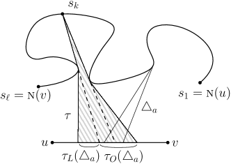
Figure 1: $\tau$ is the list of the three apexed triangles with definer $s_{k}$ sorted along $uv$. $\triangle_{a}$ overlaps with the two right apexed triangles of $\tau$ while it does not overlap with the leftmost one. $\tau_{R}(\triangle_{a})$ is empty.

3.2.1 Upper Envelopes and $\mathsf{rFVD}$

Consider any $t$ functions $f_{1},\ldots,f_{t}$ with $f_{j}:D\rightarrow\mathbb{R}\cup\{-\infty\}$ for $1\leq j\leq t$, where $D$ is a subset of $\mathbb{R}^{2}$. We define the upper envelope of $f_{i}$’s as the piecewise maximum of $f_{i}$’s. Moreover, we say that a function $f_{j}$ appears on the upper envelope if $f_{j}(x)\geq f_{i}(x)$ and $f_{j}(x)\in\mathbb{R}$ at some point $x\in D$ for any other functions $f_{i}$.

Each apexed triangle $\triangle\in A$ has a distance function $g_{\triangle}$ such that $g_{\triangle}(x)=-\infty$ for a point $x\notin\triangle$ and $g_{\triangle}(x)=d(\textsc{d}(\triangle),x)$ for a point $x\in\triangle$. In this subsection, we restrict the domain of the distance functions to $uv$. By definition, the upper envelope of $g_{\triangle}$ for all apexed triangles $\triangle\in A$ on $uv$ coincides with $\mathsf{rFVD}\cap uv$ in its projection on $uv$. We consider the sites one by one from $s_{1}$ to $s_{\ell}$ in order and compute the upper envelope of $g_{\triangle}$ for all apexed triangles $\triangle\in A$ on $uv$.

While the upper envelope of $g_{\triangle}$ for all apexed triangles $\triangle\in A$ is continuous, the upper envelope of $g_{\triangle^{\prime}}$ of all apexed triangles $\triangle^{\prime}$ with definers from $s_{1}$ up to $s_{k}$ (we simply say the upper envelope for sites from $s_{1}$ to $s_{k}$) might be discontinuous at some point on $uv$ for $1\leq k<\ell$. We let $U(s_{k})$ be the leftmost connected component of the upper envelope for sites from $s_{1}$ to $s_{k}$ along $uv$. By definition, $U(s_{\ell})=U(\textsc{n}(v))$ is the upper envelope of the distance functions of all apexed triangles in $A$. Note that $\mathsf{rCell}(\triangle)\cap uv=\emptyset$ for some apexed triangle $\triangle\in A$. Thus the distance function of some apexed triangle might not appear on $U(s_{k})$. Let $\tau_{U}(s_{k})$ be the list of the apexed triangles sorted in the order of their distance functions appearing on $U(s_{k})$. If $\textsc{d}(\triangle_{i})\neq\textsc{d}(\triangle_{i+1})$ for any two consecutive apexed triangles $\triangle_{i}$ and $\triangle_{i+1}$ of $\tau_{U}(s_{k})$, the bisector of $\textsc{d}(\triangle_{i})$ and $\textsc{d}(\triangle_{i+1})$ crosses the intersection of the bottom sides of $\triangle_{i}$ and $\triangle_{i+1}$.

3.2.2 Computing the Upper Envelope $U(s_{\ell})$

Suppose that we have $U(s_{k-1})$ and $\tau_{U}(s_{k-1})$ for some index $2\leq k\leq\ell$. We compute $U(s_{k})$ and $\tau_{U}(s_{k})$ from $U(s_{k-1})$ and $\tau_{U}(s_{k-1})$ as follows. We use two auxiliary lists $U^{\prime}$ and $\tau_{U}^{\prime}$ which are initially set to $U(s_{k-1})$ and $\tau_{U}(s_{k-1})$. We update $U^{\prime}$ and $\tau_{U}^{\prime}$ until they finally become $U(s_{k})$ and $\tau_{U}(s_{k})$, respectively. For simplicity, we use $U=U(s_{k})$, $\tau_{U}=\tau_{U}(s_{k})$ and $s=s_{k}$.

Let $\tau$ be the list of the apexed triangles of $A$ with definer $s$ sorted along $\partial P$ with respect to their bottom sides. For any apexed triangle $\triangle$, we denote the list of the apexed triangles in $\tau$ overlapping with $\triangle$ in their bottom sides by $\tau_{O}(\triangle)$. Also, we denote the lists of the apexed triangles in $\tau\setminus\tau_{O}(\triangle)$ lying left to $\triangle$ and lying right to $\triangle$ along $uv$ with respect to their bottom sides by $\tau_{L}(\triangle)$ and $\tau_{R}(\triangle)$, respectively. See Figure 1.

Let $\triangle_{a}$ denote the the rightmost apexed triangle of $\tau_{U}^{\prime}$ along $uv$. With respect to $\triangle_{a}$, we partition $\tau$ into three disjoint sublists $\tau_{L}(\triangle_{a})$, $\tau_{O}(\triangle_{a})$ and $\tau_{R}(\triangle_{a})$. We can compute these sublists in $O(|\tau|)$ time.

Case 1 : Some apexed triangles in $\tau$ overlap with $\triangle_{a}$ (i.e. $\tau_{O}(\triangle_{a})\neq\emptyset$).

Let $\triangle$ be the leftmost apexed triangle in $\tau_{O}(\triangle_{a})$ along $uv$. We compare the distance functions $g_{\triangle}$ and $g_{\triangle_{a}}$ on $\triangle_{a}\cap\triangle\cap uv$. That is, we compare $d(x,s)$ and $d(x,\textsc{d}(\triangle_{a}))$ for $x\in\triangle_{a}\cap\triangle\cap uv$.

(1) If there is a point on $\triangle_{a}\cap\triangle\cap uv$ that is equidistant from $s$ and $\textsc{d}(\triangle_{a})$, then $g_{\triangle}$ appears on $U$. Moreover, the distance functions of the apexed triangles in $\tau_{O}(\triangle_{a})\cup\tau_{R}(\triangle_{a})$ also appear on $U$, but no distance function of the apexed triangles in $\tau_{L}(\triangle_{a})$ appears on $U$ by Lemma 1. Thus we append the triangles in $\tau_{O}(\triangle_{a})\cup\tau_{R}(\triangle_{a})$. We also update $U^{\prime}$ accordingly. Then, $\tau_{U}^{\prime}$ and $U^{\prime}$ are $\tau_{U}$ and $U$, respectively.

(2) If $d(x,\textsc{d}(\triangle_{a}))>d(x,s)$ for all points $x\in\triangle_{a}\cap\triangle\cap uv$, then $\triangle$ and its distance function do not appear on $\tau_{U}$ and $U$, respectively, by Lemma 1. Thus we do nothing and scan the apexed triangles in $\tau_{O}(\triangle_{a})\cup\tau_{R}(\triangle_{a})$, except $\triangle$, from left to right along $uv$ until we find an apexed triangle $\triangle^{\prime}$ such that there is a point on $\triangle_{a}\cap\triangle^{\prime}\cap uv$ which is equidistant from $\textsc{d}(\triangle_{a})$ and $s$. Then we apply the procedure in (1) with $\triangle^{\prime}$ instead of $\triangle$. If there is no such apexed triangle, then $\tau_{U}^{\prime}$ and $U^{\prime}$ are $\tau_{U}$ and $U$, respectively.

(3) Otherwise, we have $d(x,s)>d(x,\textsc{d}(\triangle_{a}))$ for all points $x\in\triangle_{a}\cap\triangle\cap uv$. Then the distance function of $\triangle_{a}$ does not appear on $U$. Thus, we remove $\triangle_{a}$ and its distance function from $\tau_{U}^{\prime}$ and $U^{\prime}$, respectively. We consider the apexed triangles in $\tau_{L}(\triangle_{a})$ from right to left along $uv$. For an apexed triangle $\triangle^{\prime}\in\tau_{L}(\triangle_{a})$, we do the following. Since $\tau_{U}^{\prime}$ is updated, we update $\triangle_{a}$ to the rightmost element of $\tau_{U}^{\prime}$ along $uv$. We check whether $d(x,s)\geq d(x,\textsc{d}(\triangle_{a}))$ for all points $x\in\triangle_{a}\cap\triangle^{\prime}\cap uv$ if $\triangle^{\prime}$ overlaps with $\triangle_{a}$. If so, we remove $\triangle_{a}$ from $\tau_{U}^{\prime}$ and update $\triangle_{a}$ again. We do this until we find an apexed triangle $\triangle^{\prime}\in\tau_{L}(\triangle_{a})$ such that this test fails. Then, there is a point on $\triangle^{\prime}\cap\triangle_{a}\cap uv$ which is equidistant from $\textsc{d}(\triangle_{a})$ and $s$. After we reach such an apexed triangle $\triangle^{\prime}$, we apply the procedure in (1) with $\triangle^{\prime}$ instead of $\triangle$.

Case 2 : No apexed triangle in $\tau$ overlaps with $\triangle_{a}$ (i.e. $\tau_{O}(\triangle_{a})=\emptyset$).

We cannot compare the distance function of any apexed triangle in $\tau$ with the distance function of $\triangle_{a}$ directly, so we need a different method to handle this. There are two possible subcases: either $\tau_{L}(\triangle_{a})=\emptyset$ or $\tau_{R}(\triangle_{a})=\emptyset$. Note that these are the only possible subcases since the union of the apexed triangles with the same definer is connected. For the former subcase, the upper envelope of sites from $s_{1}$ to $s$ is discontinuous at the right endpoint of the bottom side of $\triangle_{a}$ along $uv$. Thus $g_{\triangle}$ does not appear on $U$ for any apexed triangle $\triangle\in\tau$. Thus $\tau_{U}^{\prime}$ and $U^{\prime}$ are $\tau_{U}$ and $U$, respectively. For the latter subcase, at most one of $s$ and $\textsc{d}(\triangle_{a})$ has a Voronoi cell in $\mathsf{FVD}[S]$ by Lemma 1. We can find a site ($s$ or $\textsc{d}(\triangle_{a})$) which does not have a Voronoi cell in $\mathsf{FVD}[S]$ in constant time once we maintain some geodesic paths. We describe this procedure at the end of this subsection.

If $s$ does not have a Voronoi cell in $\mathsf{FVD}[S]$, then $\tau_{U}^{\prime}$ and $U^{\prime}$ are $\tau_{U}$ and $U$, respectively. If $\textsc{d}(\triangle_{a})$ does not have a Voronoi cell in $\mathsf{FVD}[S]$, we remove all apexed triangles with definer $\textsc{d}(\triangle_{a})$ from $\tau_{U}^{\prime}$ and their distance functions from $U^{\prime}$. Since such apexed triangles lie at the end of $\tau_{U}^{\prime}$ consecutively, this removal process takes the time linear in the number of the apexed triangles. We repeat this until the rightmost element of $\tau$ and the rightmost element of $\tau_{U}^{\prime}$ overlap in their bottom sides along $uv$. When the two elements overlap, we apply the procedure of Case 1.

In total, the running time for computing $U(s_{\ell})$ is $O(|A|)$ since each apexed triangle in $A$ is removed from $\tau_{U}^{\prime}$ at most once. Thus, we can compute $\mathsf{rFVD}\cap\partial P$ is $O(n)$ time in total.

Maintaining Geodesic Paths for Subcase of Case 2 : $\tau_{O}(\triangle_{a})=\emptyset$ and $\tau_{R}(\triangle_{a})=\emptyset$.

We maintain $\pi(s,x)$ and its geodesic distance during the whole procedure (for all cases), where $s$ is the site we consider and $x$ is the projection of the rightmost breakpoint of $U^{\prime}$ onto $uv$. That is, $x$ is the projection of the common endpoint of the two rightmost pieces of $U^{\prime}$ onto $uv$. Recall that $s$ changes from $s_{1}$ to $s_{\ell}$. By definition, $x$ lies in the bottom side of the rightmost apexed triangle $\triangle_{a}$ of $\tau_{U}^{\prime}$. Thus we can evaluate $d(\textsc{d}(\triangle_{a}),x)$ in constant time. Note that the two points $s,x$ and the apexed triangle $\triangle_{a}$ change during the procedure. Whenever they change, we update $\pi(s,x)$ and its geodesic distance using the previous geodesic path. One of $s$ and $\textsc{d}(\triangle_{a})$ does not have a Voronoi cell in $\mathsf{FVD}[S]$ in this subcase. But it is possible that neither $s$ nor $\textsc{d}(\triangle_{a})$ has a Voronoi cell in $\mathsf{FVD}[S]$. We can decide which site does not have a Voronoi cell in $\mathsf{FVD}[S]$ in constant time: if $d(\textsc{d}(\triangle_{a}),x)>d(s,x)$, then $s$ does not have a Voronoi cell. Otherwise, $\textsc{d}(\triangle_{a})$ does not have a Voronoi cell.

We will show that the update of the geodesic path takes $O(n)$ time in total for all transition edges. Let $H_{uv}$ denote the region bounded by $uv$, $\pi(v,\textsc{n}(u))$, $\partial P[\textsc{n}(v),\textsc{n}(u)]$ and $\pi(\textsc{n}(v),u)$. The sum of the complexities $|H_{e}|$ of $H_{e}$ for all transition edges $e$ is $O(n)$ and they can be computed in $O(n)$ time (Corollary 3.8 [2]). Moreover, $|A|$ is $O(|H_{uv}|)$ (Lemma 5.2 [2]). The total complexity of the shortest path trees rooted at $u$ and $v$ in $H_{uv}$ is $O(|H_{uv}|)$, and therefore we can compute them in $O(|H_{uv}|)$ time [7]. We compute them only one for each transition edge during the whole procedure.

The edges in $\pi(s,x)$, except the edge adjacent to $x$, are also edges of the shortest path trees, and thus we can update them by traversing the shortest path trees in time linear in the amount of the changes on $\pi(s,x)$. Therefore, the following lemma implies that maintaining $\pi(s,x)$ and its length takes $O(|H_{uv}|)$ time for each transition edge $uv$.

Lemma 8.

The amount of the changes on $\pi(s,x)$ is $O(|H_{uv}|)$ during the whole procedure for $uv$.

Proof.

We claim that each edge of the shortest path trees is removed from $\pi(s,x)$ at most $O(1)$ times during the whole procedure for $uv$. Assume that we already have $\pi(s,x)$ and we are to compute $\pi(s^{\prime},x^{\prime})$. There are three different cases: (1) $x^{\prime}$ lies to the left of $x$ ($\triangle_{a}$ is removed) along $uv$, (2) $x^{\prime}$ lies to the right of $x$ (a new apexed triangle is inserted to $\tau_{U}^{\prime}$) along $uv$, and (3) we consider a new site (that is, $s^{\prime}=s_{k+1}$ and $x^{\prime}=x$.)

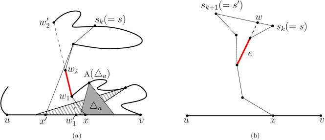
Figure 2: (a) When $\triangle_{a}$ is removed from $\tau_{U}^{\prime}$, we remove three edges from $\pi(s,x)$ to obtain $\pi(s,x^{\prime})$. (b) The edge $e$ appears on $\pi(s,x)$ for some $x\in uv$ only if $s\in\partial P[w,v]$.

For the first and the second cases, it is possible that we remove more than one edge from $\pi(s,x)$. We prove the claim for the first case only. The claim for the second case can be proved analogously. See Figure 2(a). Let $w_{1}w_{2}$ be an edge in $\pi(s,x)$ which is not adjacent to $x$ and is not in $\pi(s,x^{\prime})$ with $d(w_{1},x)<d(w_{2},x)$. Let $w_{1}^{\prime}$ and $w_{2}^{\prime}$ be the points on $\partial P$ hit by the rays from $w_{1}w_{2}$ towards $w_{1}$ and towards $w_{2}$, respectively. The right endpoint of the bottom side of $\triangle_{a}$ lies to the right of $w_{1}^{\prime}$ since $\pi(s,x)$ contains $w_{1}w_{2}$. Moreover, $s$ lies in $\partial P[w_{2}^{\prime},w_{2}]$. Thus, $\textsc{a}(\triangle_{a})$ lies in $\partial P[w_{1},v]$.

There are two possible subcases: $\textsc{d}(\triangle_{a})$ is in $\partial P[w_{2}^{\prime},w_{2}]$, or in $\partial P[w_{1},v]$. There is at most one site $s^{\prime}$ in $\partial P[w_{2}^{\prime},w_{2}]$ such that an apexed triangle with definer $s^{\prime}$ has its apex in $\partial P[w_{1},v]$ by the construction of the set of apexed triangles in [2]. (In this case, the apex lies in $\pi(w_{1},v)$.) When $w_{1}w_{2}$ is deleted, all such apexed triangles are also deleted from $\tau_{U}^{\prime}$. After $w_{1}w_{2}$ is deleted, no apexed triangle with definer in $\partial P[w_{2}^{\prime},w_{2}]$ and with apex in $\partial P[w_{1},v]$ is inserted to $\tau_{u}^{\prime}$ again. Therefore, the number of deletions of $w_{1}w_{2}$ due to the first subcase is only one. For the second subcase, notice that once $\triangle_{a}$ is removed from $\tau_{U}^{\prime}$, no apexed triangle with definer in $\partial P[w_{1},v]$ is added to $\tau_{U}^{\prime}$ again. Thus, the number of deletions of $w_{1}w_{2}$ due to the second subcase is also one.

For the third case, $s^{\prime}=s_{k+1}$ lies after $s$ from $s_{1}$ in counterclockwise order along $\partial P$. It occurs when we finish the procedure for handling $s$. After we consider the site $s^{\prime}$, we do not consider any site from $s_{1}$ to $s$ again. Consider an edge $e$ removed from $\pi(s,x)$ due to this case. Let $w$ be the point on $ss^{\prime}$ hit by the extension of $e$. See Figure 2(b). If $\pi(s,x)$ contains $e$ for some $s\in\partial P[\textsc{n}(v),\textsc{n}(u)]$ and some $x\in uv$, we have $s\in\partial P[w,v]$. This means that once $e$ is removed due to the last case, $e$ does not appear on the geodesic path $\pi(s,x)$ again in the remaining procedure. Thus, the number of deletions of each edge due to the last case is also one. ∎

Therefore, we can complete the first step in $O(n)$ time and we have the following theorem.

Theorem 9.

The geodesic farthest-point Voronoi diagram of the vertices of a simple $n$-gon $P$ restricted to the boundary of $P$ can be computed in $O(n)$ time.

4 Decomposing the Polygon into Smaller Cells

Now we have $\mathsf{rFVD}\cap\partial P$ of size $O(n)$. We add the points in $\mathsf{rFVD}\cap\partial P$ (degree-$1$ vertices of $\mathsf{rFVD}$) to the vertex set of $P$, and apply the algorithm to compute the apexed triangles with respect to the vertex set of $P$ again [2]. There is no transition edge because no additional vertex has a Voronoi cell and every degree-1 Voronoi vertex is a vertex of $P$. Thus the bottom sides of all apexed triangles are interior disjoint. Moreover, we have the set $\mathcal{A}$ of the apexed triangles sorted along $\partial P$ with respect to their bottom sides.

Definition 10.

A simple polygon $P^{\prime}\subseteq P$ is called a $t$-path-cell for some $t\in\mathbb{N}$ if it is geodesically convex and all its vertices are on $\partial P$ among which at most $t$ are convex.

In this section, we subdivide $P$ into $t$-path-cells recursively for some $t\in\mathbb{N}$ until each cell becomes a base cell. There are three types of base cells. The first type is a quadrilateral crossed by exactly one arc of $\mathsf{rFVD}$ through two opposite sides, which we call an arc-quadrilateral. The second type is a $3$-path-cell. Note that a $3$-path-cell is a pseudo-triangle. The third type is a region of $P$ whose boundary consists of one convex chain and one geodesic path (concave curve), which we call a lune-cell. Note that a convex polygon is a lune-cell whose concave chain is just a vertex of the polygon.

Let $\{t_{k}\}$ be the sequence such that $t_{1}=n$ and $t_{k}=\lfloor\sqrt{t_{k-1}}\rfloor+1$. Initially, $P$ itself is a $t_{1}$-path-cell. Assume that the $k$th iteration is completed. We show how to subdivide each $t_{k}$-path-cell with $t_{k}>3$ into $t_{k+1}$-path-cells and base cells in the $(k+1)$th iteration in Section 4.1. A base cell is not subdivided further. While subdividing a cell into a number of smaller cells recursively, we compute the refined geodesic farthest-point Voronoi diagram restricted to the boundary of each smaller cell $C$ (of any kind) in $O(|C|+|\mathsf{rFVD}\cap\partial C|)$ time. In Section 5, we show how to compute the refined geodesic farthest-point Voronoi diagram restricted to a base cell $T$ in $O(|T|+|\mathsf{rFVD}\cap\partial T|)$ time once we have $\mathsf{rFVD}\cap\partial T$. Once we compute $\mathsf{rFVD}$ restricted to every base cell, we obtain $\mathsf{rFVD}$.

4.1 Subdividing a $t$-path-cell into Smaller Cells

In this subsection, we are to subdivide each $t_{k}$-path-cell into $t_{k+1}$-path-cells and base cells. If a $t_{k}$-path-cell is a lune-cell or $t_{k}$ is at most three, the cell is a already base cell and we do not subdivide it further. Otherwise, we subdivide it using the algorithm described in this subsection.

The subdivision consists of three phases. In Phase 1, we subdivide each $t_{k}$-path-cell into $t_{k+1}$-path-cells by a curve connecting at most $t_{k+1}$ convex vertices of the $t_{k}$-path-cell. In Phase 2, we subdivide each $t_{k+1}$-path-cell further along the arcs of $\mathsf{rFVD}$ crossing the cell if there are such arcs. In Phase 3, we subdivide the cells that are created in Phase 2 and have vertices in $\mathrm{int}(P)$ into $t_{k+1}$-path-cells and lune-cells.

4.1.1 Phase 1. Subdivision by a Curve Connecting at Most $t_{k+1}$ Vertices

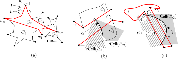
Figure 3: (a) A 16-path-cell. All convex vertices of the cell are marked with black disks. The region is subdivided into six 5-path-cells by the curve consisting of $\pi(w_{0},w_{1}),\pi(w_{1},w_{2}),\pi(w_{2},w_{3})$ and $\pi(w_{3},w_{0})$. (b) The arc $\alpha$ of $\mathsf{rFVD}$ intersects $C_{1},C_{2},C_{3}$ and crosses $C_{2}$. (c) The arc $\alpha$ of $\mathsf{rFVD}$ intersects $C_{1},C_{2},C_{3}$ and crosses $C_{2}$. Note that $\alpha$ does not cross $C_{3}$.

Let $C$ be a $t_{k}$-path-cell computed in the $k$th iteration. Recall that $C$ is a simple polygon which has at most $t_{k}$ convex vertices. Let $\beta$ be the largest integer satisfying that $\beta\lfloor\sqrt{t_{k}}\rfloor$ is less than the number of the convex vertices of $C$. Then we have $\beta\leq\lfloor\sqrt{t_{k}}\rfloor+1=t_{k+1}$.

We choose $\beta+1$ vertices $w_{0},w_{1},\ldots,w_{\beta}$ from the convex vertices of $C$ at a regular interval as follows. We choose an arbitrary convex vertex of $C$ and denote it by $w_{0}$. Then we choose the $j\lfloor\sqrt{t_{k}}\rfloor$th convex vertex of $C$ from $w_{0}$ in clockwise order and denote it by $w_{j}$ for all $j=1,\ldots,\beta$. We set $w_{\beta+1}=w_{0}$. Then we construct the closed curve $\gamma_{C}$ (or simply $\gamma$ when $C$ is clear from context) consisting of the geodesic paths $\pi(w_{0},w_{1}),\pi(w_{1},w_{2}),\ldots,(w_{\beta},w_{0})$. See Figure 3(a). In other words, the closed curve $\gamma_{C}$ is the boundary of the geodesic convex hull of $w_{0},\ldots,w_{\beta}$. Note that $\gamma$ does not cross itself. Moreover, $\gamma$ is contained in $C$ since $C$ is geodesically convex.

We compute $\gamma$ in time linear in the number of edges of $C$ using the algorithm in [15]. This algorithm takes $k$ source-destination pairs as input, where both sources and destinations are on the boundary of the polygon. It returns the geodesic path between the source and the destination for every input pair assuming that the $k$ shortest paths do not cross (but possibly overlap) one another. Computing the $k$ geodesic paths takes $O(N+k)$ time in total, where $N$ is the complexity of the polygon. In our case, the pairs $(w_{j},w_{j+1})$ for $j=0,\ldots,\beta$ are $\beta+1$ input source-destination pairs. Since the geodesic paths for all input pairs do not cross one another, $\gamma$ can be computed in $O(\beta+|C|)=O(|C|)$ time. Then we compute $\mathsf{rFVD}\cap\gamma$ in $O(|C|+|\mathsf{rFVD}\cap\partial C|)$ time using $\mathsf{rFVD}\cap\partial C$ obtained from the $k$th iteration. We will describe this procedure in Section 4.2.

The curve $\gamma$ subdivides $C$ into $t_{k+1}$-path-cells. To be specific, $C\setminus\gamma$ consists of at least $\beta+2$ connected components. Note that the closure of each connected component is a $t_{k+1}$-path-cell. Moreover, the union of the closures of all connected components is exactly $C$ since $C$ is simple. These components define the subdivision of $C$ induced by $\gamma$.

4.1.2 Phase 2. Subdivision along an Arc of $\mathsf{rFVD}$

After subdividing $C$ into $t_{k+1}$-path-cells $C_{1},\ldots,C_{\delta}$ $(\delta\geq\beta+2)$ by the curve $\gamma_{C}$, an arc $\alpha$ of $\mathsf{rFVD}$ may cross $C_{j}$ for some $1\leq j\leq\delta$. We say an arc $\alpha$ of $\mathsf{rFVD}$ crosses a cell $C^{\prime}$ if $\alpha$ intersects at least two distinct edges of $C^{\prime}$. For example, in Figure 3(c), $\alpha$ crosses $C_{2}$ while $\alpha$ does not cross $C_{3}$ because $\alpha$ crosses only one edge of $C_{3}$. In Phase 2, for each arc $\alpha$ crossing $C_{j}$, we isolate the subarc $\alpha\cap C_{j}$. That is, we subdivide $C_{j}$ further into three subcells so that only one of them intersects $\alpha$. We call such a subcell an arc-quadrilateral. Moreover, for an arc-quadrilateral $\square$ created by an arc $\alpha$ crossing $C_{j}$, we have $\mathsf{rFVD}\cap\square=\alpha\cap C_{j}$.

Lemma 11.

For a geodesic convex polygon $C$ with $t$ convex vertices ($t\in\mathbb{N}$), let ${\gamma}$ be a simple closed curve connecting at most $t$ convex vertices of $C$ lying on $\partial P$ such that every two consecutive vertices are connected by a geodesic path. Then, each arc $\alpha$ of $\mathsf{rFVD}$ intersecting $C$ intersects at most three cells in the subdivision of $C$ induced by ${\gamma}$ and at most two edges of $\gamma$.

Proof.

Consider an arc $\alpha$ of $\mathsf{rFVD}$ intersecting $C$. The arc $\alpha$ is a part of either a side of some apexed triangle or the bisector of two sites. For the first case, the arc $\alpha$ is a line segment. Thus $\alpha$ intersects at most three cells in the subdivision of $C$ by ${\gamma}$ and at most two edges of $\gamma$. For the second case, $\alpha$ is part of a hyperbola. Let $s_{1}$ and $s_{2}$ be the two sites defining $\alpha$ in $\mathsf{rFVD}$. The combinatorial structure of the geodesic path from $s_{1}$ (or $s_{2}$) to any point in $\alpha$ is the same. This means that $\alpha$ is contained in the intersection of two apexed triangles $\triangle_{1}$ and $\triangle_{2}$, one with definer $s_{1}$ and the other with definer $s_{2}$. Observe that $\triangle_{1}\cap\triangle_{2}$ intersects ${\gamma}$ at most twice and contains no vertex of ${\gamma}$ in its interior. By construction, $\triangle_{1}\cap\triangle_{2}$ intersects at most two edges $e_{1}$ and $e_{2}$ of ${\gamma}$, and thus so does $\alpha$. For a cell $C^{\prime}$ in the subdivision of $C$ by ${\gamma}$, the arc $\alpha$ intersects $C^{\prime}$ if and only if $C^{\prime}$ contains $e_{1}$ or $e_{2}$ on its boundary. Thus there exist at most three such cells in the subdivision of $C$ by ${\gamma}$ and the lemma holds for the second case. See Figure 3(b-c). ∎

First, we find $\alpha\cap C_{j}$ for every arc $\alpha$ of $\mathsf{rFVD}$ crossing $C_{j}$. If $\mathsf{rCell}(\triangle)\cap\partial C_{j}$ consists of at most two connected components (line segments) for every apexed triangle $\triangle\in\mathcal{A}$, we can do this by scanning all points in $\mathsf{rFVD}\cap\partial C_{j}$ along $\partial C_{j}$. However, $\mathsf{rCell}(\triangle)\cap\partial C_{j}$ might consist of more than two connected components (line segments) for some apexed triangle $\triangle\in\mathcal{A}$. See Figure 4. Despite of this fact, we can compute all such arcs in $O(|\mathsf{rFVD}\cap\partial C_{j}|)$ time by the following lemma.

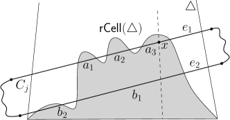
Figure 4: $\mathsf{rCell}(\triangle)\cap\partial C_{j}$ consists of five connected components $a_{i}$ contained in $e_{1}$ and $b_{j}$ contained in $e_{2}$ for $i=1,2,3$ and $j=1,2$.

Lemma 12.

For every arc $\alpha$ of $\mathsf{rFVD}$ crossing $C_{j}$, we can find the part of $\alpha$ contained in $C_{j}$ in $O(|\mathsf{rFVD}\cap\partial C_{j}|)$ time in total. Moreover, for each such arc $\alpha$, the pair $(\triangle_{1},\triangle_{2})$ of apexed triangles such that $\alpha\cap C_{j}=\{x\in C_{j}:g_{\triangle_{1}}(x)=g_{\triangle_{2}}(x)>0\}$ can be found in the same time.

Proof.

For each apexed triangle $\triangle\in\mathcal{A}$ intersecting $C_{j}$, we find all connected components of $\mathsf{rCell}(\triangle)\cap\partial C_{j}$. Since we already have $\mathsf{rFVD}\cap\partial C_{j}$, this takes $O(|\mathsf{rFVD}\cap\partial C_{j}|)$ time for all apexed triangles in $\mathcal{A}$ intersecting $C_{j}$. There are at most two edges of $\partial C_{j}$ that are intersected by $\mathsf{rCell}(\triangle)$ due to Lemma 11. Let $e_{1}$ and $e_{2}$ be such edges, and we assume that $e_{1}$ contains the point in $\mathsf{rCell}(\triangle)\cap\partial C_{j}$ closest to $\textsc{a}(\triangle)$ without loss of generality. We insert all connected components of $\mathsf{rCell}(\triangle)\cap e_{1}$ in the clockwise order along $\partial C_{j}$ into a queue. Then, we consider the connected components of $\mathsf{rCell}(\triangle)\cap e_{2}$ in the clockwise order along $\partial C_{j}$ one by one.

To handle a connected component $r$ of $\mathsf{rCell}(\triangle)\cap e_{2}$, we do the following. Let $x$ be a point in the first element $r^{\prime}$ of the queue. If the line passing through $x$ and $\textsc{a}(\triangle)$ intersects $r$, then we remove $r^{\prime}$ from the queue and check whether $r$ and $r^{\prime}$ are incident to the same refined cell $\mathsf{rCell}(\triangle^{\prime})$. If so, we compute the part of the arc defined by $\triangle$ and $\triangle^{\prime}$ inside $C_{j}$, and return the part of the arc and the pair $(\triangle,\triangle^{\prime})$. If $r$ and $r^{\prime}$ are not incident to the same refined cell, we remove $r^{\prime}$ from the queue since. We repeat this until the line passing through a point of the first element of the queue does not intersect $r$. Then we handle the connected component of $\mathsf{rCell}(\triangle)\cap e_{2}$ next to $r$.

Every arc computed from this procedure is an arc of $\mathsf{rFVD}$ crossing $C_{j}$. The remaining work is to show that we can find all arcs of $\mathsf{rFVD}$ crossing $C_{j}$ using this procedure. Consider an arc $\alpha$ of $\mathsf{rFVD}$ crossing $C_{j}$. There are two connected components $r\subseteq e_{1}$ and $r^{\prime}\subseteq e_{2}$ of $\mathsf{rFVD}(\triangle)\cap\partial C_{j}$ incident to a point in $\alpha\cap\partial C_{j}$. The line passing through any point $x\in\alpha\cap C_{j}$ and $\textsc{a}(\triangle)$ intersects $e_{2}$ once. Moreover, this intersection is in $\mathsf{rCell}(\triangle)$ by Lemma 4. Since $r^{\prime}$ contains the set of all such intersections, the line passing through a point in $r$ and $\textsc{a}(\triangle)$ intersects $r^{\prime}$. Thus the procedure finds $\alpha$. ∎

By Lemma 11, $\alpha\cap C_{j}$ consists of at most two connected components. For the case that it consists of exactly two connected components, we consider each connected component separately. In the following, we consider only the case that $\alpha\cap C_{j}$ is connected.

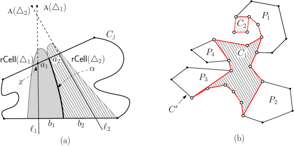
Figure 5: (a) The arc $\alpha$ of $\mathsf{rFVD}$ crosses $C_{j}$. We isolate $\alpha$ by subdividing $C_{j}$ into three subcells with respect to $\ell_{1}$ and $\ell_{2}$. (b) The vertices marked with empty disks are the vertices of $P$ while the others are vertices of arc-quadrilaterals lying in $\mathrm{int}(P)$. We subdivide the cell into two $t$-path-cells $C_{1},C_{2}$ and four lune-cells $P_{1},\ldots,P_{4}$.

For an arc $\alpha$ crossing $C_{j}$, we subdivide $C_{j}$ further into two cells with $t^{\prime}$ convex vertices for $t^{\prime}\leq t_{k+1}$ and one arc-quadrilateral by adding two line segments bounding $\alpha$ so that no arc other than $\alpha$ intersects the arc-quadrilateral. Let $(\triangle_{1},\triangle_{2})$ be the pair of apexed triangles defining $\alpha$. Let $a_{1},b_{1}$ (and $a_{2},b_{2}$) be the two connected components of $\mathsf{rCell}(\triangle_{1})\cap\partial C_{j}$ (and $\mathsf{rCell}(\triangle_{2})\cap\partial C_{j}$) incident to $\alpha$ such that $a_{1},a_{2}$ are adjacent to each other and $b_{1},b_{2}$ are adjacent to each other. See Figure 5(a). Without loss of generality, we assume that $a_{1}$ is closer than $b_{1}$ to $\textsc{a}(\triangle_{1})$. Let $x$ be any point on $a_{1}$. Then the $V$-farthest neighbor of $x$ is the definer of $\triangle_{1}$. We consider the line $\ell_{1}$ passing through $x$ and the apex of $\triangle_{1}$. Then the intersection between $C_{j}$ and $\ell_{1}$ is contained in the closure of $\mathsf{rCell}(\triangle_{1})$ by Lemma 4. Similarly, we find the line $\ell_{2}$ passing through the apex of $\triangle_{2}$ and a point on $a_{2}$.

We subdivide $C_{j}$ into two cells with at most $t_{k+1}$ convex vertices and one arc-quadrilateral by $\ell_{1}$ and $\ell_{2}$. The quadrilateral bounded by the two lines and $\partial C_{j}$ is an arc-quadrilateral since $\alpha$ crosses the quadrilateral but no other arcs of $\mathsf{rFVD}$ intersect the quadrilateral. We do this for all arcs crossing $C_{j}$. Note that no arc crosses the resulting cells other than arc-quadrilaterals by the construction. The resulting cells with at most $t_{k+1}$ convex vertices and arc-quadrilaterals are the cells in the subdivision of $C$ obtained from Phase 2. Therefore, we have the following lemma.

Lemma 13.

No arc of $\mathsf{rFVD}$ crosses cells other than arc-quadrilaterals created in Phase 2.

4.1.3 Phase 3. Subdivision by a Geodesic Convex Hull

Note that some cell $C^{\prime}$ with $t^{\prime}$ convex vertices for $3<t^{\prime}\leq t_{k+1}$ created in Phase 2 might be neither a $t^{\prime}$-path-cell nor a base cell. This is because a cell created in Phase 2 might have some vertices in $\mathrm{int}(P)$. In Phase 3, we subdivide such cells further into $t^{\prime}$-path-cells and lune-cells.

To subdivide $C^{\prime}$ into $t_{k+1}$-path-cells and lune-cells, we first compute the geodesic convex hull $\mathsf{CH}$ of the vertices of $C^{\prime}$ which come from the vertex set of $P$ in time linear in the number of edges in $C^{\prime}$ using the algorithm for computing $k$ shortest paths in [15]. Consider the connected components of $C^{\prime}\setminus\partial\mathsf{CH}$. They belong to one of two types defined as follows. A connected component of the first type is enclosed by a closed simple curve which is part of $\partial\mathsf{CH}$. For example, $C_{1}$ and $C_{2}$ in Figure 5(b) are the connected components belonging to this type. A connected component of the second type is enclosed by a subchain of $\partial\mathsf{CH}$ from $u$ to $w$ in clockwise order and a subchain of $\partial C^{\prime}$ from $w$ to $u$ in counterclockwise order for some $u,w\in\partial P$. For example, $P_{i}$ in Figure 5(b) is the connected component belonging to the second type for $i=1,\ldots,4$.

By the construction, a connected component belonging to the first type has all its vertices from the vertex set of $P$. Moreover, it has at most $t^{\prime}$ convex vertices since $C^{\prime}$ has $t^{\prime}$ convex vertices. Therefore, the closure of a connected component of $C^{\prime}\setminus\partial\mathsf{CH}$ belonging to the first type is a $t^{\prime}$-path-cell with $t^{\prime}\leq t_{k+1}$.

Every vertex of $C^{\prime}$ lying in $\mathrm{int}(P)$ is convex with respect to $C^{\prime}$ by the construction of $C^{\prime}$. Thus, for a connected component $P^{\prime}$ belonging to the second type, the part of $\partial P^{\prime}$ from $\partial C^{\prime}$ is a convex chain with respect to $P^{\prime}$. Moreover, the part of $\partial P^{\prime}$ from $\partial\mathsf{CH}$ is the geodesic path between two points, and thus it is a concave chain with respect to $P^{\prime}$. Therefore, the closure of a connected component belonging to the second type is a lune-cell.

Since $C^{\prime}$ is a simple polygon, the union of the closures of all connected components of $C^{\prime}\setminus\mathsf{CH}$ is exactly the closure of $C^{\prime}$. The closures of all connected components belonging to the first and the second types are $t_{k+1}$-path-cells and lune-cells created at the end of the $(k+1)$th iteration, respectively. We compute the $t_{k+1}$-path-cells and the lune-cells induced by $\partial\mathsf{CH}$. Then, we compute $\mathsf{rFVD}\cap\partial\mathsf{CH}$ using the procedure in Section 4.2.

The resulting $t_{k+1}$-path-cells and base cells form the final decomposition of $C$ of the $(k+1)$th iteration.

4.1.4 Analysis of the Complexity

We first give the combinatorial complexity of the refined geodesic farthest-point Voronoi diagram restricted to the boundary of the cells from each iteration. Note that an arc of $\mathsf{rFVD}$ might cross some $t_{k}$-path-cells in the decomposition at the end of the $k$th iteration for any $k$ while no arc of $\mathsf{rFVD}$ crosses cells other than arc-quadrilaterals created in Phase 2. The following lemma is used to prove the complexity.

Lemma 14.

An arc $\alpha$ of $\mathsf{rFVD}$ intersects at most nine $t_{k}$-path-cells and $O(k)$ base cells at the end of the $k$th iteration for any $k\in\mathbb{N}$. Moreover, there are at most three $t_{k}$-path-cells that $\alpha$ intersects but does not cross at the end of the $k$th iteration.

Proof.

Let $\alpha$ be an arc of $\mathsf{rFVD}$. If $\alpha$ is a line segment, the lemma holds directly. Thus, we consider the case that $\alpha$ is a part of hyperbola defined by a pair $(\triangle_{1},\triangle_{2})$ of apexed triangles. That is, $\alpha\subseteq\{x\in\triangle_{1}\cap\triangle_{2}:g_{\triangle_{1}}(x)=g_{\triangle_{2}}(x)\geq 0\}$.

We first show that there is at most one $t_{k}$-path-cell at the end of the $k$th iteration that $\alpha$ intersects but does not cross, and no endpoint of $\alpha$ is contained in. Assume to the contrary that there are two such $t_{k}$-path-cells. Consider two edges $e_{1}$ and $e_{2}$ from the two cells which intersect $\alpha$. Notice that they are distinct.

We claim that $e_{1}$ and $e_{2}$ intersect at some point other than their endpoints, which makes a contradiction. To prove the claim, we assume that the line containing $\textsc{a}(\triangle_{1})$ and $\textsc{a}(\triangle_{2})$ is the $x$-axis. Then $\alpha$ is part of a hyperbola whose foci lie on the $x$-axis. The arc $\alpha$ does not intersect the $x$-axis. Let $h_{1}$ and $h_{2}$ be the lines tangent to the hyperbola containing $\alpha$ at the endpoints of $\alpha$. We denote the region bounded by $h_{1}$, $h_{2}$ and $\alpha$ by $R$. Then to prove the claim, it suffices to show that $R$ is contained in $\triangle_{1}\cap\triangle_{2}$ because no vertex lies in the interior of $\triangle_{1}\cap\triangle_{2}$. Assume that $R$ is not contained in $\triangle_{1}$. Then one of the sides of $\triangle_{1}$ incident to $\textsc{a}(\triangle_{1})$ intersects $R$. Thus, there is a line passing through $\textsc{a}(\triangle_{1})$ which intersects $\alpha$ twice by the property of the hyperbola, which is a contradiction by Lemma 4. The case that $R$ is not contained in $\triangle_{2}$ is analogous. Therefore, the claim holds. Including the two $t_{k}$-path-cells containing an endpoint of $\alpha$, there are at most three $t_{k}$-path-cells that $\alpha$ intersects but does not cross.

Now we show that $\alpha$ intersects at most nine $t_{k}$-path-cells and $O(k)$ base cells at the end of the $k$th iteration. For $k=1$, $P$ itself is the decomposition of $P$, thus there exists only one cell. For $k\geq 2$, assume that the lemma holds for the $k^{\prime}$th iterations for all $k^{\prime}<k$.

We claim that the $k$th iteration creates a constant number of the arc-quadrilaterals that $\alpha$ intersect. Due to the assumption, $\alpha$ intersects at most nine $t_{k-1}$-path-cells at the end of the $(k-1)$th iteration. Thus, at the end of Phase 1 of the $k$th iteration, $\alpha$ crosses at most 27 $t_{k}$-path-cells by Lemma 11. Note that $\alpha\cap C^{\prime}$ might consist of two connected components for a $t_{k}$-path-cell $C^{\prime}$ created in Phase 1. See Figure 3(c). In this case, we create two arc-quadrilaterals. If $\alpha\cap C^{\prime}$ is connected, we create one arc-quadrilateral. Thus, we create at most 54 arc-quadrilaterals crossed by $\alpha$ in the $k$th iteration. Therefore, in the $k$th iteration, there are $O(k)$ arc-quadrilaterals intersecting $\alpha$.

We claim that the number of the $t_{k}$-path-cells that $\alpha$ intersects at the end of the $k$th iteration is at most nine. There are three cells from Phase 2 other than arc-quadrilaterals intersecting $\alpha$. Note that $\alpha$ does not cross more than two cells. Thus, it is sufficient to consider only these three cells. Each cell $C$ from Phase 2 intersecting $\alpha$ is subdivided into smaller cells in Phase 3. Due to Lemma 11, at most three smaller cells intersect $\alpha$. Thus, in total, the $k$th iteration creates at most nine cells of the $t_{k}$-path-cells that $\alpha$ intersects. Similarly, we can prove that the $k$th iteration creates a constant number of lune-cells intersecting $\alpha$. Therefore, the lemma holds. ∎

Now we are ready to prove the complexities of the cells and $\mathsf{rFVD}$ restricted to the cells in each iteration. Then we finally prove that the running time of the algorithm in this section is $O(n\log\log n)$.

Lemma 15.

At the end of the $k$th iteration for any $k\in\mathbb{N}$, the following holds.

• $\sum_{C:\textnormal{a }t_{k}\textnormal{-path-cell}}{|\mathsf{rFVD}\cap\partial C|}=O(n)$.

• $\sum_{C:\textnormal{a }t_{k}\textnormal{-path-cell}}{|C|}=O(n)$.

• $\sum_{T:\textnormal{a base cell}}{|\mathsf{rFVD}\cap\partial T|}=O(kn)$.

• $\sum_{T:\textnormal{a base cell}}{|T|}=O(kn)$.

Proof.

Let $\alpha$ be an arc of $\mathsf{rFVD}$. The first and the third complexity bounds hold by Lemma 14 and the fact that the number of the arcs of $\mathsf{rFVD}$ is $O(n)$.

The second complexity bound holds since the set of all edges of the $t_{k}$-path-cells is a subset of the chords in some triangulation of $P$. Any triangulation of $P$ has $O(n)$ chords. Moreover, each chord is incident to at most two $t_{k}$-path-cells.

For the last complexity bound, the number of the edges of the base cells whose endpoints are vertices of $P$ is $O(n)$ since they are chords in some triangulation of $P$. Thus we count the number of edges of the base cells which are not incident to vertices of $P$. In Phase 1, we do not create any such edge. In Phase 2, we create at most $O(1)$ such edges whenever we create one arc-quadrilateral. All edges created in Phase 3 have their endpoints from the vertex set of $P$. Therefore, the total number of the edges of all base cells is asymptotically bounded by the number of arc-quadrilaterals, which is $O(kn)$. ∎

Corollary 16.

In $O(\log\log n)$ iterations, the polygon is subdivided into $O(n\log\log n)$ base cells.

Lemma 17.

The subdivision in each iteration can be done in $O(n)$ time.

Proof.

In Phase 1, we compute $\gamma$ and $\mathsf{rFVD}\cap\gamma$ for each $t$-path-cell $C$ from the previous iteration. The running time for this is linear in the total complexity of all $t$-path-cells in the previous iteration and $\mathsf{rFVD}$ restricted on the boundary of all $t$-path-cells by Lemma 20, which is $O(n)$ by Lemma 15.

In Phase 2, we first scan $\mathsf{rFVD}\cap\partial C^{\prime}$ for all cells $C^{\prime}$ from Phase 1 to find an arc of $\mathsf{rFVD}$ crossing some cell. This can also be done in linear time by Lemma 12 and Lemma 15. For each arc crossing some $t$-path-cell, we compute two line segments bounding the arc and subdivide the cell into two smaller regions and one arc-quadrilateral in $O(1)$ time. Each arc of $\mathsf{rFVD}$ crosses at most $O(1)$ cells from Phase 1, and the time for this step is $O(n)$ in total.

In Phase 3, we further subdivide each cell which is not a base cell from Phase 2. In the subdivision of a cell which is not a base cell $C$ in Phase 2, we first compute the geodesic convex hull $\mathsf{CH}$ of the vertices of $C^{\prime}$ which are vertices of $P$. The geodesic convex hull can be computed in time linear in the complexity of $C^{\prime}$. By Lemma 20, $\mathsf{rFVD}\cap\partial\mathsf{CH}$ can be computed in $O(|\mathsf{rFVD}\cap\partial C^{\prime}|+|C^{\prime}|)$ time. Note that all cells other than the base cells from Phase 2 are interior disjoint. Moreover, the total number of the edges of such cells is $O(n)$. Similarly, the total complexity of $\mathsf{rFVD}\cap\partial C^{\prime}$ for all such cells $C^{\prime}$ is $O(n)$. Therefore, the $t$-path-cells and lune-cells can be computed in $O(n)$ time. ∎

4.2 Computing $\mathsf{rFVD}$ Restricted to a Curve Connecting Vertices of $P$

In this section, we describe a procedure to compute $\mathsf{rFVD}\cap\gamma$ in $O(|\mathsf{rFVD}\cap\partial C|+|C|)$ time once we have $\mathsf{rFVD}\cap\partial C$, where $C\subseteq P$ is a geodesic convex polygon and $\gamma$ is a simple closed curve connecting some convex vertices of $C$ lying on $\partial P$ in clockwise order along $\partial C$ by the geodesic paths connecting two consecutive vertices. For an apexed triangle $\triangle$ with $\mathsf{rCell}(\triangle)\cap\gamma\neq\emptyset$, we have $\mathsf{rCell}(\triangle)\cap\partial C\neq\emptyset$ by Lemma 4. Thus we consider only the apexed triangles $\triangle$ with $\mathsf{rCell}(\triangle)\cap\partial C\neq\emptyset$. Let $\mathcal{L}$ be the list of all such apexed triangles sorted along $\partial P$ with respect to their bottom sides. (Recall that the bottom sides of all apexed triangles are interior-disjoint. Moreover, the union of them is $\partial P$ by the construction.) Note that $|\mathcal{L}|=O(|\mathsf{rFVD}\cap\partial C|)$.

Consider a line segment $ab$ contained in $P$. Without loss of generality, we assume that $ab$ is horizontal and $a$ lies to the left of $b$. Let $\triangle_{a}$ and $\triangle_{b}$ be the apexed triangles that maximize $g_{\triangle_{a}}(a)$ and $g_{\triangle_{b}}(b)$, respectively. If there is a tie by more than one apexed triangle, we choose an arbitrary one of them. Note that $\mathsf{rCell}(\triangle_{a})$ and $\mathsf{rCell}(\triangle_{b})$ contain $a$ and $b$ in their closures, respectively. With the two apexed triangles, we define two sorted lists $\mathcal{L}_{ab}$ and $\mathcal{L}_{ba}$ as follows. Let $\mathcal{L}_{ab}$ be the sorted list of the apexed triangles in $\mathcal{L}$ which intersect $ab\setminus\{a,b\}$ and whose bottom sides on $\partial P$ lie from the bottom side of $\triangle_{a}$ to the bottom side of $\triangle_{b}$ including $\triangle_{a}$ and $\triangle_{b}$ in clockwise order along $\partial P$. Similarly, let $\mathcal{L}_{ba}$ be the sorted list of the apexed triangles in $\mathcal{L}$ which intersect $ab\setminus\{a,b\}$ and whose bottom sides lie from the bottom side of $\triangle_{b}$ to the bottom side of $\triangle_{a}$ including $\triangle_{a}$ and $\triangle_{b}$ in clockwise order along $\partial P$. Note that no apexed triangle other than $\triangle_{a}$ and $\triangle_{b}$ appears both $\mathcal{L}_{ab}$ and $\mathcal{L}_{ba}$. See Figure 6(a).

The following lemma together with Section 4.2.1 gives a procedure to compute $\mathsf{rFVD}\cap ab$. This procedure is similar to the procedure in Section 3 that computes $\mathsf{rFVD}$ restricted to $\partial P$.

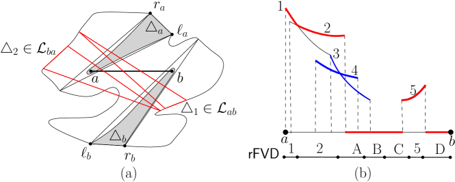
Figure 6: (a) The apexed triangles with their bottom sides in $\partial P[\ell_{a},r_{b}]$ and $\partial P[\ell_{b},r_{a}]$ are in $\mathcal{L}_{ab}$ and $\mathcal{L}_{ba}$, respectively. $\triangle_{1}\in\mathcal{L}_{ab}$ and $\triangle_{2}\in\mathcal{L}_{ba}$. (b) The hyperbolic arcs are the graphs of the distance functions associated with the apexed triangles in $\mathcal{L}_{ab}$. Curves 1, 2, and 5 represent a partial upper envelope of all distance functions. Note that curves 3 and 4 do not appear on the complete upper envelope which coincides with $\mathsf{rFVD}$ because curves A and B from $\mathcal{L}_{ba}$ appear on the complete upper envelope.

Lemma 18.

Let $C$ be a geodesic convex polygon, and let $a$ and $b$ be two points with $ab\subset C$. Given the two sorted lists $\mathcal{L}_{ab}$ and $\mathcal{L}_{ba}$, we can compute $\mathsf{rFVD}\cap ab$ in $O(|\mathcal{L}_{ab}|+|\mathcal{L}_{ba}|)$ time.

Proof.

Recall that the upper envelope of $g_{\triangle}$ on $ab$ for all apexed triangles $\triangle\in\mathcal{L}_{ab}\cup\mathcal{L}_{ba}$ (simply, the upper envelope for $\mathcal{L}_{ab}\cup\mathcal{L}_{ba}$) coincides with $\mathsf{rFVD}\cap ab$ in its projection on $ab$ by definition. Thus we compute the upper envelope for $\mathcal{L}_{ab}\cup\mathcal{L}_{ba}$. To this end, we compute a “partial” upper envelope of $g_{\triangle}$ on $ab$ for all apexed triangles $\triangle\in\mathcal{L}_{ab}$. After we do this also for the apexed triangles in $\mathcal{L}_{ba}$, we merge the two “partial” upper envelopes on $ab$ to obtain the complete upper envelope of $g_{\triangle}$ on $ab$ for all apexed triangles $\triangle\in\mathcal{L}_{ab}\cup\mathcal{L}_{ba}$.

A partial upper envelope for $\mathcal{L}_{ab}$ is the upper envelope for $A\subseteq\mathcal{L}_{ab}$ satisfying that $\triangle\in\mathcal{L}_{ab}$ belongs to $A$ if $\mathsf{rCell}(\triangle)\cap ab\neq\emptyset$. Here, an apexed triangle $\triangle\in A$ does not necessarily have a refined Voronoi cell on $ab$. Thus, a partial upper envelope for $\mathcal{L}_{ab}$ (and $\mathcal{L}_{ba}$) is not necessarily unique. The upper envelope of two partial upper envelopes, one for $\mathcal{L}_{ab}$ and one for $\mathcal{L}_{ba}$, is the complete upper envelope for $\mathcal{L}_{ab}\cup\mathcal{L}_{ba}$ by definition. See Figure 6(b).

In the following, we show how to compute one of the partial upper envelopes for $\mathcal{L}_{ab}$. A partial upper envelope for $\mathcal{L}_{ba}$ can be computed analogously. Then the complete upper envelope can be constructed in $O(|\mathcal{L}_{ab}|+|\mathcal{L}_{ba}|)$ time by scanning the two partial upper envelopes along $ab$.

For any two apexed triangles $\triangle_{1},\triangle_{2}\in\mathcal{L}_{ab}$ such that $\triangle_{1}$ comes before $\triangle_{2}$ in the sorted list $\mathcal{L}_{ab}$, $\mathsf{rCell}(\triangle_{1})\cap ab$ lies to the left of $\mathsf{rCell}(\triangle_{2})\cap ab$ along $uv$ if they exist. If it is not true, there is a point contained in $\mathsf{rCell}(\triangle_{1})\cap\mathsf{rCell}(\triangle_{2})$ by Lemma 4, which contradicts that all refined cells are pairwise disjoint. With this property, a partial upper envelope for $\mathcal{L}_{ab}$ can be constructed in a way similar to the procedure for computing $\mathsf{rFVD}\cap\partial P$ in Section 3.2. The difficulty here is that we must avoid maintaining geodesic paths as it takes $O(n)$ time, which is too much for our purpose.

We consider the apexed triangles in $\mathcal{L}_{ab}$ from $\triangle_{a}$ to $\triangle_{b}$ one by one as follows. Let $U$ be the current partial upper envelope of the distance functions of the apexed triangles from $\triangle_{a}$ to $\triangle^{\prime}$ of $\mathcal{L}_{ab}$ and $\tau$ be the list of the apexed triangles whose distance functions restricted to $ab$ appear on $U$ in the order in which they appear on $U$. Note that $U$ is not necessarily continuous. We maintain all connected components of $U$ here while we maintain only one connected component of $U$ in Section 3. We show how to update $U$ to a partial upper envelope of the distance functions of the apexed triangles from $\triangle_{a}$ to $\triangle$, where $\triangle$ is the apexed triangle next to $\triangle^{\prime}$ in $\mathcal{L}_{ab}$. Let $\triangle_{r}$ be the last element in $\tau$ and $\mu$ be the line segment contained in $ab$ such that $g_{\triangle_{r}}(x)=U(x)>0$ for every point $x\in\mu$.

There are three possibilities: (1) $\triangle\cap\mu\neq\emptyset$. In this case, we compare the distance functions of $\triangle$ and $\triangle_{r}$ on $\triangle\cap\mu$. Depending on the result, we update $U$ and $\tau$ as we did in Section 3.2. (2) $\triangle\cap\mu=\emptyset$ and $\triangle\cap ab$ lies to the right of $\mu$. We append $\triangle$ to $\tau$ at the end and update $U$ accordingly. (3) $\triangle\cap\mu=\emptyset$ and $\triangle\cap ab$ lies to the left of $\mu$. We have to use a method different from the one in Section 3.2 to handle this case. Here, contrast to the case in Section 3.2, $\triangle_{r}$ intersects $\triangle$. Thus, we can check whether $\mathsf{rCell}(\triangle)\cap ab=\emptyset$ or $\mathsf{rCell}(\triangle_{r})\cap ab=\emptyset$ easily as follows. Consider the set $R=\triangle\cap\triangle_{r}$. The distance functions associated with $\triangle$ and $\triangle_{r}$ have positive values on $R$, and thus we can compare the geodesic distances from $\textsc{d}(\triangle)$ and $\textsc{d}(\triangle_{r})$ to any point in $R$. Depending on the result, we can check in constant time whether $\mathsf{rCell}(\triangle)$ and $\mathsf{rCell}(\triangle_{r})$ intersect the connected regions $\triangle\setminus R$ and $\triangle_{r}\setminus R$ containing $\textsc{a}(\triangle)$ and $\textsc{a}(\triangle_{r})$, respectively. If $\mathsf{rCell}(\triangle)$ does not intersect the connected region $\triangle\setminus R$ containing $\textsc{a}(\triangle)$, then $\mathsf{rCell}(\triangle_{r})$ does not intersect $ab$. This also holds for $\mathsf{rCell}(\triangle_{r})$. Depending on the result, we apply the procedure in Section 3.2.

In this way, we append an apexed triangle $\triangle$ to $\tau$ if $\mathsf{rCell}(\triangle)\cap ab\neq\emptyset$. Similarly, we remove some apexed triangle $\triangle$ from $\tau$ only if $\mathsf{rCell}(\triangle)\cap ab=\emptyset$. Thus, by definition, $U$ is a partial upper envelope of the distance functions for $\mathcal{L}_{ab}$.

As mentioned above, we do this also for $\mathcal{L}_{ba}$. Then we compute the upper envelope of the two resulting partial upper envelopes, which is the complete upper envelope for $\mathcal{L}_{ab}\cup\mathcal{L}_{ba}$. This takes $O(|\mathcal{L}_{ab}|+|\mathcal{L}_{ba}|)$ time. ∎

Corollary 19.

Let $C$ be a geodesic convex polygon and $E$ be a set of $O(1)$ line segments which are contained in $C$. Then $\mathsf{rFVD}\cap ab$ for all $ab\in E$ can be computed in $O(|\mathsf{rFVD}\cap\partial C|)$ time.

Due to Lemma 18, we can compute $\mathsf{rFVD}\cap\gamma$ in $O(\sum_{ab\in\gamma}{|\mathcal{L}_{ab}|+|\mathcal{L}_{ba}|})$ time once we compute $\mathcal{L}_{ab}$ and $\mathcal{L}_{ba}$ for all edges $ab$ of $\gamma$. Recall that every apexed triangle in $\mathcal{L}_{ab}\cup\mathcal{L}_{ba}$ intersects $ab$ by the definitions of $\mathcal{L}_{ab}$ and $\mathcal{L}_{ba}$. Since every apexed triangle intersects $\gamma$ in at most two edges, each apexed triangle in $\mathcal{L}$ is contained in $\mathcal{L}_{ab}\cup\mathcal{L}_{ba}$ for at most two edges $ab$ of $\gamma$. Therefore, once we have $\mathcal{L}_{ab}$ and $\mathcal{L}_{ba}$ for every edge $ab$ of $\gamma$, we can compute $\mathsf{rFVD}\cap\gamma$ in $O(|\mathcal{L}|)=O(|\mathsf{rFVD}\cap\partial C|)$ time. The remaining procedure is computing $\mathcal{L}_{ab}$ and $\mathcal{L}_{ba}$ for all edges $ab$ of $\gamma$.

4.2.1 Computing $\mathcal{L}_{ab}$ and $\mathcal{L}_{ba}$ for All Edges $ab$ of $\gamma$

We show how to compute $\mathcal{L}_{ab}$ and $\mathcal{L}_{ba}$ for all edges $ab$ of $\gamma$ in $O(|\mathcal{L}|+|C|)$ time. By definition, every vertex of $\gamma$ is a vertex of $P$. Let $ab$ be an edge of $\gamma$, where $b$ is the clockwise neighbor of $a$ along $\gamma$. The edge $ab$ is a chord of $P$ and divides $P$ into two subpolygons such that $\gamma\setminus ab$ is contained in one of the subpolygons. Let $P_{1}(ab)$ be the subpolygon containing $\gamma\setminus ab$ and $P_{2}(ab)$ be the other subpolygon. By the construction, $P_{2}(ab)$ and $P_{2}(e^{\prime})$ are disjoint in their interior for any edge $e^{\prime}$ of $\gamma$ other than $ab$. For an apexed triangle in $\mathcal{L}_{ab}\cup\mathcal{L}_{ba}$, either its bottom side lies in $\partial P_{2}(ab)$ or its apex lies in $\partial P_{2}(ab)$. Moreover, if its apex lies in $\partial P_{j}(ab)$, so does its definer for $j=1,2$ since every apexed triangle in $\mathcal{L}_{ab}\cup\mathcal{L}_{ba}$ intersects $ab\setminus\{a,b\}$.

Using this, we compute $\mathcal{L}_{ab}$ and $\mathcal{L}_{ba}$ for all edges $ab$ in $\gamma$ as follows. Initially, we set $\mathcal{L}_{ab}$ and $\mathcal{L}_{ba}$ for all edges $ab$ to $\emptyset$. We update them by scanning the apexed triangles in $\mathcal{L}$ from the first to the last. When we handle an apexed triangle $\triangle\in\mathcal{L}$, we first find the edge $ab$ of $\gamma$ such that $P_{2}(ab)$ contains the bottom side of $\triangle$ and check whether $\triangle\cap ab=\emptyset$. If it is nonempty, we append $\triangle$ to $\mathcal{L}_{ab}$ or $\mathcal{L}_{ba}$ accordingly. Since we have $\triangle_{a}$ and $\triangle_{b}$ (recall that $a$ and $b$ are also vertices of $P$), we can decide if $\mathcal{L}_{ab}$ or $\mathcal{L}_{ba}$ contains $\triangle$ in constant time. Otherwise, we do nothing. We repeat this with the apexed triangles in $\mathcal{L}$ one by one in order until the last one of $\mathcal{L}$ is handled. Then we scan $\mathcal{L}$ again and update $\mathcal{L}_{ab}$ and $\mathcal{L}_{ba}$ analogously, except that we find the edge $ab$ of $\gamma$ such that $P_{2}(ab)$ contains the definer of $\triangle$. This means that we scan $\mathcal{L}$ twice in total, once with respect to the bottom sides and once with respect to the definers.

This can be done in $O(|\mathcal{L}|)$ time in total for all edges of $\gamma$ and all apexed triangles in $\mathcal{L}$. To see this, observe that the order of any three apexed triangles appearing on $\mathcal{L}$ is the same as the order of their definers (and their bottom sides) appearing on $\partial P$. Thus to find the edge $ab$ of $\gamma$ such that $P_{2}(ab)$ contains the definer (or the bottom side) of $\triangle$, it is sufficient to check at most two edges: the edge $e^{\prime}$ such that $P_{2}(e^{\prime})$ contains the bottom side of the apexed triangle previous to $\triangle$ in $\mathcal{L}$ and the clockwise neighbor of $e^{\prime}$. Thus we can find the edge $ab$ such that $\mathcal{L}_{ab}$ or $\mathcal{L}_{ba}$ contains $\triangle$ for each triangle $\triangle$ in $\mathcal{L}$ in constant time. In the first scan, we simply append $\triangle$ to one of the two sorted lists, but in the second scan, we find the location of $\triangle$ in one of the two sorted lists. The second scan can also be done in $O(|\mathcal{L}|)$ time since the order of apexed triangles in $\mathcal{L}_{ab}$ (and $\mathcal{L}_{ba}$) is the same as their order in $\mathcal{L}$. Therefore, this procedure takes in $O(|\mathcal{L}|)$ time in total.

The following lemmas summarize this section.

Lemma 20.

Let $C\subseteq P$ be a geodesic convex polygon and ${\gamma}$ be a simple closed curve connecting some convex vertices of $C$ lying on $\partial P$ such that two consecutive vertices in clockwise order are connected by a geodesic path. Once $\mathsf{rFVD}\cap\partial C$ is computed, $\mathsf{rFVD}\cap{\gamma}$ can be computed in $O(|\mathsf{rFVD}\cap\partial C|+|C|)$ time.

Lemma 21.

Each iteration takes $O(n)$ time and the algorithm in this section terminates in $O(\log\log n)$ iterations. Thus the algorithm in this section takes $O(n\log\log n)$ time.

5 Computing $\mathsf{rFVD}$ in the Interior of a Base Cell

In the second step of the algorithm described in Section 4, we obtained a subdivision of $P$ into $O(n\log\log n)$ base cells. Moreover, we have $\mathsf{rFVD}\cap\partial T$ for every such base cell $T$. For a concave chain of $\partial T$, we define the angle-span of the chain as follows. While traversing the chain from one endpoint to the other, consider the turning angle at each vertex of the chain, other than the two endpoints, which is the angle turned at the vertex. The angle-span of the chain is set to the sum of the turning angles. For a technical reason, we define the angle-span of a point as $0$.

Our goal in this section is to compute $\mathsf{rFVD}\cap T$ using $\mathsf{rFVD}\cap\partial T$ in $O(|\mathsf{rFVD}\cap\partial T|)$ time. To make the description easier, we first make four assumptions: (1) $T$ is a lune-cell, and (2) $\mathsf{rCell}(\triangle)\cap\partial T$ is connected and contains the bottom side of $\triangle$ for any apexed triangle $\triangle$ with $\mathsf{rCell}(\triangle)\cap\partial T\neq\emptyset$. (3) If $\textsc{a}(\triangle)$ is on $\partial T$, the closure of $\mathsf{rCell}(\triangle)$ does not coincide with $\triangle$. (4) The maximal concave chain of $\partial T$ has angle-span at most $\pi/2$. In Sections 5.5.1, 5.5.2, and 5.5.3 we generalize the algorithm to compute $\mathsf{rFVD}\cap T$ without these assumptions.

5.1 Linear-time Algorithms for Computing Abstract Voronoi Diagrams

We first introduce the algorithms for computing abstract Voronoi diagrams by Klein [10] and Klein and Lingas [11], which will be used for our algorithm. Abstract Voronoi diagrams are based on systems of simple curves [10]. Let $S=\{1,\ldots,N\}$. Each site is represented by an index in $S$. Any pair $(i,j)$ of indices in $S$ has a simple unbounded curve $B(i,j)$ which is called a bisecting curve. The bisecting curve $B(i,j)$ partitions the plane into two unbounded open domains, $D(i,j)$ and $D(j,i)$. Then the abstract Voronoi diagram $\mathsf{aVD}[S]$ under the family $\{B(i,j)\mid i\neq j\in S\}$ is defined as follows.

$$\mathsf{aCell}(i,S) =\bigcap_{j\in S}D(i,j),$$

$$\mathsf{aVD}[S] =\bigcup_{i\in S}\overline{\mathsf{aCell}}(i,S),$$

where $\overline{A}$ is the closure of a point set $A\subseteq P$. The abstract Voronoi diagram can be computed in $O(N\log N)$ time if the family of bisecting curves is admissible [10].

Definition 22 ([10, Definition 2.1.2]).

The family $\{B(i,j)\mid i\neq j\in S\}$ is called admissible if the followings hold.

1. Given any two indices $i,j\in S$, we can obtain their bisecting curve $B(i,j)$ in constant time. (This condition is assumed implicitly in [10].)

2. The intersection of any two bisecting curves consists of finitely many connected components.

3. For each nonempty subset $S^{\prime}$ of $S$ with $|S^{\prime}|\geq 3$,

   1. $\mathsf{aCell}(i,S^{\prime})$ is path-connected and has a nonempty interior, for each $i\in S^{\prime}$.

   2. $\mathbb{R}^{2}$ is the union of $\overline{\mathsf{aCell}}(i,S^{\prime})$ over all indices $i\in S^{\prime}$.

Klein and Lingas [11] presented a linear-time algorithm for computing the abstract Voronoi diagram for an admissible family of bisecting curves if a Hamiltonian curve of the abstract Voronoi diagram is given.

Definition 23 ([11, Lemma 3 and Definition 4]).

The family of bisecting curves is Hamiltonian with respect to a simple and unbounded curve $H$ if $H$ has the following properties.

1. $H$ is homeomorphic to a line.

2. For any $S^{\prime}\subseteq S$ with $|S^{\prime}|\geq 2$, $\mathsf{aCell}(i,S^{\prime})$ is visited by $H$ exactly once for every $i\in S^{\prime}$.

In this case, we call $H$ a Hamiltonian curve of $\mathsf{aVD}[S]$.

Using the algorithms in [10, 11], we can compute the nearest-point Voronoi diagrams under a variety of metrics. However, these algorithms do not work for computing Euclidean farthest-point Voronoi diagrams because some site may not have their (nonempty) Voronoi cells in the diagram (thus they violate 3A in Lemma 22). In our case, we will show that every site has a nonempty Voronoi cell, which allows us to compute $\mathsf{rFVD}$ using the algorithm in [11].

5.2 New Distance Function

Recall that our goal is to compute $\mathsf{rFVD}\cap T$ from $\mathsf{rFVD}\cap\partial T$. We cannot apply the algorithm in [11] directly because the geodesic metric does not satisfy the first condition in Definition 22. Thus we propose a new distance function whose corresponding system of bisecting curves satisfies the conditions in Definition 22 and Definition 23.

Let $\triangle$ be an apexed triangle having its refined Voronoi cell on $\partial T$. Without loss of generality, we assume that the bottom side of $\triangle$ is horizontal. We partition $\mathbb{R}^{2}$ into five regions, as depicted in Figure 7(b), with respect to $\triangle$. Consider five halflines $\ell_{1}$, $\ell_{2}$, $\ell_{3}$, $\ell_{4}$ and $\ell_{5}$ starting from $\textsc{a}(\triangle)$ as follows. The halflines $\ell_{1}$ and $\ell_{2}$ go towards the left and the right corners of $\triangle$, respectively. The halflines $\ell_{3}$ and $\ell_{5}$ are orthogonal to $\ell_{2}$ and $\ell_{1}$, respectively. The halfline $\ell_{4}$ bisects the angle of $\triangle$ at $\textsc{a}(\triangle)$ but does not intersect $\mathrm{int}(\triangle)$.

Consider the region partitioned by the five halflines. We denote the region bounded by $\ell_{1}$ and $\ell_{2}$ that contains $\triangle$ by $G_{\mathrm{in}}(\triangle)$. The remaining four regions are denoted by $G_{\mathrm{Lside}}(\triangle)$, $G_{\mathrm{Ltop}}(\triangle)$, $G_{\mathrm{Rtop}}(\triangle)$, and $G_{\mathrm{Rside}}(\triangle)$ in the clockwise order from $G_{\mathrm{in}}(\triangle)$ around $\textsc{a}(\triangle)$.

For a point $x\in G_{\mathrm{Lside}}(\triangle)\cup G_{\mathrm{Ltop}}(\triangle)$, let $\hat{x}_{\triangle}$ denote the orthogonal projection of $x$ on the line containing $\ell_{1}$. Similarly, for a point $x\in G_{\mathrm{Rside}}(\triangle)\cup G_{\mathrm{Rtop}}(\triangle)\setminus\ell_{4}$, let $\hat{x}_{\triangle}$ denote the orthogonal projection of $x$ on the line containing $\ell_{2}$. For a point $x\in G_{\mathrm{in}}(\triangle)$, we set $\hat{x}_{\triangle}=x$. When $\triangle$ is clear in the context, we simply use $\hat{x}$ to denote $\hat{x}_{\triangle}$.

We define a new distance function $f_{\triangle}$ : $\mathbb{R}^{2}\rightarrow\mathbb{R}$ for each apexed triangle $\triangle$ with $\mathsf{rCell}(\triangle)\cap\partial T\neq\emptyset$ as follows.

$$f_{\triangle}(x) =\begin{cases}d(\textsc{a}(\triangle),\textsc{d}(\triangle))-\|\hat{x}_{\triangle}-\textsc{a}(\triangle)\|&\quad\text{if }x\in G_{\mathrm{Ltop}}(\triangle)\cup G_{\mathrm{Rtop}}(\triangle),\\ d(\textsc{a}(\triangle),\textsc{d}(\triangle))+\|\hat{x}_{\triangle}-\textsc{a}(\triangle)\|&\quad\text{otherwise,}\end{cases}$$

where $\|x-y\|$ denote the Euclidean distance between $x$ and $y$. Note that $f_{\triangle}$ is continuous. Each contour curve, that is a set of points with the same function value, consists of two line segments and at most one circular arc. See Figure 7(c).

Here, we assume that there is no pair $(\triangle_{1},\triangle_{2})$ of apexed triangles such that two sides, one from $\triangle_{1}$ and the other from $\triangle_{2}$, are parallel. If there exists such a pair, contour curves for two apexed triangles may overlap. We will show how to avoid this assumption in Section 5.5.4 by slightly perturbing the distance function defined in this section.

By the definition of $f_{\triangle}$, the following lemma holds.

Lemma 24.

The difference of $f_{\triangle}(x_{1})$ and $f_{\triangle}(x_{2})$ is less than or equal to $\|x_{1}-x_{2}\|$ for any two points $x_{1},x_{2}\in\mathbb{R}^{2}$, where $\|x-y\|$ is the Euclidean distance between $x$ and $y$.

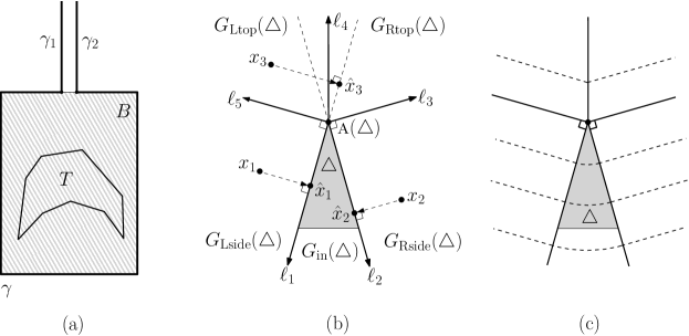
Figure 7: (a) The thick black curve $\gamma$ is a Hamiltonian curve of the abstract Voronoi diagram. (b) Five regions are defined by the five halflines from $\ell_{1}$ to $\ell_{5}$. The gray triangle is $\triangle$. (c) The dashed curves are contour curves with respect to $f_{\triangle}$.

5.3 Algorithm for Computing $\mathsf{rFVD}\cap T$

To compute the geodesic farthest-point Voronoi diagram restricted to $T$, we apply the algorithm in [11] that computes the abstract Voronoi diagram. Let $A$ be the set of all apexed triangles having their refined Voronoi cells on $\partial T$. In our problem, we regard the apexed triangles in $A$ as the sites. For two apexed triangles $\triangle_{1}$ and $\triangle_{2}$ in $A$, we define the bisecting curve $B(\triangle_{1},\triangle_{2})$ as the set $\{x\in\mathbb{R}^{2}:f_{\triangle_{1}}(x)=f_{\triangle_{2}}(x)\}$. The bisecting curve partitions $\mathbb{R}^{2}$ into two regions $D(\triangle_{1},\triangle_{2})$ and $D(\triangle_{2},\triangle_{1})$ such that $f_{\triangle_{1}}(x)>f_{\triangle_{2}}(x)$ for $x\in D(\triangle_{1},\triangle_{2})$ and $f_{\triangle_{2}}(x)>f_{\triangle_{1}}(x)$ for $x\in D(\triangle_{2},\triangle_{1})$. We denote the abstract Voronoi diagram for the apexed triangles by $\mathsf{aVD}$ and the cell of $\triangle\in A$ on $\mathsf{aVD}$ by $\mathsf{aCell}(\triangle)$.

To apply the algorithm in [11], we show that the family of the bisecting curves is admissible and Hamiltonian in the following subsection. We also prove that $\mathsf{aVD}\cap T$ is exactly $\mathsf{rFVD}\cap T$. After computing $\mathsf{aVD}$, we traverse $\mathsf{aVD}$ and extract $\mathsf{aVD}$ lying inside $T$. This takes $O(|\mathsf{rFVD}\cap\partial T|)$ time since no refined cell $\mathsf{rCell}(\triangle)$ contains a vertex of $T$ in its interior.

In addition, to apply the algorithm in [11], we have to choose a Hamiltonian curve $\gamma$. This algorithm requires $\gamma\cap\mathsf{aVD}$ to be given. To do this, we first choose an arbitrary box $B$ containing $T$. We compute one Voronoi cell of $\mathsf{aVD}$ directly in $O(|\mathsf{rFVD}\cap\partial T|)$ time by considering all apexed triangles in $A$. We also choose two arbitrary curves $\gamma_{1}$ and $\gamma_{2}$ with endpoints on the same edge of $\partial B$ which are contained in the Voronoi cell. See Figure 7(a). Then we can compute $\gamma$ consisting of $\gamma_{1},\gamma_{2}$ and a part of $\partial B$ such that $\gamma$ contains the four corners of $B$. Note that $\gamma$ is homeomorphic to a line. We will see that the order of the refined Voronoi cells along $\partial T$ coincides with the order of the Voronoi cells along $\partial B$ in $\mathsf{aVD}$ in Corollary 35. Therefore, we can obtain $\mathsf{aVD}\cap\gamma$ in $O(|\mathsf{rFVD}\cap\partial T|)$ time once we have $\mathsf{rFVD}\cap\partial T=\mathsf{aVD}\cap\partial T$.

5.4 Properties of Bisecting Curves and Voronoi Diagrams

5.4.1 $\mathsf{aVD}\cap T$ Coincides with $\mathsf{rFVD}\cap T$

Recall that $T$ is a lune-cell, which is bounded by a convex chain and a concave chain. Also, recall that the bottom side of every apexed triangle of $A$ is contained in $\partial T$. The following technical lemmas are used to prove that $\mathsf{rCell}(\triangle)\cap T$ coincides with $\mathsf{aCell}(\triangle)\cap T$ for any apexed triangle $\triangle\in A$. For a halfline $\ell$, we let $\bar{\ell}$ be the directed line containing $\ell$ with the same direction as $\ell$.

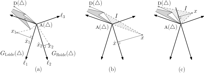
Figure 8: (a) If $\pi(x,\textsc{d}(\triangle))$ contains $\textsc{a}(\triangle)$, we have $g_{\triangle}(x)\leq d(\textsc{d}(\triangle),x)$. (b) Since $x$ lies in $G_{\mathrm{Rside}}(\triangle)$, the angle at $\textsc{a}(\triangle)$ is at least $\pi/2$, and thus $f_{\triangle}(x)<d(\textsc{d}(\triangle),x)$. (c) By triangle inequality, $f_{\triangle}(x)<d(\textsc{d}(\triangle),\hat{x})$. Also, we have $d(\textsc{d}(\triangle),\hat{x})<d(\textsc{d}(\triangle),x)$. Therefore we have $f_{\triangle}(x)<d(\textsc{d}(\triangle),x)$.

Lemma 25.

For any apexed triangle $\triangle$ of $A$, we have $f_{\triangle}(x)<d(\textsc{d}(\triangle),x)$ for any point $x$ such that $\pi(\textsc{d}(\triangle),x)$ contains $x^{\prime}$ with $f_{\triangle}(x^{\prime})<d(\textsc{d}(\triangle),x^{\prime})$.

Proof.

By definition, $d(\textsc{d}(\triangle),x)=d(\textsc{d}(\triangle),x^{\prime})+d(x,x^{\prime})$. Also, $f_{\triangle}(x)\leq f_{\triangle}(x^{\prime})+\|x-x^{\prime}\|$ by Lemma 24. Thus $f_{\triangle}(x)<d(\textsc{d}(\triangle),x^{\prime})+d(x,x^{\prime})=d(\textsc{d}(\triangle),x)$. ∎

Lemma 26.

For any apexed triangle $\triangle$ of $A$, we have $f_{\triangle}(x)\leq d(\textsc{d}(\triangle),x)$ for any point $x$ such that $\pi(\textsc{d}(\triangle),x)$ contains $\textsc{a}(\triangle)$. The equality holds if and only if $x$ lies in $\triangle$.

Proof.

If $x\in\triangle$, the lemma holds immediately. Thus we assume that $x$ is not in $\triangle$ and show that $f_{\triangle}(x)<d(\textsc{d}(\triangle),x)$. The Euclidean distance between $\textsc{a}(\triangle)$ and $\hat{x}$ is less than the Euclidean distance between $\textsc{a}(\triangle)$ and $x$. Since $d(\textsc{a}(\triangle),x)$ is at least their Euclidean distance, we have $f_{\triangle}(x)<d(\textsc{d}(\triangle),x)$. See Figure 8(a). ∎

Lemma 27.

For an apexed triangle $\triangle$ of $A$ such that the edge of $\pi(\textsc{a}(\triangle),\textsc{d}(\triangle))$ incident to $\textsc{a}(\triangle)$ lies to the left of $\bar{\ell}_{4}$, we have $f_{\triangle}(x)\leq d(\textsc{d}(\triangle),x)$ for any point $x\in T\setminus G_{\mathrm{Ltop}}(\triangle)$. The equality holds if and only if $x$ lies in $\triangle$.

Proof.

Let $x$ be a point in $T\setminus G_{\mathrm{Ltop}}(\triangle)$. If $\pi(\textsc{d}(\triangle),x)$ contains $\textsc{a}(\triangle)$, the lemma holds by Lemma 26. Thus we assume that $\pi(\textsc{d}(\triangle),x)$ does not contain $\textsc{a}(\triangle)$. Then $x$ does not lie in $G_{\mathrm{Lside}}(\triangle)$ since the maximal concave curve of $\partial T$ has angle-span at most $\pi/2$ by the assumption made in the beginning of this section and the angle at $\textsc{a}(\triangle)$ in $G_{\mathrm{Lside}}(\triangle)$ is $\pi/2$. See Figure 8(a). By construction of the apexed triangles and the assumption of the lemma, the edge of $\pi(\textsc{a}(\triangle),\textsc{d}(\triangle))$ incident to $\textsc{a}(\triangle)$ lies to the right of $\bar{\ell}_{2}$. Consider the interior $I$ of the geodesic convex hull of $\textsc{d}(\triangle)$, $\textsc{a}(\triangle)$ and $x$. Note that $\textsc{a}(\triangle)$ is a vertex of $I$.

Consider the case that $x$ is a vertex of $I$. Then $x$ lies in $G_{\mathrm{Rside}}(\triangle)\cup G_{\mathrm{Rtop}}(\triangle)$. If $x$ lies in $G_{\mathrm{Rside}}(\triangle)$, the angle at $\textsc{a}(\triangle)$ with respect to $I$ is at least $\pi/2$. Thus $d(\textsc{d}(\triangle),\hat{x})$ is at most $d(\textsc{d}(\triangle),x)$, and thus the lemma holds for this case. See Figure 8(b). If $x$ lies in $G_{\mathrm{Rtop}}(\triangle)$, we know that $f_{\triangle}(x)<d(\textsc{d}(\triangle),\hat{x})$ by triangle inequality, and $d(\textsc{d}(\triangle),\hat{x})<d(\textsc{d}(\triangle),x)$. Thus the lemma holds for this case. See Figure 8(c).

Now consider the case that $x$ is not a vertex of $I$. Let $x^{\prime}$ be the vertex of $I$ contained in $\pi(\textsc{a}(\triangle),x)$ which is closest to $x$. We can prove that $f_{\triangle}(x^{\prime})<d(\textsc{d}(\triangle),x^{\prime})$ as we did for the previous cases that $x$ is a vertex of $I$ since $x^{\prime}$ is a vertex of $I$. Then the lemma holds by Lemma 25. ∎

Lemma 28.

For an apexed triangle $\triangle$ of $A$ such that $\pi(\textsc{a}(\triangle),\textsc{d}(\triangle))$ does not overlap with the maximal concave curve of $\partial T$, we have $f_{\triangle}(x)\leq d(\textsc{d}(\triangle),x)$ for any point $x\in T$. The equality holds if and only if $x$ lies in $\triangle$.

Proof.

Without loss of generality, we assume that the edge of $\pi(\textsc{a}(\triangle),\textsc{d}(\triangle))$ incident to $\textsc{a}(\triangle)$ lies to the left of $\bar{\ell}_{4}$. By Lemma 27, the lemma holds, except for a point $x$ in $G_{\mathrm{Ltop}}(\triangle)$. Since $\pi(\textsc{a}(\triangle),\textsc{d}(\triangle))$ does not overlap with the maximal concave curve of $\partial T$, $\pi(x,\textsc{d}(\triangle))$ contains $\textsc{a}(\triangle)$ or a vertex $x^{\prime}$ of the maximal concave curve for any point $x$ in $G_{\mathrm{Ltop}}(\triangle)$. If $\pi(x,\textsc{d}(\triangle))$ contains $\textsc{a}(\triangle)$, the lemma holds by Lemma 26. Otherwise, $x^{\prime}$ lies on $G_{\mathrm{Rtop}}(\triangle)\cup G_{\mathrm{Rside}}(\triangle)$. Thus we have $f_{\triangle}(x^{\prime})<d(\textsc{d}(\triangle),x^{\prime})$. Therefore the lemma holds by Lemma 25. ∎

The following lemma implies that $\mathsf{aVD}\cap T$, that is the abstract Voronoi diagram of $A$ restricted to $T$, coincides with $\mathsf{rFVD}\cap T$.

Lemma 29.

For an apexed triangle $\triangle$ and a point $x\in T\cap\mathsf{rCell}(\triangle)$, $x$ lies in $\mathsf{aCell}(\triangle)$.

Proof.

Assume to the contrary that there are an apexed triangle $\triangle\in A$ and a point $x\in T\cap\mathsf{rCell}(\triangle)$ such that $x\notin\mathsf{aCell}(\triangle)$. This means that there is another apexed triangle $\triangle^{\prime}$ such that $f_{\triangle}(x)\leq f_{\triangle^{\prime}}(x)$. Among all such apexed triangles, we choose the one with the maximum $f_{\triangle^{\prime}}(x)$. Without loss of generality, we assume that the edge of $\pi(\textsc{a}(\triangle^{\prime}),\textsc{d}(\triangle^{\prime}))$ incident to $\textsc{a}(\triangle^{\prime})$ lies to the left of $\bar{\ell}_{4}$. We claim that $x$ lies in $G_{\mathrm{Ltop}}(\triangle^{\prime})$ and $\pi(\textsc{d}(\triangle^{\prime}),\textsc{a}(\triangle^{\prime}))$ overlaps with the maximal concave curve of $\partial T$, . Otherwise, we have $f_{\triangle^{\prime}}(x)\leq d(\textsc{d}(\triangle^{\prime}),x)$ by Lemmas 27 and 28. By definition, we have $f_{\triangle^{\prime}}(x)\leq d(\textsc{d}(\triangle^{\prime}),x)<d(\textsc{d}(\triangle),x)=f_{\triangle}(x)$, which is a contradiction.

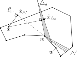
Figure 9: For $x$ lying in $T\cap G_{\mathrm{Ltop}}(\triangle^{\prime})$, $\|\hat{x}_{\triangle_{a}}-w\|<\|\hat{x}_{\triangle^{\prime}}-w\|$, and thus $f_{\triangle_{a}}(x)>f_{\triangle^{\prime}}(x)$.

In the following, we show that there is another apexed triangle $\triangle_{a}$ such that $f_{\triangle^{\prime}}(x)<f_{\triangle_{a}}(x)$. This is a contradiction as we chose the apexed triangle $\triangle^{\prime}$ with maximum $f_{\triangle^{\prime}}(x)$. Recall that we assume in the beginning of this section that $\triangle^{\prime}$ does not coincide with the closure of ${\mathsf{rCell}(\triangle^{\prime})}$. Let $w$ be $\textsc{a}(\triangle^{\prime})$ and $w^{\prime}$ be the clockwise neighbor of $w$ along $\partial T$. See Figure 9. In this case, there is another apexed triangle $\triangle_{a}$ such that $d(\textsc{d}(\triangle_{a}),w)>d(\textsc{d}(\triangle^{\prime}),w)$ and the bottom side of $\triangle_{a}$ is contained in $ww^{\prime}$. Otherwise, $w$ is in $\mathsf{rCell}(\triangle^{\prime})$, and thus $\triangle^{\prime}$ coincides with the closure of $\mathsf{rCell}(\triangle^{\prime})$, which is a contradiction. Let $\ell_{1}^{\prime}$ be the line containing the side of $\triangle^{\prime}$ which is closer to $w^{\prime}$ other than its bottom side. The point $\hat{x}_{\triangle_{a}}$ lies on the line passing through $w$ and $\textsc{a}(\triangle_{a})$. If it lies on the halfline starting from $w$ in direction opposite to $\textsc{a}(\triangle_{a})$, the claim holds immediately. Thus we assume that it lies on the halfline starting from $w$ in direction to $\textsc{a}(\triangle_{a})$. Then $x$ lies in the side of $\ell_{1}^{\prime}$ containing $w^{\prime}$ since $x\in G_{\mathrm{Ltop}}(\triangle)$. Moreover, $\hat{x}_{\triangle_{a}}$ and $x$ lie in different sides of $\ell_{1}^{\prime}$ since $\triangle_{a}$ has its bottom side on the line containing $ww^{\prime}$. Therefore, we have $\|w-\hat{x}_{\triangle_{a}}\|\leq\|w-\hat{x}_{\triangle^{\prime}}\|$. This implies that $f_{\triangle_{a}}(x)=d(\textsc{d}(\triangle_{a}),w)-\|w-\hat{x}_{\triangle_{a}}\|\geq d(\textsc{d}(\triangle_{a}),w)-\|w-\hat{x}_{\triangle^{\prime}}\|>d(\textsc{d}(\triangle^{\prime}),w)-\|w-\hat{x}_{\triangle^{\prime}}\|=f_{\triangle^{\prime}}(x)$, which is a contradiction. ∎

Corollary 30.

The abstract Voronoi diagram with respect to the functions $f_{\triangle}$ restricted to $T$ for all apexed triangles $\triangle\in A$ coincides with the refined geodesic farthest-point Voronoi diagram restricted to $T$.

5.4.2 The Family of Bisecting Curves is Admissible

Conditions 1 and 2 of Definition 22 hold due to Lemma 33. Condition 3A holds due to Lemmas 31 and 32. Condition 3B holds by the definition of the new distance function.

Lemma 31.

For an apexed triangle $\triangle$ in any subset $A^{\prime}$ of $A$, $\mathsf{aCell}(\triangle,A^{\prime})$ is connected.

Proof.

Here we use $\mathsf{aCell}(\triangle)$ to denote $\mathsf{aCell}(\triangle,A^{\prime})$ for an apexed triangle $\triangle\in A^{\prime}$. By Corollary 30, we have $\mathsf{rCell}(\triangle)\subseteq\mathsf{aCell}(\triangle)$. Assume to the contrary that there are at least two connected components of $\mathsf{aCell}(\triangle)$. Note that one of them contains $\mathsf{rCell}(\triangle)$.

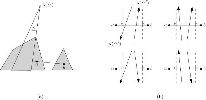
Figure 10: (a) There are two points $a$ and $b$ in different connected components of $\mathsf{aCell}(\triangle)$ (the gray region) such that $f_{\triangle}(a)=f_{\triangle}(b)$. (b) The arrows denote the position of $\textsc{a}(\triangle^{\prime})$ so that the functions $f_{\triangle^{\prime}}$ with domain $h_{1}$ is increasing, and $f_{\triangle^{\prime}}$ with domain $h_{3}$ is decreasing.

For any point $x\in\mathsf{aCell}(\triangle)$, there is a halfline from $x$ such that every point in the halfline, except $x$, has distance value $f_{\triangle}(\cdot)$ larger than $f_{\triangle}(x)$. This can be shown in a way similar to Lemma 4 together with Lemma 24. Thus there are two points $a$ and $b$ from different connected components of $\mathsf{aCell}(\triangle)$ such that $f_{\triangle}(a)=f_{\triangle}(b)$. See Figure 10(a).

Since $a$ and $b$ are in different connected components of $\mathsf{aCell}(\triangle)$, there is another triangle $\triangle^{\prime}$ in $A^{\prime}$ such that $f_{\triangle}(x)<f_{\triangle^{\prime}}(x)$ for some point $x\in ab$. Consider $f_{\triangle^{\prime}}$ restricted to the domain $ab$. Here, to make the description easier, we consider $ab$ as a line segment on $\mathbb{R}$, and each point on $ab$ as a real number. Without loss of generality, we assume that $a$ is smaller than $b$. If $G_{\mathrm{in}}(\triangle^{\prime})$ does not intersect $ab$, the function is linear in $ab$, and thus $f_{\triangle}(x)\geq f_{\triangle^{\prime}}(x)$ for any point $x\in ab$. This is a contradiction. Thus we assume that $G_{\mathrm{in}}(\triangle^{\prime})$ intersects $ab$.

We claim that $ab\setminus G_{\mathrm{in}}(\triangle^{\prime})$ consists of two connected components. If $G_{\mathrm{in}}(\triangle^{\prime})$ contains $ab$, the function $f_{\triangle^{\prime}}$ restricted to $ab$ is convex. Thus $f_{\triangle}(x)\geq f_{\triangle^{\prime}}(x)$ for any point $x\in ab$. If $G_{\mathrm{in}}(\triangle^{\prime})$ contains only one endpoint of $ab$, the function $f_{\triangle^{\prime}}$ restricted to $ab$ increases or decreases. Thus $f_{\triangle}(x)\geq f_{\triangle^{\prime}}(x)$ for any point $x\in ab$. Therefore, the claim holds.

Let $h_{1}$ and $h_{3}$ denote the connected components of $ab\setminus G_{\mathrm{in}}(\triangle^{\prime})$ containing $a$ and $b$, respectively. The function $f_{\triangle^{\prime}}$ with domain $h_{1}$ is increasing, and $f_{\triangle^{\prime}}$ with domain $h_{3}$ is decreasing. However, it is not possible. To see this, see Figure 10(b). There are four cases on the sides of $\triangle^{\prime}$: the clockwise angle from each side of $\triangle^{\prime}$ to $ab$ is at least $\pi/2$ or not. The arrows denote the position of $\textsc{a}(\triangle^{\prime})$ so that the function $f_{\triangle^{\prime}}$ with domain $h_{1}$ is increasing, and $f_{\triangle^{\prime}}$ with domain $h_{3}$ is decreasing. Each of the four cases makes a contradiction. Therefore, the lemma holds. ∎

Lemma 32.

For an apexed triangle $\triangle$ in any subset $A^{\prime}$ of $A$, $\mathsf{aCell}(\triangle,A^{\prime})$ is nonempty.

Proof.

Every apexed triangle $\triangle$ in $A$ has a refined Voronoi cell in $T$. Since $\mathsf{aCell}(\triangle,A^{\prime})$ contains $\mathsf{rCell}(\triangle)$, it is nonempty. ∎

Lemma 33.

For any two apexed triangles $\triangle_{1}$ and $\triangle_{2}$ in $A$, the set $\{x\in\mathbb{R}^{2}:f_{\triangle_{1}}(x)=f_{\triangle_{2}}(x)\}$ is a curve consisting of $O(1)$ algebraic curves.

Proof.

For any two apexed triangles $\triangle_{1}$ and $\triangle_{2}$, the set $\{x\in\mathbb{R}^{2}:f_{\triangle_{1}}(x)=f_{\triangle_{2}}(x)\}$ is a curve homeomorphic to a line by Lemma 31. Consider the subdivision of $\mathbb{R}^{2}$ by overlaying the two subdivisions as depicted in Figure 7(b), one from $\triangle_{1}$ and the other from $\triangle_{2}$. There are at most nine cells in the subdivision of $\mathbb{R}^{2}$. In each cell, $f_{\triangle_{1}}$ and $f_{\triangle_{2}}$ are algebraic functions. Thus, the set $\{x\in C:f_{\triangle_{1}}(x)=f_{\triangle_{2}}(x)\}$ is an algebraic curve for each cell $C$. ∎

5.4.3 The Family of Bisecting Curves is Hamiltonian

We show that $\gamma$ is a Hamiltonian curve. Recall that $B$ is a box containing $T$ and $\gamma$ is a curve that contains a part of $\partial B$ and is homeomorphic to a line. See Figure 7(a).

Lemma 34.

For every subset $A^{\prime}\subseteq A$ and $\triangle\in A^{\prime}$, $\mathsf{aCell}(\triangle,A^{\prime})$ is intersected by $\gamma$ exactly once.

Proof.

We claim that $\mathsf{aCell}(\triangle)$ is incident to $\partial B$ for any apexed triangle $\triangle\in A^{\prime}$. Since the halfline from a point $x$ in $\mathsf{rCell}(\triangle)$ in direction opposite to $\textsc{a}(\triangle)$ is contained in $\mathsf{rCell}(\triangle)$ and the bottom side of $\triangle$ is contained in $\mathsf{rCell}(\triangle)$, the region $G_{\mathrm{in}}(\triangle)\setminus\triangle$ is contained in $\mathsf{rCell}(\triangle)$, and thus is contained in $\mathsf{aCell}(\triangle)$. Since $G_{\mathrm{in}}(\triangle)\setminus\triangle$ intersects $\partial B$, all $\mathsf{aCell}(\triangle)$ are incident to $\partial B$.

We claim that $\mathsf{aCell}(\triangle)$ is intersected by $\partial B$ exactly once for every apexed triangle $\triangle\in A^{\prime}$. Otherwise, $\mathsf{rCell}(\triangle)$ intersects the boundary of $\partial T$ more than once since $\mathsf{aCell}(\triangle^{\prime})$ is connected and contains $\mathsf{rCell}(\triangle^{\prime})$ for every apexed triangle $\triangle^{\prime}\in A^{\prime}$. This contradicts the assumption made in the beginning of this section: $\mathsf{rCell}(\triangle)\cap\partial T$ is connected. Therefore, the claim holds.

For the part of $\gamma$ not contained in $\partial B$, recall that we chose $\gamma$ such that $\gamma\setminus\partial B$ is contained in $\mathsf{aCell}(\triangle^{\prime})$ for some $\triangle^{\prime}\in A^{\prime}$. Therefore, $\mathsf{aCell}(\triangle)$ is intersected by $\gamma$ exactly once. ∎

Corollary 35.

The order of $\mathsf{rCell}(\cdot)$ along $\partial T$ coincides with the order of $\mathsf{aCell}(\cdot,A)$ along $\partial B$.

5.5 Dealing with Cases Violating the Assumptions

In the previous subsections, we made the following four assumptions. Note that the last one is made in Subsection 5.2 for defining the distance function $f_{\triangle}(\cdot)$.

1. $T$ is a lune-cell.

2. $\mathsf{rCell}(\triangle)\cap\partial T$ is connected and contains the bottom side of $\triangle$ for any apexed triangle $\triangle$ with $\mathsf{rCell}(\triangle)\cap\partial T\neq\emptyset$.

3. If $\textsc{a}(\triangle)$ is on $\partial T$, the closure of $\mathsf{rCell}(\triangle)$ does not coincide with $\triangle$.

4. The maximal concave chain of $\partial T$ has angle-span at most $\pi/2$.

5. There is no pair $(\triangle_{1},\triangle_{2})$ of apexed triangles of $A$ such that two sides, one from $\triangle_{1}$ and the other from $\triangle_{2}$, are parallel.

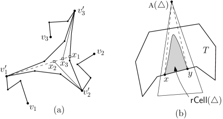
Figure 11: (a) The pseudo-triangle is subdivided into interior-disjoint four lune-cells. (b) We trim an apexed triangle $\triangle$ so that the bottom side of $\triangle$ is contained in $\mathsf{rCell}(\triangle)\cap\partial T$.

5.5.1 Satisfying Assumption 1

To satisfy Assumption 1, we subdivide each base cell further into subcells so that each subcell satisfies Assumption 1. For a pseudo-triangle $T$, we subdivide $T$ into four subcells as depicted in Figure 11(a). Let $v_{1},v_{2}$ and $v_{3}$ be three corners of $T$. Consider the three vertices $v_{1}^{\prime},v_{2}^{\prime},v_{3}^{\prime}$ of $T$ such that the maximal common path for $\pi(v_{i},v_{j})$ and $\pi(v_{i},v_{k})$ is $\pi(v_{i},v_{i}^{\prime})$ for $i=1,2,3$, where $j$ and $k$ are two distinct indices other than $i$.

First, we find a line segment $v_{1}^{\prime}x_{1}\subset T$ such that $v_{1}^{\prime}x_{1}\cap\partial T=\{v_{1}^{\prime},x_{1}\}$. Then, we find two line segments $v_{i}^{\prime}x_{i}\subset T$ such that $v_{i}^{\prime}x_{i}\cap\partial T=\{v_{i}^{\prime}\}$ and $x_{i}\in v_{1}^{\prime}x_{1}$ for $i=2,3$. This takes $O(|T|)=O(|\mathsf{rFVD}\cap\partial T|)$ time. Then the three line segments $v_{i}^{\prime}x_{i}$ subdivide $T$ into four lune-cells $T_{1},T_{2},T_{3}$ and $T_{4}$ for $i=1,2,3$. Note that to apply the algorithm in this section, $\mathsf{rFVD}\cap\partial T_{j}$ must be given. It can be computed in $O(|\mathsf{rFVD}\cap\partial T|)$ time by Corollary 19. Moreover, the total complexity of $\mathsf{rFVD}\cap\partial T_{j}$ for $j=1,2,3,4$ is $O(|\mathsf{rFVD}\cap\partial T|)$. Then we handle each lune-cell separately. Now every base cell is a lune-cell.

5.5.2 Satisfying Assumptions 2 and 3

We first subdivide each lune-cell $T$ further to satisfy the first part of Assumption 2 and Assumption 3 using a set of line segments with both endpoints on $\partial T$ as follows. For each endpoint $a$ of each connected component of $\mathsf{rCell}(\triangle)\cap\partial T$ for an apexed triangle $\triangle$ with $\mathsf{rCell}(\triangle)\cap\partial T\neq\emptyset$, we compute the ray from $a$ in direction opposite to $\textsc{a}(\triangle)$ that intersects $T$, it it exists, as we did in Phase 2 of the subdivision. By Lemma 4, each such ray is contained in the refined cell of its corresponding apexed triangle. Let $\mathcal{R}$ be the set of all such rays. If $\textsc{a}(\triangle)$ is in $\partial T$ and its $S$-farthest neighbor is $\textsc{d}(\triangle)$ for some apexed triangle $\triangle$, we also add the sides of $\triangle$ other than its bottom side to $\mathcal{R}$. We can obtain $\mathcal{R}$ in $O(|\mathsf{rFVD}\cap\partial T|+|T|)$ time as we did in Phase 2.

Then we subdivide $T$ with respect to the rays in $\mathcal{R}$. Since no ray in $\mathcal{R}$ intersects an arc of $\mathsf{rFVD}$ in $T$, the sum of $O(|\mathsf{rFVD}\cap\partial T^{\prime}|+|T^{\prime}|)$ for all subcells $T^{\prime}$ of $T$ is $O(|\mathsf{rFVD}\cap\partial T|)$. We can compute this subdivision in $O(|\mathsf{rFVD}\cap\partial T|+|T|)$ time. Moreover, each subcell is a lune-cell. The refined cell of every apexed triangle appears on each subcell at most once, and thus the first part of Assumption 2 is satisfied. Also, if $\textsc{a}(\triangle)$ is on $T$ and the closure of $\mathsf{rCell}(\triangle)$ is $\triangle$, we know that only one subcell $T^{\prime}$ intersects the interior of $\triangle$, and it coincides with $\triangle$. Thus we already know $\mathsf{rFVD}$ restricted to $T^{\prime}$, which is simply $\mathsf{rCell}(\triangle)$. Thus we do not need to apply the algorithm in this section. Therefore, every subcell $T^{\prime}$ such that we do not have $\mathsf{rFVD}$ restricted to $T^{\prime}$ yet satisfies Assumption 3. Also, these subcells still satisfy Assumption 1.

Then we decompose $\triangle$ into two triangles by the line passing through $\textsc{a}(\triangle)$ and $v$ for every $\triangle$ such that $\mathsf{rCell}(\triangle)\cap\partial T^{\prime}$ contains a convex vertex $v$ of a subcell $T^{\prime}$ (there are at most two such vertices). Note that $v$ lies in the interior of $P$ in this case. Only one of the triangles intersects the interior of $T^{\prime}$ by the definition of $T^{\prime}$. We replace $\triangle$ with the triangle. Then, $\mathsf{rCell}(\triangle)\cap\partial T^{\prime}$ is contained in an edge of $T^{\prime}$ for each apexed triangle $\triangle\in A$ if $\mathsf{rCell}(\triangle)\cap\partial T^{\prime}\neq\emptyset$. Let $x$ and $y$ be the two endpoints of $\mathsf{rCell}(\triangle)\cap\partial T^{\prime}$. See Figure 11(b). We trim $\triangle$ into the triangle whose corners are $x,y$ and $\textsc{a}(\triangle)$. From now on, when we refer an apexed triangle $\triangle$, we mean its trimmed triangle. Then $\mathsf{rCell}(\triangle)\cap T^{\prime}$ is still contained in $\triangle$ by Lemma 4. We do this for all apexed triangles. Every apexed triangle with $\mathsf{rCell}(\triangle)\cap\partial T^{\prime}\neq\emptyset$ has its bottom side on $\partial T^{\prime}$, and thus Assumption 2 is satisfied.

5.5.3 Satisfying Assumption 4

Since every base cell satisfies Assumptions 1,2 and 3, the maximal concave chain of each base cell has angle-span at most $\pi$ by the following lemma, but it is possible that the angle-span is larger than $\pi/2$.

Lemma 36.

For every base cell $T$ satisfying Assumptions 1,2 and 3, the maximal concave curve of $\partial T$ has angle-span at most $\pi$.

Proof.

Consider the maximal concave curve $\gamma$ of $\partial T$ and every apexed triangle $\triangle$ such that $\mathsf{rCell}(\triangle)$ intersects $\gamma$. The bottom sides of such apexed triangles are pairwise interior disjoint and are contained in $\gamma$ by the assumptions. Thus the apexed triangles can be sorted along $\gamma$ with respect to their bottom sides. Consider any two apexed triangles $\triangle_{1}$ and $\triangle_{2}$ appearing consecutively on the sorted list. There is an arc of $\mathsf{rFVD}$ induced by $(\triangle_{1},\triangle_{2})$ intersecting $\partial T$. Thus a side of $\triangle_{1}$ intersects a side of $\triangle_{2}$ at a point lying outside of $\gamma$. In other words, the interior of $\triangle_{1}$ intersects the interior of $\triangle_{2}$, or a side of one of $\triangle_{1}$ and $\triangle_{2}$ contains a side of the other triangle. Since this holds for every pair of consecutive apexed triangles along $\gamma$, the lemma holds. ∎

For each base cell $T$ whose maximal concave curve $\gamma$ has angle-span larger than $\pi/2$, we subdivide $T$ into at most three subcells so that the maximal concave curve of every subcell has angle-span at most $\pi/2$. While traversing $\gamma$ from one endpoint $v$ to the other endpoint $u$, we accumulate the turning angles at the vertices we traverse. Once the accumulated turning angle exceeds $\pi/2$ at a vertex $v^{\prime}$ of $\gamma$, we subdivide $T$ into three cells by the line through $v^{\prime}u^{\prime}$, where $u^{\prime}$ is the vertex next to $v^{\prime}$ along $\gamma$. Clearly, the part of $\gamma$ from $v$ to $v^{\prime}$ has angle-span at most $\pi/2$. The part of $\gamma$ from $u^{\prime}$ to $u$ also has angle-span at most $\pi/2$ by Lemma 36. Therefore, each of the three subcells has a maximal concave chain of angle-span at most $\pi/2$. As we did before, we compute $\mathsf{rFVD}\cap\partial T^{\prime}$ for every subcell $T^{\prime}$ in $O(|\mathsf{rFVD}\cap\partial T|+|T|)$ time in total. Then now every base cell still satisfies Assumptions 1 and 3, and the first part of Assumption 2. But it is possible that the second part of Assumption 2 is violated. In this case, we trim each apexed triangle again as we did before.

5.5.4 Satisfying Assumption 5

For every apexed triangle $\triangle$, we modify $f_{\triangle}(\cdot)$ as follows by defining $\hat{x}_{\triangle}$ differently. The algorithm [11] computes the abstract Voronoi diagram restricted to each side of a given Hamiltonian curve. In our case, it is sufficient to compute the abstract Voronoi diagram restricted to the side of $\gamma$ containing $T$. Thus, we restrict $f_{\triangle}(\cdot)$ to be defined in the side of $\gamma$ containing $T$.

First, we perturb $\ell_{3}$ and $\ell_{5}$ slightly such that $\ell_{3}$ and $\ell_{5}$ are circular arcs with common endpoint $\textsc{a}(\triangle)$ and the other endpoints on $\partial B$. We choose a sufficiently large number $r(\triangle)$ which is the common radius of $\ell_{3}$ and $\ell_{5}$. The rules for choosing $r(\triangle)$ will be described later. We let the center of $\ell_{3}$ lie on the halfline from $\textsc{a}(\triangle)$ in the direction opposite to $\ell_{1}$. Note that the center is fixed since the radius $r(\triangle)$ is fixed. Similarly, we let the center of $\ell_{5}$ lie on the halfline from $\textsc{a}(\triangle)$ in the direction opposite to $\ell_{2}$. See Figure 12(a). Then, for a point $x\in G_{\mathrm{Lside}}(\triangle)\cup G_{\mathrm{Ltop}}(\triangle)$, we map $x$ into the point $\hat{x}_{\triangle}$ on the line containing $\ell_{1}$ such that $r(\triangle)=\|\hat{x}_{\triangle}-c\|=\|x-c\|$, for some point $c$ on the halfline from $\textsc{a}(\triangle)$ in the direction opposite to $\ell_{1}$. Note that $\hat{x}_{\triangle}$ is unique. Similarly, we define $\hat{x}_{\triangle}$ for a point $x\in G_{\mathrm{Rside}}(\triangle)\cup G_{\mathrm{Rtop}}(\triangle)$. Now, each contour curve consists of three circular arcs. See Figure 12(b).

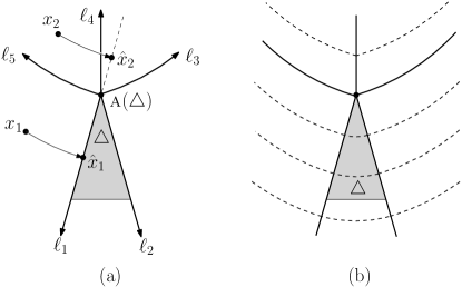
Figure 12: (a) The box $B$ is not depicted. Now $\ell_{3}$ and $\ell_{5}$ are circular arcs. (b) A contour curve consists of three circular arcs.

There are three rules with regard to choosing $r(\triangle)$: (1) $r(\triangle)\neq r(\triangle^{\prime})$ for any two distinct apexed triangles $\triangle$ and $\triangle^{\prime}$, (2) $r(\triangle)$ is larger than the diameters of $B$ and $P$ for every $\triangle$, and (3) for any two apexed triangles $\triangle$ and $\triangle^{\prime}$ such that the bottom side of $\triangle$ is contained in the maximal concave curve of $T$ and the bottom side of $\triangle^{\prime}$ is contained in the maximal convex curve of $T$, we have $r(\triangle)<r(\triangle^{\prime})$. We can choose $r(\triangle)$ for every apexed triangle $\triangle$ in time linear in the number of the apexed triangles in $A$. Here, we need Rule (1) to satisfy Lemma 33, Rule (2) to satisfy Lemmas 25, 26 and 27, and Rule (3) to satisfy Lemma 29.

All previous lemmas and corollaries, except Lemma 27, hold for the new distance function. For Lemma 27, we can prove that the clockwise angle from $\ell_{1}$ to the line passing through $\textsc{a}(\triangle)$ and $\ell_{5}\cap\partial B$ is at most a constant $\pi/\alpha$ depending only on the ratio between the maximum of $r(\triangle)$ and the diameter of $B$ (or $P$). Since we can choose the maximum of $r(\triangle)$ to be a constant times the diameter of $B$ (or $P$), we can regard this ratio as a constant. Then we replace $\pi/2$ with $\pi/\alpha$ in Assumption 4, and subdivide a base cell using at most $\alpha$ lines instead of subdividing it using only one line in Section 5.5.3. Then we can obtain base cells satisfying Assumption 4, and Lemma 27 holds. With the new distance function, we can compute $\mathsf{rFVD}\cap T$ without any assumptions in $O(|\mathsf{rFVD}\cap\partial T|+|T|)$ time.

Lemma 37.

Given a base cell $T$ constructed by the subdivision algorithm in Section 4.1, $\mathsf{rFVD}\cap T$ can be computed in $O(|\mathsf{rFVD}\cap\partial T|+|T|)$ time.

Remark on the space complexity.

By Lemma 15, $\mathsf{rFVD}$ restricted to all cells in the final iteration of Step 2 is of complexity $O(n\log\log n)$. Thus the space complexity is $O(n\log\log n)$. We can improve the space complexity to $O(n)$ as follows. When we recursively apply the subdivision of Step 2 to each cell, we give a specific order of the cells: when the recursion is completed for one cell, we apply the subdivision to one of its neighboring cells. Moreover, when we obtain a base cell, we apply Step 3 without waiting until Step 2 is completed. Assume that we complete the recursions for two adjacent cells. Then we have $\mathsf{rFVD}$ restricted to these cells. We merge two Voronoi diagrams and discard the information on the common boundary of these cells. In this way, the part of $\mathsf{rFVD}$ we have is of complexity $O(n)$ and the cells we maintain are of complexity $O(n)$ in total at any time. Therefore, we can compute $\mathsf{rFVD}$ in $O(n\log\log n)$ time using $O(n)$ space.

Theorem 38.

The geodesic farthest-point Voronoi diagram of the vertices of a simple $n$-gon can be computed in $O(n\log\log n)$ time using $O(n)$ space.

6 Sites Lying on the Boundary of a Simple Polygon

In this section, we show that the results presented in the previous sections are general enough to work for an arbitrary set $S$ of sites contained in the boundary of $P$. In this case, we assume without loss of generality that all sites of $S$ are vertices of $P$. This can be achieved by splitting each edge $uv$ that contain a site $s$ of $S$ into two, $us$ and $sv$, with a new vertex $s$.

We decompose the boundary of $P$ into chains of consecutive vertices that share the same $S$-farthest neighbor and edges of $P$ whose endpoints have distinct $S$-farthest neighbors. The following lemma is a counterpart of Lemma 7. Lemma 7 is the only place where it was assumed that $S$ is the set of vertices of $P$. The algorithm for computing a set of apexed triangles in [2] is based on Lemma 7. By replacing Lemma 7 with Lemma 39, this algorithm works for a set of sites on the boundary.

Lemma 39.

Given a set $S$ of $m$ sites contained in $\partial P$, we can compute the $S$-farthest neighbor of each vertex of $P$ in $O(n+m)$ time.

Proof.

Let $w:P\to\mathbb{R}$ be a real valued function on the vertices of $P$ such that for each vertex $v$ of $P$,

$$w(v)=\left\{\begin{array}[]{ll}D_{P}&\text{if $v\in S$}\\ 0&\text{otherwise,}\end{array}\right.$$

where $D_{P}$ is any fixed constant larger than the geodesic diameter of $P$. Recall that the diameter of $P$ can be computed in linear time [9].

For each vertex $v\in P$, we want to identify the $S$-farthest neighbor $\textsc{n}(v)$. To this end, we define a new distance function $d^{*}:P\times P\to\mathbb{R}$ such that for any two points $p$ and $q$ of $P$, $d^{*}(p,q)=d(p,q)+w(p)+w(q)$. Using a result from Hershberger and Suri [9, Section 6.1 and 6.3], we can compute the farthest neighbor of each vertex of $P$ with respect to $d^{*}$ in $O(n+m)$ time.

By the definition of the function $w$, the maximum distance from any vertex of $P$ is achieved at a site of $S$. Therefore, the farthest neighbor from a vertex $v$ of $P$ with respect to $d^{*}$ is indeed the $S$-farthest neighbor, $\textsc{n}(v)$, of $v$. ∎

Theorem 40.

The geodesic farthest-point Voronoi diagram of $m$ points on the boundary of a simple $n$-gon can be computed in $O((n+m)\log\log n)$ time.

6.1 Few Convex or Few Reflex Vertices

We can compute $\mathsf{FVD}[P,S]$ in $O((n+m)\log\log\min\{c,r\})$ time for a simple $n$-gon $P$ and a set $S$ of $m$ points on the boundary of $P$, where $c$ is the number of the convex vertices of $P$ and $r$ is the number of the reflex vertices of $P$. To achieve this, we apply two different algorithms depending on whether $r\geq c$ or $r<c$.

Few Convex Vertices.

In the case that $r\geq c$, we simply apply the algorithm in Theorem 40. We give a tighter analysis that the running time is $O((n+m)\log\log c)$. A basic observation is that the $\log\log n$ factor in the running time of Theorem 40 is the number of iterations of the subdivision in the second phase described in Section 4. In the second phase, we choose every $\lfloor\sqrt{t}\rfloor$th convex vertices of a $t$-path-cell along its boundary to subdivide the cell into $(\lfloor\sqrt{t}\rfloor+1)$-path-cells and base cells for some $t\in\mathbb{R}$. They recursively subdivide $t^{\prime}$-path-cells for $t^{\prime}>3$ until every cell becomes a $3$-path-cell or a base cell. Initially, we are given $P$ as a $c$-path-cell. This implies that the number of iterations of the subdivision is indeed $\log\log c$. Therefore, we can obtain $\mathsf{FVD}[P,S]$ in $O((n+m)\log\log\min\{c,r\})$ time if $r\geq c$.

Few Reflex Vertices.

We first compute $\mathsf{FVD}[P,S]$ restricted to the boundary of $P$ in $O(n+m)$ time using Theorem 9. Then we subdivide $P$ into a number of lune-cells and $r$-path-cells as follows. Recall that a lune-cell is a subpolygon of $P$ whose boundary consists of a convex chain and a concave chain. We compute the geodesic convex hull $\mathsf{CH}$ of the reflex vertices of $P$. The interior of $\mathsf{CH}$ consists of a number of connected regions. Note that each connected region has complexity $O(r)$. In other words, each connected region is an $r$-path-cell. Moreover, the total complexity of all connected regions is $O(r)$.

Consider the connected regions of $P\setminus\mathsf{CH}$. The boundary of each connected region consists of a part of the boundary of $\mathsf{CH}$ and a convex chain connecting some convex vertices of $P$ and sites of $S$. Thus, each connected region is a lune-cell. See Figure 13.

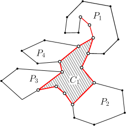
Figure 13: The geodesic convex hull (dashed region) of the reflex vertices of $P$ subdivides $P$ into lune-cells ($P_{i}$’s for $i=1,2,3,4$) and one $t$-path-cell ($C_{1}$).

We compute $\mathsf{FVD}$ restricted to the boundary of $\mathsf{CH}$ in $O(n+m)$ time using Lemma 20. Then for each $r$-path-cell, we apply the algorithm in Section 4 and compute $\mathsf{FVD}[P,S]$ restricted to the cell in total $O((n+m)\log\log r)$ time. For each lune-cell, we apply the algorithm in Section 5 and compute $\mathsf{FVD}[P,S]$ restricted to each cell. The total complexity of $\mathsf{FVD}$ restricted to all lune-cells and all $r$-path-cells is $O(n+m)$. Therefore, we can obtain $\mathsf{FVD}$ restricted to each lune-cell in $O(n+m)$ time in total. Since the cells are pairwise interior disjoint, we can obtain $\mathsf{FVD}[P,S]$ by simply combining all of them. Therefore, we can obtain $\mathsf{FVD}[P,S]$ in $O((n+m)\log\log\min\{c,r\})$ time if $r<c$, and we have the following theorem.

Theorem 41.

For a simple $n$-gon $P$ with $c$ convex vertices and $r$ reflex vertices, we can compute the farthest-point geodesic Voronoi diagram of a set of $m$ sites on the boundary of $P$ in $O((n+m)\log\log\min\{c,r\})$ time.

7 Sites Lying in a Simple Polygon

In this section, we consider a set $S$ of point sites lying in $P$. It is known that a site of $S$ appears on the boundary of the geodesic convex hull $\mathsf{CH}$ of $S$ if it has a nonempty Voronoi cell in $P$. Thus, we first compute $\mathsf{CH}$ in $O(n+m\log m)$ time [8]. Since the sites lying in the interior of $\mathsf{CH}$ do not have nonempty Voronoi cells, we remove them from $S$. Then every site of $S$ lies on the boundary of $\mathsf{CH}$.

Our algorithm consists of two steps. In the first step, we subdivide $P$ into three interior disjoint subpolygons, which we call funnels, in $O(n+m)$ time. The boundary of a funnel consists of two line segments and a part of the boundary of $P$. In the second step, we compute $\mathsf{FVD}[P,S]$ restricted to each funnel in $O((n+m)\log\log n)$ time. By merging them, we can obtain $\mathsf{FVD}[P,S]$ in $O((n+m)\log\log n)$ time excluding the time for computing $\mathsf{CH}$, or $O(n\log\log n+m\log m)$ time including the time for computing $\mathsf{CH}$.

7.1 Subdivision of $P$ into Three Funnels

We compute the geodesic center $g$ of $S$ with respect to $P$. Recall that it is the point in $P$ that minimizes the maximum geodesic distance to all sites of $S$. Moreover, it coincides with the geodesic center of $\mathsf{CH}$ with respect to $\mathsf{CH}$ [3, Corollary 2.3.5]. Ahn at al. [2] presented an algorithm to compute the geodesic center of a simple $n$-gon in $O(n)$ time. Since we have $\mathsf{CH}$, we can compute $g$ in $O(n+m)$ time.

We subdivide $P$ into three funnels with respect to $g$ as follows. There are at most three sites equidistant from $g$ by the general position assumption. Let $s_{1},s_{2}$ and $s_{3}$ be such sites sorted in clockwise order along the boundary of $\mathsf{CH}$. ($s_{3}$ might not exist.) While computing the center $g$, we can obtain such sites. For each $i=1,2,3$, we extend the edge of $\pi(g,s_{i})$ incident to the center $g$ towards $g$ until it escapes from $P$. Let $s_{i}^{\prime}$ be the point on $\partial P$ hit by this extension. See Figure 14(a). Then the three line segments $gs_{1}^{\prime},gs_{2}^{\prime}$ and $gs_{3}^{\prime}$ subdivide $P$ into three regions whose boundary consists of a part of $\partial P$ and two line segments sharing a common endpoint $g$. We call each region a funnel. We call the common boundary of $P$ and a funnel the bottom side of the funnel.

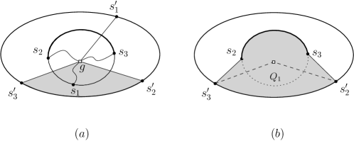
Figure 14: (a) The funnel $F_{1}$ (gray region). (b) There are some points $p,q\in Q_{1}$ such that the geodesic path between $p$ and $q$ restricted to lie in $Q_{1}$ is not the same as $\pi(p,q)$, the geodesic path between $p$ and $q$ restricted to lie in $P$.

We denote the funnel bounded by $gs_{2}^{\prime}$ and $gs_{3}^{\prime}$ by $F_{1}$. We denote the set of the sites of $S$ lying on the part of the boundary of $\mathsf{CH}$ from $s_{2}$ to $s_{3}$ in clockwise order by $S_{1}$. Similarly, we define $F_{2},F_{3}$ and $S_{2},S_{3}$. Note that $F_{i}$’s are pairwise interior disjoint.

We can compute $s_{1}^{\prime},s_{2}^{\prime}$ and $s_{3}^{\prime}$ in $O(\log n)$ time [6]. Therefore, we can obtain $F_{i}$ and $S_{i}$ for $i=1,2,3$ in $O(n+m)$ time in total. Now we consider a few properties of the funnels. By definition, the $S$-farthest neighbors of $g$ are $s_{1},s_{2}$ and $s_{3}$. Thus, $g$ lies on the common boundary of $\mathsf{Cell}(S,s_{i})$ for $i=1,2,3$. By Corollary 5, we have the following lemma.

Lemma 42.

The line segment $gs_{i}^{\prime}$ for $i=1,2,3$ is contained in $\mathsf{Cell}(S,s_{i})$.

Due to the following property, we can obtain $\mathsf{FVD}[P,S]$ by simply merging $\mathsf{FVD}[P,S_{i}]$ restricted to $F_{i}$ for $i=1,2,3$. We show how to compute $\mathsf{FVD}[P,S_{i}]$ restricted to $F_{i}$ in the following subsection.

Lemma 43.

For each $i=1,2,3$, every point in $F_{i}$ has its $S$-farthest neighbor in $S_{i}$.

Proof.

Aronov et al. [3] showed that $\mathsf{FVD}[P,S]$ forms a tree, that is, every nonempty Voronoi cell is incident to the boundary of $P$. Moreover, they showed that every Voronoi cell of $\mathsf{FVD}[P,S]$ is connected. By Lemma 42, $gs_{2}^{\prime}$ is contained in $\mathsf{Cell}(S,s_{2})$ and $gs_{3}^{\prime}$ is contained in $\mathsf{Cell}(S,s_{3})$. Therefore, for any site $s\in S$ with $\mathsf{Cell}(S,s)\cap F_{i}\neq\emptyset$, its Voronoi cell $\mathsf{Cell}(S,s)$ intersects the bottom side of $F_{i}$.

The ordering lemma states that the order of sites along the boundary of $\mathsf{CH}$ is the same as the order of Voronoi cells along $\partial P$. Therefore, a site $s$ whose Voronoi cell intersects the bottom side of $F_{i}$ is in $S_{i}$. Thus, the lemma holds. ∎

The following property is used to compute $\mathsf{FVD}[P,S_{i}]$ restricted to $F_{i}$ for $i=1,2,3$ in the following section.

Lemma 44.

For each funnel $F_{i}$, there are two points $p_{1},p_{2}\in\partial P$ such that $\pi(p_{1},p_{2})$ separates $F_{i}$ and $S_{i}$.

Proof.

Since $g$ is the geodesic center of $\mathsf{CH}$, there are two points, $q_{1}$ and $q_{2}$, on the boundary of $\mathsf{CH}$ such that $\pi(q_{1},q_{2})$ contains $g$ and $\pi(q_{1},q_{2})$ separates $\{s_{2},s_{3}\}$ and $\{s_{1}\}$. Otherwise, we can move the position of $g$ slightly to reduce $d(g,s_{i})$ for all $i=1,2,3$, which contradicts that $g$ is the geodesic center of $\mathsf{CH}$ and $s_{i}$’s are the $S$-farthest neighbors of $g$. Note that one part of $\mathsf{CH}$ bounded by $\pi(q_{1},q_{2})$ contains all of $\pi(g,s_{2}),\pi(g,s_{3})$ and $S_{1}$.

We extend the edge of $\pi(q_{1},q_{2})$ incident to $q_{j}$ towards $q_{j}$ until it escapes from $P$, and let $p_{j}$ be the point on $\partial P$ hit by the extension for each $j=1,2$. Then $\pi(p_{1},p_{2})$ contains $\pi(q_{1},q_{2})$, and therefore a part of $P$ bounded by $\pi(p_{1},p_{2})$ contains $\pi(g,s_{2})$, $\pi(g,s_{3})$ and $S_{1}$. Thus, $gs_{3}^{\prime}$ and $gs_{2}^{\prime}$ are contained in the other part of $P$ bounded by $\pi(p_{1},p_{2})$, and so does $F_{1}$. This means that $\pi(p_{1},p_{2})$ separates $F_{1}$ and $S_{1}$. The argument also works for the other pairs of $F_{i}$ and $S_{i}$ for $i=2,3$ analogously. ∎

7.2 Computing $\mathsf{FVD}$ Restricted to Each Funnel

Consider $F_{1}$ and $S_{1}$. We can handle $F_{i}$ and $S_{i}$ for $i=2,3$ analogously. We want to compute $\mathsf{FVD}[P,S_{1}]$ restricted to $F_{1}$. The algorithm in Theorem 40 requires all sites to lie on the boundary of a simple polygon. However, in our case, some sites of $S_{1}$ may not lie on the boundary of $P$. Our general strategy is to construct three pairs $(P_{j},S_{j})$ of subpolygons $P_{j}$ of $P$ and subsets $S_{j}$ of $S$ with $j=a,b,c$ such that the sites of $S_{j}$ lie on the boundary of $P_{j}$. Then we apply the algorithm in Theorem 40 to each pair $(P_{j},S_{j})$ and compute the geodesic farthest-point Voronoi diagram restricted to $P_{j}$. We show that we can obtain $\mathsf{FVD}[P,S_{1}]$ restricted to $F_{1}$ by combining the diagrams.

Consider the subpolygon $Q_{1}$ of $P$ whose boundary consists of the bottom side of $F_{1}$, $\pi(s_{2}^{\prime},s_{3})$, $\pi(s_{3}^{\prime},s_{2})$ and the part of $\mathsf{CH}$ from $s_{2}$ to $s_{3}$ in clockwise order. See Figure 14(b). Note that all sites of $S_{1}$ are on the boundary of $Q_{1}$. However, applying the algorithm in Theorem 40 with input polygon $Q_{1}$ may not give a correct diagram in this case. This is because there are points $p,q\in Q_{1}$ such that the geodesic path between $p$ and $q$ is not contained in $Q_{1}$.

To avoid this, we consider the geodesic convex hull $H_{1}$ of $Q_{1}$ instead. See Figure 15(a). Since $Q_{1}$ is a simple polygon contained in $P$, we can compute $H_{1}$ in $O(n+m)$ time [18]. Let $t_{2}$ and $t_{3}$ be the sites of $S$ such that $\pi(s_{3}^{\prime},t_{2})$ and $\pi(s_{2}^{\prime},t_{3})$ lie on the boundary of $H_{1}$ and intersect $\mathsf{CH}$ only at $t_{2}$ and $t_{3}$, respectively. There exist such two points by Lemma 44. Note that $H_{1}$ contains the geodesic path of any two points lying in $H_{1}$.

Recall that our goal is to compute $\mathsf{FVD}[P,S_{1}]$ restricted to $F_{1}$. It coincides with $\mathsf{FVD}[H_{1},S_{1}]$ restricted to $F_{1}$ since $H_{1}$ contains the geodesic path of any two points in $H_{1}$ and contains both $S_{1}$ and $F_{1}$. However, there might be some sites of $S_{1}$ in the interior of $H_{1}$.

Observation 45.

$\mathsf{FVD}[P,S_{1}]$ restricted to $F_{1}$ coincides with $\mathsf{FVD}[H_{1},S_{1}]$ restricted to $F_{1}$.

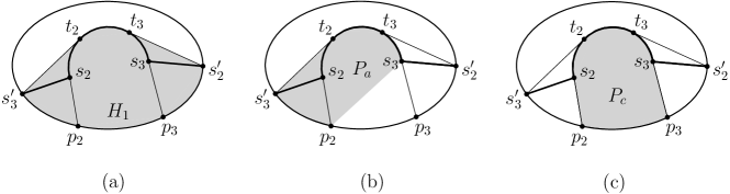
Figure 15: (a) The gray region $H_{1}$ contains the geodesic paths of any two points in $H_{1}$ and contains both $S_{1}$ and $F_{1}$. (b) Every point in $P_{a}\setminus P_{c}$ has its $S_{1}$-farthest neighbor on $\mathsf{CH}[t_{2},s_{3}]\cup\{s_{2}\}$. (c) The boundary of $P_{c}$ contains all sites of $S_{1}$.

We consider three subpolygons $P_{j}$ of $H_{1}$ associated with site sets $S_{j}$ with $j=a,b,c$ whose union is $H_{1}$. We will see that every site in $S_{j}$ lies on the boundary of $P_{j}$. For any two sites $s$ and $s^{\prime}$ in $S_{1}$, we use $\mathsf{CH}[s,s^{\prime}]$ to denote the part of the boundary of $\mathsf{CH}$ lying from $s$ to $s^{\prime}$ in clockwise order. Similarly, for any two points $p$ and $p^{\prime}$ on the boundary of $P$, we use $P[p,p^{\prime}]$ to denote the part of $\partial P$ lying from $p$ to $p^{\prime}$ in clockwise order.

Consider $\mathsf{CH}[s_{2},s_{3}]$. We extend its two edges of adjacent to $s_{2}$ and to $s_{3}$ towards $s_{2}$ and $s_{3}$ until they escape from $P$ at points $p_{2}$ and $p_{3}$ of $\partial P$, respectively. If $p_{2}$ or $p_{3}$ does not lie on the bottom side of $F_{1}$, we simply set $p_{2}=s_{3}^{\prime}$ or $p_{3}=s_{2}^{\prime}$, respectively. See Figure 15(a).

Lemma 46.

The four points $s_{2}^{\prime},p_{3},p_{2}$ and $s_{3}^{\prime}$ lie on the boundary of $\partial P$ in clockwise order.

Proof.

Lemma 44 implies that $\pi(s_{3}^{\prime},s_{2}^{\prime})$ intersects $s_{2}p_{2}$. Let $p_{2}^{\prime}$ be an intersection point. Consider the clockwise angle from the line segment $p_{2}^{\prime}s_{2}$ to the edge of $\pi(p_{2}^{\prime},s_{2}^{\prime})$ incident to $p_{2}^{\prime}$. This angle must be less than $\pi/2$. Otherwise, we have $d(s_{2}^{\prime},s^{\prime})>d(s_{2}^{\prime},s_{2})$ by [16, Corollary 2], where $s^{\prime}$ is the clockwise neighbor of $s_{2}$ along the boundary of $\mathsf{CH}$. This contradicts to the definition of $s_{2}^{\prime}$. The same holds for $s_{3}^{\prime}$ with respect to the intersection point $p_{3}^{\prime}$ of $\pi(s_{2}^{\prime},s_{3}^{\prime})$ with $s_{3}p_{3}$ and the counterclockwise neighbor of $s_{3}$.

Now we claim that $s_{2}p_{2}$ and $s_{3}p_{3}$ does not intersect each other. Assume to the contrary that they intersect each other at $x$. Since $\pi(s_{3}^{\prime},s_{2}^{\prime})$ separates $s_{2}$ and $s_{3}$ from $p_{2}$ and $p_{3}$, there are two cases: either $x$ lies in the subpolygon of $P$ induced by $\pi(s_{3}^{\prime},s_{2}^{\prime})$ in which $s_{2}$ and $s_{3}$ lie or not. See Figure 16(a-b). In any case, consider the pseudo-triangle with three corners $x,p_{2}^{\prime}$ and $p_{3}^{\prime}$. The path $\pi(p_{3}^{\prime},p_{2}^{\prime})$ is a concave chain with respect to this pseudo-triangle. This contradicts that the angles at $p_{3}^{\prime}$ and $p_{2}^{\prime}$ are less than $\pi/2$. Therefore, the claim holds, and the four points $s_{2}^{\prime},p_{3},p_{2}$ and $s_{3}^{\prime}$ lie on the boundary of $\partial P$ in clockwise order. ∎

Let $P_{a}$ be the subpolygon of $H_{1}$ whose boundary consists of $\mathsf{CH}[t_{2},s_{3}]$, $\pi(s_{3},p_{2})$, $P[p_{2},s_{3}^{\prime}]$ and $\pi(s_{3}^{\prime},t_{2})$. See Figure 15(b). Similarly, let $P_{b}$ be the subpolygon of $H_{1}$ whose boundary consists of $\mathsf{CH}[s_{2},t_{3}]$, $\pi(t_{3},s_{2}^{\prime})$, $P[s_{2}^{\prime},p_{3}]$ and $\pi(p_{3},s_{2})$. Let $P_{c}$ be the subpolygon of $H_{1}$ whose boundary consists of $\mathsf{CH}[s_{2},s_{3}]$, $s_{3}p_{3}$, $P[p_{3},p_{2}]$ and $p_{2}s_{2}$. See Figure 15(c).

Lemma 47.

Every point in $P_{a}\setminus P_{c}$ has its $S_{1}$-farthest neighbor on $\mathsf{CH}[t_{2},s_{3}]\cup\{s_{2}\}$. Similarly, every point in $P_{b}\setminus P_{c}$ has its $S_{1}$-farthest neighbor on $\mathsf{CH}[s_{2},t_{3}]\cup\{s_{3}\}$.

Proof.

We prove only the first part of the lemma. The second part can be proved analogously. We claim that the $S_{1}$-farthest neighbor of $p_{2}$ is in $\mathsf{CH}[t_{2},s_{3}]$. If the claim is true, every point in $P[p_{2},s_{3}^{\prime}]$ has its $S_{1}$-farthest neighbor on $\mathsf{CH}[t_{2},s_{3}]$ due to the ordering lemma [3, Corollary 2.7.4]. Moreover, every point on $\pi(s_{3}^{\prime},t_{2})$, $\mathsf{CH}[t_{2},t_{3}]$, and $\pi(t_{3},s_{2}^{\prime})$ has its $S_{1}$-farthest neighbor on $\mathsf{CH}[t_{2},s_{3}]\cup\{s_{2}\}$ due to the ordering lemma and the definition of $s_{3}^{\prime}$ and $s_{2}^{\prime}$. Due to Corollary 5, every point in $P_{a}\setminus P_{c}$ has its $S_{1}$-farthest neighbor on $\mathsf{CH}[t_{2},s_{3}]\cup\{s_{2}\}$.

To prove the claim, assume to the contrary that the $S_{1}$-farthest neighbor of $p_{2}$ is in $\mathsf{CH}[s_{2},t_{2}]\setminus\{t_{2}\}$. To make the description easier, we assume that $p_{2}s_{2}$ is vertical. See Figure 16(c). We first observe that $\mathsf{CH}[s_{2},t_{2}]$ is a convex chain with respect to $\mathsf{CH}$. If it is not true, there is some vertex of $P$ that appears on $\mathsf{CH}[s_{2},t_{2}]\setminus\{t_{2}\}$, and $\pi(s_{3}^{\prime},t_{2})$ overlaps with $\mathsf{CH}[s_{2},t_{2}]$ at the vertex, which contradicts that $\pi(s_{3}^{\prime},t_{2})$ intersects $\mathsf{CH}$ only at $t_{2}$.

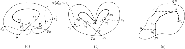
Figure 16: (a,b) If $s_{2}p_{2}$ and $s_{3}p_{3}$ intersect at $x$, the angles at $p_{3}^{\prime}$ and $p_{2}^{\prime}$ are at least $\pi/2$. (c) The proof of Lemma 46 implies that $s_{3}^{\prime}$ lies on $P[p_{2},p^{\prime\prime}]$. However, since $\pi(s_{3}^{\prime},t_{2})$ intersects $\mathsf{CH}$ only at $t_{2}$, the point $s_{3}^{\prime}$ lies on $P[s^{\prime},p_{2}]$, which is a contradiction.

Since $\mathsf{CH}[s_{2},t_{2}]$ is a convex chain and $t_{2}$ is not the $S_{1}$-farthest neighbor of $p_{2}$, $t_{2}$ is not the highest point of the chain. Let $s^{\prime}$ be the first point on $\partial P$ hit by the ray from the highest point $s$ of the chain going to the left horizontally. Since $\pi(s_{3}^{\prime},t_{2})$ intersects $\mathsf{CH}$ only at $t_{2}$, the point $s_{3}^{\prime}$ lies on $P[s^{\prime},p_{2}]$.

Now, as we did in the proof of Lemma 46, we consider an intersection point $p_{2}^{\prime}$ between $\pi(s_{3}^{\prime},s_{2}^{\prime})$ and $s_{2}p_{2}$. We already showed that the clockwise angle from the line segment $p_{2}^{\prime}s_{2}$ to the edge of $\pi(p_{2}^{\prime},s_{2}^{\prime})$ incident to $p_{2}^{\prime}$ is less than $\pi/2$. Thus, the counterclockwise angle from $p_{2}^{\prime}s_{2}$ to the edge of $\pi(p_{2}^{\prime},s_{3}^{\prime})$ incident to $p_{2}^{\prime}$ is larger than $\pi/2$. Let $p$ be the first point on $\partial P$ hit by the ray from $p_{2}^{\prime}$ going to the left horizontally. Since the counterclockwise angle is larger than $\pi/2$, the point $s_{3}^{\prime}$ lies on $P[p_{2},p]$.

Since $s$ is the highest point of $\mathsf{CH}[s_{2},t_{2}]$, the three points $p_{2},p$ and $s^{\prime}$ lie on the boundary of $P$ in clockwise order. Therefore, $P[s^{\prime},p_{2}]$ and $P[p_{2},p]$ are interior disjoint, which is a contradiction. Therefore, the claim holds. ∎

Moreover, the proof of this lemma implies the following corollary.

Corollary 48.

There is no point in $F_{1}\cap(P_{a}\setminus P_{c})$ whose $S_{1}$-farthest neighbor is $s_{2}$. Similarly, there is no point in $F_{1}\cap(P_{b}\setminus P_{c})$ whose $S_{1}$-farthest neighbor is $s_{3}$.

After obtaining $P_{a},P_{b}$ and $P_{c}$ in $O(n+m)$ time, we compute $\mathsf{FVD}[H_{1},S_{1}]$ restricted to $F_{1}$ as follows. For $\mathsf{FVD}[P_{c},S_{1}]$, we use the fact that all sites of $S_{1}$ lie on the boundary of $P_{c}$. Since $P_{c}$ has $O(n)$ reflex vertices, we can compute $\mathsf{FVD}[P_{c},S_{1}]$ in $O((n+m)\log\log n)$ time using Theorem 41. Then we cut $\mathsf{FVD}[P_{c},S_{1}]$ along the boundary of $F_{1}$. Recall that $F_{1}$ is a subpolygon of $S_{1}$ bounded by two line segments. Moreover, each line segment is contained in $\mathsf{Cell}(S,s_{i})$ for $i=2,3$. Thus, we can cut $\mathsf{FVD}[P_{c},S_{1}]$ along these line segments and obtain $\mathsf{FVD}[P_{c},S_{1}]$ restricted to $F_{1}$ in $O(n+m)$ time once we have $\mathsf{FVD}[P_{c},S_{1}]$.

For $\mathsf{FVD}[P_{a}\setminus P_{c},S_{1}]$ restricted to $F_{1}$, we use the fact that it coincides with $\mathsf{FVD}[P_{a},S_{a}]$ restricted to $F_{1}\cap(P_{a}\setminus P_{c})$, where $S_{a}$ is the set of sites of $S$ lying on $\mathsf{CH}[t_{2},s_{3}]$, which follows from Lemma 47 and Corollary 48. Note that all sites of $S_{a}$ lie on the boundary of $P_{a}$. Therefore, we can compute $\mathsf{FVD}[P_{a},S_{a}]$ in $O((n+m)\log\log n)$ time by Theorem 41. Since we already have $\mathsf{FVD}[P_{c},S_{1}]$ restricted to $F_{1}$, we can obtain the part of $\mathsf{FVD}[P_{a},S_{a}]$ restricted to $F_{1}\cap(P_{a}\setminus P_{c})$ in $O(n+m)$ by cutting $\mathsf{FVD}[P_{a},S_{a}]$ along the boundaries of $P_{c}$ and $F_{1}$. Similarly, we can compute $\mathsf{FVD}[P_{b}\setminus P_{c},S_{1}]$ restricted to $F_{1}$ in the same time.

Since $P_{c}$, $P_{a}\setminus P_{c}$ and $P_{b}\setminus P_{c}$ are pairwise interior disjoint, we can combine the three Voronoi diagrams easily and obtain $\mathsf{FVD}[H_{1},S_{1}]$ restricted to $F_{1}$ in $O(n+m)$ time. Recall that our goal in this subsection is to compute $\mathsf{FVD}[P,S_{1}]$ restricted to $F_{1}$. By Observation 45, it is equivalent to $\mathsf{FVD}[H_{1},S_{1}]$ restricted to $F_{1}$. Since $\mathsf{FVD}[H_{1},S_{1}]$ restricted to $F_{1}$ can be computed in $O((n+m)\log\log n)$ time, we can compute $\mathsf{FVD}[P,S]$ in $O((n+m)\log\log n+m\log m)$ time in total including the time for computing the geodesic convex hull $\mathsf{CH}$ of the sites. For $n=O(m)$, we have $m\log\log n=O(m\log m)$. For $n=\Omega(m)$, we have $m\log\log n=O(n\log\log n)$. Therefore, we have the following theorem.

Theorem 49.

The farthest-point geodesic Voronoi diagram of $m$ points in a simple $n$-gon can be computed in $O(n\log\log n+m\log m)$ time.

References

- Aggarwal et al. [1989] A. Aggarwal, L. J. Guibas, J. Saxe, and P. W. Shor. A linear-time algorithm for computing the Voronoi diagram of a convex polygon. Discrete & Computational Geometry, 4(6):591–604, 1989.
- Ahn et al. [2016] H.-K. Ahn, L. Barba, P. Bose, J.-L. Carufel, M. Korman, and E. Oh. A linear-time algorithm for the geodesic center of a simple polygon. Discrete Comput. Geom., 56(4):836–859, 2016.
- Aronov et al. [1993] B. Aronov, S. Fortune, and G. Wilfong. The furthest-site geodesic Voronoi diagram. Discrete & Computational Geometry, 9(3):217–255, 1993.
- Asano and Toussaint [1985] T. Asano and G. Toussaint. Computing the geodesic center of a simple polygon. Technical Report SOCS-85.32, McGill University, 1985.
- Chazelle [1982] B. Chazelle. A theorem on polygon cutting with applications. In Proceedings of the 23rd Annual Symposium on Foundations of Computer Science (FOCS 1982), pages 339–349, 1982.
- Chazelle et al. [1994] B. Chazelle, H. Edelsbrunner, M. Grigni, L. Guibas, J. Hershberger, M. Sharir, and J. Snoeyink. Ray shooting in polygons using geodesic triangulations. Algorithmica, 12(1):54–68, 1994.
- Guibas et al. [1987] L. Guibas, J. Hershberger, D. Leven, M. Sharir, and R. Tarjan. Linear-time algorithms for visibility and shortest path problems inside triangulated simple polygons. Algorithmica, 2(1):209–233, 1987.
- Guibas and Hershberger [1989] L. J. Guibas and J. Hershberger. Optimal shortest path queries in a simple polygon. Journal of Computer and System Sciences, 39(2):126–152, 1989.
- Hershberger and Suri [1997] J. Hershberger and S. Suri. Matrix searching with the shortest-path metric. SIAM Journal on Computing, 26(6):1612–1634, 1997.
- Klein [1989] R. Klein. Concrete and abstract Voronoi diagrams. Springer-Verlag Berlin Heidelberg, 1989.
- Klein and Lingas [1994] R. Klein and A. Lingas. Hamiltonian abstract Voronoi diagrams in linear time. In Prooceedings of the 5th International Symposium on Algorithms and Computation (ISAAC 1994), pages 11–19. Springer Berlin Heidelberg, 1994.
- Mitchell [2000] J. S. B. Mitchell. Geometric shortest paths and network optimization. In Handbook of Computational Geometry, pages 633–701. Elsevier, 2000.
- Oh and Ahn [2017] E. Oh and H.-K. Ahn. Voronoi diagrams for a moderate-sized point-set in a simple polygon. In Proceedings of the 33rd International Symposium on Computational Geometry (SoCG 2017), volume 77, pages 52:1–52:15. Schloss Dagstuhl–Leibniz-Zentrum für Informatik, 2017.
- Oh et al. [2016] E. Oh, L. Barba, and H.-K. Ahn. The farthest-point geodesic Voronoi diagram of points on the boundary of a simple polygon. In Proceedings of the 32nd International Symposium on Computational Geometry (SoCG 2016), volume 51, pages 56:1–56:15. Schloss Dagstuhl–Leibniz-Zentrum für Informatik, 2016.
- Papadopoulou [1999] E. Papadopoulou. -pairs non-crossing shortest paths in a simple polygon. International Journal of Computational Geometry and Applications, 9(6):533–552, 1999.
- Pollack et al. [1989] R. Pollack, M. Sharir, and G. Rote. Computing the geodesic center of a simple polygon. Discrete & Computational Geometry, 4(6):611–626, 1989.
- Suri [1989] S. Suri. Computing geodesic furthest neighbors in simple polygons. Journal of Computer and System Sciences, 39(2):220–235, 1989.
- T. [1986] T. G. T. An optimal algorithm for computing the relative convex hull of a set of points in a polygon. In Proceeding of EURASIP-86, Part 2, pages 853–856, 1986.