Approximations to galaxy star formation rate histories: properties and uses of two examples

Abstract

Galaxies evolve via a complex interaction of numerous different physical processes, scales and components. In spite of this, overall trends often appear. Simplified models for galaxy histories can be used to search for and capture such emergent trends, and thus to interpret and compare results of galaxy formation models to each other and to nature. Here, two approximations are applied to galaxy integrated star formation rate histories, drawn from a semi-analytic model grafted onto a dark matter simulation. Both a lognormal functional form and principal component analysis (PCA) approximate the integrated star formation rate histories fairly well. Machine learning, based upon simplified galaxy halo histories, is somewhat successful at recovering both fits. The fits to the histories give fixed time star formation rates which have notable scatter from their true final time rates, especially for quiescent and “green valley” galaxies, and more so for the PCA fit. For classifying galaxies into subfamilies sharing similar integrated histories, both approximations are better than using final stellar mass or specific star formation rate. Several subsamples from the simulation illustrate how these simple parameterizations provide points of contact for comparisons between different galaxy formation samples, or more generally, models. As a side result, the halo masses of simulated galaxies with early peak star formation rate (according to the lognormal fit) are bimodal. The galaxies with a lower halo mass at peak star formation rate appear to stall in their halo growth, even though they are central in their host halos.

1 Introduction

Many galaxy properties are now observed and measured in samples extending over huge volumes of sky, reaching back to earlier and earlier times. Several trends have been discovered to emerge from all the interrelated complexities of galaxy formation. These include the fact that small isolated galaxies tend to be star forming, central galaxies in large dark matter halos tend to be quiescent, and galaxies of a certain stellar mass often inhabit host dark matter halos of a certain mass. Finding these and other trends can help identify and understand physical causes and effects in galaxy formation. For instance, several such trends are thought to originate from self-regulation of physical processes, so that tracking one process implies the behavior of others (for example, Schaye et al (2010); Hopkins, Quataert & Murray (2011)). Simple models can be used to try to identify such trends. These trends can also help to guide the construction of simple models, especially when they have simple physical interpretations, such as the stellar mass-halo mass relations.

Here, the focus is on simple descriptions of (integrated) galaxy histories rather than fixed time properties. These descriptions can provide a point of contact between results of detailed models (arising from the interplay of all the model processes and components) and observations, or between two different models. Again, these descriptions can also encode known trends, and help to search for new ones. For instance, galaxy halo histories on average can be fit by a simple parameterized form (e.g., Wechsler et al (2002); Zhao et al (2003); Tasitsiomi et al (2004); McBride, Fakhouri & Ma (2009); Zhao et al (2009); Dekel et al (2013); Rodriguez-Puebla et al (2017) and many others). Several of these halo history parameterizations incorporate the physical insight that galaxy halos often have a quickly growing phase, dominated by significant mergers, followed by a slower accretion dominated phase. That is, the functional form of the simplified models allow a physical interpretation as well.

In the following, two simplified descriptions of integrated galaxy star formation rate histories are applied to several samples constructed from the L-galaxies semi-analytic model (Henriques et al, 2015). The N-body Millennium simulation (Springel et al, 2005; Lemson et al, 2006; Angulo & White, 2010; Angulo & Hilbert, 2015) provides the underlying halo and subhalo histories. One description is based upon an integrated lognormal fit, following the proposal studied in detail in Gladders et al (2013); Abramson et al (2016); Diemer et al (2017). A specific physical shape is assumed. The second description follows Cohn & Van de Voort (2015); Sparre et al (2015), applying principal component analysis (PCA), not to the instantaneous star formation rate histories (as in those works) but instead to the integrated star formation rate histories. PCA uses fluctuations around the sample average history, determined by the sample. PCA thus incorporates all of a sample’s galaxy histories in its definition, in addition to assigning parameters to each galaxy’s individual history. Using integrated rather than instantaneous star formation rate histories was proposed as key to reducing scatter in Diemer et al (2017), these integrated histories are taken as the main quantities of interest here.

This work can be considered as a natural combination and extension of that of Diemer et al (2017) and Pacifici et al (2016). The relations among the lognormal fit parameters, and between them and several galaxy and star formation rate properties were explored in Diemer et al (2017). The integrated star formation rate was also introduced therein as a basic quantity. In Pacifici et al (2016), average histories were found for star formation rates. In detail, individual galaxy star formation rate histories were sorted into subfamilies according to whether they were quiescent or star forming, their final stellar mass, and their time of observation, and then stacked within each subfamily. The properties of the scatter around each of the history subfamilies studied by Pacifici et al (2016) is measured below in an analogous sample, and compared to the scatter of subfamilies created using the lognormal and PCA fits.

In §2, galaxy samples and methods are described. The integrated star formation rate histories are analyzed using both descriptions in §3, and the accuracy of using the fits as approximations is measured. In §4, correlations between the two descriptions and between them and final time properties or other galaxy histories are quantified. Machine learning is used to investigate how well several galaxy properties, including the history of the largest halo only at each time, can directly predict the fit parameters. Different ways of sorting the integrated star formation rate histories into subfamilies are considered in §5. A summary and discussion are found in §6, and the appendix has more details of the machine learning results and of splitting up galaxy samples into subfamilies using the history-defined (fit) parameters.

2 Samples and methods

Star formation rate histories are taken from the Henriques et al (2015) L-galaxies model, built upon the Millennium Simulation (Springel et al, 2005; Lemson et al, 2006). The simulation is dark matter only, and the histories were downloaded from the German Astrophysical Virtual Observatory. The underlying MRscPlanck1 simulation is the original Millennium simulation, rescaled via the method in Angulo & White (2010); Angulo & Hilbert (2015) to the Planck parameters $\Omega_{m}=0.317$, $h=0.673$, $\sigma_{8}=0.826$ and side $470.279$ Mpc/$h$.

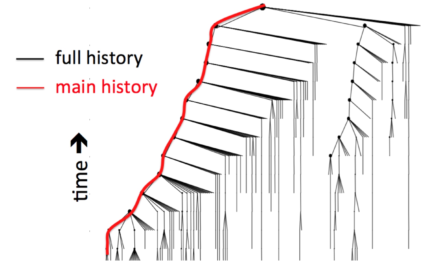
Figure 1: Two types of histories, main (red line) and full (all lines) for a single galaxy (the dot at the top). Dots are galaxies and lines connect them between time steps. Time flows upward. For the galaxy at the top (final time), the full star formation rate at any time is the sum of star formation rates of all dots (galaxies/halos) at the height corresponding to that time. All galaxies in the picture contribute to the full star formation rate. The main star formation rate history only includes the star formation rate of the single galaxy on the main (most massive progenitor) history of the galaxy, connected by the red line over time. A galaxy’s spectrum encodes the full star formation rate history (after dropping the contributions from stars which have been stripped, and including ageing). The main history is the star formation rate of what might be considered as a single galaxy evolving through time. Merger tree courtesy M. White.

Sample	method	range	$N_{\rm gal}$	all final galaxies above	history type
$M_{h}$	20 bins of $\leq 2000$	$10.60<\log M_{h}/M_{\odot}<15.60$	31383	$\log M_{h}/M_{\odot}>14.30$	main, full
	in $\log M_{h}$
$M^{*}$	20 bins of $\leq 2000$	$8.00<\log M^{*}/M_{\odot}<12.43$	34246	$\log M^{*}/M_{\odot}>11.77$	main, full
	in $\log M^{*}$
ran	random	$M^{*}/M_{\odot}>10^{9}$	32775	N/A	main, full
cen $M_{h,{\rm big}}$	all central galaxies	$M_{h}/M_{\odot}\geq 10^{12}$	386919	central $M_{h}/M_{\odot}\geq 10^{12}$	main

Table 1: Seven galaxy samples used for measurements. In the binned samples chosen from equally spaced logarithmic bins (final $M^{*}$ or $M_{h}$), 2000 galaxies were randomly chosen in each bin. However, in the highest bins, fewer than 2000 galaxies exist in the simulation; all galaxies were included above the scales as noted. Here, $M^{*}$, $M_{h}$ refer to values at final time.

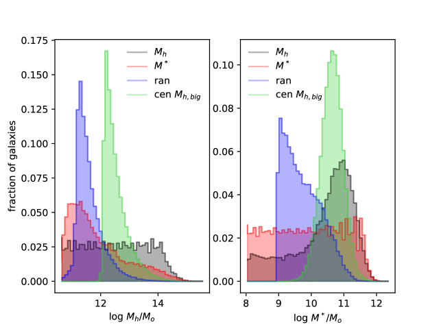
Figure 2: Final time halo mass and stellar mass distributions for the 4 simulation samples described in the text and Table 1. The $M_{h}$, $M^{*}$ and ran samples are all randomly selected according to some criteria, while the cen $M_{h,{\rm big}}$ sample includes all galaxies $M_{h}\geq 10^{12}M_{\odot}$ which are central at the last two time outputs.

There are two natural definitions of star formation rate histories, schematically illustrated with a sample simulated galaxy dark matter history in Fig. 1. All dark matter halos which eventually merge to form the final galaxy are shown. Time runs up the picture, with the single final galaxy at top, and progenitors appearing at the time when they are first resolved in the simulation (the size of dot is proportional to dark matter halo mass). The progenitors of the final galaxy that exist at any given time are shown on the same row, with lines connecting them to their descendants in the row above.

The full star formation rate history specifies the formation time of all stars in all galaxies which eventually merge to produce the final galaxy. At any give time, this rate is the sum of star formation rates across the appropriate row in Fig. 1. The full star formation rate history is encoded in the spectrum of the final galaxy, measured observationally, although stellar ageing and stripping can remove stars. Every star in the final galaxy was formed as part of the full star formation rate.

In contrast, the main star formation rate history is composed of the star formation rate of the largest progenitor galaxy at any time (here shown at left, with its history traced by the red line). The main star formation history considers the final galaxy as a single object throughout its history, with other galaxies merging into it. Such a galaxy could then be described, for instance, as moving through the blue cloud in a certain way, and onto the red sequence (if it quenches). Stars due to mergers did not form in the main history and thus are not related to this (“in situ”) star formation rate.

The full star formation rate history was considered by Diemer et al (2017) in the Illustris simulation, and by Pacifici et al (2016), who used spectra to get the star formation rate histories, and then matched them to a semi-analytic post treatment of the Millennium simulation histories. Both definitions of star formation rate histories are considered below.

2.1 Galaxy history samples

In order to study properties of galaxy histories as a function of halo mass or stellar mass, four galaxy samples are considered from the $\sim$ 2.26$\times 10^{7}$ galaxies at the scale factor $a=0.9997$ time step of the simulation (called the final time hereon). One sample is a random selection of galaxies with final $M^{*}>10^{9}M_{\odot}$. This sample is dominated by the lowest mass galaxies in the sample, due to the shape of the mass function. To better identify properties as a function of final halo or stellar mass, rather than being swamped by properties of low mass galaxies, random samples with a roughly uniform distribution in log final $M_{h}$ or log final $M^{*}$ were also created. All three subsamples have approximately 33000 galaxies, and full and main histories are studied for both. A fourth sample was taken for comparison with machine learning work by Kamdar, Turk & Brunner (2016a), and includes all galaxies with final time halo mass above $10^{12}M_{\odot}$ which are central at both the last and second to last time step (17% were satellites at some point in their histories). There are 386919 galaxies in this sample, so only the main star formation rate history was considered. These samples are called $M_{h}$, $M^{*}$, ran, and cen $M_{h,{\rm big}}$ below (with main or full to identify the choice of star formation rate history, except for cen $M_{h,{\rm big}}$ where only the main history was extracted). More details are in Table 1, and the stellar mass and halo mass distributions at final times are in Fig. 2. Besides highlighting higher $M_{h}$ and $M^{*}$ galaxies, using several subsamples illustrates how the fits below can be used to compare different galaxy samples (or different models built on the same or different simulations).

The starting redshift is 9.7 (when the universe is about 450 Myr old), and following Diemer et al (2017), star formation rate histories are integrated to the present day, using the galaxy formation model star formation rates at each output time. The integrated star formation rate from the initial time to time $t$ is $\tilde{\cal S}(t)$. For the seven samples here, there are 48 output times, outputs 11 to 58 in the MRscPlanck1 simulation.

Note that the final time integrated star formation rate $\tilde{\cal S}(t_{f})$ is not the final stellar mass. For the main histories, stellar mass gain due to mergers and stripping is not included. Although the full histories include all stars formed by galaxies which eventually merge into the final galaxy, they still do not account for stars which are stripped off, or those which are added by stripping of other galaxies which don’t eventually merge, and again, for both, starbursts are not available at the simulation output times. In both cases, the stars age as well.

These integrated histories $\tilde{\cal S}(t)$ are assigned peak times, using a lognormal fit (following Gladders et al (2013); Diemer et al (2017)) and principal component expansions around the average history as follows.

2.2 Lognormal fit

For the lognormal parameterization, star formation rate (SFR) histories are taken to have the form (Diemer et al, 2017),

$$SFR_{\rm log}(t)=\frac{A}{\sqrt{2\pi}\tau t}\exp(-\frac{(\ln t-T_{o})^{2}}{2\tau^{2}}),$$ (1)

with corresponding integrated star formation rate history

$$\begin{array}[]{ll}\tilde{\cal S}_{\rm log}(t)&=\frac{A}{2}\{1-{\rm erf}(-\frac{\ln t-T_{0}}{\tau\sqrt{2}})\}\\ &=\int_{t_{\rm initial}}^{t}SFR_{\rm log}(t^{\prime})dt^{\prime}\;.\\ \end{array}$$ (2)

Fits are done to this integrated star formation rate history, following Diemer et al (2017), due to its reduced scatter.

This parameterization has a peak time, width and peak SFR

$$\begin{array}[]{lll}t_{\rm peak}&=&e^{T_{0}-\tau^{2}}\\ \sigma_{t}&=&2t_{\rm peak}\sinh(\sqrt{2\ln(2)}\tau)\\ SFR_{\rm peak}&=&\frac{A}{\sqrt{2\pi}\tau}e^{-T_{0}+\tau^{2}/2}\end{array}$$ (3)

The width $\sigma_{t}$ is the amount of time between the two points in the history where the star formation rate is above $1/2$ of its peak value. More generally (Diemer et al, 2017), the time where the star formation rate reaches $1/\beta$ of its peak value, $SFR(t_{\beta})=\frac{1}{\beta}SFR_{\rm peak}$ is

$$t_{\pm 1/\beta}=t_{\rm peak}e^{\pm\tau\sqrt{2\ln(\beta)}}\;.$$ (4)

One particular value of interest is $t_{1/2}$, where the star formation rate drops to half of its peak value (it is part of $\sigma_{t}=t_{1/2}-t_{-1/2}$ and can be roughly thought of as a sort of quenching parameter).

Diemer et al (2017) applied this lognormal fit to integrated star formation rate histories in the Illustris simulation, as well to the integral of observed average quiescent galaxy star formation rate histories stacked by Pacifici et al (2016), and compared to similar fits on observations by Gladders et al (2013). They used the 29203 galaxies in Illustris with $M^{*}\geq 10^{9}M_{\odot}$, integrating the star formation rates starting when the universe was 54 Myr old along 100 equally spaced output times.

For Illustris, the parameters $t_{\rm peak},\sigma_{t}$ are correlated, obeying a mean relation,

$$\sigma_{t}\sim 0.83t_{\rm peak}^{3/2}\;{\rm in\;Gyr}.$$ (5)

(For example, see Figs. 5 and 6 in Diemer et al (2017).)

By construction, this fit is an approximation. They defined the goodness of fit for their parameterization as

$$D={\rm max}_{t}\frac{|\tilde{\cal S}_{\rm log}(t)-\tilde{\cal S}(t)|}{{\rm max}(\tilde{\cal S}(t))}\;.$$ (6)

and found that satellites tended to have worse fits than central galaxies. This goodness of fit measure will be used below for both approximations and all 7 samples.

2.3 Principal component analysis

Principal component analysis (PCA) offers another approximation to galaxy integrated star formation rate histories. For PCA in general, vectors are decomposed into the average of the sample, plus coefficients $a_{n}$ times principal components $PC_{n}$. The $PC_{n}$, basis vectors for fluctuations around the average, are eigenvectors of the covariance matrix of the vector components. The integrated star formation rate history of one galaxy up to a particular time is an element of the vector $\tilde{\cal S}(t)$ for that particular galaxy. The full ensemble of a sample’s integrated star formation rate histories, for all of its galaxies, determines the average and the fluctuation vectors $PC_{n}(t)$.

In more detail, the integrated star formation rate histories are first normalized by dividing the integrated star formation rate histories by each galaxy’s individual integrated star formation rates at the final time,

$${\cal S}(t)=\tilde{\cal S}(t)/\tilde{\cal S}(t_{f})\;.$$ (7)

(Again, as mentioned earlier, $\tilde{\cal S}(t_{f})$ is not necessarily the same as final $M^{*}$.) Without this normalization, the sample average and fluctuations around it are dominated by the most massive galaxies, as these tend to have the largest integrated star formation rates and fluctuations. Other candidates for rescaling $\tilde{\cal S}(t)$, using the final stellar mass or the peak star formation rate, gave much larger scatters around the resulting average history.

The vector ${\cal S}^{\alpha}(t)$, the normalized integrated star formation rate history of any galaxy labeled by $\alpha$, is then written using PCA as

$${\cal S}^{\alpha}(t)=\bar{\cal S}(t)+\sum_{n=0}^{N_{\rm times}-1}a_{n}^{\alpha}PC_{n}(t)\;.$$ (8)

with constant coefficients $a_{n}^{\alpha}$. Here the average $\bar{\cal S}(t)=\frac{1}{N_{\rm gal}}\sum_{\alpha}{\cal S}^{\alpha}(t)$. The PCA basis fluctuations $PC_{n}(t)$ are the orthonormalized eigenvectors of the covariance matrix, $C_{ij}=\langle{\cal S}(t_{i}){\cal S}(t_{j})\rangle$. There are as many fluctuation basis vectors $PC_{n}(t)$ as there are output times $t_{i}$, 48 for the samples under study here, and the expression Eq. 8 is exact. The largest contribution to the sample variance is in the direction $PC_{0}(t)$, followed by $PC_{1}(t)$, etc. (For parameter counting, to give the unnormalized history there is one additional parameter, to undo the rescaling which made ${\cal S}(t_{f})\equiv 1$ for each galaxy. Because of this constraint, the variance in the direction of $PC_{47}(t)$, a vector of zeros except for a 1 at final time, is 0.)

An approximation to the integrated star formation rate history can be made by truncating the expansion Eq. 8, keeping only some of the $PC_{n}(t)$. Hereon, the PCA approximation is taken to be the truncation of the above expansion to the first three components:

$${\cal S}^{\alpha}(t)\approx\bar{\cal S}(t)+a_{0}^{\alpha}PC_{0}(t)+a_{1}^{\alpha}PC_{1}(t)+a_{2}^{\alpha}PC_{2}(t)\;.$$ (9)

If this approximate description of average history plus a few fluctuations is to be useful, a large fraction of the variance of the sample should be captured using the first few basis fluctuations, that is, by the sum of the first few eigenvalues of the covariance matrix. Not unrelated, but not automatic, for the approximation to be good for any particular galaxy labeled by $\alpha$, the $a_{n}^{\alpha}$, for $n>2$, should be relatively small, for example, in comparison to the variance around the average for the full sample. Again, in the PCA decomposition, both the $PC_{n}(t)$ and the average integrated history, $\bar{\cal S}(t)$, are properties of the sample, and depend upon the galaxy histories used. The sample depends upon its selection function, and the galaxy histories of course depend upon the theory used to construct them.

3 Parameterizing galaxy histories

The lognormal fit, Eq. 3, and PCA approximation, Eq. 9, were implemented for all seven galaxy samples in Table 1. Some properties of the fits, in particular, the values of the leading parameters, $t_{\rm peak}$ and $a_{0}$, their relation, and measures of goodness of the fits, are as follows.

3.1 Lognormal Fit

The distribution of $t_{\rm peak}$, is shown at top in Fig. 3 for all 7 samples. It is weighted towards early times, especially in the $M^{*}$ and $M_{h}$ samples, which have the largest fraction of massive and thus early forming galaxies.

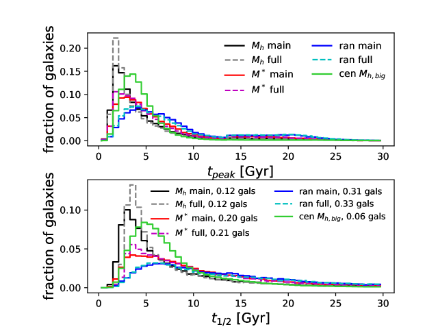
Figure 3: Distribution of (top) peak time $t_{\rm peak}$ and (bottom) $t_{1/2}$ for integrated star formation rate histories for all 7 samples, from their fits to a lognormal as in Eq. 2. The time $t_{1/2}$ is calculated from the lognormal fit and corresponds to the time in the fit when galaxies drop to 1/2 of their peak star formation rate. The legend also shows the fraction of galaxies with $t_{1/2}>30$ Gyr, i.e. those dropping to half of their peak star formation rate after 30 Gyr. Although $t_{1/2}$ is related to the quenching time, it is not exactly when the galaxy leaves the star forming main sequence, as the latter also depends upon stellar mass and redshift. The main samples are shown with a solid line, the full samples are shown with a dashed line of similar color.

Another characteristic time, as mentioned above, is when a galaxy drops to 1/2 of its peak star formation rate, $t_{1/2}$, shown at the bottom of Fig. 3. Although related to quenching, $t_{1/2}$ does not specify on its own when a galaxy leaves the star forming main sequence, as the star forming main sequence changes with redshift and depends on the stellar mass of the galaxy (see, Speagle et al (2014), for example, for different estimates of where the star forming main sequence lies, depending upon definitions of stellar mass and star formation rates).

Galaxy by galaxy, on average, the full samples have slightly earlier $t_{\rm peak}$ (0.12-0.25 Gyr) and larger $\sigma_{t}$ (0.74-1.35 Gyr). That is, the time evolution of the combined star formation rate of all the progenitor galaxies of a final galaxy on average peaks earlier but decays more slowly than that for the single main galaxy. This effect has many contributing factors which would be interesting to better understand, including the smaller mass of the galaxies which merge onto the main galaxy, their tendency to quench when they fall into the main galaxy’s halo, and the relation of the merger rate to the star formation rate of the main galaxy.

For these samples, the $t_{\rm peak}-\log\sigma_{t}$ correlation is about 80% and the two parameters obey a similar mean relation to that of Illustris, where $\sigma_{t}\sim 0.83t_{\rm peak}^{3/2}$ (Diemer et al, 2017). In the cases here, the power law remains close to 1.5 , but the prefactor varies by a factor of two between samples with different mass distributions. The full ran sample, expected to have sampling closest to the Illustris distribution, obeys $\sigma_{t}\sim 0.68t_{\rm peak}^{1.62}$. Bluck et al (2016) compared both models to observations and found that L-galaxies (Henriques et al, 2015) quench too quickly and Illustris galaxies not quickly enough, consistent with Illustris having a larger $\sigma_{t}$ for a given $t_{\rm peak}$ as found here.

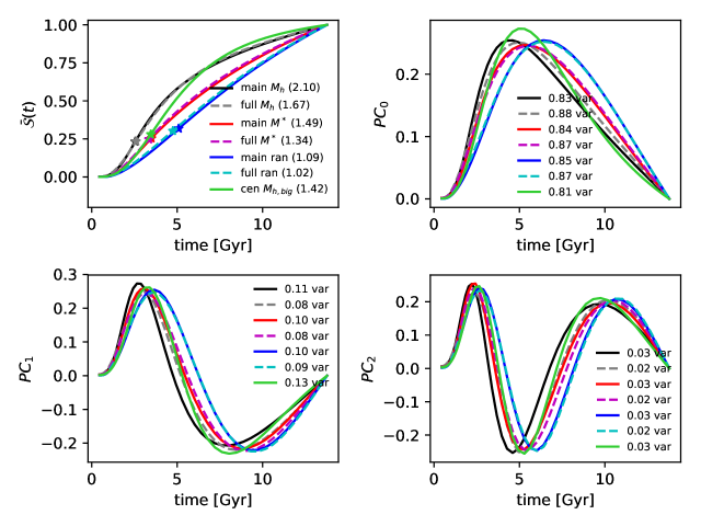
Figure 4: Basis PCA components for the expansion of galaxy histories (each normalized to 1 at final time). Individual galaxy histories are approximated via ${\cal S}(t)\approx{\cal\bar{S}}(t)$ + $a_{0}PC_{0}(t)+a_{1}PC_{1}(t)+a_{2}PC_{2}(t)$, Eq. 9. Upper left: the average history $\bar{\cal S}(t)$ for all 7 samples, labelled with total variance for each. Stars mark the lognormal fit $t_{\rm peak}$ for each average. The earliest $t_{\rm peak}$ occurs for the samples with the largest number of massive galaxies. The leading three fluctuations around each average are $PC_{0}(t)$ at upper right, $PC_{1}(t)$ at lower left, and $PC_{2}(t)$ at lower right, labeled with the fractional contribution of each $PC_{n}$’s coefficients to the total variance. For each $n$, the $PC_{n}(t)$ show ordering in their features similar to the $t_{\rm peak}$ in their sample averages. The full and main averages essentially coincide for all samples. The full and main $PC_{n}(t)$ all coincide for the ran sample, but differ in $PC_{0}(t),PC_{1}(t)$ for the $M_{h}$ sample, and $PC_{1}(t),PC_{2}(t)$ in the $M^{*}$ sample.

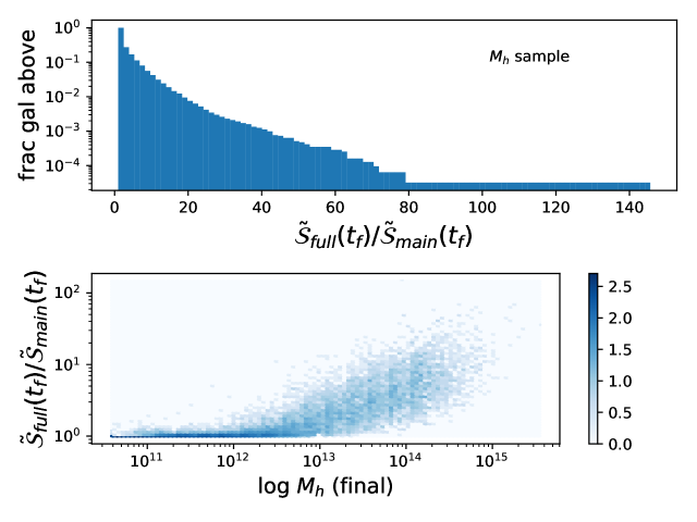
Figure 5: Top: fraction of galaxies with given ratios of full to main final integrated star formation rates, $\tilde{\cal S}_{\rm full}(t_{f})/\tilde{\cal S}_{\rm main}(t_{f})$. After dividing by these normalizations, the full and main average integrated histories almost coincide, see upper left in Fig. 4.
Bottom: Final $M_{h}$ dependence of $\tilde{\cal S}_{\rm full}(t_{f})/\tilde{\cal S}_{\rm main}(t_{f})$, $\log_{10}$ number of galaxies in each pixel according to scale at right.

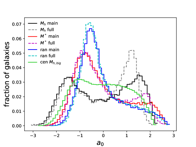
Figure 6: Distribution of $a_{0}$ for all 7 samples. As $a_{0}$ is the coefficient of $PC_{0}(t)$ (shown in Fig. 4, upper right), positive $a_{0}$ increases the integrated star formation rate at early times relative to the average, and negative $a_{0}$ decreases it, corresponding to later star formation. Full and main distributions separate at positive $a_{0}$ for samples with many large final $M_{h}$ galaxies. For these, main histories tend to have a larger positive $a_{0}$, i.e., an earlier rise in integrated star formation rate. The variance in this coefficient captures (depending on sample) from 81% to 88 % of the total variance around the average, as noted in Fig. 4.

3.2 Principal Component Analysis

Turning to principal analysis, the average histories $\bar{\cal S}(t)$ and leading three fluctuations, $PC_{0}(t),PC_{1}(t),PC_{2}(t)$ are shown in Fig. 4 for all 7 samples. The average history $\bar{\cal S}(t)$ is at upper left. The total variance around each $\bar{\cal S}(t)$ is listed in the legend and a star marks the lognormal fit $t_{\rm peak}({\bar{\cal S}(t)})$ for each. The other panels show the first 3 principal components, and list their respective fractional contributions to the total variance for each sample. (Again, solid lines are main histories, dashed are full histories.) These first 3 fluctuations have $\geq 97\%$ of the total scatter around the average. This is a better approximation than that found by applying PCA to the star formation rate histories themselves. In the latter case, again rescaling by $\tilde{\cal S}(t_{f})$, all samples except cen $M_{h,{\rm big}}$ require $>10\;PC_{n}$ to capture 90% or more of the variance around the average history. (The cen $M_{h,{\rm big}}$ sample requires 6 $PC_{n}$.) The smaller fraction of variance in the first 3 fluctuations around the instantaneous star formation rate makes the PCA approximation, Eq. 9, much less useful.

Comparing samples, as the number of lower $M^{*}$ galaxies (which tend to be star forming) increases, there is a trend towards later sample average $t_{\rm peak}$ and correspondingly later times for the peaks of the principal components. This is in line with the tendency of lower $M^{*}$ galaxies to quench at later times. The average histories of each of the subsamples seem independent of whether the full or main histories are used. This is in spite of very different full to main normalizations, a comparison of $\tilde{\cal S}_{\rm full}(t_{f})$ and $\tilde{\cal S}_{\rm main}(t_{f})$ is in Fig. 5 for the $M_{h}$ sample. The bottom panel shows their ratio as a function of final $M_{h}$ (the trend with final $M^{*}$ was weaker). Higher $M_{h}$ halos have larger ratios of full to main ${\tilde{\cal S}}(t_{f})$, that is, they have more star formation in their full history which was not “in situ”, i.e., not in the main star formation rate history.

Most of the variance around the average history is captured in the coefficient of the leading fluctuation $PC_{0}(t)$, $a_{0}$. Fig. 6 shows the distribution of $a_{0}$ for all 7 samples. From Fig. 4, it can be seen that adding $PC_{0}(t)$ to the average history with a positive coefficient $a_{0}$ will cause the integrated star formation rate to rise earlier than the average history, and a negative $a_{0}$ will cause a later rise in the integrated star formation rate history. Although the full and main average histories (and $PC_{0}(t)$, except for the $M_{h}$ sample) closely overlap, the positive $a_{0}$ distributions strongly different between the full and main histories for the $M_{h},M^{*}$ samples, which have a large number of high mass halos. (The full cen $M_{h,{\rm big}}$ sample was not downloaded, as mentioned earlier.)

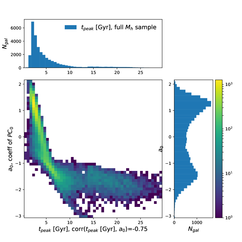
Figure 7: Comparison of lognormal and PCA approximations via their leading parameters $t_{\rm peak}$ and $a_{0}$. Top: the $t_{\rm peak}$ distribution for the full $M_{h}$ sample. Far right: the $a_{0}$ distribution. Bottom left: the logarithm of the number of galaxies sharing each pair of values. Although a correlation is visible, the relation between $t_{\rm peak}$ and $a_{0}$ changes noticeably for low $a_{0}$ and large $t_{\rm peak}>7$ Gyr, i.e. for galaxies which have star formation at later times. Even with this flat tail, there is a high $a_{0},t_{\rm peak}$ correlation of galaxies shown (the highest $t_{\rm peak}>30$ Gyr objects are dropped, about 0.1% of this sample). These trends in the joint distribution of are seen in all samples; correlations range from -0.70 to -0.75, again using galaxies with $t_{\rm peak}<30$ Gyr (up to 0.4% of galaxies in the ran sample). Similar correlations are found with $t_{1/2}$.

3.3 Comparison of lognormal and PCA approximations

3.3.1 Relation of leading parameters

The two parameterizations are related. In particular, the PCA leading contribution, $a_{0}$, is correlated with the lognormal fit parameter $t_{\rm peak}$. Their relation is shown for the full $M_{h}$ sample in Fig. 7. Roughly, a late $t_{\rm peak}$ corresponds to a negative $a_{0}$, meaning the rise in the integrated star formation rate occurs at a later time. The correlation is similarly strong for $a_{0}$ with $\ln\sigma_{t}$, expected given the mean relation for $\sigma_{t}(t_{\rm peak})$, and with $t_{1/2}$, the time when star formation rate in the fit falls to half of its maximum. Relations for the other 6 samples are comparable in shape and size. The relation between the two parameters visibly changes for larger $t_{\rm peak}\gtrsim 5$ Gyr, presumably because the shape of $PC_{0}(t)$ is not flexible enough to approximate star formation rates peaking at late times, see below. In addition, the integrated histories for galaxies with later $t_{\rm peak}$ tend to be very close to each other (more elaboration in §5 below).

In spite of the many correlations, the fits have key differences. In particular, $t_{\rm peak}$ for each galaxy is independent of the full galaxy sample used, defined solely in terms of fitting to a predetermined lognormal shape. In contrast, $a_{0}$ depends upon the full sample (which determines both $PC_{0}(t)$ and the average) but has no prior assumptions about the shape of the histories. Also, for the $t_{\rm peak}$ parameterization, for different galaxies the peak moves in position and changes in width (the integral of the height is fixed). In the PCA approximation, varying the PCA coefficients can alter the sign and amplitude of each of the fluctuations $PC_{n}(t)$ around the fixed average, but not their shape. The $t_{\rm peak}$ parameterization enforces that the integrated star formation rate is monotonic, while the approximation using the first 3 $PC_{n}(t)$ does not require this (as mentioned earlier, its derivative can thus lead to negative instantaneous star formation rates, these unphysical star formation rates are set to zero).

3.3.2 Approximating histories

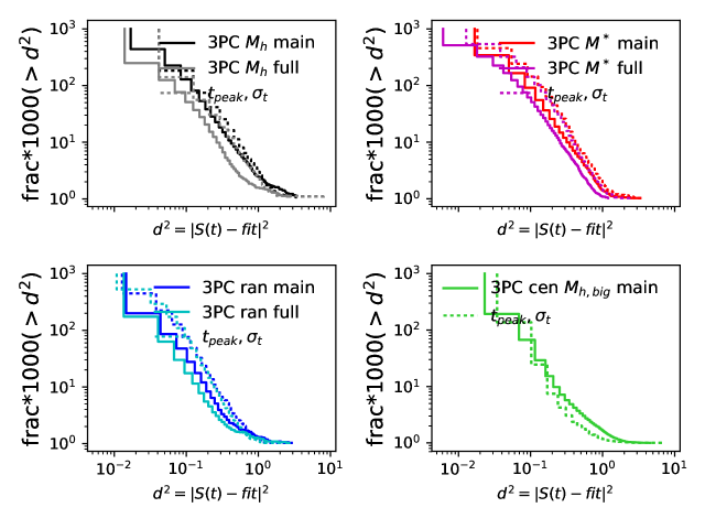
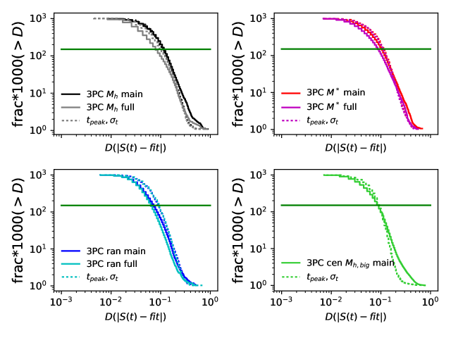
Figure 8: Accuracy of approximating normalized integrated histories ${\cal S}(t)$ by first three PCA coefficients $a_{0},a_{1},a_{2}$ (solid line) or by 2 parameters of the lognormal fit, e.g.,$t_{\rm peak},\sigma_{t}$ (dotted line). Top: the cumulative fraction of galaxies with a square of the separation between the approximate and simulated ${\cal S}(t)$ above a given value, times 1000. Bottom: 1000 times the cumulative number of galaxies above a separation measure $D$, defined in Eq. 6, along with a line marking 15% of the galaxies. In Diemer et al (2017), for Illustris, the 15% line crosses the distribution at a lower $D$, $D=0.05$. In both, the best fits are for the ran samples.

Two measures of the goodness of fit to ${\cal S}(t)$, the squared “distance” $d^{2}=|fit-{\cal S}(t)|^{2}$ and the goodness of fit criterion $D$ in Eq. 6, roughly the maximum spacing between the history and the fit, are shown in Fig. 8. Solid lines are the PCA approximation, dependent upon $a_{0},a_{1},a_{2}$, and dashed lines are the lognormal fit, dependent upon $t_{\rm peak}$ and $\sigma_{t}$. (As ${\cal S}(t)$ is used here, the parameters $\tilde{\cal S}(t_{f})$ and $A$ drop out. Scaling out these factors is automatic in $D$, and for $d^{2}$ it prevents the high mass galaxies from swamping the signals as well as making intercomparisons more difficult. ) The two methods give roughly the same quality of fit by these measures, sample by sample. The ran samples have the best fits. Relative to the other samples, the ran samples also have more satellites (noted to have worse lognormal fits in Diemer et al (2017)), but fewer high mass halos. The $d^{2}$ for the two approximations are correlated, good or bad fits tend to occur together. Many of the $D>0.05$ fits can be seen by eye to be due to rejuvenating histories, where two bouts of star formation occur, separated by a period of quiescence. Diemer et al (2017) found 15 % of the Illustris galaxies had $D>0.05$, the 15% line horizontal crosses each sample’s distribution in Fig. 8 at larger values, that is, the fits are worse for these samples than for Illustris.

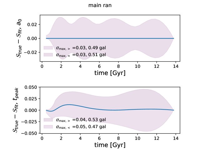
Figure 9: Average difference of the approximations and the true (simulation) normalized histories $\langle{\cal S}_{\rm true}(t)-{\cal S}_{\rm fit}(t)\rangle$ and scatter, as a function of history time step. The top panel corresponds to the PCA approximation, and the bottom panel to the lognormal approximation, in the main ran sample. The shaded regions are one standard deviation, calculated separately for galaxies with ${\cal S}_{\rm true}(t)-{\cal S}_{\rm fit}(t)$ above or below the average. The total fractions of galaxies above and below the average, over all 48 time steps, are given by the numbers shown, as well the maximum standard deviation (“var max”) in each direction. See text for more discussion.

To get a sense of how the histories deviate from their fits in more detail, the average of ${\cal S}_{\rm true}(t)-{\cal S}_{\rm fit}(t)$ is shown for the main ran sample in Fig. 9. The full ran sample is similar. This average is zero for the PCA approximation by construction, but slightly nonzero for the lognormal fit. The shaded regions are the standard deviations (calculated for top and bottom separately) for each time step. These are up to 5% of the final value (which is 1) for this sample. The PCA approximation error is the sum of the neglected principal components in Eq. 8, its standard deviation generally has an oscillatory envelope, and the envelope is $\leq 0.05$ across samples, compared to $\leq 0.07$ for the lognormal fit (and in every sample the deviation for PCA was $\leq$ that for the lognormal - 0.02).

3.3.3 Approximating final time star formation rate

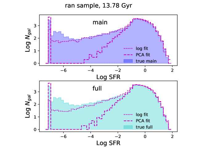
Figure 10: Final time SFR distribution in the main (top) and full (bottom) ran samples. The true (simulation) values are given by the shaded histogram. Galaxies with SFR $<10^{-7}M_{\odot}yr^{-1}$ are assigned SFR $10^{-7}M_{\odot}yr^{-1}$. Dots show the lognormal fit and dashed show the PCA fit. Starting at the highest star formation rates, the number of galaxies rises as the star formation rate decreases, and then flattens out, eventually decreasing more, and ending with a peak at the minimum star formation rate. The other samples, with more high mass halos, have worse fits at higher star formation rates. For these, again starting with the highest star formation rates, the number of galaxies tends to continue to increase beyond (below) star formation rates where the simulation number of galaxies flattens, giving an excess.

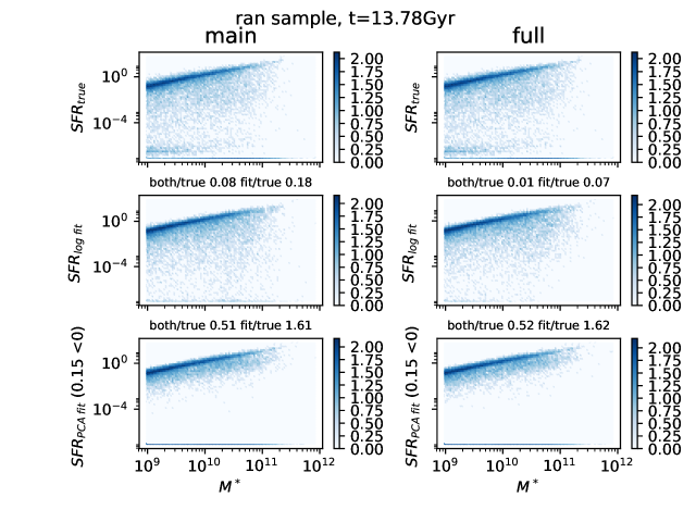
Figure 11: Stellar mass (in units of $M_{\odot}$) vs. star formation rate (in units of $M_{\odot}$ yr^-1) at final time in the simulation (top panel, same at left and right), as compared to the lognormal (middle) and PCA (bottom) approximations. Main histories are at left, to the full histories at right. The star forming main sequence is visible at top ($\log N_{\rm gal}$ per pixel shown in the bars at right). Galaxies with $SFR<10^{-7}M_{\odot}yr^{-1}$ are assigned the minimum $SFR=10^{-7}M_{\odot}yr^{-1}$, including the 15% of PCA fit galaxies with $SFR<0$ in this sample. The “green valley” between the minimum $SFR$ and the star forming main sequence has fewer galaxies in the PCA fit, compared to the lognormal fit or simulation. “both”, “true”, and “fit” refer to the number of galaxies with minimum SFR common to the simulation and fit, in the simulation, or in the fit, respectively, with ratios as shown. Relative to the simulation, in the ran sample more galaxies are quiescent in the PCA fit (fit/true $>1$) and fewer are quiescent in the lognormal fit (fit/true $\ll$ 1); these numbers vary with sample.

One can also step back and compare the fits to the histories to the simulation at a fixed time, for instance at $z=0$. The final star formation rate distribution is shown in Fig. 10 for the ran sample. The shaded region is the final time star formation rate distribution of the simulation, identical for the main (top) and full (bottom) samples. Any rates $<10^{-7}M_{\odot}yr^{-1}$, including possible negative ones from the PCA construction, are set to $10^{-7}M_{\odot}yr^{-1}$. The lognormal fit has many more galaxies in the green valley, closer to the shape of the star formation rate distribution in the simulation. In contrast, there are more galaxies with the minimum star formation rate in the PCA fits; their number then drops precipitously in the green valley. Adding more principal components can increase the number of galaxies lying in the green valley, but even using 38 components, i.e. including up to $a_{37}PC_{37}$, did not reach the approximate agreement at final time in the green valley found by using the lognormal fits. In the other samples, with more high mass galaxies, the agreement between the fit at higher star formation rates is worse. An excess appears for these other samples at the higher star formation rates, which persists to lower star formation rates for the lognormal fit.

There is slightly different information in the instantaneous stellar mass-star formation rate diagram, with the star formation rates again calculated from the fits to the integrated histories. This relation is shown in Fig. 11. The top two panels are the simulation, which is identical on the left and right, again because this is the final time. Below are the final time star formation rates based upon fits to the the main (left) and full (right) integrated star formation rate histories. The middle panel is the lognormal fit, the bottom panel the fit from PCA. (The fraction of galaxies with negative rates in the PCA fit is listed on the y-axis for the lower 2 panels.) In the simulation and both fits, a star forming main sequence is evident, but in the PCA fit, the absence of galaxies in the “green valley” between star forming and quiescent is again noticeable. The numbers of galaxies with the minimum star formation rate $\leq 10^{-7}M_{\odot}yr^{-1}$ are compared in the simulation and the fits. Those which are common to both the fit and the simulation (“both”), and those present in the fit (“fit”) are divided by the number in the simulation (“true”). The lognormal fit lacks some of these quiescent galaxies, while the PCA fit has too many, relative to the simulation. For other samples,“fit/true”$<1$ for all of the lognormal fits, and for the $M_{h}$ and cen $M_{h,{\rm big}}$ PCA fits.

To summarize, the galaxy histories were approximated with two fits. The lognormal description assigns each history a peak, which can move in time, and a width of lognormal shape, while the PCA approximation treats all histories in a sample as the sum of the same average history plus perturbations with fixed position and shape, derived from the sample, with the perturbation coefficients changing for different galaxies. The PCA approximation, which normalizes the integrated star formation rate histories before expanding them, has similar averages and basis fluctuations for the full and main histories. The PCA normalization factors, i.e., the final integrated star formation rates, differ the most between full and main histories for galaxies with higher final $M_{h}$. In the lognormal fit, the peak time is slightly earlier for the full samples, and the width slightly larger. The lognormal and PCA approximations have correlated leading parameters and give similar “distances” (as shown in Fig. 8) from the simulated histories, using two estimates of goodness of fit.

One use of these fits is to compare their parameters to final time galaxy properties and histories of other galaxy properties, explored next.

4 Galaxy star formation rate fits compared to other galaxy properties

With the parameterizations based upon a lognormal fit or PCA in hand, their relation to other galaxy properties can be explored, such as the observable final time $M^{*}$ and $SFR$, the in principle observable final time $M_{h}$, and properties of main histories for halo mass and stellar mass. Recall that the full (rather than main) histories of galaxy halos and other dark matter properties are combined with the full semi-analytic model to create the detailed star formation rate histories in the first place. Both correlations and machine learning can be used to analyze these relations.

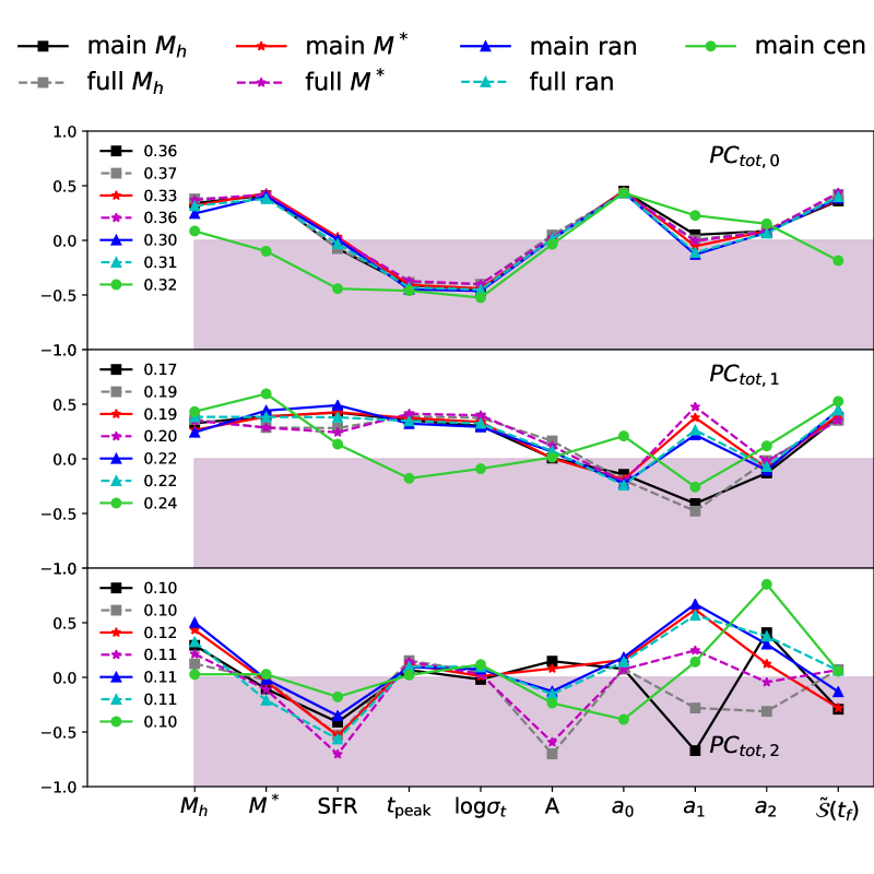
Figure 12: First 3 principal components for joint changes in final $M_{h}$, final $M^{*}$, final SFR, lognormal fit parameters $t_{\rm peak}$, $\log\sigma_{t}$, $A$, and PCA fit parameters $a_{0}$, $a_{1}$,$a_{2}$, $\tilde{\cal S}(t_{f})$. These three vectors are the combinations of variations which dominate the normalized scatter of the 10$\times$ 10 correlation matrix of each sample. The fraction of the scatter in each $PC_{{\rm tot},n}(t)$ is shown at left, for each sample. The shading shows where zero correlation lies. The leading contribution to the scatters, $PC_{{\rm tot},0}(t)$, shows that final $M^{*}$, final $M_{h}$ and $a_{0}$ tend to fluctuate opposite to $t_{\rm peak},\sigma_{t}$. The subleading contributions show $a_{1}$ as related to final $M_{h}$, final $M^{*}$, and, in the next leading combination, having sample dependent relations. The different samples have different fractions of high final $M_{h}$ or $M^{*}$ galaxies, Fig. 2.

4.1 Correlations

Because there are correlations between galaxy histories and galaxy final properties, for example, more massive galaxy halos tend to have galaxies which quenched earlier, correlations are expected between $a_{0}$, $t_{\rm peak}$ and final time $M_{h},M^{*}$ and $SFR$. The halo mass $M_{h}$ refers to the host (sub)halo of a galaxy (“mvir” in the Millennium simulation, i.e., its $M_{200c}$ mass when it was last a central galaxy).

Quantities which are expected to be related to each other include final $M_{h}$, final $M^{*}$, final SFR, and parameters from both fits: $t_{\rm peak}$, $\log\sigma_{t}$, $A$, $a_{0},a_{1},a_{2}$ and $\tilde{\cal S}(t_{f})$. Although the $a_{i}$ are uncorrelated with each other by construction, the rest of the parameters tend to be correlated with each other (e.g. the $\sigma_{t}(t_{\rm peak})$ relation, or the $M^{*}(M_{h})$ relation in the final time observables). The list of cross correlations between all 10 components, for 7 samples, is unwieldy. Here, to get some idea of how variations are related, the combinations of the correlations between all of these quantities which dominate the (normalized) scatter are found, i.e., PCA, but for the correlation matrix. Correlations are used because of the wide ranges of the different quantities. Instead of the first 3 combinations of variations comprising $\geq$95% of the scatter, such as for the integrated star formation rate histories, here the first 3 combinations, shown in Fig. 12 capture $\sim$2/3 of the (normalized) scatter. However, the leading combinations do capture a large amount of scatter and can be used to look at trends. The fraction of (normalized) variance captured in each $PC_{{\rm tot},n}(t)$ is listed to the left for $PC_{{\rm tot},0}(t)$ (top), $PC_{{\rm tot},1}(t)$ (middle), and $PC_{{\rm tot},2}(t)$ (bottom) . For example, $PC_{{\rm tot},0}(t)$, with $\sim 1/3$ of the normalized scatter, has the parameters $t_{\rm peak},\sigma_{t}$ change in the same direction and by similar amounts (as expected due to their mean relation), and in opposition to $a_{0}$, with the expected relations to halo mass and stellar mass also visible. That is, high $M^{*}$ or high $M_{h}$ is associated with low $t_{\rm peak}$, which is the familiar relation of high stellar mass galaxies forming stars earlier. Differences between samples can be seen, which might in particular indicate some mass dependence (the $M_{h}$, $M^{*}$ samples have more high $M_{h}$ or $M^{*}$ galaxies, see Fig. 2).

There are also, of course, correlations of the integrated star formation rate parameters with the main $M_{h}$ or $M^{*}$ histories, as all these histories are related. There are several ways to compare the $M_{h}$ histories, $M_{h}(t)$, to the star formation rate history parameterizations. (The notation $M_{h}(t)$ refers to the main halo history, analogous to the main star formation rate history, i.e. the red line in Fig. 1.) For the lognormal fit, Diemer et al (2017) compared $t_{\rm peak},\sigma_{t}$ from the Illustris simulation with parameters for halo history fits of Wechsler et al (2002); Tasitsiomi et al (2004); McBride, Fakhouri & Ma (2009), using only the times the galaxies were in halos, rather than as satellites in subhalos. They found trends for $t_{\rm peak}$ with halo formation redshift $z_{\rm wechsler}$ for $t_{\rm peak}$, in 3 different stellar mass bins. (They noted their scaling $\sigma_{t}\sim 0.83t_{\rm peak}^{3/2}$ did not seem to arise naturally from the analytic (Dekel et al, 2013) mass accretion rate for a halo.) For the samples here, the correlation of $t_{\rm peak}$ with half mass redshift was highest for the samples with the latest average $t_{\rm peak}$, $\sim$ -50% for ran, dropping to magnitude $<10\%$ for the $M_{h}$ samples. Correlations were similar, with opposite sign, for $a_{0}$ and half mass redshift. Using PCA for $M_{h}(t)$, normalized to end at 1 (unlike the integrated star formation rate history, $M_{h}(t)$ does not have to be monotonic), correlations between $a_{0,h}$ and $a_{0}$ and $t_{\rm peak}$ were small (below 20%) for all samples except the ran samples, where they were $\sim\pm$30%.

A close relation is expected between the integrated star formation rate and the main stellar mass history, as $M^{*}(t)$ is the sum of stellar mass formed within the galaxy (the “main” integrated star formation rate) plus contributions from mergers, stripping by and of other galaxies, and ageing (instantaneously applied in the semi-analytic models). Correlations between $a_{0}$ and its stellar mass history counterpart $a_{0,*}$ are $\sim 76-97$%, with the random sample having the largest correlation (for samples with both main and full integrated star formation rate, both are similarly correlated with $a_{0,*}$). The fluctuation $PC_{0}$ in the integrated star formation rate is associated with more of the scatter than its counterpart in the stellar mass histories.

4.2 Halo mass at $t_{\rm peak}$: $M_{h,{\rm peak}}$

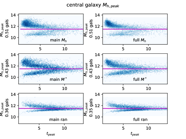
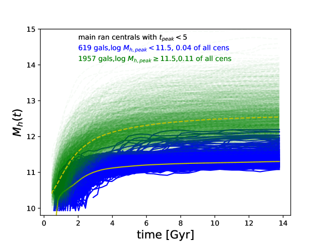
Figure 13: Top: central galaxy main halo mass $M_{h}$ at peak time $t_{\rm peak}$, $M_{h,{\rm peak}}$, as a function of $t_{\rm peak}$. The fraction of galaxies in each sample which are central at all times and have $t_{\rm peak}$ in the past is noted at left for each panel. Samples are as listed for $M_{h},M^{*}$ and ran, top to bottom, with main integrated star formation rate histories at left, full integrated star formation rate histories at right. The magenta horizontal line at $\log M_{h,{\rm peak}}/M_{\odot}=11.5$ divides these galaxies into two groups. For the majority of central galaxies, which are above the horizontal magneta line, $M_{h,{\rm peak}}$ seems to decrease with increasing $t_{\rm peak}$. Bottom: In blue, the halo histories for the 619 central galaxies (of 17278 total central galaxies) below the dividing line shown in panels above, i.e. with $M_{h,{\rm peak}}<10^{11.5}M_{\odot}$, and with $t_{\rm peak}<5$ Gyr. Unlike most other halo histories for galaxies with $t_{\rm peak}<5$Gyr, shown as green lines, the low $M_{h,{\rm peak}}$ galaxy halo masses seem to stall at low values. The averages of the two samples, including only nonzero histories at each step, are shown by the solid yellow and dashed yellow lines.

In the lognormal fit, another way of comparing the halo history to $t_{\rm peak}$ is to consider $M_{h}(t_{\rm peak})\equiv M_{h,{\rm peak}}$. This characteristic mass at peak star formation rate is shown in in Fig. 13 for all central galaxies in the $M_{h}$, $M^{*}$ and ran samples. This mass is only available for galaxies with $t_{\rm peak}$ in the past, and satellites are excluded because their $t_{\rm peak}$ is expected to also depend on their time of infall into a larger halo. Only galaxies which have been central at all times are counted as central.

In the top figures, for the $M_{h},M^{*}$ and ran samples, main (left) and full (right), a bimodal feature is evident. This is clearest at low $t_{\rm peak}<5$ Gyr, and is highlighted by the separating line at $M_{h}=10^{11.5}M_{\odot}$. (The cen $M_{h,{\rm big}}$ sample by construction has no galaxies below $10^{12}M_{\odot}$ at final times, and so is not shown.) Galaxies with low $M_{h,{\rm peak}}$ are a small fraction. Those with with $M_{h,{\rm peak}}<10^{11.5}M_{\odot}$ and $t_{\rm peak}<5$ Gyr comprise (main and full) 7%, 11%, and 4% respectively of the central galaxies for the $M_{h}$, $M^{*}$ and ran samples. About half of these low $M_{h,{\rm tpeak}}$ galaxies have relatively poor fits (with $D>0.1$; distributions of $D$ for the full samples are shown in Fig. 8).

These galaxies not only quench at a lower halo mass, but often have their halo masses remaining low afterwards. This can be seen in the bottom of Fig. 13.For the main ran sample, these low $M_{h,{\rm peak}}$ galaxy halo histories over time are shown as blue lines. The other central galaxy histories with $t_{\rm peak}<5$ Gyr are shown as the green shaded lines, and tend to reach much higher halo masses over time. It would be interesting to find out more about this sample of galaxies, and whether this split in $M_{h,{\rm peak}}$ arises in other models or can be tested observationally. In simplified models based on halo histories, stalling of halo growth or hitting a specific host halo mass are often used as criteria to determine when star formation quenches (e.g., Hearin & Watson (2013)). However, the reason for stalling is not clear; it would be interesting to pursue this further. The trend of lower $M_{h,{\rm peak}}$ with increasing $t_{\rm peak}$, for galaxies which have not “stalled” seems to reflect the known trend of downsizing.

4.3 Machine learning

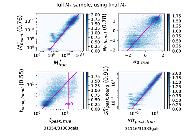
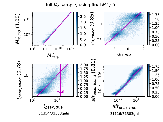
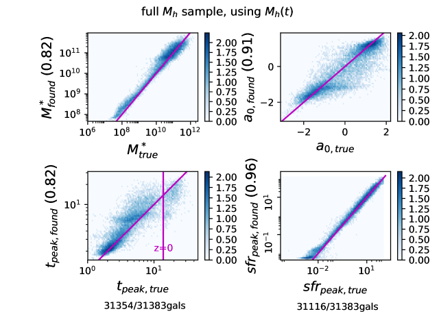
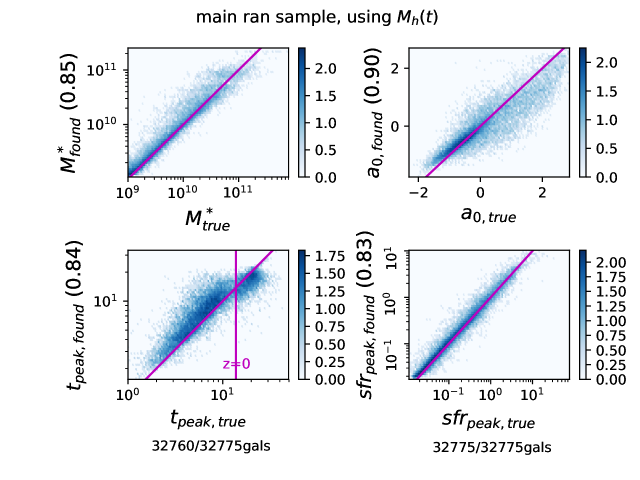
Figure 14: Found and true galaxy properties as listed for the full $M_{h}$ sample (top and lower left) and the main ran sample (lower right), using machine learning. Correlations between found and true properties are listed in parentheses. Training set galaxies were 1/10 of the sample, trimmed by requiring a good $t_{\rm peak}$ fit, and are included in the plot and correlation. Different inputs were explored to obtain final galaxy properties: final $M_{h}$ (upper left), final $SFR,M^{*}$ (upper right), and the main halo history $M_{h}(t)$ for the lower two panels. The color scale shows the log of the number of galaxies in each pixel. Galaxies with $t_{\rm peak,true}>100Gyr$ and $SFR_{\rm peak,true}>100$ were excluded for comparisons between found and true $t_{\rm peak}$ and $SFR_{\rm peak}$ respectively, fractions of galaxies used are given. The fit in Eq.3 was used to calculate the “true” $SFR_{\rm peak,true}$.

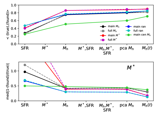
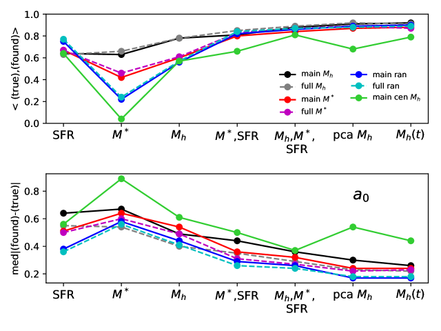
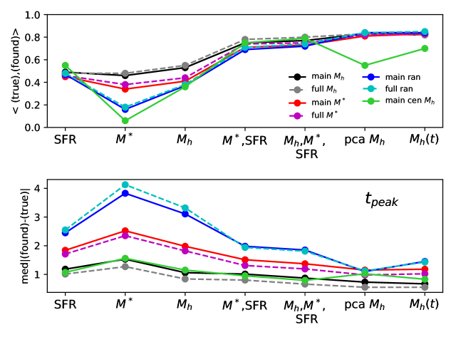
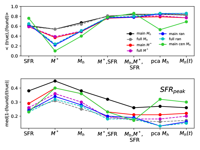
Figure 15: Results for machine learning of galaxy properties: final $M^{*}$ (upper left), $a_{0}$ (upper right), $t_{\rm peak}$ (lower left) and $SFR_{\rm peak}$ (lower right), for each of the 7 samples, with inputs as listed on $x$-axis ($M^{*},SFR,M_{h}$ refer to values at final time). The correlations between true and found values are in each top panel of the 4 sets of panels, the medians of $|\frac{\rm true-found}{\rm true}|$ or the difference $|{\rm found-true}|$, as indicated, are in the bottom panels. Results for full and main histories are similar in many, but not all, cases.

One can go beyond correlations and try to predict $t_{\rm peak}$, $a_{0}$, and more, following the machine learning approach of Kamdar, Turk & Brunner (2016a, b). If machine learning is successful in using smaller numbers of galaxy properties to reproduce properties of the full models, then it can be used to get these properties instead of, for instance, the full semi-analytical models. In addition, the success of obtaining galaxy final and history properties based upon a smaller set of inputs can help guide the choice of properties to include in simplified models.

The details of the methods of Kamdar, Turk & Brunner (2016a, b), in particular, python notebooks, are available publicly at https://github.com/ProfessorBrunner/ml-sims . (See also Xu et al (2013); Ntampka et al (2015) for some other applications of machine learning to galaxy formation in particular. ) Kamdar, Turk & Brunner (2016a) used main galaxy halo histories $M_{h}(t)$ and a few other halo properties as inputs, predicting several final time observables. Again, the semi-analytic models which produce the star formation rate histories use the full, not main, halo history, plus additional dark matter simulation halo information (see, e.g. Fu et al (2013) for a recent summary).

Here, machine learning is applied to predict $t_{\rm peak}$, $\log\sigma_{t}$, $SFR_{\rm peak}$, $a_{0}$,$a_{1}$,$a_{2}$, the final integrated star formation rate, $\tilde{\cal S}(t_{f})$, and final $M^{*}$ for all 7 samples. The method Kamdar, Turk & Brunner (2016a) found most promising for $M^{*}$ and several other properties, extremely randomized trees (Breiman et al, 1984; Geurts, Ernst & Wehenkel, 2006), also gave the strongest correlations between the predicted and true values of $a_{0}$ and $t_{\rm peak}$, although RandomForestRegressor was very close, again, similar to what they found.

For all but the cen $M_{h,{\rm big}}$ sample, the initial training set was a random selection of 10% of the galaxies, subsequently trimmed to keep only those with a good lognormal fit for $t_{\rm peak}$ ($D<0.06$, defined in Eq. 6). For the much larger cen $M_{h,{\rm big}}$ data set, 10,000 random galaxies were chosen (due to limited computing power), and requiring $D<0.06$ left $\sim 7000$ galaxies, closer to 3% of the sample total.

Although main halo histories $M_{h}(t)$ are a key part of the Kamdar, Turk & Brunner (2016a) training set, is it also interesting to understand how well fewer or other inputs recover parameters. This helps to clarify which inputs contain the most predictive power. Inputs considered are:

• final time $SFR$ only

• final time $M^{*}$ only

• final time $M_{h}$ only

• final time $SFR$ and $M^{*}$ together (both observable)

• final time $SFR,M^{*},M_{h}$ together

• first 3 PCA components for $M_{h}(t)$ (again, $M_{h}(t)$ histories normalized to 1 at final time)

• main halo mass histories $M_{h}(t)$ (not normalized)

For all combinations of inputs listed above, correlations between predicted and true values, and median differences or ratios were measured. A few distributions of true versus predicted values are shown in Fig. 14. The training data for these measurements are final $M_{h}$ at upper left, final $SFR,M^{*}$ at upper right, and the main halo histories, $M_{h}(t)$, for different samples at lower left and right.

Summary statistics using all combinations of the inputs to predict $M^{*}$, $a_{0}$, $t_{\rm peak}$ and $SFR_{\rm peak}$ are in Fig. 15. The (fewer than 10% of the) galaxies in the training set are included in the plots and the correlations. The best results came from using the whole (main) halo history, closest to the galaxy information used by Kamdar, Turk & Brunner (2016a). However, many of the variants starting with smaller numbers of inputs exhibited significant success, in particular using the three leading principal components for the halo history.

Some expected trends are visible. For instance, the success of using final $M_{h}$ to predict final $M^{*}$ is presumably due to the stellar mass-halo mass relation. The larger median separations between true and found $t_{\rm peak}$ for the random sample, followed by the $M^{*}$ sample, are likely related to their higher fractions of low $M^{*}$ and thus large $t_{\rm peak}$ galaxies, especially the harder-to-estimate future $t_{\rm peak}$ values. Although the correlations between true and found were similar for the full and main histories, the difference in the median values of the fit parameters sometimes varied more between main and full histories than between samples, for example, for $SFR_{\rm peak}$.

The poorer results for the cen $M_{h,{\rm big}}$ sample seems to be not due to the training of the fits, but from the galaxy distribution in the cen $M_{h,{\rm big}}$ sample itself. Using the full $M_{h}$ sample, e.g., to train a network to predict parameters for the cen $M_{h,{\rm big}}$ sample, gave predictions similarly bad to those found by training the network on the cen $M_{h,{\rm big}}$ sample. More generally, overall correlations between true and found values are strongly dependent on the makeup of the sample. For instance, if only a small range of final halo masses is considered, the correlations between true and found values of $t_{\rm peak}$ decreases, because much of the strength of the correlation between true and found values of $t_{\rm peak}$ is due to machine learning using the final $M_{h}$ dependence of $t_{\rm peak}$ (see Fig. 14).

The mismatch between true and found values of the parameters translates into worse approximations for the fits to the original histories and for the final time stellar mass to star formation rate relation, and a different shape of the scatter around the histories. Results and some comparisons to the earlier direct fits (shown earlier in Fig. 8, Fig. 11, and Fig. 9) are in the appendix, §B. In particular, the number of galaxies assigned the lowest star formation rates ($\leq 10^{-7}M_{\odot}yr^{-1}$) via machine learning never reaches 1/3 of those in the simulation, and in the ran sample is $\leq$ 1% of the simulation number for the lognormal fit.

To summarize, many of the galaxy properties at final time and their main halo histories $M_{h}(t)$ are strongly correlated with the star formation rate history parameters. Machine learning can find fairly good fits to the peak time $t_{\rm peak}$ or leading PCA fluctuation coefficient $a_{0}$ by using the leading 3 principal components of the halo history, or by using the main halo history $M_{h}(t)$. However, although these parameters and final stellar masses are fairly well approximated, the approximations to the true simulation integrated histories and final time values are noticeably worse, and the machine learning determined instantaneous star formation rates at final times have significantly fewer quiescent galaxies in the ran sample (doing slightly better in the samples with more high mass galaxies).

5 Bimodality and beyond

Galaxies are often classified as star forming and quiescent (separated at SSFR $=10^{-12}yr^{-1}$ for the samples here, from considering the SSFR distribution in the simulation outputs). This division can help identify common properties and correlations within the set of star forming or quiescent galaxies, and guide the search for mechanisms which cause transitions between these two categories. Since both $t_{\rm peak}$ and $a_{0}$ give one parameter characterizations for galaxy histories, they can also be used to group galaxies, into subfamilies that share similar integrated star formation rate histories.

Whether a galaxy is star forming or quiescent is, not surprisingly, related to its star formation rate history, and thus to $t_{\rm peak}$ and $a_{0}$, with quiescence tending to imply low $t_{\rm peak}$ (or $t_{1/2}$), and high $a_{0}$, that is, early star formation. However, although related, these separations of galaxy histories are all distinct. The number of galaxies with high $t_{\rm peak}$ and high SSFR matches that of galaxies with low $a_{0}$, and number of galaxies with low SSFR and high $a_{0}$ matches that of galaxies with low $t_{\rm peak}$, but for other pairings of SSFR, $t_{\rm peak}$, and $a_{0}$, the number of galaxies in subfamilies cut on one quantity differs from that in a subfamily found by a cut in another quantity.

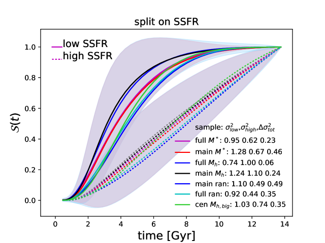
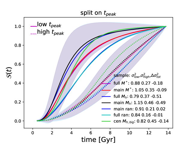
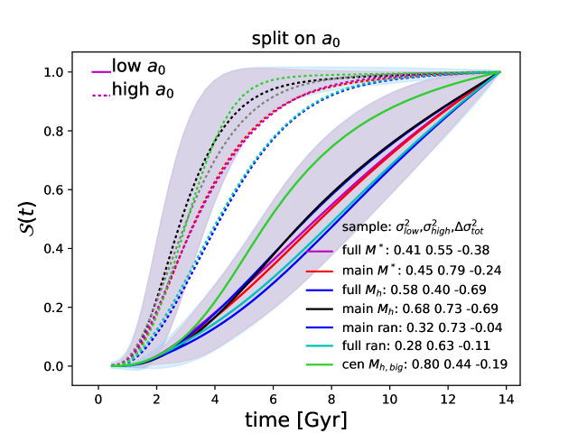
Figure 16: Average integrated star formation rate histories for all 4 samples, split into high and low specific star formation rate (top, $SSFR\lessgtr 10^{-12}yr^{-1}$), $t_{\rm peak}$ (middle) and $a_{0}$ (bottom). Adding a parameter, i.e. splitting into subfamilies, should reduce the scatter ($\Delta\sigma_{\rm tot}$ negative), however the SSFR subfamilies have $\Delta\sigma_{\rm tot}>0$. Thistle shading shows the contribution of the first 3 principal components to the variance, blue (only visible at the edges) the full variance, for the main $M_{h}$ subfamilies only; see text for details of separating into subfamilies.

Although all three quantities can be used to separate galaxy samples, the integrated star formation rate histories of quiescent and star forming galaxies do not separate as well as those with high and low $t_{\rm peak}$ or $a_{0}$. In particular, there is larger scatter around the average values for the quiescent and star forming histories, as shown in Fig. 16. In each panel, each sample’s galaxies are split into high and low $SSFR$ (top panel), $t_{\rm peak}$ (middle panel) and $a_{0}$ (lowest panel). Averages for the high and low subfamilies are shown by lines as indicated. To get a sense of the scatter around the two subfamilies, that for the main $M_{h}$ subfamily is shown in each figure. The subfamily variances around the two averages are shown in blue, and superposed (purple, which almost coincides) are the shapes of the fluctuations due to the first 3 subfamily principal components (within each subfamily). The variance due to the first three principal components at time $t_{i}$ is $\sum_{n=0}^{n=2}<a_{n}^{2}>PC_{n}(t_{i})^{2}$. This gives a visual estimate of the overlap and shows that the two subfamilies again have a few parameters capturing a large amount of scatter around their respective averages.

There are also two quantitative ways of classifying a separation into subfamilies as successful. The first is the change from the total (original) variance to that around the two samples,

$$\Delta\sigma^{2}_{\rm tot}=\sum_{{\rm samples}\;i}\sigma^{2}_{i,{\rm final}}-\sigma^{2}_{\rm initial}<0\;.$$ (10)

When $\Delta\sigma^{2}_{\rm tot}<0$, the separation into subfamilies reduces the total scatter.

The second quantity is the distance between the two subfamily averages, relative to the overlaps of their populations (roughly estimated by the variance around each average). If this ratio is less than one, it suggests that the two populations do not overlap significantly,

$$\frac{\sigma_{0}^{2}+\sigma_{1}^{2}}{|\bar{\cal S}_{0}(t)-\bar{\cal S}_{1}(t)|^{2}}<1\;.$$ (11)

Here, $\sigma_{i}^{2}$ is the variance around each subfamily, with respective average $\bar{\cal S}_{i}(t)$.

In the legends in Fig. 16, $\Delta\sigma^{2}_{\rm tot}$ for each separation is given for each galaxy sample and separations. Although the SSFR separation is fixed, the separations for $t_{\rm peak}$ and $a_{0}$ are chosen by scanning through values to minimize $\Delta\sigma^{2}_{\rm tot}$ and the overlap, Eq. 11. For the SSFR split, $\Delta\sigma^{2}_{\rm tot}$ and the overlap between the regions which lie in the scatter of both average paths are larger (this is true for all 7 samples). Subfamilies of galaxies sharing high or low $t_{\rm peak}$ or high or low $a_{0}$ have more distinct integrated star formation rate histories.

5.1 Subsets of galaxy histories

As splitting on specific star formation rate does not separate galaxy histories into distinct families as well as using $t_{\rm peak}$ or $a_{0}$, and the distribution of these latter two parameters (Fig. 3) is not necessarily bimodal, it seems possible to group galaxies into more than two subfamilies, with each subfamily sharing similar integrated star formation rate histories. One motivation for this is to compare properties of galaxies lying in different subfamilies, besides the parameters used to sort into subfamilies. This might be useful in identifying shared trends in subfamilies or general physical causes of certain properties. For instance, if massive galaxies are present in several different subfamilies, one might ask what properties caused their different integrated star formation rates, in spite of their sharing the same final halo mass? These subfamily classifications can serve as starting points for such lines of investigation.

Here a first step is taken in exploring separations into many subfamilies. Whether subfamilies are well separated can again be decided by comparing whether the final sum of scatters around each subfamily is smaller relative to the that of the full sample around its average ($\Delta\sigma^{2}_{\rm tot}<0$, Eq. 10) and whether adjacent subfamilies are sufficiently separated,

$$\frac{\sigma_{i}^{2}+\sigma_{i+1}^{2}}{|\bar{\cal S}_{i}(t)-\bar{\cal S}_{i+1}(t)|^{2}}<1\;.$$ (12)

The split is now into many ($i=1,\dots N$) subfamilies, each with individual averages $\bar{\cal S}_{i}(t)$.

The wide range of histories shared by galaxies with the same final stellar mass was noted by Pacifici et al (2016), who separated quiescent and star forming galaxies and then stacked star formation rate histories within these categories based upon stellar mass. The averages $\bar{\cal S}_{i}(t)$ and variances around them for six stellar mass families (quiescent galaxies only, i.e. SSFR $\leq 10^{-12}\;yr^{-1}$) are shown in in Fig. 17, top, for the main ran sample. The other samples are similar. In addition to the large scatter overlaps between average histories for the subfamilies, i.e., Eq. 12 does not hold, the sum of scatters around the individual $\bar{\cal S}_{i}(t)$ is much larger than original scatter around the single average history ($\Delta\sigma^{2}_{\rm tot}$ is listed above the panel).

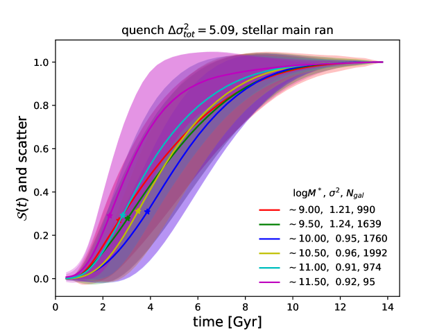
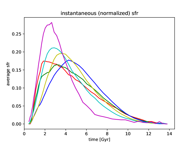
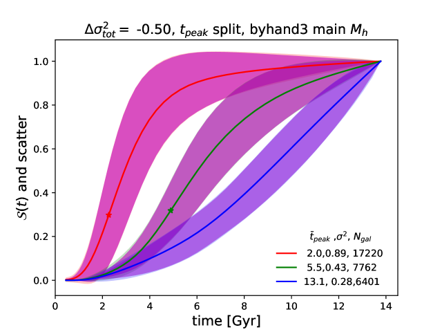
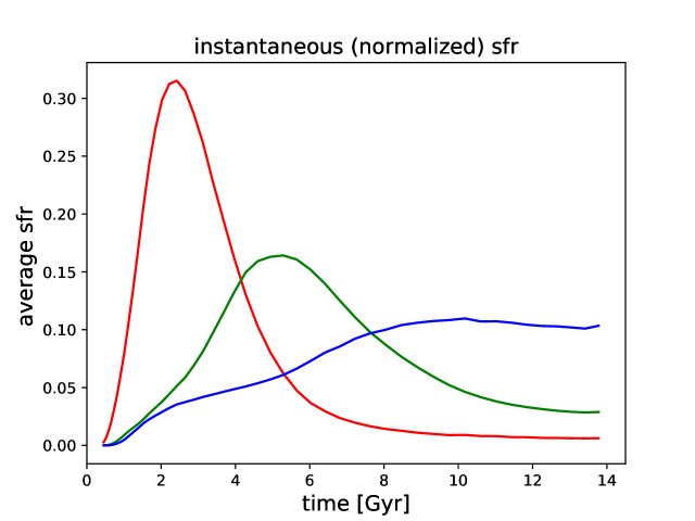
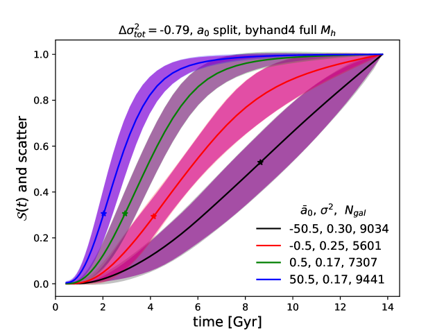
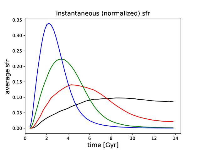
Figure 17: Three examples of splits of integrated histories into families. Top: quenched galaxies in the main ran sample (SSFR $<10^{-12}yr^{-1}$), split by final stellar mass as in Pacifici et al (2016). Middle: the main $M_{h}$ sample split by $t_{\rm peak}$. Bottom: the full $M_{h}$ sample split by $a_{0}$. In each, $\Delta\sigma^{2}_{\rm tot}$, Eq. 10, is shown at top. At left, lines are the average in each subfamily, stars are the lognormal fit $t_{\rm peak}$ to these averages. The dark shaded region is the variance around each average history due to the first 3 principal components in each subfamily, as in Fig. 16. The light shaded region (indistinguishable in most places, the first 3 principal components dominate the scatter) is the corresponding full variance. At right are the averages of the instantaneous star formation rates in each subfamily (normalized by each galaxy’s final integrated star formation rate). For the stellar mass separated sample, the different subfamilies overlap significantly; final stellar mass is not that closely correlated with galaxy integrated star formation rate history. Using $t_{\rm peak}$ and $a_{0}$ gives better separations into subfamilies.

In comparison, $a_{0}$ and $t_{\rm peak}$ can separate integrated histories more cleanly. Two examples are shown in Fig. 17. The middle example splits all galaxies based upon $t_{\rm peak}$, the lower example, using $a_{0}$.

An exhaustive study of possible separations into categories is beyond the scope of this note. An assortment of subfamily splits were tried. Their $\Delta\sigma^{2}_{\rm tot}$ values are compared in appendix §C, and those tried which reduced the total scatter also had subfamilies separated enough according to Eq. 12. Some general features were noted, for instance, when using $t_{\rm peak}$ to determine subfamilies, galaxies with $t_{\rm peak}>$7 Gyr had integrated histories which seemed too close together to lie in different subfamilies. One other way of separating integrated histories was also considered, suggested by Pacifici et al (2016), a quenching time $t_{q}$. In the few examples explored, $t_{q}$ did not seem to work as well as $t_{\rm peak}$ or $a_{0}$, for instance in terms of $\Delta\sigma^{2}_{\rm tot}$, however, again, an exhaustive comparison was not made, and the definition could also be refined.

Once a sample is split according to $a_{0}$ or $t_{\rm peak}$, galaxies which share similar integrated star formation rate histories can be compared in terms of other properties, such as final time $M^{*}$ or $M_{h}$, for instance, to look for reasons that a common final time property is associated with different subfamilies, when that occurs. Distributions of several properties for the galaxies in the 3 or 4 subfamilies of Fig. 17 are compared side by side in the appendix, §C, as examples.

In summary, as might be expected, splitting integrated star formation rates of galaxies according to whether they are star forming or quiescent doesn’t separate their histories as well as splitting based upon their lognormal fit $t_{\rm peak}$ or $a_{0}$. For a bimodal split, using $a_{0}$ to sort each galaxy reduced the total scatter more generically than using $t_{\rm peak}$, however, for splits into several subfamilies, both $t_{\rm peak}$ and $a_{0}$ can be seen to reduce the full scatter and give what seem to be reasonably separated histories. A few other general trends seemed to occur. For instance, all galaxy integrated star formation rate histories with a fitted $t_{\rm peak}\gtrsim 7$ Gyr tended to have large overlap with each other. And again, as $a_{0}$ dominates the scatter around the average history, it is not surprising that subfamilies split via its value are less likely to overlap than those split via final time properties. These separations may be useful as starting points for comparing galaxies which share one property but not another in a simulation (for example, $t_{\rm peak}$ but not final $M^{*}$, or final $M_{h}$ but not $a_{0}$).

6 Summary, Discussion and future directions

In this note, two different methods for parameterizing integrated star formation rate histories were considered: a fixed lognormal form (following Gladders et al (2013); Diemer et al (2017)) and a PCA approximation, treating all histories as the ensemble average plus a combination of the leading three fluctuations (principal components) around it. The lognormal parameterization treats the star formation rate history as having a peak at a certain time, plus a width with a fixed shape, while PCA views all histories as fluctuations around one average history (independent of whether the galaxy is quiescent or not), plus fluctuations of fixed shape and coefficients varying in size and sign. The PCA approximation, using the first 3 principal components, has one more parameter than the lognormal fit, and is more closely tied to the properties of the ensemble of galaxies it describes, as the principal components and the average history around which they fluctuate are both determined using the galaxy sample itself.

These fits were explored with data from the Henriques et al (2015) model built upon the Millennium simulation Springel et al (2005); Lemson et al (2006). To illustrate how to compare samples (or more generally models), four sets of simulated galaxy histories were created: one approximately uniform in $\log M_{h}$, one approximately uniform in $\log M^{*}$, one randomly selected, and including all final time central galaxies in massive halos.

The samples of galaxies were characterized by their lognormal fit parameters (especially $t_{\rm peak}$) and by their average histories, PCA fluctuations, and distributions of the fluctuation coefficients (especially $a_{0}$). For the PCA approximation, the shapes of the averages and fluctuations were similar across different samples, with most variations between samples easily interpreted as due to changes in the number of galaxies with high final halo mass (expected to quench earlier). The first 3 PCA components captured a large fraction of the scatter around the average history for every sample. The lognormal and PCA fits have correlated leading parameters, especially for galaxies with an early $t_{\rm peak}$ and high $a_{0}$. The lognormal fit parameter $t_{1/2}$, when a galaxy dropped to half of its peak star formation rate, was also strongly correlated with $a_{0}$.

Star formation rates of both the main (following one galaxy through time) and full (including all the galaxies which eventually merge to form the the final galaxy) integrated star formation rate histories were considered for 3 of the 4 samples. The full histories have an earlier $t_{\rm peak}$ in the lognormal fit, and smaller variance around the average history in PCA. The full and main histories differed more strongly for samples with larger numbers of high final mass galaxies, Different samples (or models) of galaxies can be compared via parameters of the lognormal fit ($t_{\rm peak},\sigma_{t},A$, and the average relation $\sigma_{t}\approx at_{\rm peak}^{b}$) and by the PCA fit parameters ($a_{0},a_{1},a_{2},\tilde{\cal S}(t_{f})$), the average history of the sample and its PCA basis fluctuations and the variance in the fluctuations.

Two fixed time properties were studied in more detail. The instantaneous star formation rates in the simulations were compared to that given by the fits. The lognormal fit worked better in tracing the distribution of the instantaneous star formation rate at the final redshift (in particular, it was difficult to get the correct number of green valley galaxies in the PCA approximation, even when many principal components were included). It is possible that even with the visible differences from the true (i.e. simulation) values that the fits can provide useful approximate star formation rates, depending on what the rates are used for; the average deviation between the fit and simulated values, over time steps, is zero by construction for the PCA approximation, and small for the lognormal fit.

Secondly, the peak star formation rate halo mass $M_{h,{\rm peak}}$ is bimodal as a function of $t_{\rm peak}$. (It is not seen in the high final mass cen $M_{h,{\rm big}}$ sample which excludes low mass halos by construction.) Downsizing is also evident on the dominant (higher $M_{h,{\rm peak}}$) branch. It would be interesting to understand what is happening with the lower $M_{h,{\rm peak}}$ galaxies. Perhaps environmental effects are starving their growth, for example. It would also be interesting to understand if this feature appears in other galaxy formation models and in nature.

The parameterizations for both fits were correlated with final time properties ($M^{*},M_{h}$ and SFR), and with properties of the galaxy main halo histories. Machine learning, following Kamdar, Turk & Brunner (2016a), was used to estimate the PCA and lognormal approximation parameters, using a range of inputs, including just the final halo mass and the main halo history $M_{h}(t)$. (The galaxy histories are the product of a detailed and complex semi-analytic model, following all halo and subhalo contributions and many physical properties of a galaxy throughout time, and so are automatically related to the full, rather than main, halo histories.) The final halo mass could already give a significant correlation between the true and found values of several fit parameters. The first 3 principal components of $M_{h}(t)$ almost worked as well as $M_{h}(t)$ itself in predicting fit parameters, and the true and found values of several quantities were highly correlated. However, the machine learning predicted final time star formation rates were even further from their simulation (true) values than the original fits. Machine learning shows that a relation can be found, but does not detail the relation, aside from providing importances. For these galaxy halo histories, it seemed that halo masses at a wide range of times in the history were important for predicting final values. It suggests promise for linking halo main histories directly to star formation rate histories through these parameterizations, perhaps in a simplified galaxy formation model.

Using the leading parameter of either approximation, $a_{0}$ or $t_{\rm peak}$, better separates galaxies into subfamilies with similar histories than using whether a galaxy is quenched or star forming at final times. However, once a continuous parameter is used to separate histories, there is no obvious reason to only split galaxies into two groups. Separations into more families of galaxy histories were explored. Many were found which both reduced overall scatter and had subfamilies separated further than the variances around each subfamily average. These might be useful to compare galaxies with similar histories but different final properties or vice versa, to help identify which changes create these different populations within a single galaxy formation model, or to compare between models.

All of these calculations were done within the context of the Henriques et al (2015), or L-galaxies, semi-analytic model built upon the Millennium simulation. The lognormal fit was applied to the Illustris simulation in the Diemer et al (2017) paper inspiring this work. Illustris incorporates different physics, has a different number of time steps, and better (using the measure $D$ in Eq. 6) lognormal fits to its histories than the fits to the histories here. Both of these simulations have some disagreement with observations, as noted earlier, for instance, one comparison has found that L-galaxies quenches too quickly and Illustris not enough (Bluck et al, 2016), which was seen, for example, in comparison of their $\sigma_{t}(t_{\rm peak})$ relations. It would be interesting to compare these approximations between other simulations and models.

Not only can galaxy formation models be changed, other definitions of peak time may also be more effective at either separating the integrated star formation rate histories into families, or matching the instantaneous star formation rates. For instance, there are different fits such as the double power law fit of Behroozi, Wechsler & Conroy (2013b) studied in Diemer et al (2017), which has less scatter in many cases, but also many singular fits at least when tried for the galaxy histories studied here, see also Gladders et al (2013); Carnall et al (2017); Martinez-Garcia et al (2018) for examples of other studies of a variety of functional forms. (Carnall et al (2017) identify several distinct star formation history shapes, depending upon the particular galaxy.) Two other obvious possibilities for special times, even within the lognormal fit definition, are $t_{1/2}$ and the quenching time. The quenching time also requires the stellar mass, time, and choosing a definition and width of the star forming main sequence, so it was not pursued in detail here.

In summary, these two ways of viewing galaxy integrated star formation rate histories provide examples of how to distill some of the huge variation and complexity of galaxy formation into a few characteristics of galaxy histories and their populations. These characteristics often have simple meanings and can be compared between models, and ideally, eventually to physical mechanisms. In the examples here, the variations between these characteristics revealed the different underlying mass distributions in the subsamples. Comparing the average histories, fluctuations, distribution of parameters (and their relations to each other, e.g., here for the lognormal fit), separations into subfamilies and other properties across simulations may allow identifying properties charaterizing the full samples, and thus the models which created them. These properties may not be evident in the detailed prescriptions for the individual galaxies, but instead emerge in the samples, and perhaps in observations, as a whole.

Appendix A The cen $M_{h,{\rm big}}$ sample

The cen $M_{h,{\rm big}}$ sample is based upon the sample used by Kamdar, Turk & Brunner (2016a), who took central galaxies which had $M_{h}\leq 10^{12}M_{\odot}$ at final times, and found that using main halo histories plus some other histories and parameters as inputs for machine learning gave a $\sim$ 88% correlation between predicted and true $M^{*}$. For their machine learning, they use information beyond $M_{h}(t)$ as input for the learning algorithm, including circular velocity $V_{\rm max}(t)$ and velocity dispersion $V_{\rm disp}(t)$.

But there are also differences with their $M_{h}(t)$ sample from cen $M_{h,{\rm big}}$. In particular, their outputs are traced back to $z=5.7$, while here the starting time is $z\sim 10$ (they had 45 outputs compared to the 48 here). They also used a different, earlier, semi-analytic model (Guo et al, 2010) from the Millennium database. For machine learning, it seems the most important difference is that their sample was trimmed in two ways. It was trimmed explicitly reject outliers. It was also trimmed implicitly through the SQL query to reject the $\sim$7% of the halos meeting the final halo mass and central galaxy criteria which were not present at all time steps. That is, they used “INNER JOIN” rather than “FULL OUTER JOIN” used here. This may have resulted in a sample which was not only better behaved, but easier to model via machine learning.

Appendix B Machine learning fits

Machine learning, discussed in §4.3 in the text, was applied to all 7 samples, using $M_{h}(t)$ to predict the parameters $t_{\rm peak}$, $\sigma_{t}$, $A$, $a_{0}$, $a_{1}$, $a_{2}$, $\tilde{\cal S}(t_{f})$ and the final time $M^{*}$. Below, the resulting fits to the integrated star formation rates are compared to the simulation outputs, in direct parallel to the comparison of the direct fits with the simulation outputs in §3.3.2 and §3.3.3.

B.1 Goodness of approximations using ML parameters

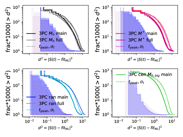
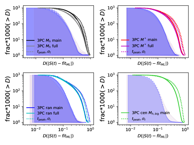
Figure 18: Separation between simulated integrated star formation rate histories ${\cal S}(t)$ and their approximations using machine learning to find $a_{0},a_{1},a_{2}$ (solid lines) or $t_{\rm peak},\sigma_{t}$ (dashed lines). The top four panels give $d^{2}=|{\cal S}(t)-fit_{ML}|^{2}$, while the bottom panels give $D$ (Eq. 6), as in Fig. 8. The shaded regions are the corresponding distributions for the direct fits to the simulation histories, from Fig 8.

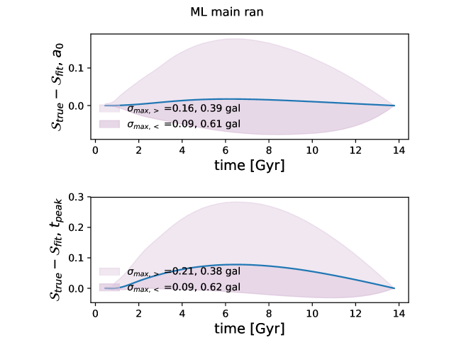
Figure 19: Average difference $\langle{\cal S}_{\rm true}(t)-{\cal S}_{\rm fit}(t)\rangle$, solid line, and its scatter, shaded, for the machine learning PCA fit (top) or lognormal fit (bottom), in the main ran sample. The simulation gives ${\cal S}_{\rm true}(t)$. This can be compared to the average and scatter from the direct fits shown in Fig. 9 in the main text. Again, the shaded regions are one standard deviation, calculated separately for galaxies with ${\cal S}_{\rm true}(t)-{\cal S}_{\rm fit}(t)$ above or below the average. The scatter is much larger in the machine learning fits, and has changed shape. Relative to the direct fits, the standard deviations have increased from $\leq 0.05$ to 0.15-0.20 (PCA), and from $\leq 0.07$ to 0.19-0.24 (lognormal). Note the fit on average tends to overestimate rather than underestimate ${\cal S}_{\rm true}$, unlike the earlier fit.

Just as for the original fits in 3.3.2, the machine learning fits can be compared to the simulated histories using $d^{2}$ and $D$. These are shown in Fig. 18, with the original distributions from Fig. 8 shown as shaded regions for comparison. The shading gives an estimate of how much the fits degrade when machine learning is used. For the direct fits to the simulations, the squared separation between the simulated and direct fits, i.e., $d_{t_{\rm peak}}^{2}$ and $d_{\rm PCA}^{2}$, were 22%- 53% correlated. The correlations of scatter from the true values, between the two kinds of approximations, increased to 80%-92% for the machine learning fits based upon $M_{h}(t)$. That is, large or small separations between the actual history and their machine learning reconstructions tended to occur together for both kinds of approximations, perhaps indicating something about which $M_{h}(t)$ were harder/easier to associate with the correct fit parameters.

A slightly more detailed characterization of the difference between the approximations from machine learning and the simulated ${\cal S}(t)$, similar to Fig. 9, is shown in Fig. 19. This again shows, for the ran sample, the average deviation between true and fit ${\cal S}(t)$ at each time step, and standard deviations from it (again calculated separately for above and below). The average deviations when using machine learning fits rather than direct fits are much larger, the standard deviations go up by a factor of $\sim 3$ and have a different shape. Note the machine learning fit on average has a larger bias, and a larger tendency to overestimate rather than underestimate ${\cal S}_{\rm true}$.

This shape is similar for all samples and for both the lognormal and PCA fits. The average deviation of the fit and the size of the scatter around this average deviation are also much bigger for the machine learning fits.

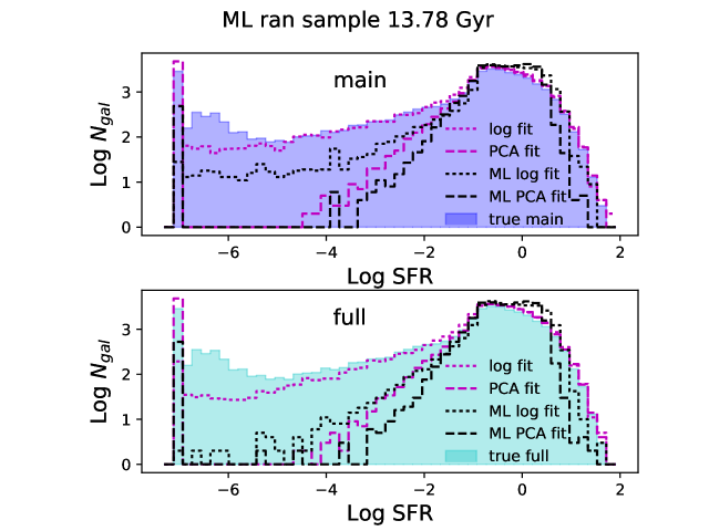
Figure 20: Final time star formation rates in the ran simulation (top panel uses main integrated star formation rate history fits, bottom panel uses full integrated star formation rate history fits). The filled in region shows the simulation (true) final star formation rate distributions. The star formation rates for the direct fits to the histories, shown earlier in magenta in Fig. 10, are shown again here. The machine learning fits are in black. Dotted lines correspond to the lognormal fit and dashed lines to the PCA fit. Again, galaxies with negative star formation rates in the PCA fit are set to $10^{-7}M_{\odot}yr^{-1}$ along with any other galaxies with star formation rates $<10^{-7}M_{\odot}yr^{-1}$. The machine learning fits tend to give a narrower peak at high star formation rate.

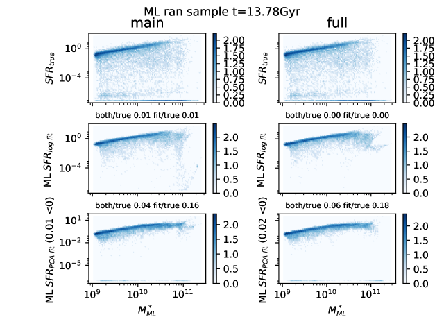
Figure 21: Stellar mass versus star formation rate at redshift zero from machine learning for $M^{*}$ and the lognormal fit (middle panels) and the PCA fit (bottom panels), compared to the actual distribution in the simulation (top panels). This is the same comparison, for the same ran sample, as shown in Fig. 11, however in that case, the fits were direct, rather than via machine learning. At left, the fit to the main star formation rate history is used, at right, the fit to the full star formation history is used. Again, galaxies with negative star formation rates in the PCA fit are counted and then set to $10^{-7}M_{\odot}yr^{-1}$ along with any other galaxies with star formation rates $<10^{-7}M_{\odot}yr^{-1}$. Other quantities are defined as in Fig. 11. See text for more discussion.

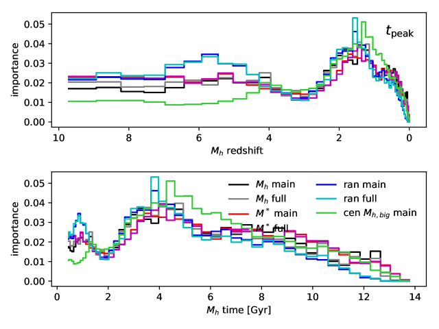
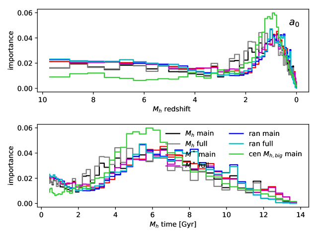
Figure 22: Importance of different times in $M_{h}(t)$, for machine learning predictions for $t_{\rm peak}$ and $a_{0}$ (top, redshift space, bottom, time). Different colored lines are different samples. Values of $M_{h}(t)$ around 4-5 Gyr seem to have the most weight.

B.2 Approximating final time star formation rate

For the final time $SFR(M^{*})$ predictions, Fig. 15 shows the correlations between true and found for the final $M^{*}$ machine learning predictions. Two other $M^{*}$ tests not shown are successful: the stellar mass to halo mass relation, considered in Kamdar, Turk & Brunner (2016a) and the stellar mass function (well reproduced except for losing some galaxies at the high mass end). However, the stellar mass to star formation rate relations are worse because of the final time star formation rate discrepancies, shown in Fig. 20. This can be compared to Fig. 10 in §3.3.3; the black lines give the machine learning predictions, while the magenta lines show the earlier predictions using the direct fits. The machine learning prediction for the number of galaxies in the green valley decreases for both fits for the ran sample, but behaves differently in other samples. All samples show some increase of galaxies with fairly high star formation rates above the number in the simulation when the rates are found using machine learning fits.

The resulting stellar mass to star formation rates, the machine learning version of Fig. 11, are shown in Fig. 21. Just as in Fig. 11 the simulation result is at top, and the fits (this time from machine learning) are below. The fractions of negative star formation rates for the PCA fit are again given on the $y$-axis on the lowest row, after which all galaxies with SFR $\leq 10^{-7}M_{\odot}yr^{-1}$ are assigned to the minimal SFR $=10^{-7}M_{\odot}yr^{-1}$. These minimal SFR galaxies are compared in the simulation and the fits: the numbers of low star formation rate galaxies common to the fit and the simulation (“both”), in the simulation (“true”) and in the fit (“fit”) are compared in the ratios (“both/true”), (“fit/true”), shown in each fit panel. In the lower panel, again all galaxies with SFR $\leq 10^{-7}M_{\odot}yr^{-1}$ are plotted as galaxies with SFR $=10^{-7}M_{\odot}yr^{-1}$. The ran sample lognormal fit from machine learning has the smallest number of “fit/true” low star formation rate galaxies, but this number does not go above 0.31 for either fit among any of the samples.

The machine learning fits also provide the “importance” of difference components of the input in producing the final results. Examples of this importance for $t_{\rm peak}$ and $a_{0}$ predictions are in Fig. 22, in terms of redshift in the top panel, and time on the bottom panel, and are hard to interpret. Many individual redshifts between 0 and 2 seem to have more importance than earlier times, even though many of the galaxies have their peak time well before redshift 2 (at $\sim 2$ Gyr, Fig. 22). This is likely related to the fit information available when star formation declines at these later times.

Appendix C Separating galaxy histories into many subfamilies

As discussed in §5, integrated star formation rate histories can be separated into many different subfamilies, once a continuous parameter such as $t_{\rm peak}$ is assigned to each history. A variety of different splits were tried, with $\Delta\sigma^{2}_{\rm tot}$, Eq. 10, and the overlaps, Eq. 12, compared for each. Subfamilies were divided according to quenching time, $t_{\rm peak}$ and $a_{0}$, changing the number of subfamilies and dividing values of the parameters. Some splits were uniform, others were based on different regions visible in figures such as Fig. 7. (Uniform splits for $t_{\rm peak}$ grouped all histories with $t_{\rm peak}\gtrsim 7.5$ Gyr together as they always significantly overlapped.) A sampling of how the scatter changes in different subfamily choices, and 2 examples of galaxy properties in the different subfamilies are given in this section. A full exploration of all possible subfamilies is beyond the scope of this work.

For this small set of assorted subfamilies, a chart of $\Delta\sigma^{2}_{\rm tot}$ as a function of number of subfamilies is shown in Fig. 23 (for splits into subfamilies with $\Delta\sigma^{2}_{\rm tot}<4$). The divisions based upon $M^{*}$ and SSFR discussed in §5 are also included.

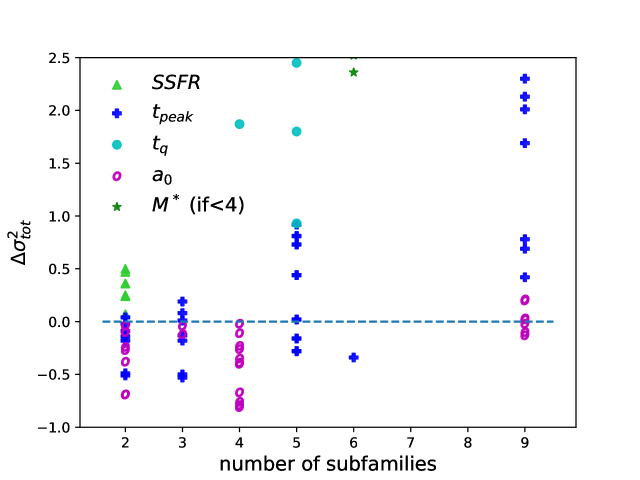
Figure 23: The change in total variance, $\Delta\sigma^{2}_{\rm tot}=\sum_{i}\sigma^{2}_{i,{\rm final}}-\sigma^{2}_{\rm initial}$, for galaxy samples split into different numbers of subfamilies (numbers noted on the $x$-axis), for different parameter values and different samples (i.e., $M_{h}$, $M^{*}$, ran, cen $M_{h,{\rm big}}$). The average histories for the splits into two subfamilies are in Fig. 16. Splits were uniform or guided by features in the individual or joint distributions of $t_{\rm peak},a_{0},t_{q}$; the divisions based upon $M^{*}$ and SSFR mentioned in the text are also included. Subfamilies with $\Delta\sigma^{2}_{\rm tot}\geq 4$ are not shown. The more negative $\Delta\sigma^{2}_{\rm tot}$, the more the split into subfamilies reduces total scatter. For all samples with $\Delta\sigma^{2}_{\rm tot}<0$ shown here, the scatter between adjacent subfamilies was also less than the distance between the corresponding average integrated star formation rate histories, i.e., satisfying Eq. 12.

In this small sample, splitting integrated star formation rate histories based upon $a_{0}$ again tended to succeed more often than splitting on the basis of $t_{\rm peak}$ or $t_{q}$, perhaps because $a_{0}$ is the coefficient of the largest fluctuation around the average history. However, these examples do not preclude better (in terms of $\Delta\sigma^{2}_{\rm tot}$ and Eq. 12) separations in terms of $t_{\rm peak}$ or $t_{q}$.

The galaxies in the different subfamilies can be compared in terms of their average history properties (stellar mass, halo mass and main and full integrated star formation rates), and other properties. Two examples are shown in Fig. 24 and Fig. 25. For these subfamilies, the average integrated star formation rate histories, scatter around these averages, and instantaneous star formation rates are in the bottom two panels in Fig. 17. Fig. 24 corresponds to properties of the 3 subfamilies separated using $t_{\rm peak}$, for the full $M_{h}$ sample, and Fig.  25 corresponds to the separation of galaxies into 4 subfamilies using $a_{0}$, in the main $M_{h}$ sample.

Figure 24: Properties of the galaxies sorted by the $t_{\rm peak}$ separations producing the average integrated and instantaneous star formation rate histories in the middle row of Fig. 17. Each column corresponds to one subfamily, with sample galaxies chosen according to the $t_{\rm peak}$ range listed at top. The highest row shows the average main integrated SFR (solid blue), full integrated SFR (dashed blue), $M_{h}$ (solid black) and $M^{*}$ (green stars) histories. Each type of history is normalized to the same final value, described in the text. The scatters are not rescaled with the final values, so sizes and shapes of scatters can be compared directly across subfamilies, and the vertical axis is shared across all columns on the top row. Histories are all as a function of time, listed in Gyr along the $x$-axis. The magenta vertical line shows the average peak time for the each subfamily. In the second row, the solid line shows the $a_{0}$ distribution for the subfamily, with light purple shading showing the full sample distribution. This breaks down the relation between $a_{0}$ and $t_{\rm peak}$. The third row shows the logarithm of number of galaxies with a given final log $M^{*}$ and SFR. Galaxies with SFR=0 are set to $SFR=10^{-7}M_{\odot}yr^{-1}$. Solid dark lines in the fourth and fifth rows give the log of the number of galaxies with a given final $M^{*}$ and final $M_{h}$ for each subfamily, along with the full distribution, shaded in light purple. The distribution of satellites in the lower two panels is shown as a dashed red line.

In each plot, each column is a different subfamily, and each row focuses the distribution of the same property or properties.

• The top row panel shows average histories for $M^{*}$, $M_{h}$, and the full and main integrated star formation rate. (These are full and main histories in subfamilies determined by $a_{0}$ or $t_{\rm peak}$ from either the main or full integrated star formation rate histories.) The main integrated star formation rate is rescaled to have final value 1. The other histories are rescaled to have the same final value, corresponding to the median values of $\tilde{\cal S}_{\rm full}(t_{f})/\tilde{\cal S}_{\rm main}(t_{f})$ for the full integrated star formation rate histories, $1.868M^{*}(t_{f})/\tilde{\cal S}_{\rm main}(t_{f})$ for the stellar mass histories, and $M_{h}(t_{f})/(100\tilde{\cal S}_{\rm main}(t_{f}))$ for the halo mass histories.

  The prefactor for the stellar mass history rescaling is to take out the stellar ageing; if the stellar mass history and main integrated star formation rate history roughly coincide, then almost all the star formation occurs in the main history, i.e. in situ. This is also seen in the difference between the full (dashed line) and main (solid line) integrated star formation rate histories; these two lines overlap if the median full and main histories overlap after this rescaling. As might be expected, this overlap occurs more for low $a_{0}$ or high $t_{\rm peak}$, corresponding to the lowest final $M^{*}$ and final $M_{h}$ galaxies. These galaxies are not expected to gain much stellar mass through mergers, tending to be small and star forming (or quenched satellites). The vertical solid line is the $t_{\rm peak}$ for the average integrated star formation rate history for each subfamily.

  The shading around the main halo mass histories and the main stellar mass histories are the 3 principal components of scatter (purple) and the full variance (blue, at edges) around the galaxy histories. These scatters are rescaled to histories with a final value of 1, so that their relative size can be compared directly between different columns, similarly, the vertical scales for the top row are identical for all columns.

• The solid lines in the second rows show the distribution of $a_{0}$ (for the sample split on $t_{\rm peak}$) or $t_{\rm peak}$ (for the sample split on $a_{0}$), to see how well the cut in one quantity corresponds to a cut in the other. The shaded region shows the full sample distribution of $a_{0}$ or $t_{\rm peak}$ respectively.

• The next three rows are final time properties, showing the stellar mass to halo mass, final stellar mass and final halo mass of galaxies in each subfamily. The shaded regions show the full sample distribution of these quantities. For final $M^{*}$ and final $M_{h}$, the distribution for satellites is also shown separately.

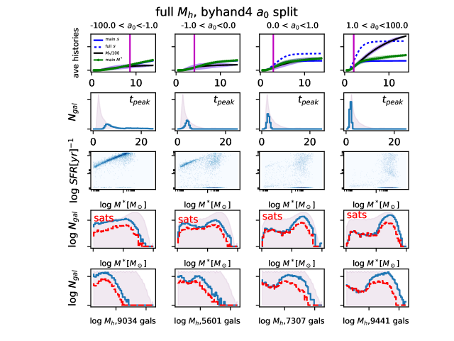
Figure 25: Final time properties of the galaxies in subfamilies corresponding to the $a_{0}$ separation with average integrated and instantaneous star formation rate histories shown in the bottom row of Fig. 17. Lines and colors are as in Fig. 24 above, except for the second row. In this case, as $a_{0}$ is used to separate the histories into subfamilies, the $t_{\rm peak}$ distribution of each subfamily is given, with the full distribution shown as a shaded region. In the bottom two rows, the subfamily (2nd column) which is bimodal in $M_{h}$ and $M^{*}$ can be further split into two samples by using $a_{1}$ or $a_{2}$, both of which are correlated with high or low final $M^{*},M_{h}$ in this subfamily.

These figures compare different properties of the subfamilies which have different integrated star formation rate histories. Similar final properties are often spread across several subfamilies. For instance, galaxies with moderately high final $M^{*}$ can lie in 3 of the 4 subfamilies split using $a_{0}$ in Fig. 25, with different contributions from, for instance, mergers. These comparisons may give another angle on trying to disentangle contributing factors to the formation of galaxies. Similarly, galaxies with early peaks in star formation rate can often span a wide range of final stellar masses. Again, the hope would be that these comparisons would help identify cases where some features are shared and others differ, which could motivate searches for physical causes of either the differences or the similarities. These simpler questions may give useful angles for approaching the wide diversity of properties and galaxy histories produced by galaxy formation models.

References

- Abramson et al (2016) Abramson, L.E., Gladders, M.D., Dressler, A., Oemler, A.,Jr, Poggianti, B., Vulcani, B., 2016, ApJ, 832, 7
- Agarwal, Dave & Bassett (2017) Agarwal, S., Dave, R., Bassett, B.A., 2017, arXiv:1712.03255
- Angulo & White (2010) Angulo, R.E., White, S.D.M., 2010, MNRAS, 405, 143
- Angulo & Hilbert (2015) Angulo, R.E., Hilbert, S., 2015, MNRAS, 448, 364
- Behroozi et al (2013a) Behroozi, P.S., Marchesini, D., Wechsler, R.H., Muzzin, A., Papovich, C., Stefanon, M., 2013a, ApJL, 777, 10
- Behroozi, Wechsler & Conroy (2013b) Behroozi, P.S., Wechsler, R.H., Conroy, C., 2013a, ApJ, 770, 57
- Bluck et al (2016) Bluck, A.F.L., et al., 2016, MNRAS, 462, 2559
- Breiman et al (1984) Breiman L., Friedman J., Stone C. J., Olshen R. A., 1984, Clas- sification and regression trees. CRC press
- Carnall et al (2017) Carnall, A.C., McLure, R.J., Dunlop, J.S., Dave, R., 2017, arxiv:1712.04452
- Cohn & Van de Voort (2015) Cohn, J.D., van de Voort, F., 2015, MNRAS, 446, 3253
- Dekel et al (2013) Dekel, A. Zolotov, A., Tweed, D., Cacciato, M., Ceverino, D., Primack, J.R., 2013, MNRAS, 435, 999
- Diemer et al (2017) Diemer, B., Sparre, M., Abramson, L.E., Torrey, P., 2017, ApJ, 839, 26
- Eales et al (2018) Eales, S., et al, 2018, MNRAS, 473, 3507
- Fu et al (2013) Fu, J., et al, 2013, MNRAS, 434, 1531
- Geurts, Ernst & Wehenkel (2006) Geurts P., Ernst D., Wehenkel L., 2006, Machine learning, 63, 3
- Gladders et al (2013) Gladders, M.D., Oemler, A., Dressler, A., Poggianti, B., Vulcani, B., Abramson, L., 2013, ApJ, 770, 64
- Guo et al (2010) Guo, Q., White, S., Boylan-Kolchin, M., De Lucia, G., Kauffmann, G., Lemson, G., Li, C., Springel, V., Weinmann, S., 2011, MNRAS, 413, 101
- Guo et al (2013) Guo, Q., White, S., Angulo, R. E., Henriques, B., Lemson, G., Boylan-Kolchin, M., Thomas, P., Short, C., 2013, MNRAS, 428, 1351
- Hearin & Watson (2013) Hearin, A.P., Watson, D.F., 2013, MNRAS, 435, 1313
- Henriques et al (2015) Henriques, B. M. B., White, S. D. M., Thomas, P. A., Angulo, R., Guo, Q., Lemson, G., Springel, V., Overzier, R.,2015, MNRAS, 451, 2663
- Hopkins, Quataert & Murray (2011) Hopkins, P.F., Quataert, E., Murray, N., 2011, MNRAS, 417, 950
- Kamdar, Turk & Brunner (2016a) Kamdar, H.M., Turk, M.J., Brunner, R.J., 2016a, MNRAS, 455, 642
- Kamdar, Turk & Brunner (2016b) Kamdar, H.M., Turk, M.J., Brunner, R.J., 2016b, MNRAS, 457, 1162
- Kelson (2014) Kelson, D.D., 2014, arxiv:1406.5191
- Kelson, Benson and Abramson (2016) Kelson, D.D., Benson, A.J., Abramson, L.E., 2016, arxiv:1610.06566
- Lemson et al (2006) Lemson, G., and the Virgo consortium, 2006, arXiv:astro-ph/0608019
- Martinez-Garcia et al (2018) Martinez-Garcia, E.E., Bruzual, G., Magris, G., Gonzalez-Lopezlira,R.A., 2018, MNRAS, 1862
- McBride, Fakhouri & Ma (2009) McBride, J., Fakhouri, O., Ma, C.-P., 2009, MNRAS, 298, 1858
- Nadler et al (2017) Nadler, E.O, Mao, Y.-Y., Wechsler, R.H., Garrison-Kimmel, S., Wetzel, A., 2017, arxiv:1712.04467
- Ntampka et al (2015) Ntampaka M., Trac H., Sutherland D. J., Battaglia N., Poczos B., Schneider J., 2015, ApJ, 803, 50
- Pacifici et al (2013) Pacifici, C., Kassin, S.A., Weiner, B.,Charlot, S., Gardner, J.P., 2013, ApJL, 762, 15
- Pacifici et al (2016) Pacifici, C., Kassin, S.A., Weiner, B.J., et al, 2016, ApJ, 832, 79
- Rodriguez-Puebla et al (2017) Rodriguez-Puebla, A., Primack, J.R., Avila-Reese, V., Faber, S., 2017, MNRAS, 470, 651
- Schaye et al (2010) Schaye, J., et al, 2010, MNRAS, 402, 1536
- Shamshiri et al (2015) Shamshiri, S., Thomas, P. A., Henriques, B. M., Tojeiro, R., Lemson, G., Oliver, S. J., Wilkins, S.,2015, MNRAS, 451, 2681
- Sparre et al (2015) Sparre, M., et al, 2015, MNRAS, 447, 3548
- Speagle et al (2014) Speagle, J.S., Steinhardt, C.L., Capak, P.L., Silverman, J.D., 2014, ApJS, 214, 15
- Springel et al (2005) Springel, V., et al, 2005, Nature, 435, 629
- Tasitsiomi et al (2004) Tasitsiomi, A., Kravtsov, A.V., Gottlober, S., Klypin, A.A., 2004, ApJ, 621, 673.
- Wechsler et al (2002) Wechsler, R.H., Bullock, J.S., Primack, J.R., Kravtsov, A.V., Allgood, B., 2006, ApJ, 652, 71
- Wong and Taylor (2012) Wong, A.W.C., Taylor, J.E., 2012, ApJ, 757, 102
- Xu et al (2013) Xu X., Ho S., Trac H., Schneider J., Poczos B., Ntampaka M., 2013, ApJ, 772, 147
- Zhao et al (2003) D.H. Zhao, Y.P. Jing, H.J. Mo, G. Boerner, 2003, ApJL, 597, 9
- Zhao et al (2009) D.H. Zhao, Y.P. Jing, H.J. Mo, G. Boerner, 2009, ApJ, 707, 354