Tests about $R$ multivariate simple linear models

Abstract

Hypothesis about the parallelism of the regression lines in $R$ multivariate simple linear models are studied in this paper. Tests on common intercept and sets of lines intersected at a fixed value, are also developed. An application in an agricultural entomology context is provided.

1 Introduction

There a number of research studies involving the behavior of a dependent variable $Y$ as a function of one independent variable $X$. Sometimes the experiment accepts a simple linear model and usually this model is proposed for different experimental or observational situations. Then the following situations can emerge: the simple linear models have the same intercept; or these lines are parallel; or given a particular value of the independent variable $X$, say $x_{0}$, the lines are intersected in such value.

We illustrate these situations through the following examples:

Example 1.1.

Several diets are used to feed goats in order to determine the effect for losing or gaining weight. Three goat breeds are used, and for each breed the relationship between the gain or loss of weight in pounds per goat $Y$ and the amount of diet in pounds ingested for each goat $X$ is given by

$$y_{1j}=\alpha_{1}+\beta_{1}x_{1j}+\epsilon_{1j}\qquad y_{2k}=\alpha_{2}+\beta_{2}x_{2k}+\epsilon_{2k}\quad y_{3r}=\alpha_{3}+\beta_{3}x_{3r}+\epsilon_{3r},$$

$j=1,2,\dots,n_{1}$, $k=1,2,\dots,n_{2}$, $r=1,2,\dots,n_{3}$, $n_{s}\geq 2$, $s=1,2,3$. The investigator claims for a parallelism of the lines, that is, if $\beta_{1}=\beta_{2}=\beta_{3}$ (if the increase in the average weight of each goat per unit of diet is the same for all breeds). Or the researcher can ask for equality in the intercepts, that is, if $\alpha_{1}=\alpha_{2}=\alpha_{3}$ (if the average weight of each goat breed is the same when all breeds are fed with the same diet).

Example 1.2.

An essay is carried out to study the relationship of the age $X$ and the cholesterol content in blood $Y$ of individuals between 40 and 55 years of age. In this situation, a simple linear model is assumed, but in the essay is considered female and male individuals, then, it is proposed that a model for each sex is more appropriate. The models are

$$y_{1j}=\alpha_{1}+\beta_{1}x_{1j}+\epsilon_{1j},\quad\mbox{ for famales},$$

and

$$y_{2k}=\alpha_{2}+\beta_{2}x_{2k}+\epsilon_{2k},\quad\mbox{ for males;}$$

$j=1,2,\dots,n_{1}$, $k=1,2,\dots,n_{2}$, $n_{s}\geq 2$, $s=1,2$. The investigator wants to know if $\alpha_{1}+\beta_{1}x_{0}=\alpha_{2}+\beta_{2}x_{0}$ (if at age $x_{0}$ the cholesterol content in blood is the same for female and male individuals).

However, more realistic situations ask for the behavior of more than one dependent variable $\mathbf{y}^{\prime}=(y_{1},\dots,y_{R})$ as a function of an independent variable $X$. In the statistical modeling of such situations, the multivariate simple linear model appears as an interesting alternative. In a wider context, the research can ask the same preceding hypothesis about the parallelism of a set of lines, or the same intercept, or a common given intersection point.

Some preliminary results about matrix algebra, matrix multivariate distributions and general multivariate linear model are showed, see Section 2. By using likelihood rate and union-intersection principles, Section 3 derive the multivariate statistics versions for the above mentioned hypotheses: same intercept, parallelism and intersection in a known point. Also, these results are extended to the elliptical case when the $x$’s are fixed or random. Section 4 applies the developed theory in the context of agricultural entomology .

2 Preliminary results

A detailed discussion of the univariate linear model and related topics may be found in Graybill (1976) and Draper and Smith (1981) and for the multivariate linear model see Rencher (1995) and Seber (1984), among many others. For completeness, we shall introduce some notations, although in general we adhere to standard notation forms.

2.1 Notation, matrix algebra and matrix multivariate distribution.

For our purposes: if $\mathbf{A}\in\Re^{n\times m}$ denotes a matrix, this is, $\mathbf{A}$ have $n$ rows and $m$ columns, then $\mathbf{A}^{\prime}\in\Re^{m\times n}$ denotes its transpose matrix, and if $\mathbf{A}\in\Re^{n\times n}$ has an inverse, it shall be denoted by $\mathbf{A}^{-1}\in\Re^{n\times n}$. An identity matrix shall be denoted by $\mathbf{I}\in\Re^{n\times n}$, to specified the size of the identity, we will use $\mathbf{I}_{n}$. A null matrix shall be denoted as $\mathbf{0}\in\Re^{n\times m}$. A vector of ones shall be denoted by $\mathbf{1}\in\Re^{n}$. For all matrix $\mathbf{A}\in\Re^{n\times m}$ exist $\mathbf{A}^{-}\in\Re^{m\times n}$ which is termed Moore-Penrose inverse. Similarly given $\mathbf{A}\in\Re^{n\times m}$ exist $\mathbf{A}^{c}\in\Re^{m\times n}$ such that $\mathbf{A}\mathbf{A}^{c}\mathbf{A}=\mathbf{A}$, $\mathbf{A}^{c}$ is termed conditional inverse. It is said $\mathbf{A}\in\Re^{n\times n}$ is symmetric matrix if $\mathbf{A}=\mathbf{A}^{\prime}$ and if all their eigenvalues are positive the matrix $\mathbf{A}$ is said to be positive definite, which shall be denoted as $\mathbf{A}>\mathbf{0}$. If $\mathbf{A}\in\Re^{n\times m}$ is writing in terms of its $m$ columns, $\mathbf{A}=(\mathbf{A}_{1},\mathbf{A}_{2},\dots,\mathbf{A}_{m})$, $\mathbf{A}_{j}\in\Re^{n}$, $j=1,2\dots,m$, $\mathop{\rm vec}\nolimits(\mathbf{A})\in\Re^{nm}$ denotes the vectorization of $\mathbf{A}$, moreover, $\mathop{\rm vec}\nolimits^{\prime}(\mathbf{A})=(\mathop{\rm vec}\nolimits(\mathbf{A}))^{\prime}=(\mathbf{A}^{\prime}_{1},\mathbf{A}^{\prime}_{2},\dots,\mathbf{A}^{\prime}_{m})$. Let $\mathbf{A}\in\Re^{r\times s}$ and $\mathbf{B}\in\Re^{n\times m}$, then $\mathbf{A}\otimes\mathbf{B}\in\Re^{sn\times rm}$ denotes its Kronecker product. Given a null matrix $\mathbf{A}\in\Re^{n\times n}$ with diagonal elements $a_{ii}\neq 0$ for at least one $i$, this shall be denoted by $\mathbf{A}=\mathop{\rm diag}\nolimits(a_{11},a_{22},\dots,a_{nn})$. Given $\mathbf{a}\in\Re^{n}$, a vector, its Euclidean norm shall be defined as $||\mathbf{a}||=\sqrt{\mathbf{a}^{\prime}\mathbf{a}}=\sqrt{a_{1}^{2}+a_{2}^{2}+\cdots+a_{n}^{2}}$.

If a random matrix $\mathbf{Y}\in\Re^{n\times m}$ has a matrix multivariate normal distribution with matrix mean $\mathop{\rm E}\nolimits(\mathbf{X})=\mbox{\boldmath$\mu$\unboldmath}\in\Re^{n\times m}$ and covariance matrix $\mathop{\rm Cov}\nolimits(\mathop{\rm vec}\nolimits\mathbf{Y}^{\prime})=\mathbf{\Theta}\otimes\mathbf{\Sigma}$, $\mathbf{\Theta}=\mathbf{\Theta}^{\prime}\in\Re^{n\times n}$ and $\mathbf{\Sigma}=\mathbf{\Sigma}^{\prime}\in\Re^{m\times m}$ this fact shall be denoted as $\mathbf{Y}\sim\mathcal{N}_{n\times m}(\mbox{\boldmath$\mu$\unboldmath},\mathbf{\Theta}\otimes\mathbf{\Sigma})$. Observe that, if $\mathbf{A}\in\Re^{n\times r}$, $\mathbf{B}\in\Re^{m\times s}$ and $\mathbf{C}\in\Re^{r\times s}$ matrices of constants,

$$\mathbf{A^{\prime}YB}+\mathbf{C}\sim\mathcal{N}_{r\times s}(\mbox{\boldmath$A^{\prime}\mu B$\unboldmath}+\mathbf{C},\mathbf{A^{\prime}\Theta A}\otimes\mathbf{B^{\prime}\Sigma B}).$$ (1)

Finally, consider that $\mathbf{Y}\sim\mathcal{N}_{n\times m}(\mbox{\boldmath$\mu$\unboldmath},\mathbf{\Theta}\otimes\mathbf{\Sigma})$ then the random matrix $\mathbf{V}=\mathbf{Y}^{\prime}\mathbf{\Theta}^{-1}\mathbf{Y}$ has a noncentral Wishart distribution with $n$ degrees of freedom and non-centrality parameter matrix $\mathbf{\Omega}=\mathbf{\Sigma}^{-1}\mbox{\boldmath$\mu$\unboldmath}^{\prime}\mathbf{\Theta}^{-1}\mbox{\boldmath$\mu$\unboldmath}/2$. This fact shall be denoted as $\mathbf{V}\sim\mathcal{W}_{m}(n,\mathbf{\Sigma},\mathbf{\Omega})$. Observe that if $\mbox{\boldmath$\mu$\unboldmath}=\mathbf{0}$, then $\mathbf{\Omega}=\mathbf{0}$, and $\mathbf{V}$ is said to have a central Wishart distribution and $\mathcal{W}_{m}(n,\mathbf{\Sigma},\mathbf{0})\equiv\mathcal{W}_{m}(n,\mathbf{\Sigma})$, see Srivastava and Khatri (1979) and Muirhead (2005).

2.2 General multivariate linear model

Consider the general multivariate linear model

$$\mathbf{Y}=\mathbf{X}\mbox{\boldmath$\beta$\unboldmath}+\mbox{\boldmath$\epsilon$\unboldmath}$$ (2)

where: $\mathbf{Y}\in\Re^{n\times q}$ is the matrix of the observed values; $\mbox{\boldmath$\beta$\unboldmath}\in\Re^{p\times q}$ is the parameter matrix; $\mathbf{X}\in\Re^{n\times p}$ is the design matrix or the regression matrix of rank $r\leq p$ and $n>p+q$; $\mbox{\boldmath$\epsilon$\unboldmath}\in\Re^{n\times q}$ is the error matrix which has a matrix multivariate normal distribution, specifically $\mbox{\boldmath$\epsilon$\unboldmath}\sim\mathcal{N}_{n\times q}(\mathbf{0},\mathbf{I}_{n}\otimes\mbox{\boldmath$\Sigma$\unboldmath})$, see Muirhead (2005, p.430) and $\mbox{\boldmath$\Sigma$\unboldmath}\in\Re^{q\times q}$, $\mbox{\boldmath$\Sigma$\unboldmath}>\mathbf{0}$. For this model, we want to test the hypothesis

$$H_{0}:\mathbf{C}\mbox{\boldmath$\beta$\unboldmath}\mathbf{M}=\mathbf{0}\mbox{ versus }H_{a}:\mathbf{C}\mbox{\boldmath$\beta$\unboldmath}\mathbf{M}\neq\mathbf{0}$$ (3)

where $\mathbf{C}\in\Re^{\nu_{\mathbf{H}}\times p}$ of rank $\nu_{\mathbf{H}}\leq r$ and $\mathbf{M}\in\Re^{q\times g}$ of rank $g\leq q$. As in the univariate case, the matrix $\mathbf{C}$ concerns to the hypothesis among the elements of the parameter matrix columns, while the matrix $\mathbf{M}$ allows hypothesis among the different response parameters. The matrix $\mathbf{M}$ plays a role in profile analysis, for example; in ordinary hypothesis testing it assumes the identity matrix, namely, $\mathbf{M}=\mathbf{I}_{p}.$

Let $\mathbf{S}_{H}$ be the matrix of sums of squares and sums of products due to the hypothesis and let $\mathbf{S}_{E}$ be the matrix of sums of squares and sums of products due to the error. These are defined as

$$\begin{array}[]{lcl}\mathbf{S}_{H}&=&(\mathbf{C}\widetilde{\mbox{\boldmath$\beta$\unboldmath}}\mathbf{M})^{\prime}(\mathbf{C}(\mathbf{X}^{\prime}\mathbf{X})^{c}\mathbf{C}^{\prime})^{-1}(\mathbf{C}\widetilde{\mbox{\boldmath$\beta$\unboldmath}}\mathbf{M})\\ \mathbf{S}_{E}&=&\mathbf{M}^{\prime}\mathbf{Y}^{\prime}(\mathbf{I}_{n}-\mathbf{X}\mathbf{X}^{c})\mathbf{Y}\mathbf{M},\end{array}$$ (4)

respectively; where $\widetilde{\mbox{\boldmath$\beta$\unboldmath}}=\mathbf{X}^{c}\mathbf{Y}$. Note that, under the null hypothesis, $\mathbf{S}_{H}$ has a $g$-dimensional noncentral Wishart distribution with $\nu_{\mathbf{H}}$ degrees of freedom and parameter matrix $\mathbf{M}^{\prime}\mbox{\boldmath$\Sigma\mathbf{M}$\unboldmath}$ i.e. $\mathbf{S}_{H}\sim\mathcal{W}_{g}(\nu_{\mathbf{H}},\mathbf{M}^{\prime}\mbox{\boldmath$\Sigma\mathbf{M}$\unboldmath})$; similarly $\mathbf{S}_{E}$ has a $g$-dimensional Wishart distribution with $\nu_{\mathbf{E}}$ degrees of freedom and parameter matrix $\mathbf{M}^{\prime}\mbox{\boldmath$\Sigma\mathbf{M}$\unboldmath}$, i.e. $\mathbf{S}_{E}\sim\mathcal{W}_{g}(\nu_{\mathbf{E}},\mathbf{M}^{\prime}\mbox{\boldmath$\Sigma\mathbf{M}$\unboldmath})$; specifically, $\nu_{\mathbf{H}}$ and $\nu_{\mathbf{E}}$ denote the degrees of freedom of the hypothesis and the error, respectively. All the results given below are true for $\mathbf{M}\neq\mathbf{I}_{q}$, just compute $\mathbf{S}_{H}$ and $\mathbf{S}_{E}$ from (4) and replace $q$ by $g$. Now, let $\lambda_{1},\cdots,\lambda_{s}$ be the $s=\min(\nu_{\mathbf{H}},g)$ non null eigenvalues of the matrix $\mathbf{S}_{H}\mathbf{S}_{E}^{-1}$ such that $0<\lambda_{s}<\cdots<\lambda_{1}<\infty$ and let $\theta_{1},\cdots,\theta_{s}$ be the $s$ non null eigenvalues of the matrix $\mathbf{S}_{H}(\mathbf{S}_{H}+\mathbf{S}_{E})^{-1}$ with $0<\theta_{s}<\cdots<\theta_{1}<1$; here we note $\lambda_{i}=\theta_{i}/(1-\theta_{i})$ and $\theta_{i}=\lambda_{i}/(1+\lambda_{i})$, $i=1,\cdots,s$. Various authors have proposed a number of different criteria for testing the hypothesis (3). But it is known, that all the tests can be expressed in terms of the eigenvalues $\lambda^{\prime}s$ or $\theta^{\prime}s$, see for example Kres (1983). The likelihood ratio test statistics termed Wilks’s $\Lambda$, given next, is one of such statistic.

The likelihood ratio test of size $\alpha$ of $H_{0}:\mathbf{C}\mbox{\boldmath$\beta$\unboldmath}\mathbf{M}=\mathbf{0}\mbox{ against }H_{a}:\mathbf{C}\mbox{\boldmath$\beta$\unboldmath}\mathbf{M}\neq\mathbf{0}$ reject if $\Lambda\leq\Lambda_{\alpha,q,\nu_{\mathbf{H}},\nu_{\mathbf{E}}}$, where

$$\Lambda=\frac{\left|\mathbf{S}_{\mathbf{E}}\right|}{\left|\mathbf{S}_{\mathbf{E}}+\mathbf{S}_{\mathbf{H}}\right|}=\prod_{i=1}^{s}\frac{1}{\left(1+\lambda_{i}\right)}=\prod_{i=1}^{s}\frac{1}{\left(1-\theta_{i}\right)}.$$ (5)

Exact critical values of $\Lambda_{\alpha,q,\nu_{\mathbf{H}},\nu_{\mathbf{E}}}$ can be found in Rencher (1995, Table A.9) or Kres (1983, Table 1).

3 Test about $R$ multivariate simple linear models

Consider the following $R$ multivariate simple linear models

$$\mathbf{Y}_{r}=\mathbf{X}_{r}\mbox{\boldmath$B$\unboldmath}_{r}+\mbox{\boldmath$\epsilon$\unboldmath}_{r}$$ (6)

$\mathbf{Y}_{r}\in\Re^{n_{r}\times q}$, $\mathbf{X}_{r}\in\Re^{n_{r}\times 2}$ such that its rank is 2; $\mbox{\boldmath$B$\unboldmath}_{r}\in\Re^{2\times q}$, $n_{r}>2$ and $n_{r}>q+2$ for all $r=1,2,\dots,R$; $\sum_{r=1}^{R}n_{r}=N$ and $\mbox{\boldmath$\epsilon$\unboldmath}_{r}\sim\mathcal{N}_{n_{r}\times q}(\mathbf{0},\mathbf{I}_{n_{r}}\otimes\mathbf{\Sigma})$, with $\mathbf{\Sigma}>\mathbf{0}$; where

$$\mbox{\boldmath$B$\unboldmath}_{r}=\left(\begin{array}[]{cccc}\alpha_{r1}&\alpha_{r2}&\cdots&\alpha_{rq}\\ \beta_{r1}&\beta_{r2}&\cdots&\beta_{rq1}\end{array}\right)=\left(\begin{array}[]{c}\mbox{\boldmath$\alpha$\unboldmath}^{\prime}_{r}\\ \mbox{\boldmath$\beta$\unboldmath}^{\prime}_{r}\end{array}\right),\quad\mathbf{X_{r}}=\left(\begin{array}[]{cc}1&x_{r1}\\ 1&x_{r2}\\ \vdots&\vdots\\ 1&x_{rn_{r}}\end{array}\right)=\left(\mathbf{1}_{n_{r}}\mathbf{x}_{r}\right).$$

We are interested in the following hypotheses

i)

$H_{0}:\mbox{\boldmath$\beta$\unboldmath}_{1}=\mbox{\boldmath$\beta$\unboldmath}_{2}=\cdots=\mbox{\boldmath$\beta$\unboldmath}_{R}$, that is, the set of lines are parallel;

ii)

$H_{0}:\mbox{\boldmath$\alpha$\unboldmath}_{1}=\mbox{\boldmath$\alpha$\unboldmath}_{2}=\cdots=\mbox{\boldmath$\alpha$\unboldmath}_{R}$, that is, the set of lines have a common vector intercept;

iii)

$H_{0}:\mbox{\boldmath$\alpha$\unboldmath}_{1}+\mbox{\boldmath$\beta$\unboldmath}_{1}x_{0}=\mbox{\boldmath$\alpha$\unboldmath}_{2}+\mbox{\boldmath$\beta$\unboldmath}_{2}x_{0}=\cdots=\mbox{\boldmath$\alpha$\unboldmath}_{R}+\mbox{\boldmath$\beta$\unboldmath}_{R}x_{0}$, ($x_{0}$ known), that is, the set of lines intersect at the $x$ value $x_{0}$ which is specified in advance.

First observe that the $R$ multivariate simple linear models can be written as a general multivariate linear model, $\mathbb{Y}=\mathbb{XB}+\mathbb{E}$, such that

$$\mathrel{\mathop{\mathbb{Y}}\limits_{N\times q}}=\left(\begin{array}[]{c}\mathbf{Y}_{1}\\ \mathbf{Y}_{2}\\ \vdots\\ \mathbf{Y}_{R}\end{array}\right),\mathrel{\mathop{\mathbb{X}}\limits_{N\times 2R}}=\left(\begin{array}[]{cccc}\mathbf{X}_{1}&\mathbf{0}&\cdots&\mathbf{0}\\ \mathbf{0}&\mathbf{X}_{2}&\cdots&\mathbf{0}\\ \vdots&\vdots&\ddots&\vdots\\ \mathbf{0}&\mathbf{0}&\cdots&\mathbf{X}_{R}\end{array}\right),\mathrel{\mathop{\mathbb{B}}\limits_{2R\times q}}=\left(\begin{array}[]{c}\mathbf{B}_{1}\\ \mathbf{B}_{2}\\ \vdots\\ \mathbf{B}_{R}\end{array}\right),\mathrel{\mathop{\mathbb{E}}\limits_{N\times q}}=\left(\begin{array}[]{c}\mathbf{E}_{1}\\ \mathbf{E}_{2}\\ \vdots\\ \mathbf{E}_{R}\end{array}\right).$$

Namely, $\mathbb{E}\sim\mathcal{N}_{N\times q}(\mathbf{0},\mathbf{I}_{NR}\otimes\mathbf{\Sigma})$. Thus

$$\mathbb{X}^{\prime}\mathbb{X}=\left(\begin{array}[]{cccc}\mathbf{X}^{\prime}_{1}\mathbf{X}_{1}&\mathbf{0}&\cdots&\mathbf{0}\\ \mathbf{0}&\mathbf{X}^{\prime}_{2}\mathbf{X}_{2}&\cdots&\mathbf{0}\\ \vdots&\vdots&\ddots&\vdots\\ \mathbf{0}&\mathbf{0}&\cdots&\mathbf{X}^{\prime}_{R}\mathbf{X}_{R}\end{array}\right),\quad\mathbb{X}^{\prime}\mathbb{Y}=\left(\begin{array}[]{c}\mathbf{X}^{\prime}_{1}\mathbf{Y}_{1}\\ \mathbf{X}^{\prime}_{2}\mathbf{Y}_{2}\\ \vdots\\ \mathbf{X}^{\prime}_{R}\mathbf{Y}_{R}\end{array}\right),$$

and by Graybill (1976, Theorem 1.3.1, p. 19)

$$(\mathbb{X}^{\prime}\mathbb{X})^{-1}=\left(\begin{array}[]{cccc}(\mathbf{X}^{\prime}_{1}\mathbf{X}_{1})^{-1}&\mathbf{0}&\cdots&\mathbf{0}\\ \mathbf{0}&(\mathbf{X}^{\prime}_{2}\mathbf{X}_{2})^{-1}&\cdots&\mathbf{0}\\ \vdots&\vdots&\ddots&\vdots\\ \mathbf{0}&\mathbf{0}&\cdots&(\mathbf{X}^{\prime}_{R}\mathbf{X}_{R})^{-1}\end{array}\right).$$

Therefore by Muirhead (2005, Theorem 10.1.1, p. 430), see also Rencher (1995, equation 10.46, p. 339),

$$\widehat{\mathbb{B}}=(\mathbb{X}^{\prime}\mathbb{X})^{-1}\mathbb{X}^{\prime}\mathbb{Y}=\left(\begin{array}[]{cccc}(\mathbf{X}^{\prime}_{1}\mathbf{X}_{1})^{-1}&\mathbf{0}&\cdots&\mathbf{0}\\ \mathbf{0}&(\mathbf{X}^{\prime}_{2}\mathbf{X}_{2})^{-1}&\cdots&\mathbf{0}\\ \vdots&\vdots&\ddots&\vdots\\ \mathbf{0}&\mathbf{0}&\cdots&(\mathbf{X}^{\prime}_{R}\mathbf{X}_{R})^{-1}\end{array}\right)\left(\begin{array}[]{c}\mathbf{X}^{\prime}_{1}\mathbf{Y}_{1}\\ \mathbf{X}^{\prime}_{2}\mathbf{Y}_{2}\\ \vdots\\ \mathbf{X}^{\prime}_{R}\mathbf{Y}_{R}\end{array}\right)$$

$$=\left(\begin{array}[]{c}(\mathbf{X}^{\prime}_{1}\mathbf{X}_{1})^{-1}\mathbf{X}^{\prime}_{1}\mathbf{Y}_{1}\\ (\mathbf{X}^{\prime}_{2}\mathbf{X}_{2})^{-1}\mathbf{X}^{\prime}_{2}\mathbf{Y}_{2}\\ \vdots\\ (\mathbf{X}^{\prime}_{R}\mathbf{X}_{R})^{-1}\mathbf{X}^{\prime}_{R}\mathbf{Y}_{R}\end{array}\right)=\left(\begin{array}[]{c}\mathbf{X}_{1}^{-}\mathbf{Y}_{1}\\ \mathbf{X}_{2}^{-}\mathbf{Y}_{2}\\ \vdots\\ \mathbf{X}_{R}^{-}\mathbf{Y}_{R}\end{array}\right),$$

that is, $\mathbf{B}_{r}=(\mathbf{X}^{\prime}_{r}\mathbf{X}_{r})^{-1}\mathbf{X}^{\prime}_{r}\mathbf{Y}_{r}=\mathbf{X}_{r}^{-}\mathbf{Y}_{r}$ and

$$\mathbf{S}_{\mathbf{E}} = (\mathbb{Y}-\widehat{\mathbb{B}}^{\prime}\mathbb{X}^{\prime}\mathbb{Y})^{\prime}(\mathbb{Y}-\widehat{\mathbb{B}}^{\prime}\mathbb{X}^{\prime}\mathbb{Y})=\sum_{r=1}^{R}\mathbf{Y}_{r}\mathbf{Y}_{r}-\sum_{r=1}^{R}\mathbf{B}^{\prime}_{r}\mathbf{X}^{\prime}_{r}\mathbf{Y}_{r}$$ (7)

$$= \sum_{r=1}^{R}\mathbf{Y}^{\prime}_{r}\left(\mathbf{I}_{n_{r}}-\mathbf{X}_{r}\mathbf{X}_{r}^{-}\right)\mathbf{Y}_{r}\in\Re^{q\times q}.$$

Hence by Muirhead (2005, Theorem 10.1.2, p. 431) and Srivastava and Khatri (1979, equation 6.3.8, p. 171) we have that $\widehat{\mathbb{B}}\sim\mathcal{N}_{2R\times q}\left(\mathbb{B},\left(\mathbb{X}^{\prime}\mathbb{X}\right)^{-1}\otimes\mathbf{\Sigma}\right)$.

Note that

$$\widehat{\mathbf{B}}_{r}=\left(\mathrel{\mathop{\mathbf{0}}\limits_{1}}\mathrel{\mathop{\cdots}\limits_{\cdots}}\mathrel{\mathop{\mathbf{I}_{2}}\limits_{r}}\mathrel{\mathop{\cdots}\limits_{\cdots}}\mathrel{\mathop{\mathbf{0}}\limits_{R}}\right)\widehat{\mathbb{B}}=\left(\mathrel{\mathop{\mathbf{0}}\limits_{1}}\mathrel{\mathop{\cdots}\limits_{\cdots}}\mathrel{\mathop{\mathbf{I}_{2}}\limits_{r}}\mathrel{\mathop{\cdots}\limits_{\cdots}}\mathrel{\mathop{\mathbf{0}}\limits_{R}}\right)\left(\begin{array}[]{c}\widehat{\mathbf{B}}_{1}\\ \widehat{\mathbf{B}}_{2}\\ \vdots\\ \widehat{\mathbf{B}}_{R}\end{array}\right),$$

thus, $\widehat{\mathbf{B}}_{r}\sim\mathcal{N}_{2\times q}\left(\mathbf{B}_{r},\left(\mathbf{X}^{\prime}_{r}\mathbf{X}_{r}\right)^{-1}\otimes\mathbf{\Sigma}\right)$ and $\mathbf{S}_{\mathbf{E}}\sim\mathcal{W}_{q}(N-2R,\mathbf{\Sigma})$. Observe that $\widehat{\mathbf{B}}_{r}$ is computed from the data for the $r$th model and $\mathbf{S}_{\mathbf{E}}$ is computed by pooling the estimators of $\mathbf{S}_{\mathbf{E}}$ from each model $\mathbf{S}_{\mathbf{E}_{r}}$.

Generalising the results in Graybill (1976, Example 6.2.1, pp. 177-178) and using matrix notation in the multivariate case, we have

$$\widehat{\mathbf{B}}_{r}=\left(\begin{array}[]{c}\widehat{\mbox{\boldmath$\alpha$\unboldmath}}^{\prime}_{r}\\ \widehat{\mbox{\boldmath$\beta$\unboldmath}}^{\prime}_{r}\end{array}\right)=\left(\begin{array}[]{c}\left(\bar{\mathbf{Y}}_{r}-\widehat{\mbox{\boldmath$\beta$\unboldmath}}_{r}\bar{x}_{r}\right)^{\prime}\\ \left(\displaystyle\frac{\mathbf{Y}^{\prime}_{r}\left(\mathbf{I}_{n_{r}}-\mathbf{1}_{n_{r}}\mathbf{1}^{\prime}_{n_{r}}/n_{r}\right)\mathbf{x}_{r}}{\|\left(\mathbf{I}_{n_{r}}-\mathbf{1}_{n_{r}}\mathbf{1}^{\prime}_{n_{r}}/n_{r}\right)\mathbf{x}_{r}\|^{2}}\right)^{\prime}\end{array}\right),$$

where $\bar{\mathbf{Y}}_{r}=\mathbf{Y}^{\prime}_{r}\mathbf{1}_{n_{r}}/n_{r}$ and $\bar{x}_{r}=\mathbf{x}^{\prime}_{r}\mathbf{1}_{n_{r}}/n_{r}$, $r=1,2,\dots,R$. And

$$\mathbf{S}_{\mathbf{E}}=\sum_{r=1}^{R}\mathbf{S}_{\mathbf{E}_{r}},$$

where

$$\mathbf{S}_{\mathbf{E}_{r}}=\mathbf{Y}^{\prime}_{r}\left(\mathbf{I}_{n_{r}}-\mathbf{1}_{n_{r}}\mathbf{1}^{\prime}_{n_{r}}/n_{r}\right)\mathbf{Y}_{r}\hskip 199.16928pt$$

$$\hskip 99.58464pt-\frac{\mathbf{Y}^{\prime}_{r}\left(\mathbf{I}_{n_{r}}-\mathbf{1}_{n_{r}}\mathbf{1}^{\prime}_{n_{r}}/n_{r}\right)\mathbf{x}_{r}\mathbf{x}^{\prime}_{r}\left(\mathbf{I}_{n_{r}}-\mathbf{1}_{n_{r}}\mathbf{1}^{\prime}_{n_{r}}/n_{r}\right)\mathbf{Y}_{r}}{\|\left(\mathbf{I}_{n_{r}}-\mathbf{1}_{n_{r}}\mathbf{1}^{\prime}_{n_{r}}/n_{r}\right)\mathbf{x}_{r}\|^{2}}.$$

Theorem 3.1.

Given the $R$ multivariate simple linear models (6) and known constants $a$ and $b$, the likelihood ratio test of size $\alpha$ of

$$H_{0}:a\mbox{\boldmath$\alpha$\unboldmath}_{1}+b\mbox{\boldmath$\beta$\unboldmath}_{1}=a\mbox{\boldmath$\alpha$\unboldmath}_{2}+b\mbox{\boldmath$\beta$\unboldmath}_{2}=\cdots=a\mbox{\boldmath$\alpha$\unboldmath}_{R}+b\mbox{\boldmath$\beta$\unboldmath}_{R}$$

versus

$$H_{1}:\mbox{ at least ane equality is an inequality,}$$

is given by

$$\Lambda=\frac{|\mathbf{S}_{E}|}{|\mathbf{S}_{E}+\mathbf{S}_{H}|}$$ (8)

Where

$$\mathbf{S}_{E} = \sum_{r=1}^{R}\mathbf{Y}^{\prime}_{r}(\mathbf{I}_{n_{r}}-\mathbf{X}_{r}\mathbf{X}^{-}_{r})\mathbf{Y}_{r},$$ (9)

$$\mathbf{S}_{H} = \left(\mathbf{D}^{1/2}\mathbf{Z}\right)^{\prime}\left(\mathbf{I}_{R}-\mathbf{D}^{1/2}\mathbf{1}_{R}\mathbf{1}^{\prime}_{R}\mathbf{D}^{1/2}/\mathbf{1}^{\prime}_{R}\mathbf{D}\mathbf{1}_{R}\right)\left(\mathbf{D}^{1/2}\mathbf{Z}\right),$$ (10)

where $\mathbf{D}=\mathop{\rm diag}\nolimits(d_{11},d_{22},\dots,d_{RR})$,

$$d_{rr}=\frac{n_{r}\|\left(\mathbf{I}_{n_{r}}-\mathbf{1}_{n_{r}}\mathbf{1}^{\prime}_{n_{r}}/n_{r}\right)\mathbf{x}_{r}\|^{2}}{\|(a\mathbf{x}_{r}-b\mathbf{1}_{n_{r}})\|^{2}}$$

and

$$\mathbf{Z}=\left(a\left(\begin{array}[]{c}\widehat{\mbox{\boldmath$\alpha$\unboldmath}}^{\prime}_{1}\\ \widehat{\mbox{\boldmath$\alpha$\unboldmath}}^{\prime}_{2}\\ \vdots\\ \widehat{\mbox{\boldmath$\alpha$\unboldmath}}^{\prime}_{R}\end{array}\right)+b\left(\begin{array}[]{c}\widehat{\mbox{\boldmath$\beta$\unboldmath}}^{\prime}_{1}\\ \widehat{\mbox{\boldmath$\beta$\unboldmath}}^{\prime}_{2}\\ \vdots\\ \widehat{\mbox{\boldmath$\beta$\unboldmath}}^{\prime}_{R}\end{array}\right)\right)\in\Re^{R\times q}.$$

We reject $H_{0}$ if

$$\Lambda\leq\Lambda_{\alpha,1,\nu_{\mathbf{H}},\nu_{\mathbf{E}}},$$

where $\nu_{\mathbf{H}}=(R-1)$, $\nu_{\mathbf{E}}=N-2R$.

Proof.

This theorem is a special case of the results obtained for testing the hypotheses (3) and it can be proved by selecting the proper $\mathbf{C}$ and $\mathbf{M}$ matrices into Equation (4) . Alternatively we extend the proof in Graybill (1976, Theorem 8.6.1, p. 288) for an univariate case into the multivariate case. The result follows from (5), we just need to define explicit matrices of sums of squares and products $\mathbf{S}_{E}$ and $\mathbf{S}_{H}$. First define the random vectors $\mathbf{z}_{r}=a\widehat{\mbox{\boldmath$\alpha$\unboldmath}}_{r}+b\widehat{\mbox{\boldmath$\beta$\unboldmath}}_{r}$, $r=1,2,\dots,R$, where $a$ and $b$ are known constants to be define later. Hence, given that $\widehat{\mathbf{B}}_{r}\sim\mathcal{N}_{2\times q}\left(\mathbf{B}_{r},\left(\mathbf{X}^{\prime}_{r}\mathbf{X}_{r}\right)^{-1}\otimes\mathbf{\Sigma}\right)$, we have

$$\mathop{\rm E}\nolimits(\mathbf{z}_{r})=\mathop{\rm E}\nolimits\left(a\widehat{\mbox{\boldmath$\alpha$\unboldmath}}_{r}+b\widehat{\mbox{\boldmath$\beta$\unboldmath}}_{r}\right)=a\mbox{\boldmath$\alpha$\unboldmath}_{r}+b\mbox{\boldmath$\beta$\unboldmath}_{r}.$$

Also note that,

$$\mathbf{z}_{r}=\widehat{\mathbf{B}}^{\prime}_{r}\left(\begin{array}[]{c}a\\ b\end{array}\right)=a\widehat{\mbox{\boldmath$\alpha$\unboldmath}}_{r}+b\widehat{\mbox{\boldmath$\beta$\unboldmath}}_{r},$$

thus

$$\mathop{\rm Cov}\nolimits(\mathbf{z}_{r}) = \mathop{\rm Cov}\nolimits(\mathbf{z}_{r})=\mathop{\rm Cov}\nolimits\left(\mathop{\rm vec}\nolimits\widehat{\mathbf{B}}^{\prime}_{r}\left(\begin{array}[]{c}a\\ b\end{array}\right)\right)$$

$$= \mathop{\rm Cov}\nolimits\left(\left(\left(\begin{array}[]{c}a\\ b\end{array}\right)^{\prime}\otimes\mathbf{I}_{q}\right)\mathop{\rm vec}\nolimits\widehat{\mathbf{B}}^{\prime}_{r}\right)$$

$$= \left((a,b)\otimes\mathbf{I}_{q}\right)\left(\left(\mathbf{X}^{\prime}_{r}\mathbf{X}_{r}\right)^{-1}\otimes\mathbf{\Sigma}\right)\left(\left(\begin{array}[]{c}a\\ b\end{array}\right)\otimes\mathbf{I}_{q}\right)$$

$$= (a,b)\left(\mathbf{X}^{\prime}_{r}\mathbf{X}_{r}\right)^{-1}\left(\begin{array}[]{c}a\\ b\end{array}\right)\otimes\mathbf{\Sigma}$$

$$= d_{rr}^{-1}\otimes\mathbf{\Sigma}=d_{rr}^{-1}\mathbf{\Sigma}$$

With

$$d_{rr}^{-1} = (a,b)\left(\mathbf{X}^{\prime}_{r}\mathbf{X}_{r}\right)^{-1}\left(\begin{array}[]{c}a\\ b\end{array}\right)$$

$$= (a,b)\left(\begin{array}[]{cc}\|\mathbf{1}_{nr}\|^{2}&\mathbf{1}^{\prime}_{nr}\mathbf{x}_{r}\\ \mathbf{x}^{\prime}_{r}\mathbf{1}_{nr}&\|\mathbf{x}_{r}\|^{2}\end{array}\right)^{-1}\left(\begin{array}[]{c}a\\ b\end{array}\right)$$

$$= \frac{1}{n_{r}\|\left(\mathbf{I}_{n_{r}}-\mathbf{1}_{n_{r}}\mathbf{1}^{\prime}_{n_{r}}/n_{r}\right)\mathbf{x}_{r}\|^{2}}(a,b)\left(\begin{array}[]{cc}\|\mathbf{x}_{r}\|^{2}&-\mathbf{1}^{\prime}_{nr}\mathbf{x}_{r}\\ -\mathbf{x}^{\prime}_{r}\mathbf{1}_{nr}&n_{r}\end{array}\right)^{-1}\left(\begin{array}[]{c}a\\ b\end{array}\right)$$

$$= \frac{\|^{\prime}(a\mathbf{x}_{r}-b\mathbf{1}_{n_{r}})\|^{2}}{n_{r}\|\left(\mathbf{I}_{n_{r}}-\mathbf{1}_{n_{r}}\mathbf{1}^{\prime}_{n_{r}}/n_{r}\right)\mathbf{x}_{r}\|^{2}},$$

Therefore

$$\mathbf{z}_{r}=a\widehat{\mbox{\boldmath$\alpha$\unboldmath}}_{r}+b\widehat{\mbox{\boldmath$\beta$\unboldmath}}_{r}\sim\mathcal{N}_{q}\left(a\mbox{\boldmath$\alpha$\unboldmath}_{r}+b\mbox{\boldmath$\beta$\unboldmath}_{r},d_{rr}^{-1}\mathbf{\Sigma}\right).$$

Now, consider the random matrix $\mathbf{Z}$ defined by

$$\mathbf{Z}=\left(\begin{array}[]{c}\mathbf{z}^{\prime}_{1}\\ \mathbf{z}^{\prime}_{2}\\ \vdots\\ \mathbf{z}^{\prime}_{R}\end{array}\right)=\left(a\left(\begin{array}[]{c}\widehat{\mbox{\boldmath$\alpha$\unboldmath}}^{\prime}_{1}\\ \widehat{\mbox{\boldmath$\alpha$\unboldmath}}^{\prime}_{2}\\ \vdots\\ \widehat{\mbox{\boldmath$\alpha$\unboldmath}}^{\prime}_{R}\end{array}\right)+b\left(\begin{array}[]{c}\widehat{\mbox{\boldmath$\beta$\unboldmath}}^{\prime}_{1}\\ \widehat{\mbox{\boldmath$\beta$\unboldmath}}^{\prime}_{2}\\ \vdots\\ \widehat{\mbox{\boldmath$\beta$\unboldmath}}^{\prime}_{R}\end{array}\right)\right)\in\Re^{R\times q}$$

Thus

$$\mathop{\rm E}\nolimits(\mathbf{Z})=\left(a\left(\begin{array}[]{c}\mbox{\boldmath$\alpha$\unboldmath}^{\prime}_{1}\\ \mbox{\boldmath$\alpha$\unboldmath}^{\prime}_{2}\\ \vdots\\ \mbox{\boldmath$\alpha$\unboldmath}^{\prime}_{R}\end{array}\right)+b\left(\begin{array}[]{c}\mbox{\boldmath$\beta$\unboldmath}^{\prime}_{1}\\ \mbox{\boldmath$\beta$\unboldmath}^{\prime}_{2}\\ \vdots\\ \mbox{\boldmath$\beta$\unboldmath}^{\prime}_{R}\end{array}\right)\right)$$

and

$$\mathop{\rm Cov}\nolimits(\mathop{\rm vec}\nolimits\mathbf{Z}^{\prime})=\mathop{\rm Cov}\nolimits((\mathbf{z}^{\prime}_{1},\mathbf{z}^{\prime}_{2},\dots\mathbf{z}^{\prime}_{R})^{\prime})=\mathbf{D}^{-1}\otimes\mathbf{\Sigma},$$

where $\mathbf{D}=\mathop{\rm diag}\nolimits(d_{11},d_{22},\dots,d_{RR})$. Thus

$$\mathbf{Z}\sim\mathcal{N}_{R\times q}\left(a\left(\begin{array}[]{c}\widehat{\mbox{\boldmath$\alpha$\unboldmath}}^{\prime}_{1}\\ \widehat{\mbox{\boldmath$\alpha$\unboldmath}}^{\prime}_{2}\\ \vdots\\ \widehat{\mbox{\boldmath$\alpha$\unboldmath}}^{\prime}_{R}\end{array}\right)+b\left(\begin{array}[]{c}\widehat{\mbox{\boldmath$\beta$\unboldmath}}^{\prime}_{1}\\ \widehat{\mbox{\boldmath$\beta$\unboldmath}}^{\prime}_{2}\\ \vdots\\ \widehat{\mbox{\boldmath$\beta$\unboldmath}}^{\prime}_{R}\end{array}\right),\mathbf{D}^{-1}\otimes\mathbf{\Sigma}\right),$$

furthermore

$$\mathbf{D}^{1/2}\mathbf{Z}\sim\mathcal{N}_{R\times q}\left(\mathbf{D}^{1/2}\left(a\left(\begin{array}[]{c}\widehat{\mbox{\boldmath$\alpha$\unboldmath}}^{\prime}_{1}\\ \widehat{\mbox{\boldmath$\alpha$\unboldmath}}^{\prime}_{2}\\ \vdots\\ \widehat{\mbox{\boldmath$\alpha$\unboldmath}}^{\prime}_{R}\end{array}\right)+b\left(\begin{array}[]{c}\widehat{\mbox{\boldmath$\beta$\unboldmath}}^{\prime}_{1}\\ \widehat{\mbox{\boldmath$\beta$\unboldmath}}^{\prime}_{2}\\ \vdots\\ \widehat{\mbox{\boldmath$\beta$\unboldmath}}^{\prime}_{R}\end{array}\right)\right),\mathbf{I}_{R}\otimes\mathbf{\Sigma}\right).$$

Consider the constant matrix $\left(\mathbf{I}_{R}-\mathbf{D}^{1/2}\mathbf{1}_{R}\mathbf{1}^{\prime}_{R}\mathbf{D}^{1/2}/\mathbf{1}^{\prime}_{R}\mathbf{D}\mathbf{1}_{R}\right)$, which is symmetric and idempotent. Then

$$\mathbf{S}_{\mathbf{H}}=\left(\mathbf{D}^{1/2}\mathbf{Z}\right)^{\prime}\left(\mathbf{I}_{R}-\mathbf{D}^{1/2}\mathbf{1}_{R}\mathbf{1}^{\prime}_{R}\mathbf{D}^{1/2}/\mathbf{1}^{\prime}_{R}\mathbf{D}\mathbf{1}_{R}\right)\left(\mathbf{D}^{1/2}\mathbf{Z}\right),$$

moreover, $\mathbf{S}_{\mathbf{H}}$ has a Wishart distribution and is independently distributed of $\mathbf{S}_{\mathbf{E}}$ (see Equation (7)), where $\mathbf{S}_{\mathbf{H}}\sim\mathcal{W}_{q}(R-1,\mathbf{\Sigma},\mathbf{\Omega})$ and $\mathbf{S}_{\mathbf{E}}\sim\mathcal{W}_{q}(N-2R,\mathbf{\Sigma})$; in addition,

$$\mathbf{\Omega}=\frac{1}{2}\mathbf{\Sigma}^{-1}\left(\mathbf{D}^{1/2}\mathop{\rm E}\nolimits(\mathbf{Z})\right)^{\prime}\left(\mathbf{I}_{R}-\mathbf{D}^{1/2}\mathbf{1}_{R}\mathbf{1}^{\prime}_{R}\mathbf{D}^{1/2}/\mathbf{1}^{\prime}_{R}\mathbf{D}\mathbf{1}_{R}\right)\left(\mathbf{D}^{1/2}\mathop{\rm E}\nolimits(\mathbf{Z})\right)$$

and observe that $\mathbf{\Omega}=\mathbf{0}$ if an only if $a\mbox{\boldmath$\alpha$\unboldmath}_{1}+b\mbox{\boldmath$\beta$\unboldmath}_{1}=a\mbox{\boldmath$\alpha$\unboldmath}_{2}+b\mbox{\boldmath$\beta$\unboldmath}_{2}=\cdots=a\mbox{\boldmath$\alpha$\unboldmath}_{R}+b\mbox{\boldmath$\beta$\unboldmath}_{R}$. Which is the desired result. ∎

As we mentioned before, different test statistics have been proposed for verifying the hypothesis (3). Next we propose three of them in our particular case.

Theorem 3.2.

Given the $R$ multivariate simple linear models (6) and known constants $a$ and $b$, the union-intersection test, Pillai test and Lawley-Hotelling test of size $\alpha$ of

$$H_{0}:a\mbox{\boldmath$\alpha$\unboldmath}_{1}+b\mbox{\boldmath$\beta$\unboldmath}_{1}=a\mbox{\boldmath$\alpha$\unboldmath}_{2}+b\mbox{\boldmath$\beta$\unboldmath}_{2}=\cdots=a\mbox{\boldmath$\alpha$\unboldmath}_{R}+b\mbox{\boldmath$\beta$\unboldmath}_{R}$$

versus

$$H_{1}:\mbox{ at least ane equality is an inequality,}$$

are given respectively by

1. $$\theta_{1}=\frac{\lambda_{1}}{1+\lambda_{1}}$$ (18)

   which is termed Roy’s largest root test. Where $\lambda_{1}$ is the maximum eigenvalue of $\left(\mathbf{S}_{H}\mathbf{S}_{E}^{-1}\right)$, where $\mathbf{S}_{H}$ and $\mathbf{S}_{E}$ are given by (10) and (9), respectively. We reject $H_{0}$ if $\theta\geq\theta_{\alpha,s,m,h}$. Exact critical values of $\theta_{\alpha,s,m,h}$ are found in Rencher (1995, Table A.10) or Kres (1983, Tables 2, 4 and 5).

2. $$V^{(s)}=\mathop{\rm tr}\nolimits[\mathbf{S}_{H}(\mathbf{S}_{E}+\mathbf{S}_{H})^{-1}]=\sum_{i=1}^{s}\frac{\lambda_{i}}{1+\lambda_{i}}=\sum_{i=1}^{s}\theta_{i}$$ (19)

   This way we reject $H_{0}$ if

   $$V^{(s)}\geq V^{(s)}_{\alpha,s,m,h},$$

   where the exact critical values of $V^{(s)}_{\alpha,s,m,h}$ are found in Rencher (1995, Table A.11) or Kres (1983, Table 7).

3. $$U^{(s)}=\mathop{\rm tr}\nolimits[\mathbf{S}_{H}\mathbf{S}_{E}^{-1}]=\sum_{i=1}^{s}\lambda_{i}=\sum_{i=1}^{s}\frac{\theta_{i}}{1-\theta_{i}}.$$ (20)

   We reject $H_{0}$ if

   $$U^{(s)}\geq U^{(s)}_{\alpha,s,m,h}.$$

   The upper percentage points, $U^{(s)}_{\alpha,s,m,h}$, are given in Kres (1983, Table 6).

The parameters $s$, $m$ and $h$ are defined as

$$s=\min(1,\nu_{\mathbf{H}}),\ \ m=(|1-\nu_{\mathbf{H}}|-1)/2,\ \ h=(\nu_{\mathbf{E}}-2)/2.$$

where $\nu_{\mathbf{H}}=(R-1)$, $\nu_{\mathbf{E}}=N-2R$ and $N=\sum_{r=1}^{R}n_{r}$.

As a special case of Theorem 3.1 (and Theorem 3.2), we obtain the test of the hypotheses i), ii) and iii) established above.

Theorem 3.3.

Consider the $R$ multivariate simple linear models (6). The likelihood ratio test of size $\alpha$ of tests of hypotheses i), ii) and iii) are given as follows:

The test of $H_{0}$ vs. $H_{1}$ is this: Reject $H_{0}$ if and only if

$$\Lambda=\frac{|\mathbf{S}_{E}|}{|\mathbf{S}_{E}+\mathbf{S}_{H}|}\leq\Lambda_{\alpha,1,\nu_{\mathbf{H}},\nu_{\mathbf{E}}},$$

where

$$\mathbf{S}_{E} = \sum_{r=1}^{R}\mathbf{Y}^{\prime}_{r}(\mathbf{I}_{n_{r}}-\mathbf{X}_{r}\mathbf{X}^{-}_{r})\mathbf{Y}_{r},$$ (21)

$$\mathbf{S}_{H} = \left(\mathbf{D}^{1/2}\mathbf{Z}\right)^{\prime}\left(\mathbf{I}_{R}-\mathbf{D}^{1/2}\mathbf{1}_{R}\mathbf{1}^{\prime}_{R}\mathbf{D}^{1/2}/\mathbf{1}^{\prime}_{R}\mathbf{D}\mathbf{1}_{R}\right)\left(\mathbf{D}^{1/2}\mathbf{Z}\right),$$ (22)

i)

With $H_{0}:\mbox{\boldmath$\alpha$\unboldmath}_{1}=\mbox{\boldmath$\alpha$\unboldmath}_{2}=\cdots=\mbox{\boldmath$\alpha$\unboldmath}_{R}$ ($R$ set of lines with the same vector intercept) vs. $H_{1}:\mbox{\boldmath$\alpha$\unboldmath}_{i}=\mbox{\boldmath$\alpha$\unboldmath}_{j}$ for at least one $i\neq j$, $i,j=1,2,\dots,R$. Where $\mathbf{D}=\mathop{\rm diag}\nolimits(d_{11},d_{22},\dots,d_{RR})$,

$$d_{rr}=\frac{n_{r}\|\left(\mathbf{I}_{n_{r}}-\mathbf{1}_{n_{r}}\mathbf{1}^{\prime}_{n_{r}}/n_{r}\right)\mathbf{x}_{r}\|^{2}}{\|\mathbf{x}_{r}\|^{2}}$$

and

$$\mathbf{Z}=\left(\begin{array}[]{c}\widehat{\mbox{\boldmath$\alpha$\unboldmath}}^{\prime}_{1}\\ \widehat{\mbox{\boldmath$\alpha$\unboldmath}}^{\prime}_{2}\\ \vdots\\ \widehat{\mbox{\boldmath$\alpha$\unboldmath}}^{\prime}_{R}\end{array}\right)\in\Re^{R\times q}.$$

ii)

$H_{0}:\mbox{\boldmath$\beta$\unboldmath}_{1}=\mbox{\boldmath$\beta$\unboldmath}_{2}=\cdots=\mbox{\boldmath$\beta$\unboldmath}_{R}$ ($R$ set of lines are parallel) vs. $H_{1}:\mbox{\boldmath$\beta$\unboldmath}_{i}=\mbox{\boldmath$\beta$\unboldmath}_{j}$ for at least one $i\neq j$, $i,j=1,2,\dots,R$. With $\mathbf{D}=\mathop{\rm diag}\nolimits(d_{11},d_{22},\dots,d_{RR})$,

$$d_{rr}=\|\left(\mathbf{I}_{n_{r}}-\mathbf{1}_{n_{r}}\mathbf{1}^{\prime}_{n_{r}}/n_{r}\right)\mathbf{x}_{r}\|^{2}$$

and

$$\mathbf{Z}=\left(\begin{array}[]{c}\widehat{\mbox{\boldmath$\beta$\unboldmath}}^{\prime}_{1}\\ \widehat{\mbox{\boldmath$\beta$\unboldmath}}^{\prime}_{2}\\ \vdots\\ \widehat{\mbox{\boldmath$\beta$\unboldmath}}^{\prime}_{R}\end{array}\right)\in\Re^{R\times q}.$$

iii)

$H_{0}:\mbox{\boldmath$\alpha$\unboldmath}_{1}+\mbox{\boldmath$\beta$\unboldmath}_{1}x_{0}=\mbox{\boldmath$\alpha$\unboldmath}_{2}+\mbox{\boldmath$\beta$\unboldmath}_{2}x_{0}=\cdots=\mbox{\boldmath$\alpha$\unboldmath}_{R}+\mbox{\boldmath$\beta$\unboldmath}_{R}x_{0}$ (all $R$ set of lines intersect at $x=x_{0}$, known) vs. $H_{1}$ at least one equality is an inequality (all $R$ set of lines do not intersect at $x=x_{0}$). Where $\mathbf{D}=\mathop{\rm diag}\nolimits(d_{11},d_{22},\dots,d_{RR})$,

$$d_{rr}=\frac{n_{r}\|\left(\mathbf{I}_{n_{r}}-\mathbf{1}_{n_{r}}\mathbf{1}^{\prime}_{n_{r}}/n_{r}\right)\mathbf{x}_{r}\|^{2}}{\|(\mathbf{x}_{r}-x_{0}\mathbf{1}_{n_{r}})\|^{2}}$$

and

$$\mathbf{Z}=\left(\begin{array}[]{c}\widehat{\mbox{\boldmath$\alpha$\unboldmath}}^{\prime}_{1}+\widehat{\mbox{\boldmath$\beta$\unboldmath}}^{\prime}_{1}x_{0}\\ \widehat{\mbox{\boldmath$\alpha$\unboldmath}}^{\prime}_{2}+\widehat{\mbox{\boldmath$\beta$\unboldmath}}^{\prime}_{2}x_{0}\\ \vdots\\ \widehat{\mbox{\boldmath$\alpha$\unboldmath}}^{\prime}_{R}+\widehat{\mbox{\boldmath$\beta$\unboldmath}}^{\prime}_{R}x_{0}\end{array}\right)\in\Re^{R\times q}.$$

Where $\nu_{\mathbf{H}}=(R-1)$, $\nu_{\mathbf{E}}=N-2R$.

Proof.

This is a simple consequence of Theorem 3.1. To test that a set of $R$ lines have the same vector intercept, take $a=1$ and $b=0$; to test whether set of $R$ lines are parallel, we set $a=0$ and $b=1$, and to test that a set of $R$ lines intersect at $x=x_{0}$, we set $a=1$ and $b=x_{0}$. ∎

3.1 Test about $R$ multivariate simple linear model under matrix multivariate elliptical model

In order to consider phenomena and experiments under more flexible and robust conditions than the usual normality, various works have appeared in the statistical literature since the 80’s. Those efforts has been collected in various books and papers which are consolidated in the so termed generalised multivariate analysis or multivariate statistics analysis under elliptically contoured distributions, see Gupta and Varga (1993) y Fang and Zhang (1990), among other authors. These new techniques generalize the classical matrix multivariate normal distribution by a robust family of matrix multivariate distributions with elliptical contours.

Recall that $\mathbf{Y}\in\Re^{n\times m}$ has a matrix multivariate elliptically contoured distribution if its density with respect to the Lebesgue measure is given by:

$$dF_{\mathbf{Y}}(\mathbf{Y})=\frac{1}{|\mathbf{\Sigma}|^{n/2}|\mathbf{\Theta}|^{m/2}}h\left\{\mathop{\rm tr}\nolimits\left[(\mathbf{Y}-\boldsymbol{\mu})^{\prime}\mathbf{\Theta}^{-1}(\mathbf{Y}-\boldsymbol{\mu})\mathbf{\Sigma}^{-1}\right]\right\}(d\mathbf{Y}),$$

where $\boldsymbol{\mu}\in\Re^{n\times m}$, $\mathbf{\Sigma}\in\Re^{m\times m}$, $\mathbf{\Theta}\in\Re^{n\times n}$, $\mathbf{\Sigma}>\mathbf{0}$ and $\mathbf{\Theta}>\mathbf{0}$ and $(d\mathbf{Y})$ is the Lebesgue measure. The function $h:\Re\rightarrow[0,\infty)$ is termed the generator function and satisfies $\int_{0}^{\infty}u^{mn-1}h(u^{2})du<\infty$. Such a distribution is denoted by $\mathbf{Y}\sim\mathcal{E}_{n\times m}(\boldsymbol{\mu},\mathbf{\Theta}\otimes\mathbf{\Sigma},h)$, Gupta and Varga (1993). Observe that this class of matrix multivariate distributions includes normal, contaminated normal, Pearson type II and VI, Kotz, logistic, power exponential, and so on; these distributions have tails that are weighted more or less, and/or they have greater or smaller degree of kurtosis than the normal distribution.

Among other properties of this family of distributions, the invariance of some test statistics under this family of distributions stands out, that is, some test statistics have the same distribution under normality as under the whole family of elliptically contoured distributions, see theorems 5.3.3 and 5.3.4 of Gupta and Varga (1993, pp. 185-186). Therefore, the distributions of Wilks, Roy, Lawley-Hotelling and Pillai test statistics are invariant under the whole family of elliptically contoured distributions, see Gupta and Varga (1993, pp. 297-299).

Finally, note that, in multivariate linear model, it was assumed that the $x$’s were fixed. However, in many applications, the $x$’s are random variables. Then, as in the normal case, see Rencher (1995, Section 10.8, p. 358), if we assume that $\left(y_{1},y_{2},\dots,y_{q},x\right)$ has a multivariate elliptically contoured distribution, then all estimations and tests have the same formulation as in the fixed-$x$, case. Thus there is no essential difference in our procedures between the fixed-$x$ case and the random-$x$ case.

4 Application

The rosebush (Rosa sp. L.) is the ornamental species of major importance in the State of Mexico, Mexico, being the red spider (Tetranychus urticae Koch) (Acari: Tetranychidae) its main entomological problem, the control has been based almost exclusively using acaricide, which has caused this plague to acquire resistance in a short time. In order to counteract this problem in part, an experiment was carried out using the variety of red petals Vega in two greenhouses located in the Ejido ”Los Morales”, in Tenancingo, State of Mexico, Mexico, from October 2008 to August 2009. In a greenhouse, chemical control was applied exclusively, while in the other, combined control (chemical and biological) was used, where applications of acaricide were reduced and releases of two predatory mites were made: Phytoseiulus persimilis Athias-Henriot and Neoseiulus californicus McGregor (Acari: Phytoseiidae). The red spider infestations decrease the length of the stem ($Y_{1}$) and the size of the floral button ($Y_{2}$), preponderant characteristics so that the final product reaches the best commercial value, so that a total of 15 stems were measured randomly and weekly from each greenhouse, their respective floral button, to quantify their length and diameter in centimeters, respectively, for a total of 15 weeks ($X$), see Preciado-Ramírez (2014). The measurements of the variables were carried out from January to April 2009 and the application of the treatments was initiated in week 44 of 2008.

The investigator considers that a multivariate simple linear model for the results of each greenhouse is the appropriate model to relate the two dependent variables $Y_{1}$ and $Y_{2}$ in terms of the independent variable $X$. The corresponding multivariate simple linear models are

$$\mathbf{Y}_{r}=\mathbf{X}_{r}\mbox{\boldmath$\beta$\unboldmath}_{r}+\mbox{\boldmath$\epsilon$\unboldmath}_{r},\quad r=1,2$$

$\mbox{\boldmath$\epsilon$\unboldmath}_{r}\sim\mathcal{E}_{n_{r}\times 2}(\mathbf{0},\mathbf{I}_{n_{r}}\otimes\mbox{\boldmath$\Sigma$\unboldmath})$, $\mbox{\boldmath$\Sigma$\unboldmath}\in\Re^{2\times 2}$, $\mbox{\boldmath$\Sigma$\unboldmath}>\mathbf{0}$, with $n_{1}=15$, and $n_{2}=15$ and

$$\mbox{\boldmath$\beta$\unboldmath}_{r}=\left(\begin{array}[]{cc}\alpha_{r1}&\alpha_{r2}\\ \beta_{r1}&\beta_{r2}\\ \end{array}\right)=\left(\begin{array}[]{c}\mbox{\boldmath$\alpha$\unboldmath}^{\prime}_{r}\\ \mbox{\boldmath$\beta$\unboldmath}^{\prime}_{r}\\ \end{array}\right)$$

The researcher ask for the following hypotheses testing.

i)

$H_{01}:\mbox{\boldmath$\beta$\unboldmath}_{1}=\mbox{\boldmath$\beta$\unboldmath}_{2}$, that is, the set of lines are parallel (if the average stem length and the average floral button diameter of each sample of roses per week are the same under the two methods of pest control);

ii)

$H_{02}:\mbox{\boldmath$\alpha$\unboldmath}_{1}=\mbox{\boldmath$\alpha$\unboldmath}_{2}$, that is, the set of lines have a common vector intercept (if the average stem length and the average floral button diameter of each sample roses in week zero are the same under the two methods of pest control).

The results of the experiment are presented in the next Table 1.

Table 1: Experimental results of length of the stem (cms) and the diameter of the floral button (cms) of Vega rose variety.

Biological control			Chemical control
$X$	$Y_{1}$	$Y_{2}$	$X$	$Y_{1}$	$Y_{2}$
1	67.32	4.87	1	55.74	4.82
2	68.92	4.89	2	58.63	4.97
3	69.33	5.07	3	61.14	5.01
4	71.66	5.19	4	62.46	5.06
5	72.26	5.26	5	62.96	5.13
6	76.55	5.73	6	64.55	5.22
7	81.41	5.82	7	66.87	5.28
8	82.71	6.09	8	67.93	5.34
9	83.09	6.15	9	68.38	5.37
10	83.59	6.17	10	68.88	5.39
11	83.91	6.24	11	69.76	5.40
12	84.67	6.30	12	71.31	5.42
13	85.34	6.33	13	72.98	5.54
14	87.41	6.61	14	74.33	5.65
15	88.21	6.62	15	76.44	5.74

Thus the matrices $\mbox{\boldmath$\beta$\unboldmath}_{1}$, $\mbox{\boldmath$\beta$\unboldmath}_{2}$ and $\mathbf{S}_{E}$ are given by

$$\mbox{\boldmath$\beta$\unboldmath}_{1}=\left(\begin{array}[]{cc}66.521429&4.75238095\\ 1.571321&0.13378571\\ \end{array}\right),\quad\mbox{\boldmath$\beta$\unboldmath}_{2}=\left(\begin{array}[]{cc}56.416286&4.83647619\\ 1.300964&0.05660714\\ \end{array}\right)$$

and

$$\mathbf{S}_{E}=\left(\begin{array}[]{rr}65.625451&3.9069754\\ 3.906975&0.3025506\\ \end{array}\right).$$

Moreover,

i)

from Theorem 3.3 ii) we have

$$\mathbf{S}_{H}=\left(\begin{array}[]{rr}10.233018&2.9212089\\ 2.921209&0.8339145\\ \end{array}\right),\quad\mbox{ and}$$

Table 2: Four criteria to proof $H_{01}:\mbox{\boldmath$\beta$\unboldmath}_{1}=\mbox{\boldmath$\beta$\unboldmath}_{2}$

Criteria	Statistic	$\alpha$ Critical value
Wilks jjjjjjjjjjjjjjjjjjjj	0.1159631 jjjjjjjjjjjjjjjjjj	0.860199
Roy	0.8840369	0.775
Pillai	0.8840369	0.775
Lawley-Hotelling	7.62343	4.225201

Thus, from Table 2, there is no doubt that the four criterions reject the null hypothesis $H_{01}:\mbox{\boldmath$\beta$\unboldmath}_{1}=\mbox{\boldmath$\beta$\unboldmath}_{2}$ for $\alpha=0.05$.

ii)

Similarly, from Theorem 3.3i), the matrix $\mathbf{S}_{\mathbf{H}}$ is given by

$$\mathbf{S}_{H}=\left(\begin{array}[]{rr}172.934851&-1.43916793\\ -1.439168&0.01197679\\ \end{array}\right).$$

and

Table 3: Four criteria to proof $H_{02}:\mbox{\boldmath$\alpha$\unboldmath}_{1}=\mbox{\boldmath$\alpha$\unboldmath}_{2}$

Criteria	Statistic	$\alpha$ Critical value
Wilks jjjjjjjjjjjjjjjjjjjj	0.06658425 jjjjjjjjjjjjjjjjjj	0.860199
Roy	0.9334158	0.808619
Pillai	0.9334158	0.808619
Lawley-Hotelling	14.01857	4.225201

From Table 3 we can conclude that under the four criterions of test the hypothesis $H_{02}:\mbox{\boldmath$\alpha$\unboldmath}_{1}=\mbox{\boldmath$\alpha$\unboldmath}_{2}$ is rejected for a level of significance of $\alpha=0.05$.

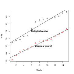
(a) Length of the stem

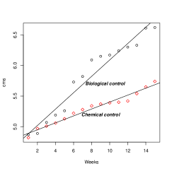
(b) Diameter of the floral button

Figure 1: Observations and adjusted values

Given that $R=2$, we can easily check graphically the conclusions reached in the hypothesis testing. Figure 1 (b) shows the intersection of lines for the floral button diameters, which explains the rejection of parallelism hypothesis. However, Figure 1(a) shows parallel lines, which certainly implies that the average length of stem for each sample per week is the same for both pest control. Similarly, Figure 1(a) depicts very different intercepts associated to the length of the stem, explaining the rejecting of the hypothesis for equal intercepts. Also, Figure 1(b) shows equal intercepts, which implies that the average floral button diameter for each sample in week zero is the same for both pest control.

The thesis Preciado-Ramírez (2014) concludes that the biological control method reduces infestation of the pest and as a consequence both the stem length and the button size are increased. This aspect promotes a higher sale price, but this result was not incorporated in the addressed work. Our analysis confirms these conclusions, but in a robust way that include all the variables simultaneously.

5 Conclusions

As a consequence of Subsection 3.1 the three hypotheses testing of this paper are valid under the complete family of elliptically contoured distribution, i.e. in any practical circumstance we can assume that our information have a matrix multivariate elliptically contoured distribution instead of considering the usual non realistic normality.

References

- Draper and Smith (1981) N. R. Draper and H. Smith, Applied regression analysis, 2nd edition. Wiley, New York, 1981.
- Fang and Zhang (1990) K. T. Fang and Y. T. Zhang, Generalized Multivariate Analysis, Science Press, Springer-Verlag, Beijing, 1990.
- Graybill (1976) F. A. Graybill, Theory and Application of the Linear Model, Wadsworth & Brooks/Cole, Advances Books and Softwere, Pacific Grove, California, 1976.
- Gupta and Varga (1993) A. K. Gupta and T. Varga, Elliptically Contoured Models in Statistics, Kluwer Academic Publishers, Dordrecht, 1993.
- Kres (1983) H. Kres, Statistical Tables for Multivariate Analysis, Springer-Verlag, New York, 1983.
- Morrison (2003) D. F. Morrison, Multivariate Sattistical Methods, 4th Revision Edition Duxbury Advances Series, London, 2003.
- Muirhead (2005) R. J. Muirhead, Aspects of Multivariate Statistical Theory, John Wiley & Sons, New York, 2005.
- Preciado-Ramírez (2014) M. R. Preciado-Ramírez, Validation of Phytoseiulus persimilis Athias-Henriot and Neoseiulus californicus for control of Tetranychus urticae Koch in the cultivation of roses in greenhouses. Thesis of Agronomical Engineering. University of Guanajuato. Irapuato, Guanajuato, Mexico, 2014. (In Spanish.)
- Press (1982) S. J. Press, Applied Multivariate Analysis: Using Bayesian and Frequentist Methods of Inference, Second Edition, Robert E. Krieger Publishing Company, Malabar, FL, 1982.
- Rencher (1995) A. C. Rencher, Methods of Multivariate Analysis, John Wiley & Sons, New York, 1995.
- Roy (1957) S. N. Roy, Some Aspect of Multivariate Analysis, John Wiley & Sons, New York, 1957.
- Seber (1984) G. A. F. Seber, Multivariate Observations. John Wiley & Sons, New York, 1984.
- Srivastava and Khatri (1979) M. S. Srivastava, and C. G. Khatri, An Introduction to Multivariate Analysis. North-Holland Publ., Amsterdam, 1979.