Multi-user Beam-Alignment
for Millimeter-Wave Networks

Abstract

Millimeter-wave communications is the most promising technology for next-generation cellular wireless systems, thanks to the large bandwidth available compared to sub-6 GHz networks. Nevertheless, communication at these frequencies requires narrow beams via massive MIMO and beamforming to overcome the strong signal attenuation, and thus precise beam-alignment between transmitter and receiver is needed. The resulting signaling overhead may become a severe impairment, especially in mobile networks with high users density. Therefore, it is imperative to optimize the beam-alignment protocol to minimize the signaling overhead. In this paper, the design of energy efficient joint beam-alignment protocols for two users is addressed, with the goal to minimize the power consumption during data transmission, subject to rate constraints for both users, under analog beamforming constraints. It is proved that a bisection search algorithm is optimal. Additionally, the optimal scheduling strategy of the two users in the data communication phase is optimized based on the outcome of beam-alignment, according to a time division multiplexing scheme. The numerical results show significant decrease in the power consumption for the proposed joint beam-alignment scheme compared to exhaustive search and a single-user beam-alignment scheme taking place separately for each user.

I Introduction

Mobile data traffic has shown a tremendous growth in the past few decades, and is expected to increase by $53\%$ in each year until 2020 [1]. Traditionally, mobile data traffic is served almost exclusively by wireless systems operating under $6$ GHz, due to the availability of low-cost hardware and favorable propagation characteristics at these frequencies. However, conventional sub-$6$ GHz networks cannot support the high data rate required by applications such as high definition video streaming, due to limited bandwidth availability. For this reason, millimeter-wave (mm-wave) systems operating between $30$ to $300$ GHz are receiving growing interest in both 5G related research and industry [2],[3].

The large bandwidth available in the mm-wave frequency band can better address the demands of the ever increasing mobile traffic. However, signal propagation at these frequencies is more challenging than traditional sub-6 GHz systems, due to factors such as high propagation loss, directivity, sensitivity to blockage [4], which are exacerbated with the increase in the carrier frequency. These features open up many challenges in both physical and MAC layers for the mm-wave frequencies to support high data rate. To overcome the propagation loss, mm-wave systems are expected to leverage narrow beam communication, via large-dimensional antenna arrays with directional beamforming at both base stations (BSs) and mobile users (MUs), as well as signal processing techniques such as precoding and combining [5].

Maintaining beam-alignment between transmitter and receiver is a challenging task in mm-wave networks, especially in dense and mobile networks: under high user density and mobility, frequent blockages and loss of alignment may occur, requiring frequent realignment. Unfortunately, the beam-alignment protocol may consume time, frequency and energy resources, thus potentially offsetting the benefits of mm-wave directionality. Motivated by this fact, in our previous work [6] we derived the optimal beam-width for communication, number of sweeping beams, and transmission energy so as to maximize the average rate under an average power constraint in a mobile scenario with a single user. Several schemes have been proposed to achieve beam-alignment in mm-wave networks. One of the most popular ones is exhaustive search, where the BS and the MU sequentially search through all possible combinations of transmit and receive beam patterns [7]. An iterative search algorithm is proposed in [8], where the BS first searches in wider sectors by using wider beams, and then refines the search within the best sector. In [9], we derived a throughput-optimal search scheme called bisection search, which refines search within the previous best sector by using a beam with half the width of the previous best sector. It is shown that the bisection scheme outperforms both iterative and exhaustive schemes in terms of maximizing throughput in the communication phase. All these works focus on a single-user scenario and do not investigate how to exploit the beam-alignment protocols jointly across multiple users.

In the literature, multiuser mm-wave systems have been studied under the topic of precoding [10], [11], beamforming [12] and for wideband mm-wave systems, where the channel is characterized by multi-path components, different delays, Angle-of-Arrivals/Angle-of-Departures (AoAs/AoDs), and Doppler shifts [13]. In all of the previous work, the authors proposed new algorithms in order to enhance the system performance. However, the optimality with respect to optimizing the communication performance in multi-user settings is not established. All of these algorithms cost in terms of time and energy resources, and have a large effect on the directionality achieved in the data communication phase, and thus on power consumption and achievable rate. This motivates us to seek how to optimally balance resources among beam-alignment and data communication.

In this paper, we consider the optimization of beam-alignment and data communication in a two-users mm-wave network. The BS transmits a sequence of beam-alignment beacons using a sequence of beams with different beam-shape, and refines its estimate on the position of the two users based on the feedback received. Afterwards, it schedules data transmission to the two users via time-division. Using a Markov decision process (MDP) formulation [14], we prove the optimality of a bisection search scheme during beam-alignment, which scans half of the uncertainty region associated to each user in each beam-alignment slot. We demonstrate numerically power savings up to $3\mathrm{dB}$ lower than under exhaustive search.

The rest of the paper is organized as follows. In Section II, we present the system model and the problem formulation, followed by the analysis in Section III. Numerical results are presented in Section IV, followed by concluding remarks in Section V. The proofs of the main analytical results are provided in the Appendix.

II System Model

We consider a mm-wave cellular network with a single base station (BS) and $M$ mobile users (MU_i), where $i{=}1,2,\cdots,M$, depicted in Fig. 1. In this paper, we consider the case $M{=}2$, and leave the more general case $M{\geq}2$ for future work.

The BS is located at the origin and the mobile user MU_i is located at angular coordinate $\Theta_{i}$, at distance $d_{i}$ from the BS, where $\Theta_{i}\in[0,2\pi]$ and $d_{i}\leq d_{\max}$, with $d_{\max}>0$ being the coverage area of the BS. We assume that $\Theta_{i}$ is uniformly distributed in $[\frac{-\sigma}{2},\frac{\sigma}{2}]$, denoted as $\Theta_{i}\sim\mathcal{U}[\frac{-\sigma}{2},\frac{\sigma}{2}]$ where $\sigma\in(0,2\pi]$ represents the availability of prior information on the angular coordinate of MU_i. We assume a single signal path between the BS and each MU, either line-of-sight (LOS) or a strong non-LOS signal (e.g., when the LOS signal is temporarily obstructed due to mobility).

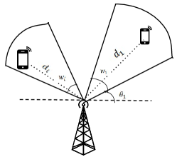
Figure 1: Beam pattern for multiuser system model.

The BS uses analog beamforming with a single RF chain. Data transmission is orthogonalized across users. We model the transmission beam of the BS using a generalization of the sectored antenna model [15]: the overall transmission beam is the superposition of multiple beams, each covering a specific sector, which can be implemented via phase shifters [16]. In addition, we ignore the effect of secondary beam lobes. Thus, we represent the beam shape (part of our design) at time $k$ via the set $\mathcal{B}_{k}\subseteq[-\pi,\pi]$, which represents the set of angular directions covered by the transmission beam. Furthermore, we assume that the MUs receive isotropically. The proposed analysis can be extended to non-isotropic MUs by using multiple beam-alignment stages, each corresponding to a specific beam pattern at the MU [17].

We assume a frame-slotted network with frame duration $T_{\mathrm{fr}}$ [s]. Each frame is divided into a beam-alignment phase of duration $T_{\mathrm{BA}}$ (Sec. II-A), followed by a data communication phase of duration $T_{\mathrm{cm}}{=}T_{\mathrm{fr}}{-}T_{\mathrm{BA}}$ (Sec. II-B), shown in Fig. 2.

II-A Beam-Alignment Phase

In this section, we describe the beam-alignment phase, executed in the initial portion of the frame, of duration $T_{\mathrm{BA}}$. Beam-alignment is performed over $L$ slots, each of duration $T\triangleq T_{\mathrm{BA}}/L$. As shown in Fig 2, at the beginning of each slot $k=0,1,\dots,L-1$, the BS sends a beacon $b_{k}$ of duration $T_{b}<T$, using a beam with beam-shape $\mathcal{B}_{k}$, and receives a feedback message from both MUs in the remaining portion $T-T_{b}$ of the slot.

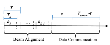
Figure 2: Timing diagram of the beam-alignment and data communication phases.

The beam-shape $\mathcal{B}_{k}$ is designed based on the current probability density function (PDF) of MUs’ angles $(\Theta_{1},\Theta_{2})$, denoted as $S_{k}(\theta_{1},\theta_{2})$, which is updated via Bayes’ rule based on the feedback received from both MUs, see (5). We also let $S_{k,1}(\theta_{1})=\int_{-\pi}^{\pi}S_{k}(\theta_{1},\theta_{2})\mathrm{d}\theta_{2}$ and $S_{k,2}(\theta_{2})=\int_{-\pi}^{\pi}S_{k}(\theta_{1},\theta_{2})\mathrm{d}\theta_{1}$ be the marginal PDF of MU₁ and MU₂, respectively. Note that, at time $0$, $\Theta_{i}\sim\mathcal{U}[\frac{-\sigma}{2},\frac{\sigma}{2}]$, hence

$$S_{0,1}(\theta)=S_{0,2}(\theta)=\frac{1}{\sigma}\chi\left(\theta\in\left[\frac{-\sigma}{2},\frac{\sigma}{2}\right]\right),$$ (1)

$$S_{0}(\theta_{1},\theta_{2})=S_{0,1}(\theta_{1})\cdot S_{0,2}(\theta_{2}),$$ (2)

where $\chi(.)$ is the indicator function. For convenience, we define the support of $S_{k,i}$ as

$$\mathcal{S}_{k,i}\triangleq\mathrm{supp}(S_{k,i}),$$ (3)

which defines the region of uncertainty for MU_i at time $k$.

If MU_i is located within $\mathcal{B}_{k}$, i.e., $\Theta_{i}\in\mathcal{B}_{k}$, then it detects the beacon signal successfully and it transmits an acknowledgment (ACK) back to the BS, denoted as $c_{i,k}{=}1$. Otherwise, it sends a negative-ACK (NACK), denoted as $c_{i,k}{=}0$, to inform the BS that no beacon has been detected. We assume that the feedback message $c_{i,k}\in\{0,1\}$ is received without error by the BS, within the end of the slot. This can be accomplished over a reliable low-frequency control channel, which does not require directional transmission and reception [18]. Additionally, we assume that the beacon is detected with no false-alarm nor mis-detection errors. This assumption requires a dedicated beam design to achieve small error probabilities [19]. Thus, we can express the feedback signal as

$$C_{k,i}=\chi(\Theta_{i}\in\mathcal{B}_{k}).$$ (4)

Given the sequence of feedback signals $C^{k}\triangleq(c_{0,1},c_{0,2}\cdots c_{k,1},c_{k,2})$ received up to slot $k$, and the sequence of beam shapes $\mathcal{B}^{k}\triangleq(\mathcal{B}_{0},\cdots,\mathcal{B}_{k})$ used for beam-alignment, the BS updates the PDF on the MUs’ angular coordinate based on Bayes’ rule as

$$S_{k+1}(\theta_{1},\theta_{2})=f(\theta_{1},\theta_{2}\mid\mathcal{B}^{k},C^{k-1},c_{k,1},c_{k,2})$$ (5)

$$\!\!\overset{(a)}{=}\frac{\mathbb{P}(c_{k,1},c_{k,2}\mid\theta_{1},\theta_{2},\mathcal{B}^{k},C^{k-1})f(\theta_{1},\theta_{2}\mid\mathcal{B}^{k},C^{k-1})}{\int_{[-\pi,\pi]^{2}}\mathbb{P}(c_{k,1},c_{k,2}\mid\tilde{\bm{\theta}},\mathcal{B}^{k},C^{k-1})f(\tilde{\bm{\theta}}\mid\mathcal{B}^{k},C^{k-1})\mathrm{d}\tilde{\bm{\theta}}}$$

$$\!\!\overset{(b)}{=}\frac{\mathbb{P}(c_{k,1}\mid\theta_{1},\mathcal{B}_{k})\mathbb{P}(c_{k,2}\mid\theta_{2},\mathcal{B}_{k})S_{k}(\theta_{1},\theta_{2})}{\int_{-\pi}^{\pi}\int_{-\pi}^{\pi}\mathbb{P}(c_{k,1}\mid\tilde{\theta}_{1},\mathcal{B}_{k})\mathbb{P}(c_{k,2}\mid\tilde{\theta}_{2},\mathcal{B}_{k})S_{k}(\tilde{\theta}_{1},\tilde{\theta}_{2})\mathrm{d}\tilde{\theta}_{1}\mathrm{d}\tilde{\theta}_{2}},$$

where $f(\cdot|\cdot)$ denotes conditional PDF. In step $(a)$, we applied Bayes’ rule; in step $(b)$, we used the previous PDF $f(\theta_{1},\theta_{2}|\mathcal{B}^{k},C^{k-1}_{i})=S_{k}(\theta_{1},\theta_{2})$ and the fact that $c_{k,i}$ is a function of $\Theta_{i}$ and $\mathcal{B}_{k}$ via (4).

II-B Communication Phase

In the communication phase of duration $T_{\mathrm{cm}}$, the BS schedules the two MUs using time division multiplexing (TDM). Specifically, it transmits to MU₁ over a portion $\tau_{1}\leq T_{\mathrm{cm}}$ of the data communication interval, using the transmission power $P_{L,1}$ and beam with shape $\mathcal{B}_{L,1}$, and to MU₂ over the remaining interval of duration $T_{\mathrm{cm}}-\tau_{1}$, with power $P_{L,2}$ and using a beam with shape $\mathcal{B}_{L,2}$.

The powers $P_{L,i}$ and beam-shapes $\mathcal{B}_{L,i}$ for both MUs, and the time allocation $\tau_{1}$ are designed based on the PDF of the MUs’ angular direction $S_{L}$ at the beginning of the communication phase, so as to support the rate $R_{i}$ over the entire frame. The beam-shape $\mathcal{B}_{L,i}$ for MU_i is chosen so as to provide coverage to guarantee successful transmission, i.e.,

$$\mathcal{B}_{L,i}=\mathcal{S}_{L,i}.$$ (6)

Thus, we can express the rate $R_{i}$ [bps/Hz] for both MUs as

$$R_{1}=\frac{\tau_{1}}{T_{\mathrm{fr}}}\log_{2}\left(1+\gamma_{1}\frac{P_{L,1}}{\omega_{L,1}}\right),$$ (7)

$$R_{2}=\frac{T_{\mathrm{cm}}-\tau_{1}}{T_{\mathrm{fr}}}\log_{2}\left(1+\gamma_{2}\frac{P_{L,2}}{\omega_{L,2}}\right),$$ (8)

where $\gamma_{i}\equiv\frac{\lambda^{2}d_{i}^{-\alpha}}{8\pi N_{0}W_{\mathrm{tot}}}$ is the SNR scaling factor, $\alpha$ is the path loss exponent, $N_{0}$ is the noise power spectral density, $W_{\mathrm{tot}}$ is the total bandwidth and $\omega_{L,i}\triangleq|\mathcal{B}_{L,i}|$ is the overall beam-width of the transmission beam. These equations presume that the transmission power $P_{L,i}$ is spread evenly across the transmit directions defined by the beam shape $\mathcal{B}_{L,i}$, so that the received SNR is $\gamma_{i}P_{L,i}/\omega_{L,i}$. We then express the energy expenditure as a function of the rate requirements as

$$E_{1}\triangleq\tau_{1}P_{L,1}=\omega_{L,1}\epsilon_{1}\left(\tau_{1}\right),$$ (9)

$$E_{2}\triangleq(T_{\mathrm{cm}}-\tau_{1})P_{L,2}=\omega_{L,2}\epsilon_{2}(T_{\mathrm{cm}}-\tau_{1}),$$ (10)

where we have defined

$$\epsilon_{i}(\tau)\triangleq\tau\frac{2^{\frac{T_{\mathrm{fr}}}{\tau}R_{i}}-1}{\gamma_{i}}$$ (11)

as the energy per radian required to transmit with average rate $R_{i}$ to MU_i over an interval of duration $\tau$.

III Optimization and Analysis

We define a policy $\pi$ as a function that, given the PDF $S_{k}$, selects the beam-shape $\mathcal{B}_{k}$ in each beam-alignment slot $k=0,1,\dots,L-1$, the power $P_{L,i}$, beam-shape $\mathcal{B}_{L,i}$ and time allocation $\tau_{1},T_{\mathrm{cm}}-\tau_{1}$ for both MUs during the data communication interval. The goal is to design $\pi$ so as to minimize the average power consumption in the data communication phase, with rate constraints $R_{1}$ and $R_{2}$ for both MUs. This optimization problem is expressed as

$$\bar{P}_{\mathrm{avg}}\triangleq\underset{\pi}{\text{min}}\ \mathbb{E}_{\mu}\Big{[}\frac{\omega_{L,1}}{T_{\mathrm{fr}}}\epsilon_{1}\left(\tau_{1}\right)+\frac{\omega_{L,2}}{T_{\mathrm{fr}}}\epsilon_{2}\left(T_{\mathrm{cm}}-\tau_{1}\right)\Big{]},$$ (12)

where the expectation is with respect to the beam-shapes and time allocation prescribed by policy $\pi$, and the angular coordinates of the MUs. We neglect the energy consumption in the beam-alignment phase, studied in [20] for the single-user case, and thus assume that data communication is the most energy-hungry operation.

III-A Markov Decision Process formulation

We formulate the optimization problem as a MDP, with state given by the PDF of the angular coordinates of the two MUs, $S_{k}$ in slots $k=0,1,\dots,L$. During the beam-alignment phase, policy $\pi$ dictates the beam-shape in slot $k$ as

$$\mathcal{B}_{k}=\pi_{k}(S_{k}).$$ (13)

At the end of the beam-alignment phase, the BS selects the time allocation $\tau_{1}$ for MU₁ and $T_{\mathrm{cm}}-\tau_{1}$ for MU₂ to be used during the communication phase. As explained previously, the beam-shape is chosen via (6) to provide coverage, and the power $P_{L,i}$ via (7)-(8) to support the rate demands. Thus, policy $\pi$ dictates the time allocation as

$$\tau_{1}=\pi_{L}(S_{L}).$$ (14)

Given the PDF $S_{k}$ and the beam-shape $\mathcal{B}_{k}$ during the beam-alignment slots, the MUs generate the feedback $(C_{k,1},C_{k,2})$ via (4), with probability distribution

$$\mathbb{P}\left(\left.C_{k,1}{=}c_{1},C_{k,2}{=}c_{2}\right|S_{k},\mathcal{B}_{k}\right)=\!\!\!\!\!\!\!\int\limits_{\mathcal{B}_{k}^{c_{1}}\times\mathcal{B}_{k}^{c_{2}}}\!\!\!\!\!S_{k}(\theta_{1},\theta_{2})\mathrm{d}\theta_{1}\mathrm{d}\theta_{2},$$ (15)

where we have defined the set operation

$$\mathcal{A}^{1}\equiv\mathcal{A},\ \mathcal{A}^{0}\equiv[0,2\pi]\setminus\mathcal{A}.$$ (16)

Optimizating $\pi$ is challenging due to the continuous PDF space. We now prove some structural properties of the model, which allow to simplify the state space.

Theorem 1.

We have that

$$S_{k}(\theta_{1},\theta_{2})=S_{k,1}(\theta_{1})\cdot S_{k,2}(\theta_{2}) \!\!\!\!\!\!\text{(independence)},$$ (17)

$$S_{k,i}(\theta_{i})=\frac{1}{|\mathcal{S}_{k,i}|}\chi(\theta_{i}\in\mathcal{S}_{k,i}) \!\!\!\!\!\!\text{(uniform distribution)}.$$ (18)

Moreover, either $\mathcal{S}_{k,1}\equiv\mathcal{S}_{k,2}$ or $\mathcal{S}_{k,1}\cap\mathcal{S}_{k,2}\equiv\emptyset$.

Proof.

See Appendix A. ∎

The independence and uniform distribution expressed by Theorem 1 imply that the feedback signals generated by the two MUs are statistically independent of each other, i.e., $\mathbb{P}\left(\left.C_{k,1}=c_{1},C_{k,2}=c_{2}\right|S_{k},\mathcal{B}_{k}\right)=\mathbb{P}\left(\left.C_{k,1}=c_{1}\right|S_{k,1},\mathcal{B}_{k}\right)\mathbb{P}\left(\left.C_{k,1}=c_{1}\right|S_{k,2},\mathcal{B}_{k}\right),$ with the probability of ACK given by

$$\mathbb{P}\left(\left.C_{k,i}=1\right|S_{k,i},\mathcal{B}_{k}\right)=\frac{|\mathcal{B}_{k}\cap\mathcal{S}_{k,i}|}{|\mathcal{S}_{k,i}|},$$ (19)

since $\Theta_{i}$ is uniformly distributed in the support $\mathcal{S}_{k,i}$. The next state $S_{k+1}$ is then a deterministic function of the PDF $S_{k}$, beam-shape $\mathcal{B}_{k}$ and feedback $(c_{k,1},c_{k,2})$ via Bayes’ rule, as in (5), and the support $\mathcal{S}_{k+1,i}$ for each MU is given by

$$\mathcal{S}_{k+1,i}\equiv\mathcal{S}_{k,i}\cap\mathcal{B}_{k}^{C_{k,i}},\ \forall i\in\{1,2\}.$$ (20)

We define the uncertainty width for MU_i as $U_{k,i}\triangleq|\mathcal{S}_{k,i}|$. Note that, the larger $U_{k,i}$, the more the uncertainty on the angular coordinate of MU_i. Additionally, let $\rho_{k}\triangleq\chi(\mathcal{S}_{k,1}\equiv\mathcal{S}_{k,2})$ be the binary variable indicating whether $\mathcal{S}_{k,1}\equiv\mathcal{S}_{k,2}$ (the two MUs are within the same uncertainty region, $\rho_{k}=1$) or $\mathcal{S}_{k,1}\cap\mathcal{S}_{k,2}\equiv\emptyset$ (the two MUs are in different uncertainty regions, $\rho_{k}=0$). We also define $\omega_{i}\triangleq|\mathcal{S}_{k,i}\cap\mathcal{B}_{k}|$ as the beam-width within the uncertainty region of MU_i. Note that, if $\rho_{k}=1$, then it follows that $\mathcal{S}_{k,1}\equiv\mathcal{S}_{k,2}$, hence $\omega_{k,1}=\omega_{k,2}$. We have the following result.

Theorem 2.

$(U_{k,1},U_{k,2},\rho_{k})$ is a sufficient statistic to select $(\omega_{1},\omega_{2})$ at time $k$. Given $(\omega_{1},\omega_{2})$, the beam-shape $\mathcal{B}_{k}$ may be arbitrary provided that $|\mathcal{S}_{k,i}\cap\mathcal{B}_{k}|=\omega_{i},\forall i\in\{1,2\}$.

Proof.

See Appendix B. ∎

Therefore, in the following we can focus on the design of the beam-widths $(\omega_{1},\omega_{2})$. With this notation, the probability of ACK can be written as

$$\mathbb{P}\left(\left.C_{k,i}=1\right|U_{k,i},\omega_{k,i}\right)=\frac{\omega_{k,i}}{U_{k,i}}.$$ (21)

Thus, given the state $(U_{k,1},U_{k,2},\rho_{k})$ in slot $k=0,1,\dots,L{-}1$ and the beam-widths $(\omega_{k,1},\omega_{k,2})$, the new state becomes $(U_{k+1,1},U_{k+1,2},\rho_{k+1})$ where

$$U_{k+1,i}=\left\{\begin{array}[]{ll}|\mathcal{B}_{k}\cap\mathcal{S}_{k,i}|=\omega_{k,i}&C_{k,i}=1,\\ |\mathcal{B}_{k}^{0}\cap\mathcal{S}_{k,i}|=U_{k,i}-\omega_{k,i}&C_{k,i}=0,\end{array}\right.$$ (24)

and

$$\rho_{k+1}=\left\{\begin{array}[]{ll}\rho_{k}&c_{k,1}=c_{k,2},\\ 0&c_{k,1}\neq c_{k,2},\end{array}\right.$$ (27)

with probabilities given by (21). The rule (24) expresses the fact that, if an ACK is received, then the support of $S_{k+1,i}$ becomes $\mathcal{S}_{k+1,i}\equiv\mathcal{S}_{k,i}\cap\mathcal{B}_{k}$ as given by (20), with width $\omega_{k,i}=|\mathcal{S}_{k+1,i}|$. In contrast, if a NACK is received, then MU_i is located in the complement region $\mathcal{S}_{k+1,i}\equiv\mathcal{S}_{k,i}\setminus\mathcal{B}_{k}$, with width $U_{k,i}-\omega_{k,i}$. Rule (27) describes the evolution of $\rho_{k}$. When $\rho_{k}=0$, the two MUs are located in disjoint uncertainty regions. In the next slot, they will still be in disjoint regions, irrespective of the feedback received at the BS. In contrast, when $\rho_{k}=1$, if the MUs send discordant feedback signals ($C_{k,1}\neq C_{k,2}$), the BS infers that they are located in disjoint uncertainty regions, hence $\rho_{k+1}=0$; if the MUs send concordant feedback signals ($C_{k,1}=C_{k,2}$), the BS infers that they are still in the same uncertainty region, hence $\rho_{k+1}=1$. The optimal beam-alignment algorithm and MU scheduling can be found via dynamic programming (DP). At the beginning of the communication phase, given the state $(U_{L,1},U_{L,2},\rho_{L})$ the optimal time allocation $\tau_{1}$ is the minimizer of (see (12) and (6) with $\omega_{L,i}=|\mathcal{B}_{L,i}|=|\mathcal{S}_{L,i}|=U_{L,i}$)

$$\!\!\!\!V_{L}\!(U_{L,1},\!U_{L,2},\!\rho_{L})\!=\!\!\!\!\!\min_{\tau_{1}\in(0,T_{\mathrm{cm}})}\!\!\!\!U_{L,1}\epsilon_{1}\!\left(\tau_{1}\right)\!{+}U_{L,2}\epsilon_{2}\!\left(T_{\mathrm{cm}}\!{-}\tau_{1}\right)\!.\!\!$$ (28)

Note that the objective function is convex in $\tau_{1}\in(0,T_{\mathrm{cm}})$, and it diverges for $\tau_{1}\to 0$ and $\tau_{1}\to T_{\mathrm{cm}}$. Thus, the optimal $\tau_{1}^{*}$ is the unique solver of

$$\frac{\epsilon_{2}^{\prime}\left(T_{\mathrm{cm}}-\tau_{1}^{*}\right)}{\epsilon_{1}^{\prime}\left(\tau_{1}^{*}\right)}=\frac{U_{L,1}}{U_{L,2}},$$ (29)

where $\epsilon_{i}^{\prime}(\tau)$ is the first order derivative of $\epsilon_{i}(\tau)$ with respect to $\tau$. The function $V_{L}(U_{L,1},U_{L,2},\rho_{L})$ denotes the cost-to-go function at the beginning of the communication phase. During the beam-alignment phase (slots $k=0,1,\dots,L-1$), the optimal value function for the cases $\rho_{k}=1$ and $\rho_{k}=0$ is computed recursively as

$$\!\!\!\!V_{k}(U,U,1){=}\!\!\!\min_{\omega\in[0,U]}\mathbb{E}\!\!\left[V_{k{+}1}(U_{k{+}1,1},U_{k{+}1,2},\rho_{k{+}1})\left|\!\!\begin{array}[]{l}\omega_{k,i}{=}\omega,\\ U_{k,i}{=}U,\\ \rho_{k}{=}1\end{array}\right.\!\!\!\right]$$ (33)

$$\!\!\!\!=\min_{\omega\in[0,U]}\frac{\omega^{2}}{U^{2}}V_{k+1}(\omega,\omega,1){+}\left(1{-}\frac{\omega}{U}\right)^{2}V_{k+1}(U{-}\omega,U{-}\omega,1)$$

$$+\frac{\omega}{U}\left(1{-}\frac{\omega}{U}\right)\bigr{[}V_{k+1}(\omega,U{-}\omega,0)+V_{k+1}(U{-}\omega,\omega,0)\bigr{]}$$ (34)

and

$$\!\!\!\!\!V_{k}(U_{1},U_{2},0){=}\!\!\!\min_{\omega_{i}\in[0,U_{i}]}\!\!\!\!\mathbb{E}\!\!\left[\!V_{k+1}(U_{k+1,1},U_{k+1,2},\rho_{k+1})\!\!\left|\!\!\begin{array}[]{l}\omega_{k,i}{=}\omega_{i},\\ U_{k,i}{=}U_{i},\\ \rho_{k}{=}0\end{array}\right.\!\!\!\!\!\right]$$ (38)

$$=\min_{\omega\in[0,U_{k}]}\frac{\omega_{1}}{U_{1}}\frac{\omega_{2}}{U_{2}}V_{k+1}(\omega_{1},\omega_{2},0)$$

$$+\frac{\omega_{1}}{U_{1}}\left(1{-}\frac{\omega_{2}}{U_{2}}\right)V_{k+1}(\omega_{1},U_{2}{-}\omega_{2},0)$$

$$+\left(1{-}\frac{\omega_{1}}{U_{1}}\right)\frac{\omega_{2}}{U_{2}}V_{k+1}(U_{1}{-}\omega_{1},\omega_{2},0)$$

$$+\left(1-\frac{\omega_{1}}{U_{1}}\right)\left(1-\frac{\omega_{2}}{U_{2}}\right)V_{k+1}(U_{1}-\omega_{1},U_{2}-\omega_{2},0).$$ (39)

These expressions are obtained by computing the expectation of $V_{k+1}(U_{k+1,1},U_{k+1,2},\rho_{k+1})$, with respect to the realization of the feedback signals $(C_{k,1},C_{k,2})$, with distribution (21), and the state dynamics given by (24) and (27).

In the next theorem, we prove the optimality of a bisection beam-alignment algorithm, which selects the beam-widths as $\omega_{k,i}=U_{k,i}/2$ in each slot.

Theorem 3.

The optimal beam-widths during the beam-alignment phase are given by

$$\omega_{k,i}=\frac{1}{2}U_{k,i}.$$ (40)

Then,

$$\bar{P}_{\mathrm{avg}}=\frac{\sigma}{T_{\mathrm{fr}}2^{L}}\Big{[}\epsilon_{1}\left(\tau_{1}^{*}\right)+\epsilon_{2}\left(T_{\mathrm{cm}}-\tau_{1}^{*}\right)\Big{]},$$ (41)

where $\tau_{1}^{*}$ uniquely satisfies

$$\frac{\epsilon_{2}^{\prime}\left(T_{\mathrm{cm}}-\tau_{1}^{*}\right)}{\epsilon_{1}^{\prime}\left(\tau_{1}^{*}\right)}=1.$$ (42)

Proof.

See Appendix C. ∎

Note that, in the special case $\gamma_{1}=\gamma_{2}=\gamma$, (42) yields

$$\tau_{1}^{*}=\frac{R_{1}}{R_{1}+R_{2}}T_{\mathrm{cm}}$$ (43)

and

$$\bar{P}_{\mathrm{avg}}=\frac{\sigma}{\gamma 2^{L}}\frac{T_{\mathrm{cm}}}{T_{\mathrm{fr}}}\left(2^{\frac{T_{\mathrm{fr}}}{T_{\mathrm{cm}}}(R_{1}+R_{2})}-1\right).$$ (44)

IV Numerical Results

In this section, we compare the total power consumption versus the sum rate $R_{\mathrm{tot}}=R_{1}+R_{2}$ under:

• The proposed joint beam-alignment bisection algorithm.

• Single-user beam-alignment [9]: in this scheme, odd frames are allocated to MU₁ using $L_{1}$ slots for beam-alignment, even frames to MU₂ using $L_{2}$ slots for beam-alignment. Beam-alignment is executed using the bisection scheme, whose optimality has been proved in [9] for the single user scheme. To achieve the target rate demand $R_{i}$ over a period of two frames, the rate demand for MU_i is set to $2\times R_{i}$ in the corresponding allocated frame.

• Joint exhaustive search: the BS scans exhaustively up to $K=2^{L}$ beams, each with beam-width $2\pi/K$, starting from beam index $1$ to beam index $K$. When both MUs are detected, the communication phase starts, using the TDM scheme described in Section II-B. If MU_i is located in the beam with index $\mathrm{id}_{i}$, beam-alignment will take $\max\{\mathrm{id}_{1},\mathrm{id}_{2}\}$ slots, followed by data communication over the remaining interval $T_{\mathrm{fr}}-\max\{\mathrm{id}_{1},\mathrm{id}_{2}\}T$.

The parameters $L$, $L_{1}$, $L_{2}$ are optimized to achieve the minimum power consumption, constrained to $L,L_{1},L_{2}\leq 7$. Thus, the minimum beam resolution is given by $2\pi/128$.

We consider this scenario: $T_{\mathrm{fr}}=2\mathrm{ms}$, $\sigma=2\pi$, $T=10\mu\mathrm{s}$, $d_{i}=50\mathrm{m}$, $W_{tot}=500\mathrm{MHz}$, $\lambda=5\mathrm{mm}$ (carrier frequency $60\mathrm{GHz}$), $\alpha=2$, $N_{0}=-174\mathrm{dBm}$. It follows that $\gamma_{1}=\gamma_{2}$. We vary $R_{1}$ and let $R_{2}=\psi R_{1}$, for a fixed parameter $\psi\in[0,1]$.

The results are plotted in Fig. 3. We notice that, when the rate for both MUs are equal ($\psi=1$), both joint and single-user beam-alignment have the same performance. We note that the power consumption under the joint beam-alignment scheme with bisection is independent of $\psi$, but only depends on the sum rate, as can be seen in (44). Using a similar argument as to derive (44), the same holds under joint exhaustive search. In contrast, the power consumption under single-user beam-alignment is highly affected by $\psi$. This is due to the fact that an entire frame is allocated to MU₂, despite its rate demand is only a fraction $\psi$ of that of MU₁. This causes great imbalances in the power allocated to the two MUs (such imbalance disappears when $\psi=1$, so that the rate demands are the same). Instead, with joint beam-alignment, the two MUs are scheduled optimally based on TDM, yielding significant power savings. We note that the joint beam-alignment scheme with bisection has the least power consumption, with $3\mathrm{dB}$ power saving compared to joint exhaustive search, and up to $7\mathrm{dB}$ compared to single-user beam-alignment, for moderate imbalances on the rate demands ($\psi=0.5$).

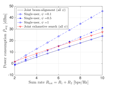
Figure 3: Power versus sum rate under different algorithms.

V Conclusions

In this paper, we studied the design of energy efficient joint beam-alignment protocols for two users, with the goal to minimize the power consumption during data transmission, subject to rate constraints for both users, under analog beamforming constraints. We prove that a bisection search algorithm is optimal. In addition we schedule optimally the two users during data communication via time division multiplexing, based on the outcome of beam-alignment. Our numerical results show significant power savings compared to exhaustive search and a single-user beam-alignment scheme taking place separately for each user.

Appendix A: Proof of Theorem 1

Note that (4) along with Bayes’ rule (5) imply (20). We prove the theorem by induction. The induction hypothesis holds for $k=0$, see (1). Now, assume that it holds in slot $k\geq 0$. We show that this implies that it holds in slot $k+1$ as well. Thus, assume that either $\mathcal{S}_{k,1}\equiv\mathcal{S}_{k,2}$ or $\mathcal{S}_{k,1}\cap\mathcal{S}_{k,2}\equiv\emptyset$. First, let us consider the case $\mathcal{S}_{k,1}\equiv\mathcal{S}_{k,2}$ with $C_{k,1}=C_{k,2}$. From (20) we have that

$$\mathcal{S}_{k+1,1}\equiv\mathcal{S}_{k,1}\cap\mathcal{B}_{k}^{C_{k,1}}\equiv\mathcal{S}_{k,2}\cap\mathcal{B}_{k}^{C_{k,2}}\equiv\mathcal{S}_{k+1,2},$$

and thus $\mathcal{S}_{k+1,1}\equiv\mathcal{S}_{k+1,2}$. For all other cases, we have that

$$\mathcal{S}_{k+1,1}\cap\mathcal{S}_{k+1,2}\equiv(\mathcal{S}_{k,1}\cap\mathcal{S}_{k,2})\cap(\mathcal{B}_{k}^{C_{k,1}}\cap\mathcal{B}_{k}^{C_{k,2}})\equiv\emptyset,$$

since either $\mathcal{S}_{k,1}\cap\mathcal{S}_{k,2}\equiv\emptyset$ from the induction hypothesis, or $\mathcal{S}_{k,1}\equiv\mathcal{S}_{k,2}$ but $C_{k,1}\neq C_{k,2}$, yielding $\mathcal{B}_{k}^{C_{k,1}}\cap\mathcal{B}_{k}^{C_{k,2}}\equiv\mathcal{B}_{k}^{0}\cap\mathcal{B}_{k}^{1}\equiv\emptyset$. Thus, it follows that either $\mathcal{S}_{k,1}\equiv\mathcal{S}_{k,2}$ or $\mathcal{S}_{k,1}\cap\mathcal{S}_{k,2}\equiv\emptyset$.

Now, assume that $S_{k}$ satisfies (17) and (18) in slot $k$. By specializing Bayes’ rule (5) to this case, we obtain

$$S_{k+1}(\theta_{1},\theta_{2})=\frac{\prod_{i\in\{1,2\}}\chi(\theta_{i}\in\mathcal{S}_{k,i}\cap\mathcal{B}_{k}^{c_{k,i}})}{\int_{-\pi}^{\pi}\int_{-\pi}^{\pi}\prod_{i\in\{1,2\}}\chi(\tilde{\theta}_{i}\in\mathcal{S}_{k,i}\cap\mathcal{B}_{k}^{c_{k,i}})\mathrm{d}\tilde{\theta}_{1}\mathrm{d}\tilde{\theta}_{2}},$$

where we have used (4) and (16), and the fact that $\chi(\theta_{i}\in\mathcal{B}_{k}^{c_{k,i}})\chi(\theta_{i}\in\mathcal{S}_{k,i})=\chi(\theta_{i}\in\mathcal{S}_{k,i}\cap\mathcal{B}_{k}^{c_{k,i}})$. Solving the integral in the denominator and using (20) we obtain

$$S_{k+1}(\theta_{1},\theta_{2})=\prod_{i\in\{1,2\}}\frac{1}{|\mathcal{S}_{k+1,i}|}\chi(\theta_{i}\in\mathcal{S}_{k+1,i}),$$

thus proving the induction step. The theorem is proved.

Appendix B: Proof of Theorem 2

We prove this theorem by induction. Let $V_{k}(S_{k})$ be the value function from state $S_{k}$ in slot $k$. At the beginning of the communication phase, from (12) we have that

$$V_{L}(S_{L})=\underset{\tau_{1}}{\text{min}}\ U_{L,1}\epsilon_{1}\left(\tau_{1}\right)+U_{L,2}\epsilon_{2}\left(T_{\mathrm{cm}}-\tau_{1}\right),$$ (45)

since the condition (6) implies $\omega_{L,i}=|\mathcal{B}_{L,i}|=|\mathcal{S}_{L,i}|=U_{L,i}$. Therefore,

$$V_{L}(S_{L})=V_{L}(|S_{L,1}|,|S_{L,2}|,\chi(S_{L,1}\equiv S_{L,2})).$$ (46)

Now, let $k<L$ and assume that $(U_{k+1,1},U_{k+1,2},\rho_{k+1})$ is a sufficient statistic to choose $\omega_{j,i}$ for $j\geq k+1$, with $\mathcal{B}_{j}$ such that $|\mathcal{S}_{j,i}\cap\mathcal{B}_{j}|=\omega_{j,i},\forall i\in\{1,2\}$, i.e.,

$$V_{k+1}(S_{k+1})=V_{k+1}(|S_{k+1,1}|,|S_{k+1,2}|,\chi(S_{k+1,1}\equiv S_{k+1,2})).$$

The dynamic programming iteration yields

$$V_{k}(S_{k})=\min_{\mathcal{B}_{k}}\mathbb{E}\left[V_{k+1}(S_{k+1})|\mathcal{B}_{k},\mathcal{S}_{k}\right]$$ (47)

$$\!{=}\min_{\mathcal{B}_{k}}\mathbb{E}\left[V_{k+1}(|S_{k+1,1}|,|S_{k+1,2}|,\chi(S_{k+1,1}{\equiv}S_{k+1,2}))|\mathcal{B}_{k},\mathcal{S}_{k}\right]\!\!,$$

where we have used the induction hypothesis.

Note that $\mathcal{S}_{k+1,i}$ is obtained via (20). If $\mathcal{S}_{k,1}\equiv\mathcal{S}_{k,2}$ ($\rho_{k}=1$), it follows that $\mathcal{S}_{k+1,1}\equiv\mathcal{S}_{k+1,2}$ ($\rho_{k+1}=1$) iff $C_{k,1}=C_{k,2}$, yielding $\rho_{k+1}=\chi(C_{k,1}=C_{k,2})$. If $\mathcal{S}_{k,1}\cap\mathcal{S}_{k,2}\equiv\emptyset$ ($\rho_{k}=1$), it follows that $\mathcal{S}_{k+1,1}\cap\mathcal{S}_{k+1,2}\equiv\emptyset$, hence $\rho_{k+1}=0$. Therefore, we can write

$$\rho_{k+1}=\rho_{k}\chi(C_{k,1}=C_{k,2}).$$ (48)

By computing the expectation with respect to the feedback distribution given by (19), and using (20), we then obtain

$$V_{k}(S_{k})=\min_{\mathcal{B}_{k}}\sum_{(c_{1},c_{2})\in\{0,1\}^{2}}\frac{|\mathcal{B}_{k}^{c_{1}}\cap\mathcal{S}_{k,1}|}{|\mathcal{S}_{k,1}|}\frac{|\mathcal{B}_{k}^{c_{2}}\cap\mathcal{S}_{k,2}|}{|\mathcal{S}_{k,2}|}$$

$$\times V_{k+1}(|\mathcal{S}_{k,1}\cap\mathcal{B}_{k}^{c_{1}}|,|\mathcal{S}_{k,2}\cap\mathcal{B}_{k}^{c_{2}}|,\rho_{k}\chi(c_{1}=c_{2}))).$$

Now, letting $\omega_{k,i}\triangleq|\mathcal{S}_{k,i}\cap\mathcal{B}_{k}|$ and $|\mathcal{S}_{k,i}|=U_{k,i}$, we find that $|\mathcal{S}_{k,i}\cap\mathcal{B}_{k}^{0}|=U_{k,i}-\omega_{k,i}$, yielding

$$V_{k}(S_{k})=\min_{\mathcal{B}_{k}}\sum_{(c_{1},c_{2})\in\{0,1\}^{2}}\prod_{i\in\{1,2\}}\frac{\omega_{k,i}^{c_{i}}(U_{k,i}-\omega_{k,i})^{1-c_{i}}}{U_{k,i}}\$$

$$\times V_{k+1}(\omega_{k,1}^{c_{1}}(U_{k,1}-\omega_{k,1})^{1-c_{1}},\omega_{k,2}^{c_{2}}(U_{k,2}-\omega_{k,2})^{1-c_{2}}$$

$$\qquad\qquad\qquad\qquad\qquad\qquad\qquad\qquad,\rho_{k}\chi(c_{1}=c_{2})).$$

Note that, given $(\omega_{k,1},\omega_{k,2})$ and $(U_{k,1},U_{k,2},\rho_{k})$, the objective function is independent of $\mathcal{B}_{k}$ and $S_{k}$. Thus, the minimization over $\mathcal{B}_{k}$ can be restricted to a minimization over $(\omega_{k,1},\omega_{k,2})$, with the additional constraint that $\omega_{k,1}=\omega_{k,2}$ if $\mathcal{S}_{k,1}\equiv\mathcal{S}_{k,2}$ ($\rho_{k}=0$), yielding

$$V_{k}(S_{k})=V_{k}(U_{k,1},U_{k,2},\rho_{k}).$$ (49)

The induction step is proved, hence the theorem.

Appendix C: Proof of Theorem 3

We prove the theorem by induction. In particular, we show that, for all $k=0,1,\dots,L$,

$$V_{k}(U_{1},U_{2},\rho)=V_{L}\left(\frac{U_{1}}{2^{L-k}},\frac{U_{2}}{2^{L-k}},0\right),\ \forall\rho\in\{0,1\}.$$ (50)

This condition clearly holds for $k=L$, since $V_{L}(U_{1},U_{2},\rho)=V_{L}\left(U_{1},U_{2},0\right)$ from (38). Thus, let $k<L$ and assume that

$$V_{k+1}(U_{1},U_{2},\rho)=V_{L}\left(\frac{U_{1}}{2^{L-k-1}},\frac{U_{2}}{2^{L-k-1}},0\right).$$ (51)

We prove that this implies (50). $V_{k}$ is computed from $V_{k+1}$ via DP, as in (33) and (38).

We start from the case $\rho_{k}=0$, and then consider the case $\rho_{k}=1$ (which implies $U_{k,1}=U_{k,2}$ and $\omega_{k,1}=\omega_{k,2}$). Let

$$g(x_{1},x_{2})\triangleq x_{1}x_{2}V_{k+1}(x_{1},x_{2},0).$$ (52)

Then, we can write the DP recursion (38) as

$$V_{k}(U_{1},U_{2},0)=\min_{\omega_{i}\in[0,U_{i}]}\frac{\frac{1}{2}g(\omega_{1},\omega_{2})+\frac{1}{2}g(U_{1}-\omega_{1},\omega_{2})}{U_{1}U_{2}/2}$$

$$+\frac{\frac{1}{2}g(\omega_{1},U_{2}-\omega_{2})+\frac{1}{2}g(U_{1}-\omega_{1},U_{2}-\omega_{2})}{U_{1}U_{2}/2}.$$ (53)

We denote the objective function in (Appendix C: Proof of Theorem 3) as $h(\omega_{1},\omega_{2})$, so that we can rewrite $V_{k}(U_{1},U_{2},0)=\min_{\omega_{i}\in[0,U_{i}]}h(\omega_{1},\omega_{2})$. In the final part of the proof, we will show that $g(x_{1},x_{2})$ is a convex function of $x_{i},i\in\{1,2\}$ (although not necessarily jointly convex with respect to $(x_{1},x_{2})$). By applying Jensen’s inequality to $h(\omega_{1},\omega_{2})$ in (Appendix C: Proof of Theorem 3), first with respect to the first argument of the function $g(\cdot,\cdot)$, and then with respect to the second argument, it follows that

$$h(\omega_{1},\omega_{2})\geq\frac{\frac{1}{2}g\left(\frac{U_{1}}{2},\omega_{2}\right)+\frac{1}{2}g\left(\frac{U_{1}}{2},U_{2}-\omega_{2}\right)}{U_{1}U_{2}/4}\geq\frac{g\left(\frac{U_{1}}{2},\frac{U_{2}}{2}\right)}{U_{1}U_{2}/4}.$$

Thus, it follows that

$$V_{k}(U_{1},U_{2},0)\geq 4\frac{g(U_{1}/2,U_{2}/2)}{U_{1}U_{2}}.$$ (54)

Indeed, it can be seen by inspection that such lower bound is achievable by the bisection policy $\omega_{i}=U_{i}/2$, which proves the induction step for the case $\rho_{k}=0$.

We now consider the case $\rho_{k}=1$. Using the fact that $V_{k+1}(U_{1},U_{2},0)=V_{k+1}(U_{1},U_{2},1)$ from the induction hypothesis, from (33) we obtain

$$V_{k}(U,U,1){=}\!\!\!\min_{\omega\in[0,U]}\mathbb{E}\!\!\left[V_{k{+}1}(U_{k{+}1,1},U_{k{+}1,2},0)\!\!\left|\!\!\begin{array}[]{l}\omega_{k,i}{=}\omega,\\ U_{k,i}{=}U,\\ \rho_{k}{=}1\end{array}\right.\!\!\!\right]$$ (58)

$$\geq\min_{(\omega_{1},\omega_{2})\in[0,U]^{2}}\mathbb{E}\!\!\left[V_{k{+}1}(U_{k{+}1,1},U_{k{+}1,2},0)\!\!\left|\!\!\begin{array}[]{l}\omega_{k,i}{=}\omega_{i},\\ U_{k,i}{=}U,\\ \rho_{k}{=}1\end{array}\right.\!\!\!\right]$$ (62)

$$=V_{k}(U,U,0),$$ (63)

where the inequality follows from the fact that we have extended the optimization interval to $(\omega_{1},\omega_{2})\in[0,U]^{2}$, and therefore $V_{k}(U,U,1)\geq V_{k}(U,U,0)$. We have seen that, for the case $\rho_{k}=0$, the value function is optimized by the bisection policy. By inspection, we can see that the lower bound $V_{k}(U,U,0)$ is also attained by the bisection policy $\omega_{k,1}=\omega_{k,2}=U/2$, which satisfies the requirement $\omega_{k,1}=\omega_{k,2}$ when $\rho_{k}=1$. Thus, we have proved the induction step.

By letting $k{=}0$ in (50) with $U_{1}{=}U_{2}{=}\sigma$, and using (28), we finally obtain (41) after dividing the energy consumption by the frame duration $T_{\mathrm{fr}}$. $\tau_{1}^{*}$ is the unique solution of (29), yielding (42) since $U_{L,i}=\sigma/2^{L}$ under bisection.

It remains to prove that $g(x_{1},x_{2})$ is a convex function of $x_{i},i\in\{1,2\}$. Due to the symmetry of $g(x_{1},x_{2})$ with respect to its arguments, it is sufficient to prove convexity with respect to $x_{1}$ only, with $x_{2}$ fixed. We have

$$g(x_{1},x_{2})=x_{1}x_{2}V_{L}\left(\frac{x_{1}}{2^{L-k-1}},\frac{x_{2}}{2^{L-k-1}},0\right)$$

$$=\frac{1}{2^{L-k-1}}\min_{\tau_{1}\in(0,T_{\mathrm{cm}})}x_{1}^{2}x_{2}\epsilon_{1}\left(\tau_{1}\right)+x_{1}x_{2}^{2}\epsilon_{2}\left(T_{\mathrm{cm}}-\tau_{1}\right).$$

Note that the convexity of $g(\cdot)$ is unaffected by $k$, thus we let $k=L-1$. Let $\tau_{1}(x_{1})$ be the minimizer above, as a function of $x_{1}$. We obtain

$$\frac{\mathrm{d}g(x_{1},x_{2})}{\mathrm{d}x_{1}}=2x_{1}x_{2}\epsilon_{1}\left(\tau_{1}(x_{1})\right)+x_{2}^{2}\epsilon_{2}\left(T_{\mathrm{cm}}-\tau_{1}(x_{1})\right)$$

$$+\tau_{1}^{\prime}(x_{1})x_{1}x_{2}\left[x_{1}\epsilon_{1}^{\prime}\left(\tau_{1}(x_{1})\right)-x_{2}\epsilon_{2}^{\prime}\left(T_{\mathrm{cm}}-\tau_{1}(x_{1})\right)\right],$$

where $\tau_{1}^{\prime}(x_{1})\triangleq\frac{\mathrm{d}\tau_{1}(x_{1})}{\mathrm{d}x_{1}}$. Note that $\tau_{1}(x_{1})$ must satisfy (29) (with $U_{L,i}=x_{i}$), yielding

$$\frac{\mathrm{d}g(x_{1},x_{2})}{\mathrm{d}x_{1}}=2x_{1}x_{2}\epsilon_{1}\left(\tau_{1}(x_{1})\right)+x_{2}^{2}\epsilon_{2}\left(T_{\mathrm{cm}}-\tau_{1}(x_{1})\right).$$

The second derivative of $g(x_{1},x_{2})$ with respect to $x_{1}$ is then given by

$$\frac{\mathrm{d}^{2}g(x_{1},x_{2})}{\mathrm{d}x_{1}^{2}}=2x_{2}\epsilon_{1}\left(\tau_{1}(x_{1})\right)+x_{1}x_{2}\epsilon_{1}^{\prime}\left(\tau_{1}(x_{1})\right)\tau_{1}^{\prime}(x_{1})$$

$$+\tau_{1}^{\prime}(x_{1})x_{2}\left[x_{1}\epsilon_{1}^{\prime}\left(\tau_{1}(x_{1})\right)-x_{2}\epsilon_{2}^{\prime}\left(T_{\mathrm{cm}}-\tau_{1}(x_{1})\right)\right].$$ (64)

Using again the fact that $\tau_{1}(x_{1})$ must satisfy (29), we obtain

$$\!\!\!\frac{\mathrm{d}^{2}g(x_{1},x_{2})}{\mathrm{d}x_{1}^{2}}=2x_{2}\epsilon_{1}\left(\tau_{1}(x_{1})\right){+}\epsilon_{1}^{\prime}\left(\tau_{1}(x_{1})\right)x_{1}x_{2}\tau_{1}^{\prime}(x_{1}).$$ (65)

From (29), we have that $\tau_{1}(x_{1})$ must satisfy $x_{2}\epsilon_{2}^{\prime}\left(T_{\mathrm{cm}}{-}\tau_{1}(x_{1})\right){=}x_{1}\epsilon_{1}^{\prime}\left(\tau_{1}(x_{1})\right)$. By computing the derivative with respect to $x_{1}$ on both sides of this equation, we obtain $\tau_{1}^{\prime}(x_{1})$ as

$$\tau_{1}^{\prime}(x_{1})=\frac{1}{x_{2}}\frac{[\epsilon_{1}^{\prime}\left(\tau_{1}(x_{1})\right)]^{2}}{\left[\begin{array}[]{l}-\epsilon_{1}^{\prime}\left(\tau_{1}(x_{1})\right)\epsilon_{2}^{\prime\prime}\left(T_{\mathrm{cm}}-\tau_{1}(x_{1})\right)\\ -\epsilon_{1}^{\prime\prime}\left(\tau_{1}(x_{1})\right)\epsilon_{2}^{\prime}\left(T_{\mathrm{cm}}-\tau_{1}(x_{1})\right)\end{array}\right]}.$$ (68)

Thus, by substituting in (65), the convexity of $g(x_{1},x_{2})$ ($\frac{\mathrm{d}^{2}g(x_{1},x_{2})}{\mathrm{d}x_{1}^{2}}>0$) becomes equivalent to

$$-2\epsilon_{1}\epsilon_{1}^{\prime}\epsilon_{2}^{\prime\prime}-2\epsilon_{1}\epsilon_{1}^{\prime\prime}\epsilon_{2}^{\prime}+\epsilon_{2}^{\prime}[\epsilon_{1}^{\prime}]^{2}>0$$ (69)

where $\epsilon_{i}$, $\epsilon_{i}^{\prime}$, $\epsilon_{i}^{\prime\prime}$ is shorthand notation for $\epsilon_{i}(\tau_{i}(x_{1}))$, $\epsilon_{i}^{\prime}(\tau_{i}(x_{1}))$, $\epsilon_{i}^{\prime\prime}(\tau_{i}(x_{1}))$, with $\tau_{2}(x_{1})=T_{\mathrm{cm}}-\tau_{1}(x_{1})$, respectively.

Let $y_{1}=\frac{T_{\mathrm{fr}}}{\tau_{1}}R_{1}$ and $y_{2}=\frac{T_{\mathrm{fr}}}{T_{\mathrm{cm}}-\tau_{1}}R_{2}$. We obtain

$$\left\{\begin{array}[]{l}\epsilon_{i}=\frac{2^{y_{i}}-1}{y_{i}}\frac{T_{\mathrm{fr}}R_{i}}{\gamma_{i}},\\ \epsilon_{i}^{\prime}=\frac{2^{y_{i}}-1}{\gamma_{i}}-\frac{2^{y_{i}}}{\gamma_{i}}\ln(2)y_{i},\\ \epsilon_{i}^{\prime\prime}=\frac{2^{y_{i}}}{\gamma_{i}T_{\mathrm{fr}}R_{i}}[\ln(2)]^{2}y_{i}^{3}.\end{array}\right.$$ (73)

Substituting in (69), convexity becomes equivalent to

$$q(y_{1},y_{2})\triangleq 2^{y_{2}}[\ln(2)y_{2}-1+2^{-y_{2}}]2[1-2^{-y_{1}}][\ln(2)]^{2}y_{1}^{2}$$

$$-2^{y_{2}}[\ln(2)y_{2}-1+2^{-y_{2}}][\ln(2)y_{1}-1+2^{-y_{1}}]^{2}$$ (74)

$$+2\frac{R_{1}}{R_{2}}[1-2^{-y_{1}}][\ln(2)y_{1}-1+2^{-y_{1}}][\ln(2)]^{2}\frac{2^{y_{2}}y_{2}^{3}}{y_{1}}>0,$$

which we are now going to prove. Using the fact that $\ln(2)y_{1}-1+2^{-y_{1}}>0$, we have that

$$q(y_{1},y_{2})\geq 2^{y_{2}}[\ln(2)y_{2}-1+2^{-y_{2}}]2[1-2^{-y_{1}}][\ln(2)]^{2}y_{1}^{2}$$

$$-2^{y_{2}}[\ln(2)y_{2}-1+2^{-y_{2}}][\ln(2)y_{1}-1+2^{-y_{1}}]^{2}$$ (75)

$$\propto 2[1-2^{-y_{1}}][\ln(2)]^{2}y_{1}^{2}-[\ln(2)y_{1}-1+2^{-y_{1}}]^{2}\triangleq\hat{q}(y_{1}),$$

where $\propto$ denotes proportionality up to the multiplicative positive factor $2^{y_{2}}[\ln(2)y_{2}-1+2^{-y_{2}}]>0$. The derivative of $\hat{q}(y_{1})$ with respect to $y_{1}$ is given by

$$\frac{\mathrm{d}\hat{q}(y_{1})}{\mathrm{d}y_{1}}=2\ln(2)[1-2^{-y_{1}}]^{2}$$

$$+2\ln(2)\ln(2)y_{1}[1-2^{-y_{1}}+2^{-y_{1}}\ln(2)y_{1}]>0.$$ (76)

Therefore, we obtain $q(y_{1},y_{2})\geq 2^{y_{2}}[\ln(2)y_{2}-1+2^{-y_{2}}]\hat{q}(y_{1})>2^{y_{2}}[\ln(2)y_{2}-1+2^{-y_{2}}]\hat{q}(0)=0$. The convexity of $g(x_{1},x_{2})$ with respect to $x_{i}$ is proved, hence the theorem.

References

- [1] C. Cisco, “Cisco visual networking index: Global mobile data traffic forecast update, 2014–2019 white paper,” Source:¡ http://www. cisco. com/c/en/us/solutions/collateral/service-provider/visual-networking-index-vni/white_paper_c11-520862. html, 2015.
- [2] Y. Niu, Y. Li, D. Jin, L. Su, and A. V. Vasilakos, “A survey of millimeter wave communications (mmwave) for 5g: opportunities and challenges,” Wireless Networks, vol. 21, no. 8, pp. 2657–2676, 2015.
- [3] T. S. Rappaport, R. W. Heath Jr, R. C. Daniels, and J. N. Murdock, Millimeter wave wireless communications. Pearson Education, 2014.
- [4] T. S. Rappaport et al., Wireless communications: principles and practice. prentice hall PTR New Jersey, 1996, vol. 2.
- [5] M. R. Akdeniz, Y. Liu, M. K. Samimi, S. Sun, S. Rangan, T. S. Rappaport, and E. Erkip, “Millimeter wave channel modeling and cellular capacity evaluation,” IEEE journal on selected areas in communications, vol. 32, no. 6, pp. 1164–1179, 2014.
- [6] N. Michelusi and M. Hussain, “Optimal beam sweeping and communication in mobile millimeter-wave networks,” ICC 2018, to appear, 2018.
- [7] C. Jeong, J. Park, and H. Yu, “Random access in millimeter-wave beamforming cellular networks: issues and approaches,” IEEE Communications Magazine, vol. 53, no. 1, pp. 180–185, 2015.
- [8] S. Hur, T. Kim, D. J. Love, J. V. Krogmeier, T. A. Thomas, A. Ghosh et al., “Millimeter wave beamforming for wireless backhaul and access in small cell networks.” IEEE Trans. Communications, vol. 61, no. 10, pp. 4391–4403, 2013.
- [9] M. Hussain and N. Michelusi, “Throughput optimal beam alignment in millimeter wave networks,” in Information Theory and Applications Workshop (ITA), 2017. IEEE, 2017, pp. 1–6.
- [10] A. Alkhateeb, G. Leus, and R. W. Heath, “Limited feedback hybrid precoding for multi-user millimeter wave systems,” IEEE transactions on wireless communications, vol. 14, no. 11, pp. 6481–6494, 2015.
- [11] A. Alkhateeb, R. W. Heath, and G. Leus, “Achievable rates of multi-user millimeter wave systems with hybrid precoding,” in Communication Workshop (ICCW), 2015 IEEE International Conference on. IEEE, 2015, pp. 1232–1237.
- [12] R. A. Stirling-Gallacher and M. S. Rahman, “Multi-user mimo strategies for a millimeter wave communication system using hybrid beam-forming,” in Communications (ICC), 2015 IEEE International Conference on. IEEE, 2015, pp. 2437–2443.
- [13] X. Song, S. Haghighatshoar, and G. Caire, “A robust time-domain beam alignment scheme for multi-user wideband mmwave systems,” arXiv preprint arXiv:1711.10954, 2017.
- [14] D. P. Bertsekas, D. P. Bertsekas, D. P. Bertsekas, and D. P. Bertsekas, Dynamic programming and optimal control. Athena scientific Belmont, MA, 1995, vol. 1, no. 2.
- [15] T. Bai and R. W. Heath, “Coverage and rate analysis for millimeter-wave cellular networks,” IEEE Transactions on Wireless Communications, vol. 14, no. 2, pp. 1100–1114, 2015.
- [16] O. Abari, H. Hassanieh, M. Rodriguez, and D. Katabi, “Millimeter wave communications: From point-to-point links to agile network connections,” in Proceedings of the 15th ACM Workshop on Hot Topics in Networks. ACM, 2016, pp. 169–175.
- [17] C. Jeong, J. Park, and H. Yu, “Random access in millimeter-wave beamforming cellular networks: issues and approaches,” IEEE Communications Magazine, vol. 53, no. 1, pp. 180–185, January 2015.
- [18] S. Rangan, T. S. Rappaport, and E. Erkip, “Millimeter-wave cellular wireless networks: Potentials and challenges,” Proceedings of the IEEE, vol. 102, no. 3, pp. 366–385, 2014.
- [19] M. Hussain, D. J. Love, and N. Michelusi, “Neyman-pearson codebook design for beam alignment in millimeter-wave networks,” in Proceedings of the 1st ACM Workshop on Millimeter-Wave Networks and Sensing Systems, ser. mmNets, vol. 17, 2017, pp. 17–22.
- [20] M. Hussain and N. Michelusi, “Energy Efficient Beam-Alignment in Millimeter Wave Networks,” Asilomar 2017.