A Unified Framework for Planning in
Adversarial and Cooperative Environments

Abstract

Users of AI systems may rely upon them to produce plans for achieving desired objectives. Such AI systems should be able to compute obfuscated plans whose execution in adversarial situations protects privacy, as well as legible plans which are easy for team members to understand in cooperative situations. We develop a unified framework that addresses these dual problems by computing plans with a desired level of comprehensibility from the point of view of a partially informed observer. For adversarial settings, our approach produces obfuscated plans with observations that are consistent with at least k goals from a set of decoy goals. By slightly varying our framework, we present an approach for goal legibility in cooperative settings which produces plans that achieve a goal while being consistent with at most j goals from a set of confounding goals. In addition, we show how the observability of the observer can be controlled to either obfuscate or clarify the next actions in a plan when the goal is known to the observer. We present theoretical results on the complexity analysis of our problems. We demonstrate the execution of obfuscated and legible plans in a cooking domain using a physical robot Fetch. We also provide an empirical evaluation to show the feasibility and usefulness of our approaches using IPC domains.

1 Introduction

AI systems have become quite ubiquitous. As users, we heavily rely on these systems to plan our day-to-day activities. Since all these systems have logging and tracking abilities, an observer can get access to our data and our actions. Such observers can be of two types: adversarial or cooperative. In adversarial settings, like mission planning, military intelligence, reconnaissance, counterintelligence, etc., protection of sensitive data can be of utmost importance to the agent. In such situations, it is necessary for an AI system to produce plans that reveal neither the intentions nor the activities of the agent. On the other hand, in case of a cooperative observer, the AI system should be able to produce plans that help clarify the intent of the agent. Therefore, it is desirable for an AI system to be capable of computing both obfuscated plans in adversarial settings and legible plans in cooperative settings.

In this work, we propose a new unifying formalization and algorithms for computing obfuscated plans as well as legible plans. In our framework, we consider two agents: an acting agent and an observer. The acting agent has full observability of its activities. The observer is aware of the agent’s planning model but has partial observability of the agent’s activities. The observations are emitted as a side effect of the agent’s activities and are received by the observer. In the following example, we illustrate the influence of an observation model on the belief space of the observer.

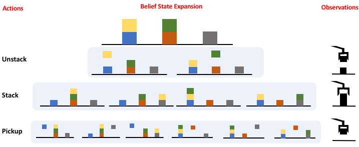
Figure 1: A blocksworld example illustrating belief expansion due to observation equivalence induced by the observation model of the observer.

Example 1.

Consider a blocksworld planning domain, where the actions unstack, stack, pickup and putdown are available. The observer can only receive partial observations using sensors on the table and on the gripper. An observation is emitted whenever the gripper is holding a block and indicates whether the block was lifted from the table or from the top of another block. This allows our observer to learn whether or not the current action has the agent holding a block (for example in unstack and pickup, it is holding a block) and whether or not the current action involves a block that was on the table (for example, in pickup and putdown, the blocks are picked up from / putdown on the table). Thus, our observer can distinguish between types of actions that were performed but is still unaware of which blocks were used. In Figure 1, we illustrate the progression of belief states from the observer’s point of view based on the observation model defined above.

An adversarial observer may be able to use the information gleaned from observations to interfere with or hamper the agent’s activities. For example, consider the keystroke timing attack (?) where the observer retrieves observations about keystroke timing by studying an agent’s inter-keystroke timings. Through such traffic analysis attacks, the observer can learn the passwords typed by an agent while connecting to a remote machine. On the other hand, in cooperative scenarios, an agent is required to communicate its intentions to the observer as quickly and clearly as possible. For example, consider a robot who is capable of assembling either chairs or tables. A chair has three components: seat, back and legs; and a table has two components: surface and legs. Whenever the robot is holding a component, the observer receives an observation regarding the type of component. In order to notify about a task of say, assembling a chair, the robot can start with the seat or the back components rather than with the legs to make its objectives clearer to the observer.

In this work, we develop a coherent set of notions for goal obfuscation and goal legibility. Our approach computes the solutions for each of these problems using the variants of a common underlying algorithm. Our approach assumes offline settings, where the observer receives the observations after the agent has finished executing a plan. In the case of a goal obfuscation problem, there exist multiple decoy goals and one true goal. The observer is unaware of the agent’s true goal, and the objective is to generate a plan solution without revealing it. Our solution ensures that at least $k$ goals are possible at the end of the observation sequence. On the other hand, in the goal legibility problem, there exist multiple confounding goals and a true goal. Here the objective is to reveal at most $j$ goals to the observer. Our solution ensures that at most $j$ goals are possible at the end of the observation sequence. We also consider a variant of obfuscation and legibility where the adversary knows the goal of the agent and wants to obfuscate or reveal the next action in the plan to achieve that goal, we call these problems plan obfuscation and plan legibility respectively. For plan obfuscation, the objective is to generate a plan solution with an observation sequence that is consistent with at least $\ell$ diverse plans. On the other hand, for plan legibility, the objective is to generate a plan solution that is consistent with at least $m$ similar plans.

In the following sections, we present a common framework that encapsulates the planning problems discussed above. And thereafter, we discuss each of the problems in detail. We also provide a theoretical and empirical analysis of the value and scope of our approaches.

2 Controlled Observability Planning Problem

2.1 Classical Planning

A classical planning problem can be defined as a tuple $\mathcal{P}=\langle\mathcal{F},\mathcal{A},\mathcal{I},G\rangle$, where $\mathcal{F}$, is a set of fluents, $\mathcal{A}$, is a set of actions. A state $s$ of the world is an instantiation, $\mathcal{F}^{i}$ of $\mathcal{F}$. The initial state $\mathcal{I}$ is the instantiation of all fluents in $\mathcal{F}$ and the goal $G$ is a subset of instantiated fluents in $\mathcal{F}$. Each action $a\in\mathcal{A}$ is a tuple of the form $\langle pre(a),add(a),delete(a),c(a)\rangle$ where $c(a)$ denotes the cost of an action, $pre(a)\subseteq\mathcal{F}$ is a set of preconditions for the action $a$, $add(a)\subseteq\mathcal{F}$ is a set of positive effects and $delete(a)\subseteq\mathcal{F}$ is a set of negative effects, i.e., $\Gamma(s,a)\models\bot$ if $s\not\models pre(a)$; else $\Gamma(s,a)\models s\cup add(a)\setminus delete(a)$ where $\Gamma(\cdot)$ is the transition function. The solution to $\mathcal{P}$ is a plan or a sequence of actions $\pi=\langle a_{1},a_{2},\ldots,a_{n}\rangle$, such that, $\Gamma(\mathcal{I},\pi)\models G$, i.e., starting from the initial state sequentially executing the actions lands the agent in a goal state. The cost of the plan, $c(\pi)$, is summation of the cost of all the actions in the plan $\pi$, $c(\pi)=\sum_{a_{i}\in\pi}c(a_{i})$.

2.2 Problem Setting

We now introduce a general planning problem framework that will be used to define adversarial and cooperative cases in the following sections. The controlled observability problem involves an acting agent and an observer.

Definition 1.

A controlled observability planning problem is a tuple, $\mathcal{P_{CO}}=\langle\mathcal{D},\mathcal{G},\Omega,\mathcal{O}\rangle$, where,

• $\mathcal{D}=\langle\mathcal{F},\mathcal{A},\mathcal{I}\rangle$ is the planning domain of the agent.

• $\mathcal{G}=\{G_{1}\cup G_{2}\ldots\cup G_{n-1}\cup G_{A}\}$ is a set of candidate goal conditions, each defined by subsets of fluent instantiations, where $G_{A}$ is the true goal of the agent.

• $\Omega=\{o_{i}|i=1,\ldots,m\}$ is a set of $m$ observations that can be emitted as a result of the action taken and the state transition.

• $\mathcal{O}:(\mathcal{A}\times\mathcal{S})\rightarrow\Omega$ is a many-to-one observation function which maps the action taken and the next state reached to an observation in $\Omega$. That is to say, the observations are deterministic, each $\langle a,s^{\prime}\rangle$ pair is associated with a single observation but multiple pairs can be mapped to the same observation.

The observer has access to $\mathcal{P_{CO}}$, but is unaware of the true goal of the agent. Also, the observer does not have access to the actions performed by the agent, instead receives the observations corresponding to the plan executed by the agent. The observation function can be seen as a sensor model, as modeled in several prior works (?; ?; ?). For every action taken by the agent and an associated state transition, the observer receives an observation. This observation might be consistent with multiple action-state pairs because of the many-to-one formulation of $\mathcal{O}$. Therefore, the observer operates in the belief space. The agent takes the belief space of the observer into account in its planning process, so as to control the observability of the observer. Our formulation defines an offline scenario where the observer receives all the observations once the plan has been executed by the agent.

2.3 Observer’s Belief Space

The observer may use its observations of the agent’s activity to maintain a belief state, or the set of possible states consistent with the observations.

Definition 2.

A belief, $b_{i}$, induced by observation, $o_{i}$, emitted by action, $a_{i}$, and resulting state, $s_{i}$, is, $b_{i}=\{\hat{s}_{i}~{}|~{}\exists\hat{a}_{i},\ \mathcal{O}(\hat{a}_{i},\hat{s}_{i})=o_{i}\land\mathcal{O}(a_{i},s_{i})=o_{i}\}$.

Whenever a new action is taken by the agent, the observer’s belief can be updated as follows:

Definition 3.

A belief update, $b_{i+1}$ for belief $b_{i}$ is defined as, $b_{i+1}=update(b_{i},o_{i+1})=\{\hat{s}_{i+1}~{}|~{}\exists\hat{s}_{i},\exists\hat{a}_{i+1},\ \Gamma(\hat{s}_{i},\hat{a}_{i+1})\models\hat{s}_{i+1}\land\hat{s}_{i}\in b_{i}\land\mathcal{O}(\hat{a}_{i+1},\hat{s}_{i+1})=o_{i+1}\}$.

A sequence of such belief updates gives us the observer’s belief sequence that is consistent with a sequence of observations emitted by the agent.

Definition 4.

A belief sequence induced by a plan p starting at state $s_{0}$, BS(p, $s_{0}$), is defined as a sequence of beliefs $\langle b_{o},b_{1},\ldots,b_{n}\rangle$ such that there exist $o_{0},o_{1},o_{2},\ldots,o_{n}\in\Omega$ where,

• $o_{i}=\mathcal{O}(a_{i},s_{i})$

• $b_{0}=\{\hat{s}_{0}|\mathcal{O}(\emptyset,s_{0})=o_{0}\land\mathcal{O}(\emptyset,\hat{s}_{0})=o_{0}\}$

• $b_{i+1}=update(b_{i},o_{i+1})$

The objective of the agent is to generate a desired belief in the observer’s belief space, such that the last belief in the induced belief sequence satisfies goal conditions from the candidate goal set $\mathcal{G}$ including $G_{A}$.

2.4 Variants of $\mathcal{P_{CO}}$

We now discuss the two major variants of $\mathcal{P_{CO}}$ namely, goal obfuscation and goal legibility planning problems.

Goal Obfuscation

The adversary is aware of agent’s candidate goal set but is unaware of agent’s true goal. The aim of goal obfuscation is to hide this true goal from the observer. This is done by taking actions towards agent’s true goal, such that, the corresponding observation sequence exploits the observer’s belief space in order to be consistent with multiple goals.

Definition 5.

A goal obfuscation planning problem, is a $\mathcal{P_{CO}}$, where, $\mathcal{G}=\{G_{A}\cup G_{1}\cup\ldots\cup G_{n-1}\}$, is the set of $n$ goals where $G_{A}$ is the true goal of the agent, and $G_{1},\ldots,G_{n-1}$ are decoy goals.

A solution to a goal obfuscation planning problem is a k-ambiguous plan. The objective here is to make the observation sequence consistent with at least $k$ goals, out of which $k-1$ are decoy goals, such that, $k\leq n$. These $k-1$ goals can be chosen by the robot so as to maximize the obfuscation.

Definition 6.

A plan, $\pi_{k}$, is a k-ambiguous plan, if $\Gamma(\mathcal{I},\pi_{k})\models G_{A}$ and the last belief, $b_{n}\in BS(\pi_{k},\mathcal{I})$, satisfies the following, $|b_{n}\cap\mathcal{G}|\geqslant k$, where $1\geqslant k\geqslant n$.

Definition 7.

An observation sequence $O_{k}=\langle o_{1},\ldots,o_{n}\rangle$ is k-ambiguous observation sequence if it is an observation sequence emitted by a k-ambiguous plan.

A k-ambiguous plan achieves at least $k$ goals in the last belief of the observation sequence.

Goal Legibility

The aim of goal legibility is to take goal-specific actions which help the observer in deducing the robot’s goal. This can be useful in cooperative scenarios where the robot wants to notify the observer about its goal without explicit communication. This case is exactly opposite of the obfuscation case.

Definition 8.

A goal legibility planning problem is a $\mathcal{P}_{CO}$, where, $\mathcal{G}=\{G_{A}\cup G_{1}\cup\ldots\cup G_{n-1}\}$ is the set of $n$ goals where $G_{A}$ is the true goal of the agent, and $G_{1},\ldots,G_{n-1}$ are confounding goals.

The objective here is to generate legible plans so as to reveal at most $j$ goals. Here we ensure that the plans are consistent with at most $j$ goals so as to minimize the number of goals in the observer’s belief space.

Definition 9.

A plan, $\pi_{j}$, is a j-legible plan, if $\Gamma(\mathcal{I},\pi_{j})\models G_{A}$ and the last belief, $b_{n}\in BS(\pi_{j},\mathcal{I})$, satisfies the following, $|b_{n}\cap\mathcal{G}|\leqslant j$, where $1\geqslant j\geqslant n$.

The definition of j-legible observation sequence follows that of k-ambiguous case.

2.5 Complexity Analysis

In this section, we discuss the complexity results for $\mathcal{P_{CO}}$. Given the Definitions 6 and 9 of goal obfuscation and goal legibility plan solutions, we prove that the plan existence problem for $\mathcal{P_{CO}}$ is EXPSPACE-complete.

Theorem 1.

The plan existence problem for a controlled observability planning problem is EXPSPACE-hard.

Proof.

To show that the plan existence problem for $\mathcal{P_{CO}}$ is EXPSPACE-hard, we will show that the NOD (No-Observability Deterministic) planning problem is reducible to $\mathcal{P_{CO}}$. The plan existence problem for NOD has been shown to be EXPSPACE-complete (?; ?).

Let $\mathcal{P}_{N}=\langle\mathcal{F}_{N},\mathcal{A}_{N},\mathcal{I}_{N},G_{N},\mathcal{V}\rangle$ be a NOD planning problem, where, $\mathcal{F}_{N}$ is the set of fluents (or Boolean state variables), such that, state $s$ is an instantiation of $\mathcal{F}_{N}$. $\mathcal{A}_{N}$ is a set of actions, such that, when an action $a\in\mathcal{A}_{N}$ is applied to a state, $s_{i}$, a deterministic transition to the next state occurs, $\Gamma(s_{i},a)\models s_{i+1}$. $\mathcal{I}$ and $G$ are Boolean formulae that represent sets of initial and goal states. $\mathcal{V}=\emptyset$ is the set of observable state variables. Since the underlying system state is unknown, the deterministic transition function does not reveal the hidden state. $\mathcal{P}_{N}$ can be expressed as a $\mathcal{P_{CO}}$ problem, $\mathcal{P}_{C}=\langle\mathcal{D}_{C},G_{C},\Omega_{C},\mathcal{O}_{C}\rangle$, where, $\mathcal{D}_{C}=\{\mathcal{F}_{C},\mathcal{A}_{C},\mathcal{I}_{C}\}$, such that $\mathcal{I}_{C}$ is a set of possible initial states, $G_{C}$ is a subset of instantiations in $\mathcal{F}_{C}$, $\Omega=\emptyset$ and $\mathcal{O}=\emptyset$.

Suppose $\pi_{\mathcal{P}_{C}}=\langle a_{1},\ldots,a_{r}\rangle$ is a plan solution to $\mathcal{P}_{C}$, such that, $\Gamma(\mathcal{I}_{C},\pi_{\mathcal{P}_{C}})\models G_{C}$ and the last belief $b_{r}\in BS(\pi_{\mathcal{P}_{C}},\mathcal{I}_{C})$ satisfies $|b_{r}\cap G_{C}|=1$. Then according to the definition of $\mathcal{P}_{N}$, the plan $\pi_{\mathcal{P}_{C}}$ has a last belief, such that, $\exists s_{r}\in b_{r},s_{r}\models G_{C}$ and therefore solves $\mathcal{P}_{N}$.

Conversely, suppose $\pi_{\mathcal{P}_{N}}=\langle a_{1},\ldots,a_{q}\rangle$ is a plan solution to $\mathcal{P}_{N}$, such that, $\Gamma(\mathcal{I}_{N},\pi_{\mathcal{P}_{N}})\models G_{N}$. Let $B_{q}$ be the belief associated with the last action in $\pi_{\mathcal{P}_{N}}$. Since it achieves the goal, we can say that $|B_{q}\cap G|=1$. According to Definitions 6, 9, for $k=j=1$, $B_{q}$ satisfies the condition. Therefore $\pi_{\mathcal{P}_{N}}$ is a solution to $\mathcal{P}_{C}$. ∎

Theorem 2.

The plan existence problem for a controlled observability planning problem is EXPSPACE-complete.

Proof.

In $\mathcal{P_{CO}}$, the planner operates in belief space and the state space is bounded by $2^{2^{|\mathcal{F}|}}$, where $|\mathcal{F}|$ is the cardinality of the fluents (or Boolean state variables). If there exists a plan solution for $\mathcal{P_{CO}}$, it must be bounded by $2^{2^{|\mathcal{F}|}}$ in length. Any solution longer in length must have loops, which can be removed. Therefore, by selecting actions non-deterministically, the solution can be found in at most $2^{2^{|\mathcal{F}|}}$ steps. Hence, the plan existence problem for $\mathcal{P_{CO}}$ is in NEXPSPACE. By Savitch’s theorem (?), NEXPSPACE = EXPSPACE. Therefore, the plan existence problem for $\mathcal{P_{CO}}$ is EXPSPACE-complete. ∎

2.6 Algorithm for Plan Computation

Input: $\mathcal{P_{CO}}=\langle\mathcal{D},\mathcal{G},\Omega,\mathcal{O}\rangle$

Output: plan solution $\pi_{\mathcal{P_{CO}}}$, observation sequence, $O_{\mathcal{P_{CO}}}$

1

2$\Delta\leftarrow 1$ $\triangleright$ Counter

3 $\Delta\_limit\leftarrow False$ $\triangleright$ Delta cardinality flag

4

5while $\Delta\leqslant|\mathcal{S}|$ do

6      

7      $s_{\Delta}\leftarrow\{\mathcal{I}\}$ $\triangleright$ Initial state

8       $open\leftarrow\texttt{Priority\_Queue()}$ $\triangleright$ Open list

9       $closed\leftarrow\{\}$ $\triangleright$ Closed list

10       $b_{0}\leftarrow\{\mathcal{O}(\emptyset,s_{\Delta})\}$ $\triangleright$ Initial belief

11       $open.push(\langle\mathcal{I},b_{0}\rangle,priority=0)$

12      

13      if $|s_{\Delta}|=\Delta$ then

14             $\Delta\_limit\leftarrow True$

15            

16       end if

17      

18      while $open\neq\emptyset$  do

19             $\langle s_{\Delta},b\rangle\leftarrow open.pop()$

20             if $\neg\Delta\_limit$ then

21                   for $\hat{s}\in b\setminus s_{\Delta}$  do

22                         $s_{\Delta}\leftarrow s_{\Delta}\cup\hat{s}$

23                         if $|s_{\Delta}|=\Delta$ then

24                               $\Delta\_limit\leftarrow True$

25                               break

26                         end if

27                        

28                   end for

29                  

30             end if

31            $closed\leftarrow closed\cup s_{\Delta}$

32             if  $\langle s_{\Delta},b\rangle\models$ GOAL-TEST($\mathcal{G}$) then

33                   $\textbf{return}~{}\pi_{\mathcal{P_{CO}}},O_{\mathcal{P_{CO}}}$

34             end if

35            

36            for $s_{\Delta}^{\prime}\in successors(s_{\Delta})$ do

37                   $o\leftarrow\mathcal{O}(a,s_{\Delta}^{\prime})$

38                   $b^{\prime}\leftarrow$ Belief-Generation($b,a,o$)

39                   $h(s_{\Delta}^{\prime})\leftarrow$ HEURISTIC-FUNCTION$(s_{\Delta}^{\prime},b^{\prime})$

40                   if $s_{\Delta}^{\prime}\notin$ open and $s_{\Delta}^{\prime}\notin$ closed then

41                         $open.push(\langle s_{\Delta}^{\prime},b^{\prime}\rangle,h(s_{\Delta}^{\prime}))$

42                        

43                   else if $h(s_{\Delta}^{\prime})<h^{prev}(s_{\Delta}^{\prime})$  then

44                         if $s_{\Delta}^{\prime}\notin$ open then

45                               $closed\leftarrow closed\setminus s_{\Delta}^{\prime}$

46                               $open.push(\langle s_{\Delta}^{\prime},b^{\prime}\rangle,h(s_{\Delta}^{\prime})$)

47                              

48                         else

49                               update priority from $h^{prev}(s_{\Delta}^{\prime})$ to $h(s_{\Delta}^{\prime})$

50                         end if

51                        

52                   end if

53                  

54             end for

55            

56       end while

57      $\Delta\leftarrow\Delta+1$

58       $\Delta\_limit\leftarrow False$

59      

60 end while

61

62procedure Belief-Generation($b$, $a$, $o$)

63 $b^{\prime}\leftarrow\{\}$

64 for $\hat{s}\in b$ do

65       for $\hat{a}\in\mathcal{A}$ do

66             if $\hat{s}\models pre(\hat{a})$ and $\mathcal{O}(\hat{a},\Gamma(\hat{s},\hat{a}))=o$ then

67                   $b^{\prime}\leftarrow b^{\prime}\cup\Gamma(\hat{s},\hat{a})$

68                  

69             end if

70            

71       end for

72      

73 end for

return $b^{\prime}$

Algorithm 1 Plan Computation

We present the details of a common algorithm template used by our formulations in Algorithm 1. In Section 3, we show how we customize the goal-test (line 1) and the heuristic function (line 1) to suit the needs of each of our problem variants. There are two loops in the algorithm: the outer loop (line 1) runs for different values of $\Delta=\{1,2,\ldots,|\mathcal{S}|\}$; while the inner loop (line 1) performs search over the state space of size ${|\mathcal{S}|\choose\Delta}$. These loops ensure the complete exploration of the belief space.

For each outer iteration, $s_{\Delta}$ is augmented with elements of the belief state until the cardinality of $s_{\Delta}$ is equal to the value of $\Delta$. In the inner loop, we run GBFS over the state space of $s_{\Delta}$. For each successor node in the open list, the belief induced by an observation is updated. The heuristic value of a state is computed using a plan graph (?) level based heuristic, such as set-level heuristic (?). The plan graph data structure contains information about the positive and the negative interactions between the sets of propositions and actions. We use set-level plan graph heuristic to guide the search. To get the set-level cost, the plan graph is populated with a state, $s$ (search node), and it is expanded until one of the following holds $\bf{(1)}$ the goal is reachable, that is, the goal propositions are present in a proposition layer and are mutex-free pairs, or $\bf{(2)}$ the graph levels off, that is, it cannot be expanded further. If the goal is not reachable before the graph levels off then it cannot be achieved by any plan. In this case, the heuristic cost is $\infty$. Else, when the goal is reachable and the goal propositions are pairwise mutex-free, the heuristic value is the index of the first plan graph layer that contains it.

Proposition 1.

Algorithm 1 necessarily terminates in finite number of $|\mathcal{S}|$ iterations, such that, the following conditions hold:

(Completeness) Algorithm 1 explores the complete solution space of $\mathcal{P_{CO}}$, that is, if there exists a $\pi_{\mathcal{P_{CO}}}$ that correctly solves $\mathcal{P_{CO}}$, it will be found.

(Soundness) The plan, $\pi_{\mathcal{P_{CO}}}$, found by Algorithm 1 correctly solves $\mathcal{P_{CO}}$ as ensured by the corresponding goal-test.

Algorithm 1 terminates either when a plan is found or after running the outer loop for $|\mathcal{S}|$ iterations. The outer loop ensures that the all the paths in the search space are explored. And the goal tests of both of the problem variants ensure that the solutions are correct with respect to Definitions 6 and 9.

The increase in cardinality of $s_{\Delta}$ can lead to increase in the search overhead. In our implementation, we run only the first iteration of the outer loop. Most of the problem instances can be solved in the first iteration itself.

3 Plan Computation

In this section, we present instantiations of modules presented in Algorithm 1 for goal obfuscation and legibility.

3.1 Computing Goal Obfuscated Plans

Goal test

We ensure that the solution plan does not end unless all $k$ goals occur in the belief state. In order to achieve this, the goal condition checks whether the goal has been achieved in the agent’s true state and also whether the $k-1$ goals have been achieved in the belief state. If there doesn’t exist a plan that can achieve the true goal with the given $k-1$ goals, we restart the search with next combination of $k-1$ goals among the total $n-1$ decoy goals.

Heuristic function

We now propose a heuristic strategy for generating a plan where the last belief state satisfies k goals, making it a k-ambiguous plan. We use two heuristic functions to estimate a node’s cost:

$$h(s)=\left(\textit{set-level}_{G_{A}}(s)+\textit{set-level}_{\mathcal{G}_{k-1}}(b)\right)$$ (1)

where the first heuristic computes the setLevel distance to the true goal from the agent’s actual state, while the second heuristic computes the setLevel distance to $k-1$ goals from the belief induced by the emitted observation. This is computed by finding the max of the minimum set-level distance from belief to each of the $k-1$ goals. The heuristic value of a state is computed as the total of these two values. The heuristic ensures at least $k$ goals occur in the last belief induced by the plan.

Note on deterministic output and use of noop

The k-ambiguous algorithm maintains obfuscation assuming that the adversarial observer does not have access to the process of plan computation. If the observer has access to it then, a simple variation like the addition of random noise to the heuristic can thwart the attack.

Our formulation supports the use of noops for obfuscation. A noop action can be compiled to multiple noop actions, $noop=\{pretend_{o_{i}}|i=1,\ldots,|\Omega|\}$ where each noop corresponds to an observation of a prior action. This would allow the agent to emit observations without doing any action. This way the agent can increase the chances of obfuscation while using the same approaches.

3.2 Computing Goal Legible Plans

Goal test

In this case, we have to ensure that the computed plan is consistent with at most $j$ true goals. To that end, we change our goal condition to additionally check whether at most $j-1$ confounding goals have been achieved in the last belief in $BS$, and whether at least $n-j$ goals are absent in the belief.

Heuristic function

In this case, our objective is to avoid at least $n-j$ goals and at the same time be consistent with at most $j$ goals. We achieve this by minimizing the set-level distance to true goal from the agent’s actual state and to the $j-1$ confounding goals from the agent’s belief state. However, we maximize the set-level distance to other $n-j$ goals in order to achieve at most $j$ goals. This is written as,

$$h(s)=\left(\textit{set-level}_{G_{A}}(s)+\textit{set-level}_{\mathcal{G}_{j-1}}(b)-\textit{set-level}_{\mathcal{G}_{n-j}}(b)\right)$$ (2)

4 Plan Obfuscation and Plan Legibility

We also discuss two other problem variants called plan obfuscation and plan legibility. These problems come into picture when the observer is aware of the agent’s goal. However, the objective here is to either obfuscate or reveal the next steps in the plan.

4.1 Obfuscation

We achieve plan obfuscation by computing a plan whose observation sequence conforms to a set of diverse plans, making it hard to predict the next action in that plan.

Definition 10.

A plan obfuscation planning problem is a tuple, $\mathcal{P}_{PO}=\langle\mathcal{D},\mathcal{G}_{PO},\Omega,\mathcal{O}\rangle$, where, $\mathcal{G}_{PO}=\{G_{A}\}$, and $G_{A}$ is the true goal of the agent.

The solution to a plan obfuscation planning problem is an $\ell$-diverse plan. An $\ell$-diverse plan has an observation sequence that is consistent with $\ell$ plans that are at least $d$ distance away. In order to compute an $\ell$-diverse plan, we need to keep track of the paths that are consistent with the belief sequence of the given plan, we call the set of these paths as belief plan set.

Definition 11.

A belief plan set, BPS(p, $s_{0}$) = $\{p_{1},\ldots,p_{n}\}$, induced by a plan $p$ starting at $s_{0}$, is a set of plans that are formed by causally consistent chaining of state sequences in $BS(p,s_{0})$, i.e., BPS(p, $s_{0}$) = $\{\langle\hat{s}_{0},\hat{a}_{1},\hat{s}_{1},\ldots,\hat{s}_{n}\rangle~{}|~{}\exists~{}\hat{a}_{j},~{}\hat{s}_{j-1}\models pre(\hat{a}_{j})~{}\wedge~{}\hat{s}_{j-1}\in b_{j-1}~{}\wedge~{}\hat{s}_{j}\models\hat{s}_{j-1}\cup add(\hat{a}_{j})\setminus delete(\hat{a}_{j})~{}\wedge~{}\hat{s}_{j}\in b_{j}\}$.

Our aim is to compute the diversity between all the pairs of plans in $BPS(p,s_{0})$. The diversity between plans can be enforced by using plan distance measures.

Plan Distance Measures

We will utilize the three plan distance measures introduced in ? (?), and refined in ? (?), namely action, causal link and state sequence distances. Our aim is to use these plan distance measures to measure the diversity of plans in a belief plan set.

Action distance

We denote the set of unique actions in a plan $\pi$ as $A(\pi)=\{a~{}|~{}a\in\pi\}$. Given the action sets $A(p_{1})$ and $A(p_{2})$ of two plans $p_{1}$ and $p_{2}$ respectively, the action distance is, $\delta_{A}(p_{1},p_{2})=1-\frac{\lvert A(p_{1})\cap A(p_{2})\rvert}{\lvert A(p_{1})\cup A(p_{2})\rvert}$.

Causal link distance

A causal link represents a tuple of the form $\langle a_{i},p_{i},a_{i+1}\rangle$, where $p_{i}$ is a predicate that is produced as an effect of action $a_{i}$ and used as a precondition for $a_{i+1}$. The causal link distance for the causal link sets $Cl(p_{1})$ and $Cl(p_{2})$ of plans $p_{1}$ and $p_{2}$ is, $\delta_{C}(p_{1},p_{2})=1-\frac{\lvert Cl(p_{1})\cap Cl(p_{2})\rvert}{\lvert Cl(p_{1})\cup Cl(p_{2})\rvert}$.

State sequence distance

This distance measure takes the sequences of the states into consideration. Given two state sequence sets $S(p_{1})=(s^{p_{1}}_{0},\ldots,s^{p_{1}}_{n})$ and $S(p_{2})=(s^{p_{2}}_{0},\ldots,s^{p_{3}}_{n^{\prime}})$ for $p_{1}$ and $p_{2}$ respectively, where $n\geq n^{\prime}$ are the lengths of the plans, the state sequence distance is, $\delta_{S}(p_{1},p_{2})=\frac{1}{n}\big{[}\ \sum_{k=1}^{n^{\prime}}d(s_{k}^{p_{1}},s_{k}^{p_{2}})+n-n^{\prime}\big{]}\ \$, where $d(s_{k}^{p_{1}},s_{k}^{p_{2}})=1-\frac{\lvert s_{k}^{p_{1}}\cap s_{k}^{p_{2}}\rvert}{\lvert s_{k}^{p_{1}}\cup s_{k}^{p_{2}}\rvert}$ represents the distance between two states (where $s_{k}^{p_{1}}$ is overloaded to denote the set of fluents in state $s_{k}^{p_{1}}$).

We now formally define $\ell$-diverse plan and other terms.

Definition 12.

Two plans, $p_{1},p_{2}$, are a d-distant pair with respect to distance function $\delta$ if, $\delta(p_{1},p_{2})=d$, where $\delta$ is a diversity measure.

Definition 13.

A BPS induced by plan p starting at $s_{0}$ is minimally d-distant, $d_{min}(BPS(p,s_{0}))$, if $\displaystyle d=\min_{p1,p2\in BPS(p,s_{0})}\delta(p1,p2)$.

Definition 14.

A plan, $\pi_{l}$, is an $\bm{\ell}$-diverse plan, if for a given value of d and distance function $\delta$, $d_{min}(BPS(\pi_{l},\mathcal{I}))\geq d$, $|BPS(\pi_{l},\mathcal{I})|\geq\ell$, where $\ell\geq 2$ and every plan in $BPS(\pi_{l},\mathcal{I})$ achieves the goal in $\mathcal{G}_{PO}$.

Computing Obfuscated Plans

Here we return a plan that is at least $\ell$-diverse and that maximizes the plan distance between BPS induced by a plan.

Goal test

To ensure the plans in $BPS$ induced by $\ell$-diverse plan can achieve the goal in $\mathcal{G_{PO}}$, we change the goal condition to additionally check whether at least $\ell$ plans are reaching the goal or not. Also in order to ensure termination of the algorithm, there is a cost-bound given as input to the algorithm.

Heuristic function

We now present our heuristic strategy to compute $\ell$-diverse observation sequence. Our heuristic is a three-part function:

$$h(s)=\left(-d_{min}(BPS(p,s_{0})),-|BPS(p,s_{0})|,\textit{set-level}(s)\right)$$ (3)

where the primary heuristic maximizes the $d$ of $d_{min}(BPS(p,s_{0}))$ induced by plan $p$ starting at $s_{0}$, the second heuristic maximizes the cardinality of the set $BPS(p,s_{0})$, while the third heuristic gives the set-level value of $s$. The cardinality of $BPS(p,s_{0})$ is computed by counting the number of plans that have the same set-level value from their last states as that from the true state. The distance is computed using either of the three plan distances.

4.2 Plan Legibility

The definition of plan legibility planning problem is similar to that of plan obfuscation planning problem. Here the objective is to reveal the next action in the plan. We achieve this by making the observation sequence consistent with plans that are similar in terms of observation sequences. This case is opposite to that of the plan obfuscation case. We use the same three plan distance measures to define the similarity of the plans. We call the solution to this problem as an m-similar plan. For similar plans in $BPS$, we define the maximum distance between any two pairs of plans.

Definition 15.

A BPS induced by plan p starting at $s_{0}$ is maximally d-distant, $d_{max}(BPS(p,s_{0}))$, if $d=\displaystyle\max_{p1,p2\in BPS(p,s_{0})}\delta(p1,p2)$.

Definition 16.

A plan, $\pi_{m}$, is a m-similar plan, if for a given value of d and distance function $\delta$, $d_{max}(BPS(\pi_{m},\mathcal{I}))\leq d$, $|BPS(\pi_{m},\mathcal{I})|\geq m$, where $m\geq 2$ and every plan in $BPS(\pi_{m},\mathcal{I})$ achieves the goal in $\mathcal{G}_{PL}$.

Computing Legible Plans

Here we return a plan that is at least $m$-similar and that minimizes the plan distance between BPS induced by a plan. The goal test for this case is similar to that of plan obfuscation case.

Heuristic function

The heuristic function to compute $m$-similar observation sequence is a three-part function:

$$h(s)=\left(d_{max}(BPS(p,s_{0})),-|BPS(p,s_{0})|,\textit{set-level}(s)\right)$$ (4)

where the primary heuristic minimizes the $d$ value of $d_{max}(BPS(p,s_{0}))$ induced by plan $p$ starting at $s_{0}$, the remaining parts are same as those in plan obfuscation case.

5 Robot Demonstration

We now present a demonstration of k-ambiguity and j-legibility using a physical Fetch robot in a cooking domain. Here robot plays the role of an actor and a human plays the role of an observer. The goal of the robot is to add necessary ingredients to make a recipe. In the obfuscation setting, the robot’s aim is to hide the ingredients from the human. This can be of use, especially, in scenarios where there is a need to preserve the secrecy of a recipe due to proprietary reasons. In contrast, in the legibility setting, the robot’s aim is to inform the human about the ingredients being added. This could be seen from a household user’s perspective, where the user needs to know what is being used in the recipe.

The domain consists of actions that allow the robot to communicate with the human, as well as pick-up and pour ingredients into a container. Each action can be performed in either an obfuscated or a legible way with different effects and different observations. We provide the action descriptions in Figures 3 and 4. From Figure 3, it can be seen that the action ask-human-to-stir distracts the human and allows the robot to obfuscate its goal. When the human is inattentive, the observation emitted for picking up any ingredient is generic. On the other hand, in Figure 4 the action ask-human-to-pass-sugar brings the human to attention. When the human is attentive, the observation emitted for picking up a container is specific for each ingredient. As shown in Figure 2, the scenario consists of a salt container and two sugar containers: one labeled as sugar, another without a label. The human is not aware of the contents of the unlabeled container.

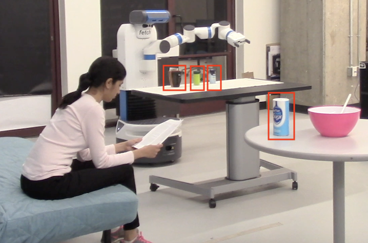
Figure 2: An illustration of the cooking domain. Here the robot is following a recipe and has to pick up and pour the ingredients into a cup. The robot has two containers available on its table, an unlabeled green colored container that contains sugar (unbeknownst to the human) and a labeled salt container. A labeled sugar container is available on the second table.

(:action ask-human-to-stir

:parameters (?x - ingredient ?y - container)

:precondition (and

(in ?x ?y)

(not (obfuscated ?y))

)

:effect (and

(human-inattentive)

(increase (total-cost) 1)

)

)

(:action pickup-container-obfuscated

:parameters (?x - ingredient ?y - container

?z - table)

:precondition (and

(in ?x ?y)

(handempty)

(on ?y ?z)

(accessible ?z)

(human-inattentive)

)

:effect (and

(not (handempty))

(holding ?y)

(not (on ?y ?z))

(obfuscated ?y)

(increase (total-cost) 1)

)

)

Figure 3: Action description of obfuscating actions

(:action ask-human-to-pass-sugar

:parameters (?x - ingredient ?y - container

?z - table)

:precondition (and

(in ?x ?y)

(is-type-labeled ?y)

(accessible ?z)

(not (legible ?y))

)

:effect (and

(on ?y ?z)

(human-attentive)

(increase (total-cost) 1)

)

)

(:action pickup-container-legible

:parameters (?x - ingredient ?y - container

?z - table)

:precondition (and

(in ?x ?y)

(handempty)

(on ?y ?z)

(accessible ?z)

(is-type-labeled ?y)

(human-attentive)

)

:effect (and

(not (handempty))

(holding ?y)

(not (on ?y ?z))

(legible ?y)

(increase (total-cost) 1)

)

)

Figure 4: Action description of legible actions

We used MoveIt (?) software with RRTConnectkConfigDefault planner to perform motion planning. RViz was used to visualize the objects in the scene and the possible trajectories of the robot. AR markers were used to localize the objects in the scene. The candidate goal set along with k-ambiguous and j-legible plans are given in Table 1. Here $k=2$ and $j=1$. The videos for both obfuscation and legibility can be viewed at https://youtu.be/mW7qCeggpUA and https://youtu.be/qzvTivKuszU.

Table 1: Obfuscated and legible plans for cooking domain

True Goal	contents-added cup1 sugar
Decoy / Confounding	contents-added cup1 salt
Obfuscated Plan	ask-human-to-stir sugar container1,
	pickup-container-obfuscated sugar container1 table1,
	pour-ingredient-and-place sugar container1 cup1 table1
Obfuscation observation	human-inattentive, pickup-ingredient, pour-ingredient
Legible Plan	ask-human-to-pass-sugar sugar container2 table1,
	pickup-container-legible sugar container2 table1,
	pour-ingredient-and-place sugar container2 cup1 table1
Legible observation	human-attentive, pickup-sugar, pour-sugar

6 Empirical Evaluation

We now present an empirical analysis of all four approaches to demonstrate the performance and scope of our system. To this end, we use the following three IPC domains for our experiments: 15 problems from BlocksWorld, 10 from Storage, 10 from Gripper. We use grounded domains and problems in our experiments.

6.1 Observation Model Setup

We now discuss the design of $\mathcal{O}$ for the following domains:

BlocksWorld

For blocksworld, the observation model is same as the one defined in Example 1. For the 15 problems used in this domain, the smallest problems had 26 fluents, 34 actions and the largest problems had 39 fluents, 74 actions.

Storage

The storage domain has actions move, drop, lift, go-out and go-in. The observer cannot distinguish between lift and drop actions but receives an observation saying whether the hoist was used to perform an action. The observer can tell whether the agent is inside a particular storage area or outside. However, once the agent is inside a store area, the move actions do not reveal the agent’s area. Therefore all move actions are of the same type. For the 10 test problems, the smallest problem had 12 fluents, 10 actions and the largest problem had 43 fluents, 78 actions.

Gripper

The gripper domain has actions move, drop and pickup. The observer gets observation when the agent moves from one room to another. Also, the observer gets an observation regarding whether the gripper is holding something or not. Therefore in this domain, the observer can distinguish between all types of actions. However, the observer is not aware of the exact location of the agent. For the 10 problems used in this domain, the smallest problem had 21 fluents, 30 actions and the largest problem had 40 fluents, 96 actions after grounding.

Domain	Metrics	k-amb	$\ell$-div	$\ell$-div	$\ell$-div
			(action)	(causal)	(state)
Blocksworld	avg time	32.20	123.41	174.06	571.03
	sd time	82.15	155.72	210.49	169.37
	$|O|$	9.33	7.71	6.85	7.11
Storage	avg time	37.72	88.11	212.49	227.58
	sd time	35.80	90.38	374.14	250.79
	$|O|$	7.83	6.75	5.83	5.66
Gripper	avg time	56.49	175.56	592.94	149.63
	sd time	118.64	52.41	197.61	48.87
	$|O|$	6.88	4.3	5.12	4.55

Table 2: Empirical evaluation for goal obfuscation and plan obfuscation. We report average, standard deviation of time taken in seconds and the average observation sequence length of the obfuscated plans.

Domain	Metrics	j-leg	m-sim	m-sim	m-sim
			(action)	(causal)	(state)
Blocksworld	avg time	204.12	59.63	73.56	81.07
	sd time	155.04	73.21	88.03	127.62
	$|O|$	6.9	6.93	7.14	6.85
Storage	avg time	14.21	36.34	31.97	38.79
	sd time	15.65	41.52	27.50	52.09
	$|O|$	5.27	9.8	9.66	10.12
Gripper	avg time	383.17	329.37	314.62	349.66
	sd time	178.14	131.70	112.64	159.65
	$|O|$	6.75	7.34	8.62	8.33

Table 3: Empirical evaluation for goal legibility and plan legibility. We report average, standard deviation of time taken in seconds and the average observation sequence length of the legible plans.

6.2 Results

We provide evaluation of our approaches in Table 2 and 3. We wrote new planners from scratch for each of the the algorithms presented. We ran our experiments on Intel(R) Xeon(R) CPU E5-2643v3, with a time out of 30 minutes. We created the planning problems in a randomized fashion. We report the performance of our approaches in terms of average and standard deviation for the time taken to run the problems in the given domain, and the average length of the observation sequence. For all the problems, the values used were $k=5$, $\ell=3$, $j=3$ with $n-j=2$, $m=3$, $d_{min}=0.25$ and $d_{max}=0.50$.

Algo, $\mathcal{O}$	Plan	Observation Sequence
FD,{$\mathcal{O}_{1},\mathcal{O}_{2}\}$	unstack-B-C, putdown-B, unstack-C-A, putdown-C, unstack-A-D, stack-A-B	unstack, putdown, unstack, putdown, unstack, stack
k-amb, $\mathcal{O}_{1}$	unstack-B-C, putdown-B, unstack-C-A, putdown-C, unstack-A-D, stack-A-B,	unstack, putdown, unstack, putdown, unstack, stack, pickup, putdown,
	pickup-C, putdown-C, pickup-D, putdown-D, pickup-C, stack-C-D	pickup, putdown, pickup, stack
k-amb, $\mathcal{O}_{2}$	unstack-B-C, putdown-B, unstack-C-A, putdown-C, unstack-A-D, stack-A-B,	unstack-B, putdown-B, unstack-C, putdown-C, unstack-A, stack-A,
	unstack-A-B, putdown-A, pickup-B, stack-B-C, pickup-A, stack-A-B	unstack-A, putdown-A, pickup-B, stack-B, pickup-A, stack-A
$\ell$-div, $\mathcal{O}_{1}$	unstack-B-C, putdown-B, unstack-C-A, stack-C-B, unstack-C-B, putdown-C,	unstack, putdown, unstack, stack, unstack, putdown, unstack, stack
	unstack-A-D, stack-A-B
$\ell$-div, $\mathcal{O}_{2}$	unstack-B-C, putdown-B, unstack-C-A, stack-C-B, unstack-C-B, putdown-C,	unstack-B, putdown-B, unstack-C, stack-C, unstack-C, putdown-C,
	unstack-A-D, stack-A-B	unstack-A, stack-A
j-leg, $\mathcal{O}_{1}$	unstack-B-C, putdown-B, unstack-C-A, putdown-C, pickup-B, stack-B-C,	unstack, putdown, unstack, putdown, pickup, stack, unstack, stack
	unstack-A-D, stack-A-B
j-leg, $\mathcal{O}_{2}$	unstack-B-C, putdown-B, unstack-C-A, putdown-C, pickup-B, stack-B-C,	unstack-B, putdown-B, unstack-C, putdown-C, pickup-B, stack-B,
	unstack-A-D, stack-A-B	unstack-A, stack-A
m-sim, $\mathcal{O}_{1}$	unstack-B-C, putdown-B, unstack-C-A, putdown-C, unstack-A-D,	unstack, putdown, unstack, putdown, unstack, stack
	stack-A-B
m-sim, $\mathcal{O}_{2}$	unstack-B-C, putdown-B, unstack-C-A, putdown-C, unstack-A-D, putdown-A	unstack-B, putdown-B, unstack-C, putdown-C, unstack-A, putdown-A,
	pickup-A, stack-A-B	pickup-A, stack-A

Table 4: Examples of plans generated for two different observation models

For all the domains, we note that the average length of k-ambiguous observation sequences is longer than that of j-legible observation sequences as obfuscated plans involve incorporating “time-wasting” actions. The computation of legible plans, in general, is a challenging task, as it is difficult to inform an observer about an agent’s goals without any explicit communication. Moreover, the j-legible case limits the number of conforming goals to at most $j$. For j-legible case, $3/15$ problems in blocksworld and $1/10$ problems in gripper were unsolvable. We also note that the average observation length for all three distance measures is different, thus showing that they produce different plans. For $\ell$-diverse and m-similar case, $2/10$ problems in storage domain, were unsolvable for all three distance measures.

6.3 Example

We illustrate the plans generated by our algorithms along with a default optimal plan generated by FD for two different observation models of BlocksWorld. $\mathcal{O}_{1}$ is same as the one discussed above with $|\Omega|=4$. For $\mathcal{O}_{2}$, let’s assume the agent can identify the block in its hand, then $|\Omega|=16$. The initial state is, on-B-C, on-C-A, on-A-D, ontable-D, clear-B, handempty. The true goal is on-A-B and the decoy/confounding goals are on-B-C, on-D-C. We compute plans for $k=3$, $\ell=2$ with action distance and $j=2$ in both the observation models. These plans along with accompanying observation sequences are given in Table 4. For the j-legible case, $j$ consists of on-B-C and true goal on-A-B, while $n-j$ consists of on-D-C. We note that the obfuscated plans consist of “time-wasting” actions as can be seen in k-amb and $\ell$-div examples. We can see that the k-amb and m-sim plans are affected by the observation model difference. However, the other two are not affected, this is mostly because this is a small problem for illustrative purposes. In general, plan computation particularly depends on the observation model.

7 Related Work

There are prior works which discuss the problem of privacy preservation in distributed multi-agent systems (?; ?; ?). A recent work on privacy for multi-agents of ? (?) is complementary to our approach, as they consider problems where the model needs to be protected from the team members but goals and behavior are coordinated. In contrast, we consider problems where the models are public but goals and behavior need to be protected.

The problem of goal obfuscation is also related to plan recognition literature (?; ?; ?; ?; ?). Traditional plan recognition systems have focused on scenarios where actions being executed can be observed directly. In our case, observational equivalence due to the many-to-one formulation of $\mathcal{O}$ introduces, in effect, noisy action-state observations. This, in turn, complicates plan recognition. More crucially, the agent uses the observational equivalence to actively help or hinder the ease of plan recognition.

There are a few recent works which have explored the idea of obfuscation in adversarial settings from the goal recognition aspect (?; ?). One of the closely related work is that of ? (?) on privacy preservation, in which the authors propose a solution that obfuscates a goal by choosing one of the candidate goals that has the maximum non-distinct path in common with the true goal, which obfuscates part of the plan. In contrast, our plans are obfuscated for the entire length such that, at least $k$ goals are consistent with the observations. Also, our framework supports the case of plan obfuscation which prevents the next step from being deciphered by making it consistent with $\ell$ diverse plans, and the case of a cooperative observer which make the agent’s intentions legible to the observer by being consistent with at most $j$ goals.

The notions of k-anonymity (?) and l-diversity (?) were originally developed in the literature on privacy and security for relational databases. In motion planning and robotics community, legibility (?; ?) has been a well-studied topic. However, this has been mostly looked at from the motion planning perspective, and therefore the focus has been on optimizing the motion trajectories such that the goal is revealed. We borrow these notions and generalize it in a unified framework to provide obfuscated and legible plans from a task planning perspective.

7.1 Compilation to Model Uncertainty

In recent years, there has been some interesting research in the field of human aware planning. Especially the work on explainable AI and explanations (?; ?; ?) proposes modeling the human’s understanding of a planning agent and introduces the notion of human-aware multi-model planning. Their framework consists of two models representing the planner’s domain model and the observing or interacting human’s understanding of the planning model. This setting captures the uncertainty of the observer in the form of human’s partial or incorrect model of the agent. On the other hand, our setting also explores uncertainty of the observer’s understanding of the plans computed by the planner. However, we capture the uncertainty in form of a partial observation model. We hypothesize that the two settings can be compiled from one formulation to another, and can be perceived as primal and dual problems. We intend to investigate this direction in future work.

8 Conclusion

We introduced a unified framework that gives a planner the capability of addressing both adversarial and cooperative situations. Our setting assumes that the observer has partial visibility of the agent’s actions, but is aware of agent’s planning capabilities. We define four problems: goal obfuscation and goal legibility when the agent’s true goal is unknown and, plan obfuscation and plan legibility when the agent’s true goal is known. We propose the following solutions to these problems: k-ambiguous plan which obfuscates the true goal with respect to at least $k$ goals, j-legible plan which enables an observer to quickly understand the $j$ true goals of the agent, $\ell$-diverse plan which obfuscates the next actions in a plan and, m-similar plan which reveals the next actions in the plan. We present different search techniques to achieve these solutions and evaluate the performance of our approaches using three IPC domains: BlocksWorld, Storage and Gripper. We also demonstrate the goal obfuscation and goal legibility problems using the Fetch robot in a cooking domain.

References

- [Blum and Furst 1997] Blum, A. L., and Furst, M. L. 1997. Fast planning through planning graph analysis. Artificial intelligence 90(1):281–300.
- [Bonet and Geffner 2014] Bonet, B., and Geffner, H. 2014. Belief tracking for planning with sensing: Width, complexity and approximations. Journal of Artificial Intelligence Research 50:923–970.
- [Bonisoli et al. 2014] Bonisoli, A.; Gerevini, A. E.; Saetti, A.; and Serina, I. 2014. A privacy-preserving model for the multi-agent propositional planning problem. In Proceedings of the Twenty-first European Conference on Artificial Intelligence, 973–974.
- [Brafman 2015] Brafman, R. I. 2015. A privacy preserving algorithm for multi-agent planning and search. In IJCAI, 1530–1536.
- [Chakraborti et al. 2017] Chakraborti, T.; Sreedharan, S.; Zhang, Y.; and Kambhampati, S. 2017. Plan explanations as model reconciliation: Moving beyond explanation as soliloquy. In IJCAI.
- [Dragan and Srinivasa 2013] Dragan, A., and Srinivasa, S. 2013. Generating legible motion. In Proceedings of Robotics: Science and Systems.
- [E-Martin, R-Moreno, and Smith 2015] E-Martin, Y.; R-Moreno, M. D.; and Smith, D. E. 2015. A fast goal recognition technique based on interaction estimates. In Twenty-Fourth International Joint Conference on Artificial Intelligence.
- [Fox, Long, and Magazzeni 2017] Fox, M.; Long, D.; and Magazzeni, D. 2017. Explainable planning. arXiv preprint arXiv:1709.10256.
- [Geffner and Bonet 2013] Geffner, H., and Bonet, B. 2013. A concise introduction to models and methods for automated planning. Synthesis Lectures on Artificial Intelligence and Machine Learning 8(1):1–141.
- [Haslum and Jonsson 1999] Haslum, P., and Jonsson, P. 1999. Some results on the complexity of planning with incomplete information. In European Conference on Planning, 308–318. Springer.
- [Keren, Gal, and Karpas 2016a] Keren, S.; Gal, A.; and Karpas, E. 2016a. Goal recognition design with non-observable actions. In AAAI, 3152–3158.
- [Keren, Gal, and Karpas 2016b] Keren, S.; Gal, A.; and Karpas, E. 2016b. Privacy preserving plans in partially observable environments. In IJCAI, 3170–3176.
- [Knepper et al. 2017] Knepper, R. A.; Mavrogiannis, C. I.; Proft, J.; and Liang, C. 2017. Implicit communication in a joint action. In Proceedings of the 2017 ACM/IEEE International Conference on Human-Robot Interaction, 283–292. ACM.
- [Luis and Borrajo 2014] Luis, N., and Borrajo, D. 2014. Plan merging by reuse for multi-agent planning. Distributed and Multi-Agent Planning 38.
- [Machanavajjhala et al. 2006] Machanavajjhala, A.; Gehrke, J.; Kifer, D.; and Venkitasubramaniam, M. 2006. l-diversity: Privacy beyond k-anonymity. In Data Engineering, 2006. ICDE’06. Proceedings of the 22nd International Conference on, 24–24. IEEE.
- [Maliah, Shani, and Stern 2016] Maliah, S.; Shani, G.; and Stern, R. 2016. Stronger privacy preserving projections for multi-agent planning. In ICAPS, 221–229.
- [Masters and Sardina 2017] Masters, P., and Sardina, S. 2017. Deceptive path-planning. In Proceedings of the Twenty-Sixth International Joint Conference on Artificial Intelligence, IJCAI-17, 4368–4375.
- [Nguyen et al. 2012] Nguyen, T. A.; Do, M.; Gerevini, A. E.; Serina, I.; Srivastava, B.; and Kambhampati, S. 2012. Generating diverse plans to handle unknown and partially known user preferences. Artificial Intelligence 190(0):1 – 31.
- [Nguyen, Kambhampati, and Nigenda 2002] Nguyen, X.; Kambhampati, S.; and Nigenda, R. S. 2002. Planning graph as the basis for deriving heuristics for plan synthesis by state space and csp search. Artificial Intelligence 135(1-2):73–123.
- [Ramırez and Geffner 2009] Ramırez, M., and Geffner, H. 2009. Plan recognition as planning. In Proceedings of the 21st international joint conference on Artifical intelligence. Morgan Kaufmann Publishers Inc, 1778–1783.
- [Ramırez and Geffner 2010] Ramırez, M., and Geffner, H. 2010. Probabilistic plan recognition using off-the-shelf classical planners. In Proceedings of the Conference of the Association for the Advancement of Artificial Intelligence (AAAI 2010).
- [Rintanen 2004] Rintanen, J. 2004. Complexity of planning with partial observability. In ICAPS, 345–354.
- [Savitch 1970] Savitch, W. J. 1970. Relationships between nondeterministic and deterministic tape complexities. Journal of computer and system sciences 4(2):177–192.
- [Sohrabi, Riabov, and Udrea 2016] Sohrabi, S.; Riabov, A. V.; and Udrea, O. 2016. Plan recognition as planning revisited. In IJCAI, 3258–3264.
- [Song, Wagner, and Tian 2001] Song, D. X.; Wagner, D.; and Tian, X. 2001. Timing analysis of keystrokes and timing attacks on ssh. In USENIX Security Symposium, volume 2001.
- [Srivastava et al. 2007] Srivastava, B.; Nguyen, T. A.; Gerevini, A.; Kambhampati, S.; Do, M. B.; and Serina, I. 2007. Domain independent approaches for finding diverse plans. In IJCAI, 2016–2022.
- [Sucan and Chitta 2013] Sucan, I. A., and Chitta, S. 2013. Moveit! Online at http://moveit. ros. org.
- [Sweeney 2002] Sweeney, L. 2002. k-anonymity: A model for protecting privacy. International Journal of Uncertainty, Fuzziness and Knowledge-Based Systems 10(05):557–570.
- [Zhang et al. 2017] Zhang, Y.; Sreedharan, S.; Kulkarni, A.; Chakraborti, T.; Zhuo, H. H.; and Kambhampati, S. 2017. Plan explicability and predictability for robot task planning. In Robotics and Automation (ICRA), 2017 IEEE International Conference on.