Characterization of Type Ia Supernova Light Curves Using Principal Component Analysis of Sparse Functional Data

Abstract

With growing data from ongoing and future supernova surveys it is possible to empirically quantify the shapes of SNIa light curves in more detail, and to quantitatively relate the shape parameters with the intrinsic properties of SNIa. Building such relationship is critical in controlling systematic errors associated with supernova cosmology. Based on a collection of well-observed SNIa samples accumulated in the past years, we construct an empirical SNIa light curve model using a statistical method called the functional principal component analysis (FPCA) for sparse and irregularly sampled functional data. Using this method, the entire light curve of an SNIa is represented by a linear combination of principal component functions, and the SNIa is represented by a few numbers called principal component scores. These scores are used to establish relations between light curve shapes and physical quantities such as intrinsic color, interstellar dust reddening, spectral line strength, and spectral classes. These relations allow for descriptions of some critical physical quantities based purely on light curve shape parameters. Our study shows that some important spectral feature information is being encoded in the broad band light curves, for instance, we find that the light curve shapes are correlated with the velocity and velocity gradient of the Si II $\lambda$6355 line. This is important for supernova surveys, e.g., LSST and WFIRST. Moreover, the FPCA light curve model is used to construct the entire light curve shape, which in turn is used in a functional linear form to adjust intrinsic luminosity when fitting distance models.

=1 The Friends of AASTeX Collaboration

1 Introduction

Type Ia supernovae (SNIa) are “standardizable” candles for cosmology study. They have relatively uniform intrinsic peak luminosity after explosion, and thereby provide us a very important tool for cosmological distance measurement. Observations of SNIa provided the first direct evidence of the accelerating expansion of the universe (Riess et al., 1998; Perlmutter et al., 1999).

SNIa have small inhomogeneity in their peak magnitude, which can be further reduced by correlating their intrinsic luminosity with their color at peak brightness and optical light curve width (Pskovskii, 1977; Phillips, 1993). Generally, brighter supernovae have broader light curves and bluer colors, and dimmer supernovae have narrower light curves and redder colors. Adjusting these effects usually reduces the dispersion of distance modulus prediction to $\sim$ 0.15 mag (Tripp & Branch, 1999). The remaining residual scatter is due to a combination of observational error and intrinsic supernova magnitude dispersion, and is difficult to disentangle. Several methods have been published to further reduce this magnitude dispersion. Blondin et al. (2011) included an additional spectral feature in the classical distance prediction model. Wang et al. (2009) sub-classified SNIa into two groups using the expansion velocity inferred from Si II $\lambda$6355 line, and found significant reduction of peak magnitude dispersion. These improvements of distance prediction models still depend largely on the $\Delta M_{15}$ (Phillips, 1993) or an equivalent shape parameter that measures the width of the light curves. From the color magnitude evolution, Wang et al. (2003) developed the CMAGIC magnitude to substitute the peak magnitude. Compared with other published distance models, the CMAGIC method is strikingly successful (Conley et al., 2006; Wang et al., 2006a). Some studies reveal also that the peak-to-tail ratio is correlated with the intrinsic luminosity of SNIa and that the success of CMAGIC is expected from theoretical models of SNIa explosion and radiative transfer (Höflich et al., 2010, 2017).

Höflich et al. (2017) discussed the recent improved understanding of the physical processes in SNIa explosion. Theoretical models suggested that different chemical layers and radiative processes are active at different light curve phases (Höflich et al., 1996; Kasen et al., 2016). In particular, the CMAGIC linear region (Wang et al., 2003, 2006b) corresponds to $\sim$ 5-30 days past optical maximum for a normal SNIa. During these epochs, SNIa spectroscopic data are more uniform than that of pre-maximum or around maximum. For light curves in the $R$ and redder bands, their secondary bump is caused by a very different physical process than the first peak (Kasen et al., 2016). It is desirable that the corresponding strengths of these features can be extracted robustly from empirical modeling of the light curves as well.

An essential step in cosmology studies with SNIa is the construction of an empirical multicolor light curve model. This light curve model can be used to fit observed SNIa light curves, calculate their peak brightnesses, and characterize their light curve shapes. Existing methods include light curve stretch method (Goldhaber et al., 2001), MLCS (Riess et al., 1996; Jha et al., 2007), SiFTO (Conley et al., 2008), SALT (Guy et al., 2005), and SALT II (Guy et al., 2007). Among these methods, the MLCS directly models light curve data with vectorized templates on a hypothesized grid. The SiFTO, SALT and SALT II are based on spectral modeling.

In this paper we develop a purely data-driven light curve model using observations of only light curves but not of spectra, and without using any pre-specified structure. To overcome these challenges, we treat SNIa light curves as sparse and irregularly observed functional data and apply the functional principal component analysis (FPCA, James et al., 2000; Zhou et al., 2008) developed in the statistics literature. Using FPCA, an SNIa light curve is represented as a linear combination of a mean function and a few principal component functions. The coefficients appeared in this linear combination are called principal component scores or scores for short. We train the mean function and the principal component functions using a training dataset from a collection of observed SNIa light curves. After the mean and principal component functions are learned using the training data, we can characterize a new light curve using its corresponding scores.

The principal component scores thus obtained parametrize the shape of the light curve and provide abundant information of SNIa. The primary goal of this paper is to explore the potential of the extracted scores in explaining important physical quantities, such as intrinsic color, interstellar dust reddening, spectral line strength, and spectral classes. We show that our FPCA light curve model provides a flexible and effective light curve shape characterization. One direct application is a method for robust color excess determination. Moreover, by exploring the relations between the principal component scores and spectral features, we open the possibility of inferring SNIa spectral information from purely light curve data and therefore provide the opportunity of more precise K-correction and distance prediction within subgroups of SNIa. Finally, our light curve model is used to produce a new light curve shape parameterization as a better constrained alternative to the classical $\Delta M_{15}$ parameter in distance prediction.

This paper consists of eight sections. §2 describes the dataset used in this study. The mathematical framework of FPCA is given in §3. Then, §4 reports the result of applying FPCA to the dataset in §2, where data from each of $BVRI$ bands are used to train a FPCA model separately. After that, §5 presents the result of estimating color excess. In §6, we study the relations between FPCA light curve scores and spectral properties of SNIa. At last, in §7, we examine the precision of distance determination based on our FPCA light curve model, using both magnitudes at $B$ maximum and magnitudes deduced with the CMAGIC method as distance indicators. §8 presents the results of training the FPCA model using data from $BVRI$ bands together. Major results and conclusions of this paper are summarized in §9.

2 The Dataset

Our data sample derives from SNIa light curves published by the Lick Observatory Supernova Search (LOSS) (Ganeshalingam et al., 2010), the Carnegie Supernova Project (CSP) (Contreras et al., 2010; Stritzinger et al., 2011), and the Harvard-Smithsonian Center for Astrophysics (CfA) (Hicken et al., 2009, 2012). We restrict our studies to light curves from these publications, and in $BVRI$ bands only.

The selection criterion is based on the light curve time and color coverage. Each SN in our sample must have at least one observation within 5 days before the light curve maximum, and at least one observation within 5 days after the maximum. This is required for all four filter bands. These selected supernovae are nearby supernovae, with CMB redshift $z<0.1$. Both K-correction and S-correction are applied to the data so that all the light curve magnitudes are transformed to the standard rest-frame Kron-Cousins $BVRI$ bands from their closest natural system filters. These corrections are performed using the SNooPy package of Burns et al. (2010), All data are corrected for the Galactic extinction using the dust map of Schlafly & Finkbeiner (2011),

When constructing the proposed FPCA model, we removed SN 2008bf from the LOSS observation, due to an inconsistency of $V$ band magnitude with the CfA observation (Ganeshalingam et al., 2010). SN 1999ej is removed as it is too faint for the observed redshift for unknown reasons (Reindl et al., 2005; Wang et al., 2006; Jha et al., 2007). Two peculiar supernovae are also removed: SN2005hk (Stanishev et al., 2006) and SN2008ae (Foley et al., 2009). Nonetheless, these “peculiar” SNIa can still be analyzed by FPCA model although they do not contribute to the construction of the model. After the preprocessing, a total number of 111 supernovae remain for analysis.

3 The FPCA Model

This section presents the construction, model training, and new light curve fitting of the functional principal component model (FPCA) for SNIa.

3.1 Model construction

Fix a supernova indexed by $s$, let $l_{s\lambda}(t)$ be its light curve as a function of Julian date $t$ for filter (or band) $\lambda\in\{B,V,R,I\}$. Let $b_{s\lambda}$ be the epoch of its peak magnitude, i.e.,

$$m_{s\lambda}=\min_{t}l_{s\lambda}(t)=l_{s\lambda}(b_{s\lambda}),$$ (1)

with the peak magnitude $m_{s\lambda}$. Since the light curve around the peak epoch is of central interest for cosmology, we transform $l_{s\lambda}(t)$ to a function of phase $q$. Specifically, let $z_{s}$ be the redshift of the corresponding supernova, and define the transformation of time into phase by $q=(t-b_{s\lambda})/(1+z_{s})$. Then the light curve as a function of phase $q$ is

$$g_{s\lambda}(q)=l_{s\lambda}(t)=l_{s\lambda}\left(q(1+z_{s})+b_{s\lambda}\right).$$ (2)

We usually concentrate on the phase range from $q_{\min}(<0)$ to $q_{\max}(>0)$ around the peak epoch ($q=0$), and so $q\in[q_{\min},q_{\max}]$ in the above expression.

Using a truncated version of the functional principal component expansion (Ramsay & Silverman, 2010), we represent each light curve as a basis expansion

$$g_{s\lambda}(q)=m_{s\lambda}+\phi_{0\lambda}(q)+\sum_{k=1}^{K}\beta_{s\lambda}^{(k)}\phi_{k\lambda}(q),$$ (3)

where $\phi_{0\lambda}(q)$ is the mean function, $\phi_{1\lambda}(q),\cdots,\phi_{K\lambda}(q)$ are $K$ fixed principal component functions for filter $\lambda$. The $\beta_{s\lambda}^{(1)},\cdots,\beta_{s\lambda}^{(K)}$ are the coefficients in the basis expansion called principal component scores or scores for short. To ensure that $m_{s\lambda}$ is the peak magnitude defined in equation (1), we require that $\phi_{k\lambda}(0)=0$ for $k=0,\cdots,K$. For identifiability, we also require that $\phi_{k\lambda}(s)$’s are orthonormal to each other for $k\geq 1$. This means $\int\phi_{k\lambda}(q)\phi_{k^{\prime}\lambda}(q)\,dq=\delta_{kk^{\prime}}$, with $\delta_{kk^{\prime}}=1$ if $k=k^{\prime}$ and $\delta_{kk^{\prime}}=0$ otherwise. It is a common practice in applying FPCA that the $\phi_{1\lambda}(q),\phi_{2\lambda}(q),\cdots,\phi_{K\lambda}(q)$ are ordered by decreasing importance, where the “importance” is measured by the ability to explain total variability of the data.

Since we have aligned all light curves at their peaks when applying Equation (3), the mean curve $\phi_{0\lambda}(q)$ specifies the average light curve shape for filter $\lambda$, while the principal component functions $\phi_{k\lambda}(q)\,(k=1,\cdots,K)$ provide additional adjustments for filter $\lambda$, with the amount of adjustment controlled by the parameters $\beta^{(k)}_{s\lambda}$.

With the proposed model (3), when the mean and principal component functions are given, each supernova light curve is characterized by a group of parameters: (1) the peak magnitude $m_{s\lambda}$; (2) the date $b_{s\lambda}$ at peak magnitude (implicitly coded in phase $q$); and (3) the $K$-vector of shape parameters (or principal component scores) $\boldsymbol{\beta}_{s\lambda}=(\beta_{s\lambda}^{(1)},\beta_{s\lambda}^{(2)},\cdots,\beta_{s\lambda}^{(K)})^{T}$. The parameters $m_{s\lambda}$, $b_{s\lambda}$ and $\boldsymbol{\beta}_{s\lambda}$’s are unique to each light curve.

In the FPCA model (3), the mean and principal component functions are specific to each filter. We can force these functions to be the same for all filters, leading to the filter-vague FPCA model (abbreviated as fv-FPCA),

$$g_{s\lambda}(q)=m_{s\lambda}+\phi_{0}(q)+\sum_{k=1}^{K}\beta_{s\lambda}^{(k)}\phi_{k}(q),$$ (4)

and the methodology developed below still applies with a straightforward modification. Notice the functions $\phi_{0}(q),\cdots,\phi_{K}(q)$ are common to all filters. We will focus on the fs-FPCA model from now on, but see Section 8 for some results and discussion of the merit of the fv-FPCA model.

Next we show how to estimate the mean and principal component functions in Equation (3) using the observed data from a collection of SNIa. This procedure is referred to as model training.

3.2 Model training

The observed light curves are usually recorded at sparsely sampled time points and affected by noise. This can be described as a signal-plus-noise model as follows. Suppose, for the light curve indexed by $s$ and in the filter $\lambda$, there are totally $n_{s\lambda}$ observations: at time points $t_{s\lambda j}$ with magnitude $y_{s\lambda j}$ and magnitude uncertainty $\sigma_{s\lambda j}$ for $j=1,2,\cdots,n_{s\lambda}$. This time series of magnitude observations can be decomposed as the summation of the underlying light curve function $l_{s\lambda}(t)$ plus noise, i.e.,

$$y_{s\lambda j}=l_{s\lambda}(t_{s\lambda j})+\sigma_{s\lambda j}\,\epsilon_{s\lambda j},$$ (5)

where $l_{s\lambda}(t)=g_{s\lambda}((t-b_{s\lambda})/(1+z_{s}))$ with $g_{s\lambda}(q)$ following the basis expansion (3), $\sigma_{s\lambda}$ is the standard deviation of measurement uncertainty, and $\epsilon_{s\lambda j}$ is a random variable with zero mean and unit variance.

Let $\mathbf{b}(q)=(b_{1}(q),b_{2}(q),\cdots,b_{P}(q))^{T}$ be a known orthonormal basis system for functions defined on $[q_{\min},q_{\max}]$, with the dimension $P$ much larger than $K$. We represent the $K+1$ unknown functions in (3) by this rich basis so that $\phi_{0\lambda}(q)=\mathbf{b}(q)^{T}\boldsymbol{\theta}_{0\lambda}$, and $\boldsymbol{\phi}_{\lambda}(q)^{T}=(\phi_{1\lambda}(q),\cdots,\phi_{K\lambda}(q))=\mathbf{b}(q)^{T}\boldsymbol{\Theta}_{\phi\lambda}$, where $\boldsymbol{\theta}_{0\lambda}$ is a $P$ dimensional vector, and $\boldsymbol{\Theta}_{\phi\lambda}$ is a $P\times K$ matrix. As a consequence, model (3) becomes

$$\begin{split}g_{s\lambda}(q)&=m_{s\lambda}+\phi_{0\lambda}(q)+\sum_{k=1}^{K}\beta_{s\lambda}^{(k)}\phi_{k\lambda}(q)\\ &=m_{s\lambda}+\mathbf{b}(q)^{T}\boldsymbol{\theta}_{0\lambda}+\mathbf{b}(q)^{T}\boldsymbol{\Theta}_{\phi\lambda}\boldsymbol{\beta}_{s\lambda}\end{split}$$ (6)

We require that $\boldsymbol{\Theta}_{\phi\lambda}^{T}\boldsymbol{\Theta}_{\phi\lambda}=\mathbf{I}_{K}$ to guarantee the orthonormality of the principal component functions. Using the representation in equation (6), we reduce the problem of estimating $K+1$ unknown functions to the estimation of the vector $\boldsymbol{\theta}_{0\lambda}$ and the matrix $\boldsymbol{\Theta}_{\phi\lambda}$.

Considering equations (5) and (6) together, the fixed and unknown parameters $\boldsymbol{\theta}_{0\lambda}$ and $\boldsymbol{\Theta}_{\phi\lambda}$ are estimated from a training dataset by minimizing the least squares criterion (or $\chi^{2}$ distance).

In our implementation of the methodology, the rich basis $\mathbf{b}(q)$ is chosen such that it spans the space of cubic spline functions with $P-4$ equally spaced interior knots on $[q_{min},q_{max}]$. To ensure good statistical properties of the estimated functions, we add two regularization penalty functions to the least squares criterion, i.e., a roughness penalty (Ramsay & Silverman, 2010) to encourage the smoothness of the estimated $\phi_{0\lambda}(q)$ and $\phi_{k\lambda}(q)$ and a nuclear-norm penalty (Cai et al., 2010) to encourage a small value of $K$. More details are presented in the Appendix A.

3.3 Fitting a new light curve

After the unknown functions $\phi_{0\lambda}(q),\cdots,\phi_{K\lambda}(q)$ are estimated for each filter using the training data, they are considered as fixed functions. The determination of the shape of a new light curve reduces to the determination of a few parameters as pointed out at the end of Section 3.1. For a new sparsely observed light curve, we can estimate the parameters $b_{s\lambda}$, $m_{s\lambda}$ and give an estimated value of the score vector $\boldsymbol{\beta}_{s\lambda}=(\beta^{(1)}_{s\lambda},\cdots,\beta^{(K)}_{s\lambda})^{T}$. The following procedure can be applied to individual light curve across different filters and different supernovae.

We make the assumption that the noise term $\epsilon_{s\lambda j}$ in Equation (5) follows the standard normal distribution. We also assume that $\boldsymbol{\beta}_{s\lambda}$ has a zero-mean multivariate normal distribution whose covariance matrix is estimated from the training data. This is approximately correct for data with high signal to noise ratios. Under these assumptions, we can compute the joint multivariate normal distribution of $\mathbf{y}_{s\lambda}=(y_{s\lambda 1},\cdots,y_{s\lambda n_{s\lambda}})^{T}$ and $\boldsymbol{\beta}_{s\lambda}$. The new light curve fitting is done in two steps. Firstly, $b_{s\lambda},m_{s\lambda}$ are determined by the method of generalized least squares, considering equations (5) and (6) together and treating the term involving $\boldsymbol{\beta}_{s\lambda}$ as part of the error term. Secondly, given the estimated $b_{s\lambda},m_{s\lambda}$ and the vector of observations $\mathbf{y}_{s\lambda}$, we can estimate $\boldsymbol{\beta}_{s\lambda}$ using the conditional expectation $E(\boldsymbol{\beta}_{s\lambda}|\mathbf{y}_{s\lambda})$. However, this calculation may produce a light curve with an incorrect shape at a region with sparse data. We fix the problem by imposing several shape constraints on the reconstructed light curves—$g_{s\lambda}(q)$ is monotonically decreasing (in terms of numerical magnitude values, i.e., monotonically brightening) and concave before the peak, and monotonically increasing in the phase interval $[35,q_{\rm max}]$. We do not impose a shape restriction between the peak epoch and phase 35, because the second peak of the $I$ band light curve may exist in this range. We then maximize the conditional density of $\boldsymbol{\beta}_{s\lambda}$ given $\mathbf{y}_{s\lambda}$ subject to these constraints.

From the above procedure, we get the estimated parameters $\widehat{m}_{s\lambda}$, $\widehat{b}_{s\lambda}$ and $\widehat{\boldsymbol{\beta}}_{s\lambda}$ from the actual observations. The parameter uncertainty is determined by the parametric bootstrap method (Efron & Tibshirani, 1994). The parametric bootstrap procedure with $G$ bootstrap samples is as follows. For $g=1,2,\cdots,G$, using equations (5) and (6) where the parameters are fixed at the estimated values, we generate a sequence of magnitude $y^{(g)}_{s\lambda 1},\cdots,y^{(g)}_{s\lambda n}$ at the original observation time, according to the model

$$y^{(b)}_{s\lambda j}=\widehat{m}_{s\lambda}+\phi_{0\lambda}(q_{j})+\sum_{k=1}^{K}\widehat{\beta}_{s\lambda}^{(k)}\phi_{k\lambda}(q_{s\lambda j})+\epsilon^{(g)}_{s\lambda j}\,,$$

where $\epsilon^{(g)}_{s\lambda j}$’s are sampled from $\mathcal{N}(0,\sigma_{s\lambda j}^{2})$ for $j=1,\cdots,n_{s\lambda}$, and the $\sigma_{s\lambda j}$’s are the observation uncertainties. For the $g$-th bootstrap sample, the estimation procedure as described above is applied to the generated light curve mangitude $y_{s\lambda 1}^{(g)},\cdots,y_{s\lambda n}^{(g)}$ with observation time $t_{s\lambda 1},\cdots,t_{s\lambda}$ and uncertainty $\sigma_{s\lambda 1},\cdots,\sigma_{s\lambda n}$. Denote the resulting parameter estimates as $\widehat{m}^{(g)}_{s\lambda},\widehat{b}^{(g)}_{s\lambda},\widehat{\boldsymbol{\beta}}^{(g)}_{s\lambda}$. The standard deviation of the $G$ bootstrapped values $\widehat{m}^{(1)}_{s\lambda},\widehat{m}^{(2)}_{s\lambda},\cdots,\widehat{m}^{(G)}_{s\lambda}$ is an estimate of the uncertainty of our actual estimate $\widehat{m}_{s\lambda}$. The uncertainty of $\widehat{b}_{s\lambda}$ and $\widehat{\boldsymbol{\beta}}_{s\lambda}$ is evaluated in a similar way.

3.4 Algorithm Iteration

4 Model Training Results

Figure 1: The first seven eigenvalues and cumulatively explained proportion of variability. The first four principal components together accounts for 99.24% variability in the dataset. The vertical axis is on the logarithmic scale.

This section presents the model training results using the selected dataset as described in Section 2. In particular, we will discuss interpretation of the estimated principal component functions and examine the correlation among scores, color and $\Delta M_{15}$. In the following, the $k$-th score for $B,V,R,I$ band is denoted by $\beta^{(k)}_{B},\beta^{(k)}_{V},\beta^{(k)}_{R},\beta^{(k)}_{I}$, respectively, for $k=1,2,\cdots,K$. The subscript $s$ is dropped to simplify notation. Sometimes to further simplify the notation, we drop the band (or filter) specification in the subscript and denote the $k$-th score as $\beta^{(k)}$.

The FPCA model is constructed in the phase range $(-10,50)$ around the peak epoch, trained for each filter separately.

Figure 2: Plots of the principal component functions for all bands $\lambda\in\{B,V,R,I\}$. The solid line in each panel is the mean function $\phi_{0\lambda}(q)$. The “$+$” points represent $\phi_{0\lambda}(q)+2\sigma_{k\lambda}\phi_{k\lambda}(q)$, and the “$-$” points represent $\phi_{0\lambda}(q)-2\sigma_{k\lambda}\phi_{k\lambda}(q)$.

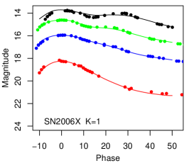
Figure 3: Light curve fitting examples with different component numbers $K$. Each row is for one SNIa with $K=1,2,3$. The red, blue, green and black points are $B+3$, $V+2$, $R+1$, $I$, respectively. Constants are added to the magnitude to separate different bands.

Figure 4: Light curve fitting examples with different component numbers $K$. Each row is for one SNIa with $K=1,2,3$. The red, blue, green and black points are $B+3$, $V+2$, $R+1$, $I$, respectively. Constants are added to the magnitude to separate different bands.

Figure 2 shows the estimated mean functions and the effects of the principal component functions. Each row corresponds to one band $\lambda\in\{B,V,R,I\}$, and each column corresponds to one component $k=1,2,3,4$. In each panel, the solid line is the mean function $\phi_{0\lambda}(q)$. The “$+$” points stand for $\phi_{0\lambda}(q)+2\sigma_{k\lambda}\phi_{k\lambda}(q)$, and the “$-$” points stand for $\phi_{0\lambda}(q)-2\sigma_{k\lambda}\phi_{k\lambda}(q)$ for $k=1,2,3,4$. The $\sigma_{k\lambda}$ is the standard deviation of the score $\beta_{\lambda}^{(k)}$ in the training data. Under the Gaussian assumption, the value $\pm 2\sigma_{k\lambda}$ reflect 95% of the score variability.

Most of the principal component functions have a clear interpretation. We take the $B$-band result (the first row in Figure 2) as an example, and the other bands can be interpreted similarly. The first principal component function $\phi_{1B}(q)$ adjusts the width of the whole light curve, as the “$+$” points are all below the mean function while the “$-$” points are all above the mean function. The second principal component function $\phi_{2B}(q)$ adjusts the decline rate after the peak. Notice the “$+$” points are relatively flat around the peak, and then decline fast after 10 days from the peak. The third principal component function adjusts the brightening rate before the peak. Meanwhile, the fourth principal component function contributes minor and more complex adjustment.

Note that our analysis does not extend beyond 10 days before maximum. Important constraints from very early observations may become available when more SNIa are discovered at very early phases. Moreover, since our light curve model construction is fully data-driven, it can incorporate supernovae that do not agree with the light curve stretch model (Goldhaber et al., 2001).

The effect of higher order principal component functions on the shape of the light curve is usually much less prominent since they explain much smaller proportion of the total variability. We now focus on the first two principal components. The first and second principal component functions describe the width of different parts of the light curve. The scatterplot of the first two scores is in Figure 5. Most of SNIa forms one cluster around the origin in each panel. For a subgroup of SNIa with $B$-band $\Delta M_{15}>1.6$ (purple points), their scores appear off the central cluster and exhibits unique correlation pattern. Notice this group contains SN 1991bg-like fast decliners. In this regard, our light curve model has the potential of sub-grouping SNIa into finer types.

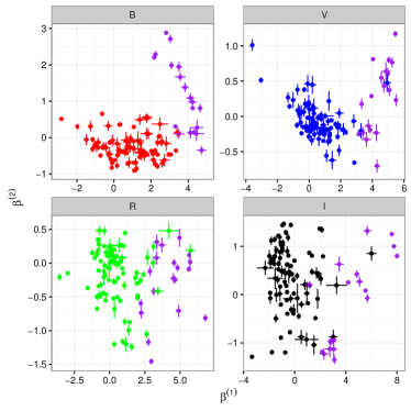
Figure 5: Relation of the first two scores $\beta^{(1)}$ and $\beta^{(2)}$. The $B$, $V$, $R$, $I$ band points are red, blue, green, and black, respectively. The purple points have $B$-band $\Delta M_{15}>1.6$.

For comparison purpose, we also derive the light curve decline rate $\Delta M_{15}$ (Phillips, 1993) based on our estimated light curves. The $\Delta M_{15}$ parameter is calculated for the light curve of each band. It is not a surprise that the scores $\beta^{(1)}$ and $\beta^{(2)}$ are highly correlated with the $\Delta M_{15}$ parameter, as shown in Figure 6. The lack of a tight correlations of light curve decline rates in different colors among themselves and with the PCA scores indicates that no single parameter model such as $\Delta M_{15}$ is able to completely capture the family of SNIa light curve shapes, at least in linear PCA construction, although that single parameter may be found to be strongly correlated with the peak absolute magnitudes of SNeIa (see §7 for more details).

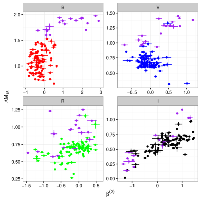
Figure 6: The first two scores $\beta^{(1)}$ (left four panels), $\beta^{(2)}$ (right four panels) against $\Delta M_{15}$. Note in each panel, both the score and $\Delta M_{15}$ are with respect to the corresponding band. The $B$, $V$, $R$, $I$ band points are red, blue, green, and black, respectively. The purple points have $B$-band $\Delta M_{15}>1.6$.

Phillips et al. (1999), Nugent et al. (2002) and Wang (2005) have noticed that severe reddening can shift the mean wavelength of the filter bands and affect the shape of the light curves. This effect is likely to be very small and would not significantly affect the light curve shape parameters we have deduced. The effect of reddening is more easily deduced by comparing the observed color with the light curve scores. Figure 7 shows the first score are nonlinearly correlated with the observed color at $B$ band maximal. For $V$, $R$ and $I$ band light curves, intrinsically redder supernovae tend to have larger values of $\beta^{(1)}$. In Figure 7, the correlations between color and $\beta^{(1)}_{V}$, $\beta^{(1)}_{R}$, $\beta^{(1)}_{I}$. are clean, and show promise for robust separation of intrinsic color and interstellar reddening (see §5). Note that all of the quantities used in Figure 7 are measured from the shape of the light curves and do not require information of supernova distance and reddening.

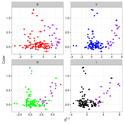
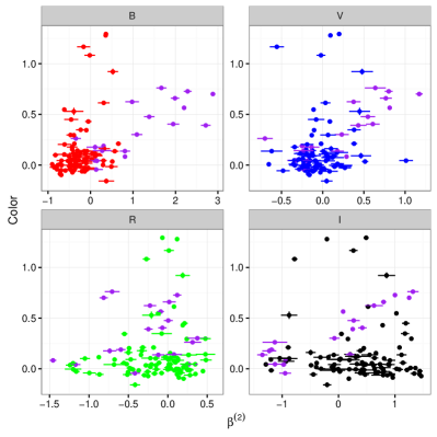
Figure 7: The first two scores $\beta^{(1)}$ (left four panels), $\beta^{(2)}$ (right four panels) against color at $B$-band maximum, $(B-V)_{\mathrm{max}}$. The $B$, $V$, $R$, $I$ band points are red, blue, green, and black, respectively. The purple points have $B$-band $\Delta M_{15}>1.6$.

5 Estimation of Color Excess

Figure 7 reveals a relation between the observed color $(B-V)_{\max}$ at $B$ maximum and the first score $\beta^{(1)}$, especially for $V$, $R$, $I$ band light curves. This relation can be exploited to obtain an estimate of the color excess of the supernova. For example, here we use the relationship between the $R$ band score $\beta^{(1)}_{R}$ and the observed color at $B$ maximum. In Figure 8, we show a lower envelope (the black solid line), and treat it as an extinction free curve for SNIa. This lower envelope is estimated by lower 10% quantile regression with B-spline basis. The quantile regression is iterated by removing points with large positive residuals. This lower envelop $e_{R}(\beta^{(1)}_{R})$ as a function of $\beta^{(1)}_{R}$ serves to estimate the intrinsic color $(B-V)_{0}$ of the supernova. The color excess is obtained by

$$E(B-V)=(B-V)_{\mathrm{max}}-e_{R}(\beta_{R}^{(1)})\ .$$ (7)

In other words, the color excess is the vertical distance from the observation points to the lower envelope, as illustrated in Figure 8.

The same method can be used to estimate extinction using similar relations appeared in other filter bands. The values and precisions from these different measurements however, can be quite different. The lower bound to the $B$ band $\beta^{(1)}_{B}$ shows very little correlation with color, and one would get an estimate of $E(B-V)$ by approximately assuming the intrinsic $B-V$ is nearly zero. In the $V$, $R$, $I$ bands, $\beta^{(1)}$ appears to produce very good intrinsic color estimators.

The popular method to estimate the color excess is from the work of Phillips et al. (1999). They used the empirical linear relation of the intrinsic color $(B-V)_{0}$,

$$(B-V)_{0}=0.725-0.0118\,(q_{V}-60)\ ,$$

for phase $q_{V}$ with respect to the $V$ band maximum. This linear relation holds for $30\leq q_{V}\leq 90$. The color excess can be estimated via the observed color minus the $(B-V)_{0}$ as above. The observed color should be corrected by K-correction and Galactic reddening. Figure 9 compares the color excess computed via this classical method at a reference phase $q_{V}=35$ , and the color excess estimated from the $R$ band score $\beta^{(1)}_{R}$. The figure shows that the color excess given by the method of Lira (1996) and Phillips et al. (1999) has negative values for a considerable portion of the supernovae. Riess et al. (1998) and Jha et al. (2007) (Equation 3) applied a Bayesian approach to produce non-negative color excess estimation. The figure also shows that the uncertainty deduced from $\beta_{R}^{(1)}$ is much smaller than that based on Phillips et al. (1999). This is not surprising, because the method of Phillips et al. (1999) uses only light curve observations beyond 30 days after $V$ band maximum, which are usually very sparse, while our estimation of $\beta_{R}^{(1)}$ uses observations from the whole light curve. The S/N ratios are vastly improved in our approach. Part of the reason that the Lira relation predicts more negative extinction is due to the low S/N ratio of color estimation. Other methods of deducing extinction estimates such as shown in Wang et al. (2005) may also be interesting for further investigation.

Figure 8: The lower envelope (black solid line) for the observed color and $R$ band score $\beta^{(1)}_{R}$. The color excess is estimated by the vertical distance of the observation points to the envelope line.

Figure 9: The y-axis is the color excess computed from Phillips et al. (1999), and the horizontal axis is the color excess computed from the $R$ band score $\beta^{(1)}_{R}$.

6 Spectral Information

This section examines the relationship between the scores in model (3) and spectral features, and discuss the possibility of using the scores for identifying spectral classes. There exists some analysis regarding light curve width and spectral features such as Si II $\lambda$4000 in the literature. With the aid of model (3), we are able to present more details on how light curve shape (not just its width) changes with spectral features. We will also demonstrate the light curve scores can be linked to spectroscopically different SNIa. This linkage is important. With refined spectral subclasses, the K-correction can be applied with higher precision. Identifying sub-classes of SNIa is of ultimate importance in assessing systematic evolutionary effect when applying SNIa as standard candles.

6.1 The Scores and Spectral Features

Figure 10: The heatmap showing correlation between the scores by our FPCA model and the spectral features. The horizontal axis corresponds to the first four scores across all of the $B$, $V$, $R$, $I$ bands. The vertical axis corresponds to various spectral features.

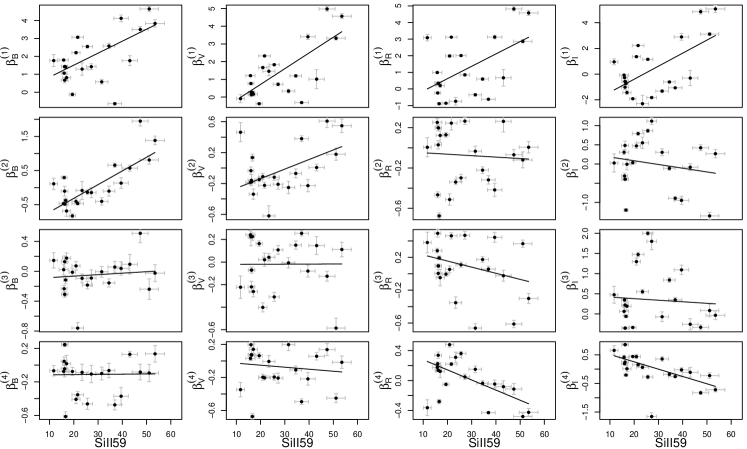
Figure 11: The scores $\beta^{(k)}_{\lambda}$ against the pseudo-equivalent width (pEW) of Si II $\lambda$5972. The points are fitted by a robust linear regression (the solid line).

Figure 12: The “average” light curve shape at four different levels of the pseudo-equivalent width (pEW) of Si II $\lambda$5972.

The dataset of SNIa with comprehensive spectral data is sparse, and the measurement of the strength of spectral features usually suffers from severe systematic errors due to difficulties in defining the level of continuum and observational noise; the latter is usually not even available for most published SNIa spectra. Wagers et al. (2010) developed a mathematical framework based on wavelet decomposition of the spectra to reconstruct the signal from published data. It was shown in Wagers et al. (2010) that large noise can easily bias estimate of spectral line strength, and Monte-Carlo simulation can be used to simulate the effect and correct the bias. However, there is no overlap of the SNIa sample in Wagers et al. (2010) and the current sample. A more recent derivation of spectral line strength is given in Zhao et al. (2016), but its data sample size is small.

High quality spectral feature measurements are scarce. They provide detailed information on the spectral features, which can significantly affect the measured colors and lead to abnormal extinction behavior. The spectral features provide further constraints on the intrinsic properties of supernovae and associated extinction. Measurement of spectral features may prove to be critical for the WFIRST program (Spergel et al., 2013) which aims at unprecedented precision.

We show in this paper the correlations of the most significant spectral features with the light curve features produced from our method. Here we will only use the spectral features extracted by Silverman et al. (2012b), including pseudo-equivalent width (pEW), spectral feature depths, and fluxes at the center and end points of nine spectral feature complexes. The nine spectral feature complexes are Ca II H&K, Si II $\lambda$4000, Mg II, Fe II, Si II ‘W’, Si II $\lambda$5972, Si II $\lambda$6355, O I triplet, Ca II near-IR triplet. We will correlate the first four original scores $\beta^{(1)},\beta^{(2)},\beta^{(3)},\beta^{(4)}$ with the pseudo-equivalent width (pEW) of these spectral feature.

The pEW of the spectral features within 5 days of the $B$ maximum are obtained, and their Spearman correlation coefficients with the scores are computed. The correlation is visualized as heatmap in Figure 10. These nine spectral features corresponds to the first nine rows in the figure. Its columns from left to right correspond to the scores $\beta^{(1)}_{B},\beta^{(1)}_{V},\beta^{(1)}_{R},\beta^{(1)}_{I},\beta^{(2)}_{B},\cdots,\beta^{(4)}_{I}$ respectively. Saturated red (blue resp.) implies a strong positive (negative resp.) correlation; and white color implies a very weak correlation.

The spectral feature Si II $\lambda$4000 and Si II $\lambda$5972 are important spectral luminosity indicator (Nugent et al., 1995). With the light curve width parameter from the SALT II model, Silverman et al. (2012a) noticed that these two features are correlated with light curve width. This is also confirmed in our dataset. Both of them have strong (positive) correlation with the first two scores across four optical bands. The exception is that $\beta^{(2)}_{R}$ has weak (negative) anti-correlation with these two spectral features. We have also shown in Figure 6 the correlation of $\Delta M_{15}$ with the first two scores. The correlations among the spectral feature, our model scores, and the $\Delta M_{15}$ imply that with sufficient amount of well calibrated data it would be possible to construct light curve templates for different spectral sub-classes of SNIa.

This effect on light curve shape is illustrated in Figure 12, which shows the “average” light curve shapes for each band at different levels of pEW(Si II $\lambda$5972). The scores as a function of pEW(Si II $\lambda$5972) is fitted by a robust linear regression, shown as the solid line in Figure 11. Then we compute the value of $\beta^{(k)}_{\lambda}$ at pEW$\approx 13.44,27.95,42.45,56.96$ for $k=1,2,3,4$ and $\lambda\in\{B,V,R,I\}$. After that, the average light curve shapes are computed as $\phi_{0\lambda}(q)+\sum_{k=1}^{4}\beta^{(k)}_{\lambda}\phi_{k\lambda}(q)$ for each filter $\lambda$. Of special interest is the lower right panel of Figure 12. As expected from the previous analysis, when the strength of Si II $\lambda$5972 increases, the $I$ band light curve becomes wider around the peak, but narrower after +15 days in phase. On the other hand, the $B$ band and $V$ band light curves become uniformly narrower across the entire phase range.

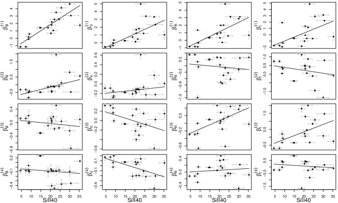
Figure 28: The scores $\beta^{(k)}_{\lambda}$ against the pseudo-equivalent width (pEW) of Si II $\lambda$4000.

A parallel result could be drawn for the spectral feature Si II $\lambda$4000. Its graphical result is in the appendix. The correlation between the scores and Si II $\lambda$4000 is in Figure 28. This correlation pattern resembles that in Figure 11. The “average” light curve shapes corresponding to different levels of Si II $\lambda$4000 are plotted in Figure 29.

Next, we consider five spectral ratios as defined by Silverman et al. (2012a). The first is the Si II ratio, which is the pEW of Si II $\lambda$5972 divided by the pEW of Si II $\lambda$6355,

$$\mathcal{R}(\mathrm{Si\ II})=\frac{\mathrm{pEW(Si~{}{\small II}~{}\lambda 5972)}}{\mathrm{pEW(Si~{}{\small II}~{}\lambda 6355)}}\,.$$

The second is the ratio $\mathcal{R}(\mathrm{Ca\ II})$ of the flux at the red and blue end of Ca II H&K,

$$\mathcal{R}(\mathrm{Ca\ II})=\frac{\mathrm{F_{r}(Ca~{}{\small II}~{}H\&K)}}{\mathrm{F_{b}(Ca~{}{\small II}~{}H\&K)}}\,.$$

These two spectral feature ratios are among the first spectral luminosity indicators (Nugent et al., 1995). Three additional spectral ratios are defined as

$$\begin{split}\mathcal{R}(\mathrm{SiS})&=\frac{\mathrm{F_{r}(S~{}{\small II}~{}W)}}{\mathrm{F_{r}(Si~{}{\small II}~{}\lambda 6355)}}\,,\\ \mathcal{R}(\mathrm{SSi})&=\frac{\mathrm{pEW(S~{}{\small II}~{}W)}}{\mathrm{pEW(Si~{}{\small II}~{}\lambda 5972)}}\,,\\ \mathcal{R}(\mathrm{SiFe})&=\frac{\mathrm{pEW(Si~{}II~{}\lambda 5972)}}{\mathrm{pEW(Fe~{}II)}}\,.\\ \end{split}$$

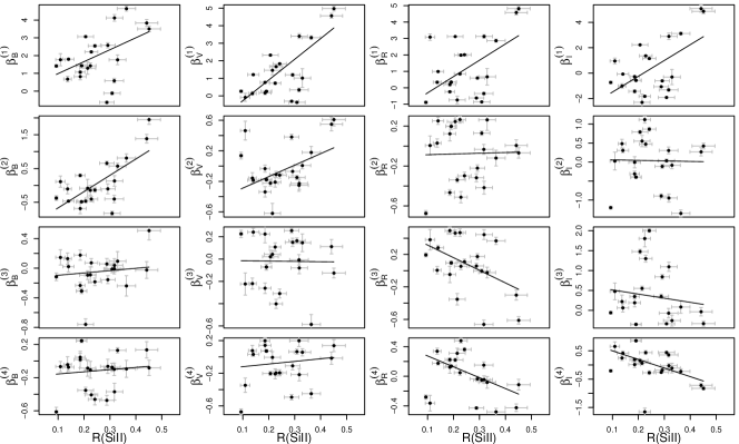
Figure 30: The scores $\beta^{(k)}_{\lambda}$ against the pseudo-equivalent width (pEW) of $\mathcal{R}(\mathrm{Si\ II})$.

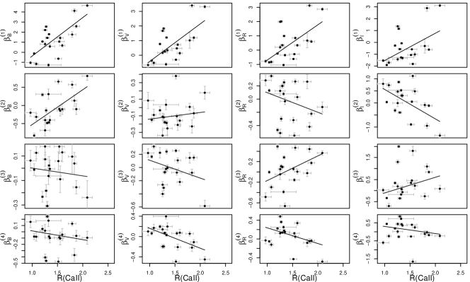
Figure 32: The scores $\beta^{(k)}_{\lambda}$ against the pseudo-equivalent width (pEW) of $\mathcal{R}(\mathrm{Ca\ II})$.

These five ratios correspond to the last five rows in Figure 10. They also have strong correlation (or anti-correlation) with the scores across all four bands. Notice the correlation of $\beta_{R}^{(2)}$ and $\beta^{(2)}_{I}$ tend to have opposite sign with the correlations involving $\beta^{(1)}_{B},\beta^{(1)}_{V},\beta^{(1)}_{R},\beta^{(1)}_{I},\beta^{(2)}_{B},\beta^{(2)}_{V}$. The Figure 30, Figure 31, Figure 32 and Figure 33 in the appendix provide more illustrations about the relation of the scores with $\mathcal{R}(\mathrm{Si\ II})$ and $\mathcal{R}(\mathrm{Ca\ II})$.

6.2 The Scores and Spectral Classes

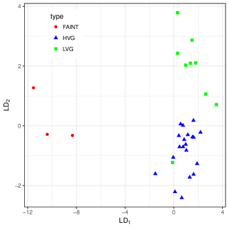
Figure 13: Spectral classes separation of Benetti et al. (2005) using linear discriminant analysis of light curve principal component scores. The SNIa of FAINT, high temporal velocity gradient (HVG) and low temporal velocity gradient group (LVG) are plotted as red circle, blue triangle, and green square, respectively.

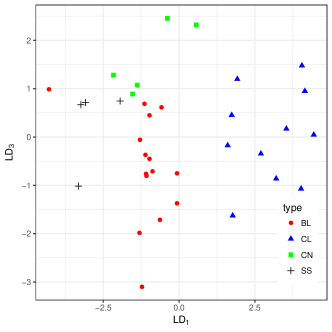
Figure 14: Spectral classes separation of Branch et al. (2009). The spectral class core normal (CN), broad line (BL), cool (CL), and shallow silicon (SS) are shown as green square, red circle, blue triangle and black cross, respectively.

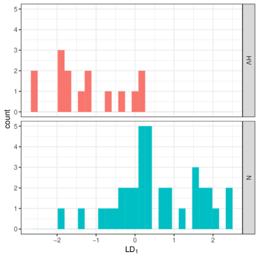
Figure 15: Spectral classes separation of Wang et al. (2009). The histogram of the high velocity (HV) and normal (N) group are plotted in the upper and lower panel, respectively.

Section 6.1 explained that the scores from our FPCA model provide abundant information about spectral features. This section tries to determine supernova spectral classes based on the scores. The task is a standard classification problem well-studied in statistics. We can possibly treat spectral classes as the response, and our scores as predictors. We try to separate spectral classes with the aid of linear discriminant analysis (LDA, Murphy, 2012). In the following, we take the spectral classes from Benetti et al. (2005), Branch et al. (2009), and Wang et al. (2009). We will use all the SNIa in our sample with spectral classes assigned by these papers.

Firstly, we consider the three spectral classes in Benetti et al. (2005). The three classes are FAINT, high temporal velocity gradient (HVG) and low temporal velocity gradient group (LVG). The average velocity gradients in the three groups are 87, 97, and 37, respectively. The resulting $\mathrm{LD}_{1}$ and $\mathrm{LD}_{2}$ are shown in Figure 13.

Branch et al. (2009) provided spectral classification on the basis of the absorption features near 5750Å and 6100Å. The absorption features are measured by pseudo equivalent width. Their four groups are core normal (CN), broad line (BL), cool (CL), and shallow silicon (SS). The CN is a homogeneous class, and its absolute magnitude has a small correlation with light curve width $\Delta M_{15}$. The BL class tends to have strong absorption near 6100Å. For the CL class, the absorption features near 5750Å and 6100Å are both strong; and the SS class is another extreme with both features being weak. On average, the CL class tends to have higher $\Delta M_{15}$ values and fainter absolute magnitude; on the contrary, the SS class tend to have lower $\Delta M_{15}$ values and brighter absolute magnitude. Figure 14 presents the four classes separation based on three linear discriminants.

In Wang et al. (2009), the supernova samples are classified into two groups Normal (N) and high velocity (HV) according to the observed velocity of Si II $\lambda$6355. They found that the HV group has narrower distribution in peak luminosity and decline rate, and this group also prefers a lower extinction ratio. The distance prediction model was applied to these two groups separately to reduce the dispersion in their work.

When only light curve observation is available, Figure 13 and Figure 14 show that we are able to classify the observation into their corresponding spectral classes. However, even if a quantitative scheme proves to be difficult, as illustrated by the class separation result in Figure 15, we could still try to extract a subgroup of SNIa which could be more homogeneous than the entire sample. This is useful in controlling systematic errors in distance determination.

7 Distance Prediction

Our FPCA light curve model can produce the entire shape of a light curve, which in turn can be used for intrinsic luminosity adjustment in distance prediction. In this section, we consider an adjustment using a functional linear form and compare it with the standard adjustment using $\Delta M_{15}$. We consider both the peak magnitude and the CMAGIC magnitude as distance indicators in separate subsections. Note that in this comparative study, the purpose is to show the potential advantage of using the entire light curve shape, and we still use our FPCA model to determine the value of $\Delta M_{15}$.

7.1 Distance Models

Distance models fit a linear model for the distance modulus. The distance modulus $\mu$ is a function of redshift. In particular,

$$\mu(z)=25+5\log_{10}(D_{L}(z)\mathrm{Mpc^{-1}})\,,$$

where $D_{L}(z)$ is the luminosity distance under a fixed cosmology with $\Omega_{m}=0.3$, $\Omega_{\Lambda}=0.7$ and Hubble constant $h=0.7$. With type Ia supernova, the standard model for predicting distance is

$$(M1)\quad\mu=m_{B}-M -\alpha(C-\langle C\rangle)$$

$$-\delta(\Delta M_{15}-\langle\Delta M_{15}\rangle).$$ (8)

In the above, $m_{B}$ is the apparent $B$ band peak magnitude, $M$ is the absolute $B$ band peak magnitude. All these are magnitudes in the rest-frame filter. $C$ is the observed color at $B$ maximum, $(B-V)_{\mathrm{max}}$. $\Delta M_{15}$ is the magnitude change 15 days after $B$ maximum for the $B$ band light curve.

Although simple by concept, $\Delta M_{15}$ is not a quantity that can be directly measured accurately. Its calculated value is highly influenced by light curve fitting errors. In practice, because of the rapid luminosity decay at 15 days past optical maximum, a small error in determining the peak epoch can lead to large inaccuracy of $\Delta M_{15}$.

With our proposed FPCA light curve model, we consider an alternative adjustment of intrinsic luminosity using the entire shape of the light curve. The shape parameter $\Delta M_{15}$ is replaced by a functional linear term

$$Q=\int\delta(q)\{g_{B}(q)-m_{B}-\phi_{0B}(q)\}\mathrm{d}q\,,$$ (9)

where $\delta(q)$ is a fixed function to be determined by the data. Note that in Equation (9), the peak magnitude $m_{B}$ and the mean function $\phi_{0B}(q)$ are subtracted, so that only the light curve shape may influence the value of $Q$. With this functional linear form, the distance model becomes

$$(M2)\quad\mu=m_{B} -M-\alpha(C-\langle C\rangle)$$

$$-(Q-\langle Q\rangle).$$ (10)

Since the light curve shape enters the model as a functional linear term, we refer to (9) as a functional linear distance model. This model has some similarity to the functional linear regression model studied in statistics (Müller & Stadtmüller, 2005).

For each supernova, the associated distance prediction uncertainty includes the parts due to peculiar velocity, measurement error in the apparent magnitude, and intrinsic Type Ia supernova property variation. In the following we assume a peculiar velocity of $v_{\mathrm{pec}}=300\mathrm{\ km\ s}^{-1}$. It introduces magnitude uncertainty of $\sigma_{\mathrm{pec}}=(5/\ln 10)(v_{\mathrm{pec}}/cz)=0.002173/z$, where $c$ is the speed of light. The uncertainty of the apparent peak magnitude $\sigma_{m}$ is computed from the bootstrap method. The associated distance prediction uncertainty is computed as $\sigma_{s}^{2}=\sigma^{2}_{\mathrm{pec}}+\sigma_{m}^{2}$.

The standard distance model (8) is trained by minimizing the $\chi^{2}$,

$$\begin{split}\sum_{s=1}^{S}\frac{1}{\sigma_{s}^{2}}[\mu-m_{B}&+M+\alpha(C-\langle C\rangle)\\ &+\delta(\Delta M_{15}-\langle\Delta M_{15}\rangle)]^{2}\,,\end{split}$$ (11)

where $\Delta M_{15}$ is determined using our FPCA model. The minimization is taken with respect to $M,\alpha,\delta$. A similar $\chi^{2}$ minimization applies to model (10). The functional linear distance model (10) is trained by minimizing

$$\begin{split}\sum_{s=1}^{S}&\frac{1}{\sigma_{s}^{2}}[\mu-m_{B}+M+\alpha(C-\langle C\rangle)\\ &+(Q-\langle Q\rangle)+\eta\int[\delta^{\prime\prime}(q)]^{2}\mathrm{d}q.\end{split}$$ (12)

The minimization is taken with respect to $M$, $\alpha$ and $\delta(q)$ in $Q$. The last term is the integration of the squared second order derivative of $\delta(q)$. This is a roughness penalty to encourage the smoothness of the solution of $\delta(q)$. The $\eta$ parameter controls the amount of penalty imposed and is chosen by the cross-validation. In the minimization of Equation (12), the solution of $\delta(q)$ is searched among the span of the principal component functions $\phi_{k}(q)$, i.e., $\delta(q)=\sum^{K}_{k=1}\delta^{(k)}\phi_{k}(q)$. Using the principal component functions, we only need to solve for the scalar $\delta^{(k)}$’s to get an estimate of the function $\delta(q)$.

7.2 Comparing the Distance Prediction Models

The leave-one-out cross-validation is used to compare the distance prediction models: M1 (Equation 8), M2 (Equation 10), the SALT II $\Delta M_{15}$ model S1, and the SALT II shape parameter model S2. Cross-validation (Section 6.5.3 of Murphy, 2012) is a commonly used method in statistics to evaluate the out-of-sample performance of a prediction model. It works as follows. Each time one sample (i.e. one SNIa) is removed from the dataset, and the remaining dataset is used to train the distance prediction model. The resulted model is then applied to the removed sample to get a predicted distance modulus $\hat{\mu}$. The cross-validated error of this prediction is denoted as $\Delta\mu=\mu-\hat{\mu}$. We repeat this procedure for all SNIa samples in the dataset and summarize the cross-validated errors by the weighted mean squared errors (WMS),

$$\mathrm{WMS}_{cv}=(\sum_{s}\Delta\mu_{s}^{2}/\sigma_{s}^{2})/(\sum_{s}1/\sigma_{s}^{2})\,,$$

whose square-root is $\text{WRMS}_{cv}=\text{WMS}_{cv}^{1/2}$.

Before applying the model to our dataset, we make a further selection of the dataset. We select the SNIa observations with CMB redshift $z>0.01$ and the observed color $(B-V)_{\mathrm{max}}<CC$ for several values of $CC$. The cut $0.01$ on redshift restricts the uncertainty due to peculiar velocity. In addiction, the cut $CC$ on the observed color helps us to select a homogenous group of supernovae.

The result is shown in Table 1. In the table, the $\mathrm{WRMS}_{cv}$ is computed using cross-validated errors. The $\chi^{2}$ is computed using in-sample errors. For example, the result for $CC=0.05$ is given on the first row. With the cut of $z>0.01$ and $(B-V)_{\mathrm{max}}<(0.05)$, there are 37 SNIa in the remaining sample. The $\Delta M_{15}$ model (8) results in a $\mathrm{WRMS}_{cv}$ of 0.089, and the functional linear distance model (10) has a close $\mathrm{WRMS}_{cv}$ of 0.091. The difference of the four models is not significant. With only shape and color information, all models appear to have approached the statistical limits of the data in constructing a Hubble diagram with minimal dispersion. The dispersion is dominated by the peculiar velocity. However, the functional linear distance model (10) consistently produces smaller $\mathrm{WRMS}_{cv}$ across different sample groups. As the value of $CC$ increases, the $\mathrm{WRMS}_{cv}$ for model (10) is stable at the level of $\sim 0.120$. The $\mathrm{WRMS}_{cv}$ for the other models increases to more than $0.14$.

Table 1: Comparison of the distance models

		S1		S2		M1			M2
$CC$	$N$	$\mathrm{WRMS}_{cv}$	$\chi^{2}$	$\mathrm{WRMS}_{cv}$	$\chi^{2}$	$\mathrm{WRMS}_{cv}$	$\chi^{2}$	DOF	$\mathrm{WRMS}_{cv}$	$\chi^{2}$	DOF
$0.05$	37	0.101	127.15	0.108	141.45	0.091	114.34	34.00	0.089	93.37	31.97
$0.1$	48	0.120	255.83	0.127	277.66	0.133	300.04	45.00	0.117	198.32	42.81
$0.2$	62	0.153	487.01	0.162	528.86	0.137	415.53	59.00	0.119	276.56	56.65
$0.3$	65	0.152	509.85	0.162	559.14	0.137	433.16	62.00	0.118	288.45	59.61
$0.4$	67	0.151	514.45	0.161	563.45	0.138	447.91	64.00	0.119	300.58	61.59

At last, we present more detailed results for model (10) at the color cut $CC=0.4$, where the sample size is the largest in our consideration. The upper panel of Figure 16 shows the predicted distance modulus versus redshift velocity. The lower panel of Figure 16 plots the cross-validated residuals and associated error bars. The dashed curves represent the uncertainty due to the assumed peculiar velocity. Note the scatter of the residuals is dominated by peculiar velocity at redshifts around 300 $\mathrm{km}\cdot\mathrm{s}^{-1}$. In addition, the estimated functional coefficient $\delta(q)$ is presented in Figure 17. This functional coefficient $\delta(q)$ is positive over the phase range $(-10,20)$. This suggests that the functional linear form still tries to measure the width of the light curve in its own way, and the measurement is adjusted by the phase range $(20,50)$. Figure 18 compares the quantity $\Delta M_{15}$ with the calculated value of the the functional linear form $\int\delta(q)(g_{B}(q)-m_{B}-\phi_{0B}(q))\mathrm{d}q$.

Figure 16: Predicted distance and residuals of the functional linear distance model. The dashed lines represent the uncertainty due to the peculiar velocity.

Figure 17: The estimated $\delta(q)$ of the functional linear form (9). The solid line is the estimated $\delta(q)$, the dashed lines represent one standard deviation uncertainty.

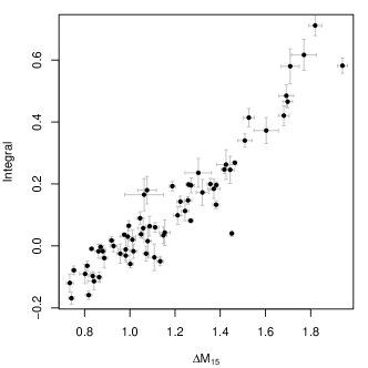
Figure 18: Comparing the $\Delta M_{15}$ on the horizontal axis with the value of the functional linear form $\int\delta(q)(g_{B}(q)-m_{B}-\phi_{0B}(q))\mathrm{d}q$ on the vertical axis.

7.3 The CMAGIC for Distance Prediction

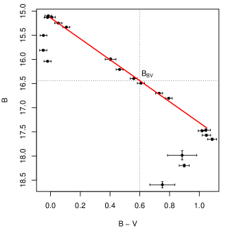
Figure 19: An example of the linear color magnitude evolution after B maximum. The red line is the fitted linear relation. The $B$ band magnitude at $B-V=0.6$ is extracted to get the CMAGIC magnitude $B_{BV}$.

We now evaluate the effectiveness of using the entire light curve shape to adjust intrinsic luminosity for distance predication when the CMAGIC magnitude is used as the distance indicator. The CMAGIC magnitude, proposed by Wang et al. (2003), exploits the linear relation of the color evolution for about 30 days after the $B$ maximum. During this phase the $B$ and $B-V$ magnitude follow a linear trend, as illustrated by the red line in Figure 19.

$$B=B_{BV}+\gamma(B-V-0.6)$$ (13)

where $\gamma$ is the slope of the linear relation. The exact starting and ending epochs of this linear evolution vary among supernovae with their intrinsic brightness. Some supernovae with a small $\Delta M_{15}$ show a “bump” feature in the color magnitude evolution immediately after $B$ maximum. For our supernova samples, the observation points in the $B$ band phase range $[+3,+25]$ are used to fit the linear relation. Wang et al. (2003) noticed that the slope $\gamma$ has a small scattering $0.18$ around the mean of $2.07$.

The CMAGIC magnitude, denoted by $B_{BV}$, is defined as the $B$ band magnitude when $B-V=0.6$. Wang et al. (2003) replaced the peak magnitude $m_{B}$ in (8) by $B_{BV}$ and considered the following model

$$(M3)\quad\mu= B_{BV}-M-\delta(\Delta M_{15}-\langle\Delta M_{15}\rangle)-(b_{2}-\gamma)\times$$

$$[\frac{m_{B}-B_{BV}}{\gamma}+0.6+1.2(\frac{1}{\gamma}-\langle\frac{1}{\gamma}\rangle)]\,,$$ (14)

where $M$, $\delta$ and $b_{2}$ are parameters to be estimated. In this paper, we will use $\Delta M_{15}$ determined by our FPCA model. Besides, as an alternative model, the $\Delta M_{15}$ is replaced by the functional linear form $Q$ defined in Equation (9),

$$(M4)\quad\mu= B_{BV}-M-(Q-\langle Q\rangle)-(b_{2}-\gamma)\times$$

$$\quad[\frac{m_{B}-B_{BV}}{\gamma}+0.6+1.2(\frac{1}{\gamma}-\langle\frac{1}{\gamma}\rangle)]\,.$$ (15)

In order to fit the linear color evolution, with the dataset described in Section 2, at least five observation points is required in the $B$ band phase range $[+3,+25]$. We select those samples with $z>0.01$ and make various levels of cut on the observed color $(B-V)_{\mathrm{max}}$ at $B$ maximum. The color cut is necessary, due to the fact that the linear color evolution and CMAGIC can be best constrained among low $(B-V)_{\mathrm{max}}$ samples. A five sigma cut is also applied to $\gamma$. For the $66$ samples with color cut of 0.3, their slopes $\gamma$ have a mean of 2.15 and standard deviation 0.20.

Over the selected SNIa samples, four models S3, S4, M3 (Equation 14), and M4 in (Equation 15) are tested using the leave-one-out cross-validation procedure as described in Section 7.2. Table 2 presents their $\mathrm{WRMS}_{cv}$, $\chi^{2}$ and degree of freedom (DOF) at different levels of cutoff at the observed color at $B$ maximum. At the cut $0.05$ of the color at $B$ maximum, the model S3, S4 M3 and M4 has a $\mathrm{WRMS}_{cv}$ of $0.145$, $0.149$, $0.119$ and $0.122$, respectively. At the cut $0.4$ of the color at $B$ maximum, the models have $\mathrm{WRMS}_{cv}$ of $0.155$, $0.160$, $0.137$ and $0.135$, respectively. The histogram of the residuals for M4 is ploted in Figure 20. While there are a few samples with large residuals, most samples have residuals with absolute value less than $0.2$. SN 2007ca show significantly larger residual for unknown reasons. It is however the most highly extinguished supernova included in our sample. Notice the sample size $N$ in Table 2 is smaller than in Table 1, because we require at least $5$ observational points in the $B$ band phase range $[+3,+25]$ to constrain the color evolution.

Figure 20: The histogram of cross-validation residuals for M4 at color cut $CC=0.4$.

Table 2: Comparison of the distance models

		S3		S4		M3			M4
$CC$	$N$	$\mathrm{WRMS}_{cv}$	$\chi^{2}$	$\mathrm{WRMS}_{cv}$	$\chi^{2}$	$\mathrm{WRMS}_{cv}$	$\chi^{2}$	DOF	$\mathrm{WRMS}_{cv}$	$\chi^{2}$	DOF
$0.05$	32	0.145	184.13	0.149	195.27	0.119	151.12	29.00	0.122	111.34	26.32
$0.1$	40	0.156	270.95	0.160	281.62	0.137	233.32	37.00	0.130	165.53	34.45
$0.2$	52	0.149	351.53	0.154	371.20	0.130	292.66	49.00	0.130	243.81	46.41
$0.3$	55	0.149	371.92	0.155	397.16	0.129	306.25	52.00	0.128	255.46	49.28
$0.4$	56	0.155	413.60	0.160	435.51	0.137	347.93	53.00	0.135	289.69	50.28

8 Results from the fv-FPCA model

Figure 21: Results from the fv-FPCA model. Plots of $\phi_{0}(q)\pm 2\phi_{j}(q)$ for the first four principal components functions. This shows how these functions change the shape of light curve. The solid line in each panel is the mean function. The “$+$” points represent $\phi_{0}(q)+2\phi_{j}(q)$, and the “$-$” points represent $\phi_{0}(q)-2\phi_{j}(q)$. The vertical scale is given in magnitudes.

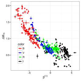
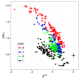
Figure 22: Results from the fv-FPCA model. Relation of the first two scores $\beta^{(1)},\beta^{(2)}$, and $\Delta M_{15}$ for each color band. The left panel is the plot of $\beta^{(1)}$ and $\beta^{(2)}$; the middle panel is the plot of $\beta^{(1)}$ and $\Delta M_{15}$; and the right panel is the plot of $\beta^{(2)}$ and $\Delta M_{15}$. The $B$, $V$, $R$, $I$ band points are red, blue, green, and black, respectively.

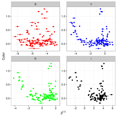
Figure 23: Results from the fv-FPCA model. Plot of the first score $\beta^{(1)}$ against color at $B$-band maximum, $(B-V)_{\mathrm{max}}$.

Figure 24: Results from the fv-FPCA model. Plot of the second score $\beta^{(2)}$ against color at $B$-band maximum, $(B-V)_{\mathrm{max}}$.

In the previous sections, fs-FPCA models (Equation 3) are trained separately using observations from different well-defined optical filters. This approach has a limitation that one has to correct observations to a rest-frame filter before light curve fitting. However, our FPCA method can be employed in another way to overcome this limitation. Specifically, we can pool data from several bands together to train a filter-vague FPCA (fv-FPCA) model (Equation 4), where a single set of mean function and principal component functions are used to describe the light curves of all bands. When fitting a new light curve, the fv-FPCA model can be directly applied to data in their observed filter, and no correction to rest-frame is necessary initially. We illustrate this approach to the same dataset used in previous sections, where the K-corrections have already been applied to the data. Not surprisingly, most of the results remain the same as presented in previous sections. This demonstrates that both approaches are effective in capturing light curve information. We only present below results that are different from previous sections.

The four panels of Figure 21 show the estimated mean function and the effects of a single principal component function. The solid line represents the mean function $\phi_{0}(q)$. The “$+$” points represent $\phi_{0}(q)+2\phi_{j}(q)$, and the “$-$” points represent $\phi_{0}(s)-2\phi_{j}(s)$ for $j=1,2,3,4$. The first principal component function $\phi_{1}(q)$ (shown in the supper left panel) reflects decline rate about 15 days after the peak. The second principal component function $\phi_{2}(q)$ (shown in the upper right panel) is sensitive to the light curve width around the peak. Meanwhile, it also reflects a contrast of decline rate before and after $\sim$ 20 days in phase. The third principal component function (shown in the lower left panel) adjusts the bump around 20 days after the peak. The fourth principal component function (shown in the lower right panel) exhibits more complex fluctuations. For the proportion of variability, the first principal component function explains 91.69% of the total variability, the first two principal component function explains 96.31%, and the first four together explain 99.24%.

As the scores are measured by the same set of principal functions, their values are comparable and can be plotted in one panel. The first two scores are correlated in a nonlinear pattern, as shown in the left panel of Figure 22. What may be especially interesting is the seemingly monotonic shift of the locus of data with filter bands. The left panel of Figure 22 shows $\beta^{(1)}$ increases as the wavelength increases, whereas the range of $\beta^{(2)}$ remains nearly the same. The locus of data points in each filter shows consistent correlation patterns and can be globally shifted to approximately match each other. These characteristics suggest that in principle we are able to derive photometric redshifts based on the scores. These score correlations can also facilitate robust photometric identification of SNIa.

The relation between $\beta^{(1)}$, $\beta^{(2)}$ and $\Delta M_{15}$ are presented in the middle and right panel of Figure 22. Besides, Figure 23 and Figure 24 show that the first and second scores are nonlinearly correlated with the observed color at $B$ band maximal. From here, the color excess can be deduced in a similar way as in Section 5. In addition, all other analysis conducted previously can be carried out, including the spectral information correlation, spectral classification and distance prediction. The messages remain the same as in the previous sections.

Figure 25: Results from the fv-FPCA model. The nonlinear scores $\tilde{\beta}^{(1)},\tilde{\beta}^{(2)}$ are calculated via fitting curves to the original scores $\beta^{(1)},\beta^{(2)}$.

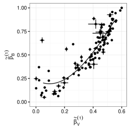
Figure 26: Results from the fv-FPCA model. The relation between the first nonlinear $V$ band score $\tilde{\beta}^{(1)}_{V}$ (on horizontal axes) with $\tilde{\beta}^{(1)}_{B}$, $\tilde{\beta}^{(1)}_{R}$, $\tilde{\beta}^{(1)}_{I}$ (on vertical axes).

Figure 27: Results from the fv-FPCA model. Average light curve shapes parametrized by the nonlinear score $\tilde{\beta}_{V}^{(1)}$.

A final point to notice is the potential of more effective dimension reduction with nonlinear dimension reduction techniques. This is due to the nonlinear relation between the first two dominant scores $\beta^{(1)},\beta^{(2)}$ in Figure 22. For simplicity, consider the two dimensional space of $\beta^{(1)}$ and $\beta^{(2)}$. These first two dimensions alone already account for 96.31% cumulative variance of the dataset. We adapt the concept of principal ridge (Ozertem & Erdogmus, 2011). A curve is fitted for $\beta^{(1)}_{B}$ and $\beta^{(2)}_{B}$ of $B$ band, as the left black solid line in Figure 25. This nonlinear curve is treated as the first nonlinear dimension for $B$ band scores. The second nonlinear dimension is the one locally perpendicular to the curve. Given the original scores $\beta^{(1)},\beta^{(2)}$ from our model, the new nonlinear scores $\tilde{\beta}^{(1)},\tilde{\beta}^{(2)}$ are calculated as follows. Consider the left red point in Figure 25, it is projected onto the $B$ band curve. The projection is identified by the nearest point on the curve. The nonlinear score $\tilde{\beta}^{(1)}$ is the geodesic distance from the leftmost point of the curve to the projection point. The geodesic distance along the curve is indicated by the red dashed curve. The new score $\tilde{\beta}^{(2)}$ is the usual Euclidean distance of the original point to the projection point, as indicated by the red vertical dashed line. In a similar manner, a curve is fitted for $V$, $R$, $I$ band together (the right solid curve in Figure 25), and the linear scores for $V$, $R$, $I$ band are projected onto this curve to obtain the new nonlinear score.

In the original linear system, the first dimension explains 91.69% of the total variability. The first two dimension together explains 96.31% of the total variability. Now in the nonlinear system, the explained proportion of the first nonlinear score should be larger than 91.69%, but smaller than 96.31%. More light curve information is absorbed into the first dimension. The first score alone can provide adequate fit to SNIa light curves.

The more thorough dimension reduction can be made by describing the correlation among $\tilde{\beta}^{(1)}_{B},\tilde{\beta}^{(1)}_{V},\tilde{\beta}^{(1)}_{R},\tilde{\beta}^{(1)}_{I}$. The shape of light curves across these optical bands should be well correlated due to their common spectral evolution. The relation of $\tilde{\beta}^{(1)}_{V}$ with $\tilde{\beta}^{(1)}_{B},\tilde{\beta}^{(1)}_{R},\tilde{\beta}^{(1)}_{I}$ is plotted in Figure 26. For most of the cases, the $V$ band nonlinear score $\tilde{\beta}^{(1)}_{V}$ is a reliable predictor of $\tilde{\beta}^{(1)}_{B},\tilde{\beta}^{(1)}_{R}$ and $\tilde{\beta}^{(1)}_{I}$. Therefore we can use a single parameter, $\tilde{\beta}^{(1)}_{V}$, to describe all the SNIa light curve shapes. For each $\tilde{\beta}^{(1)}_{V}$, the predicted values of $\tilde{\beta}^{(1)}_{B},\tilde{\beta}^{(1)}_{R}$ and $\tilde{\beta}^{(1)}_{I}$ are obtained by the fitted curves in Figure 26. This single parameterization of light curve shape is especially useful for fitting high redshift supernovae with sparse and noisy observations, because only one parameter is required to be constrained by the data. Using this scheme with a single parameter $\tilde{\beta}^{(1)}_{V}$, Figure 27 depicts all four band light curve shapes for $\tilde{\beta}^{(1)}_{V}=0.05,0.2,0.35,0.5$. These light curves are the expected shapes accounting for first order correction of the mean curve with $\tilde{\beta}^{(1)}_{V}$.

9 Discussions and Conclusions

We have presented in this paper an empirical model for SNIa light curves. Using this model, the entire light curve of a SNIa can be represented by a few scores. These scores characterize light curve shape, intrinsic color, and color excess for SNIa. Some light curve scores are even correlated with spectral features measured independently of SNIa light curves. In previous studies, the absorption features of SNIa spectra have been empirically compared with the color and the light curve width parameter. For example, Silverman et al. (2012a) showed the strength of Si II $\lambda$4000 is anti-correlated with SALT II width parameter and uncorrelated with color. This anti-correlation only implies stronger Si II $\lambda$4000 correlated with narrower light curve shape. However it is interesting to explore further how the light curve shape in multi-bands changes with the strength of this line. The score parameters from our model reveal more such information. Regarding this, we have presented a more detailed morphology analysis of light curve with respect to the feature strength.

Beyond these empirical investigations, the proposed model embraces more potential in cosmology model fitting. Although the primary light curve shape parameter such as $\Delta M_{15}$, the stretch parameter, or the parameter in SALT II is effective, it is still worthwhile to explore other constructions using the shape of the entire light curve. Estimation of $\Delta M_{15}$ is sensitive to local observations around the peak and around the +15 days in phase. If we lack enough observations to constraint light curve shapes around these days in phase, the estimated $\Delta M_{15}$ would have large uncertainty. Besides, the $\Delta M_{15}$ parameter only captures the declining part of the light curves, and fails to capture the light curve shape at the rising side. The stretch parameter may not be applicable for SN wavelength bands longer than $I$ band, and may not always fit well for both the rising and falling part of a SNIa light curve. A product of our FPCA model is to replace the $\Delta M_{15}$ term in the existing distance prediction models by a functional linear term, which provides a more flexible and data-driven way to adjust the light curve shape for distance prediction. Comparison with the previous distance models using $\Delta M_{15}$ adjustment and SALT II shape parameter suggests that the functional linear form of the entire light curve has the potential to give smaller residual scattering and robust distance prediction.

Among the effort to reduce distance prediction scatter, one common conjecture is that SNIa is not a homogeneous group. There exist subclasses of their own characteristics. Each subclass has its own dust correction and K-correction. Picking out a more homogeneous subclass help to further reduce the dispersion. Some works endeavor to identify subclasses based on spectral data (Benetti et al., 2005; Branch et al., 2009; Wang et al., 2009). The dispersion reduction is more significant by pairing supernovae with identical spectral features and applying pairwise dust correction (Fakhouri et al., 2015). Our study finds that, when only light curve data is available, the scores extracted from the light curve can still help to determine spectral classes, although with limited precision. Therefore, it is possible to reduce the dispersion by fitting the distance and dust correction model within a subclass of SNIa observations. Another potential application of this result is to improve the precision of K-correction, as the spectral template from the corresponding spectral class can be applied for this subclass of observations.

Precise redshift will be needed if the filter-vague FPCA is used for cosmological distance determination. In future experiments with LSST or WFIRST, the sample size will be significantly larger than today, more parameters can be deduced for controls of systematic effects of SNIa, the PCA approach allows for accurate quantification of information loss in the light curve fitting procedures.

Supplementary Materials

The supplementary materials are available to download at https://github.com/shiyuanhe/supern. The supplementary materials contain the following:

2. The SNIa data table. The data table contains all SNIa samples in this paper with their scores, spectral line strength and spectral class.

3. The FPCA software. The software provides a web-based user interface for light curve fitting, intrinsic color estimation, spectral line strength estimation and spectral classes determination. It also provide the probability that the submitted sample belongs to SNIa.

Appendix A Algorithm

This section presents the details of the model training algorithm used for model training in Section 3.2. The presentation focuses on the fs-FPCA. If data from several bands are pooled together to train the fv-FPCA model (4), the algorithm needs to be modified slightly in an obvious fashion. All light curves are registered with the transformation, $q_{s\lambda j}=(t_{s\lambda j}-b_{s\lambda})/(1+z_{s\lambda})$. This transformation aligns all the light curves such that their peaks are at phase zero. However, the peak epoch $b_{s\lambda}$ is unknown. An initial estimate of the peak magnitude $m_{s\lambda}$ and peak epoch $b_{s\lambda}$ are obtained by a local quadratic regression. With this initial estimate, a two-step procedure is carried out for model training, i.e., learning the mean function $\phi_{0\lambda}(q)$ and learning the principal component functions $\phi_{k\lambda}(q)$’s ($k\geq 1$).

A.1 Learning the Mean Function

If we define $\mathbf{B}_{s\lambda}=\big{(}\mathbf{b}(q_{i1}),\cdots,\mathbf{b}(q_{in_{i}})\big{)}^{T}$, the model (6) in matrix form is

$$\mathbf{y}_{s\lambda}=m_{s\lambda}\mathbf{1}_{n_{s\lambda}}+\mathbf{B}_{s\lambda}\boldsymbol{\theta}_{0}+\mathbf{B}_{s\lambda}\boldsymbol{\Theta}_{\phi}\boldsymbol{\beta}_{s\lambda}+\mathbf{W}_{s\lambda}\boldsymbol{\epsilon}_{s\lambda}\,,$$ (A1)

where $\mathbf{1}_{n_{s\lambda}}$ is a vector of ones with length $n_{s\lambda}$, $\boldsymbol{\epsilon}_{i}$ is a random vector of length $n_{s\lambda}$ following a standard normal distribution, and $\mathbf{W}_{s\lambda}=\text{diag}\{\sigma_{s\lambda 1},\cdots,\sigma_{s\lambda n_{s\lambda}}\}$. This representation includes all the light curve observations of the $s$-th supernova with filter $\lambda$.

The last two terms in (A1) has an expectation of zero. Although their covariance matrix is unknown, the general least square estimate is still consistent with least square estimation. With the estimated peak magnitude $\widehat{m}_{s\lambda}$ and peak epoch $\widehat{b}_{s\lambda}$, we estimate $\boldsymbol{\theta}_{0\lambda}$ by solving

$$\min_{\boldsymbol{\theta}_{0\lambda}}\sum_{s}\frac{1}{n_{s\lambda}}\|(\mathbf{W}_{s\lambda})^{-1}(\mathbf{y}_{s\lambda}-\widehat{m}_{s\lambda}\mathbf{1}_{n_{s\lambda}}-\mathbf{B}_{s\lambda}\boldsymbol{\theta}_{0\lambda})\|^{2}_{2}+\eta\,\text{tr}\big{(}\boldsymbol{\theta}_{0\lambda}^{T}\boldsymbol{\Omega}\boldsymbol{\theta}_{0\lambda}\big{)}$$ (A2)

where $\boldsymbol{\Omega}=\int\mathbf{b}^{\prime\prime}(t)^{T}\mathbf{b}^{\prime\prime}(t)\textrm{d}t$. The last term is the roughness penalty to encourage a smooth solution, and $\eta$ is the tuning parameter. Essentially, the smoothness is achieved by controlling the integral of the squared second order derivative of the solution, i.e., $\int(\phi_{0\lambda}^{\prime\prime}(q))^{2}\mathrm{d}q=\text{tr}\big{(}\boldsymbol{\theta}_{0\lambda}^{T}\boldsymbol{\Omega}\boldsymbol{\theta}_{0\lambda}\big{)}$. Suppose $\widehat{\boldsymbol{\theta}}_{0\lambda}$ is the solution of the optimization problem (A2), then the resulting mean function is $\hat{\phi}_{0\lambda}(q)=\mathbf{b}(q)^{T}\widehat{\boldsymbol{\theta}}_{0\lambda}$.

A.2 Learning the Principal Component Functions

Now align the peak and subtract the mean function from the observed light curves, $\widetilde{\mathbf{y}}_{s\lambda}=\mathbf{y}_{s\lambda}-\widehat{m}_{s\lambda}\mathbf{1}_{n_{s\lambda}}-\mathbf{B}_{s\lambda}\widehat{\boldsymbol{\theta}}_{0\lambda}\,.$ This is the remaining difference to be fitted by the principal component functions $\phi_{k\lambda}(q)$’s.

Let $\mathbf{s}_{s\lambda}=\boldsymbol{\Theta}_{\phi}\boldsymbol{\beta}_{s\lambda}$ and put them in a $P\times S$ matrix $\mathbf{S}_{\lambda}=\left(\mathbf{s}_{1\lambda},\mathbf{s}_{2\lambda},\cdots,\mathbf{s}_{S\lambda}\right)$. We estimate $\mathbf{S}_{\lambda}$ by solving the following optimization problem

$$\min_{\mathbf{S}_{\lambda}}\sum_{s}\frac{1}{n_{s\lambda}}\|(\mathbf{W}_{s\lambda})^{-1}(\widetilde{\mathbf{y}}_{s\lambda}-\mathbf{B}_{s\lambda}\mathbf{s}_{s\lambda})\|^{2}_{2}+\eta_{1}\|\mathbf{S}_{\lambda}\|_{S_{1}}+\eta_{2}\text{tr}\big{(}\mathbf{S}_{\lambda}^{T}\boldsymbol{\Omega}\mathbf{S}_{\lambda}\big{)}\,.$$ (A3)

In the above, $\|\cdot\|_{S_{1}}$ is the nuclear norm penalty, which is the summation of all singular values of a matrix. This penalty encourages a low-rank solution of $\mathbf{S}_{\lambda}$, and thereby encourages a small number $K$ of principal component functions. A roughness penalty $\text{tr}\big{(}\mathbf{S}_{\lambda}^{T}\boldsymbol{\Omega}\mathbf{S}_{\lambda}\big{)}$ is also imposed to ensure each column of the solution $\mathbf{S}_{\lambda}$ is smooth. The tuning parameters, $\eta_{1}$ and $\eta_{2}$, are selected by cross-validation. The rank of $\mathbf{S}_{\lambda}$ is automatically determined by the algorithm. The optimization problem (A3) is solved by the ADMM algorithm (Boyd et al., 2011) combined with the singular value soft-thresholding operator (Cai et al., 2010). The ADMM algorithm breaks the optimization into two easy-to-solve parts: one part involves the quadratic loss and the other involves the nuclear norm. The algorithm then iteratively updates the two parts and the Lagrangian multiplier until convergence.

Now, let $\widehat{\mathbf{S}}_{\lambda}$ be the solution of the optimization problem (A3) for filter $\lambda$, and $\widehat{\mathbf{S}}_{\lambda}=\widehat{\mathbf{U}}_{\lambda}\widehat{\mathbf{D}}_{\lambda}\widehat{\mathbf{V}}^{T}_{\lambda}$ be its SVD decomposition. Suppose $\widehat{\mathbf{u}}_{i\lambda}$ is the $i$-th column of $\widehat{\mathbf{U}}_{\lambda}$. Let $\widehat{\boldsymbol{\Theta}}_{\phi\lambda}=\left(\widehat{\mathbf{u}}_{1\lambda},\widehat{\mathbf{u}}_{2\lambda},\cdots,\widehat{\mathbf{u}}_{K\lambda}\right)$ be estimated by the first $K$ columns of $\widehat{\mathbf{U}}_{\lambda}$, then the estimated principal component functions are $\widehat{\boldsymbol{\phi}}(s)^{T}_{\lambda}=\mathbf{b}(s)^{T}\widehat{\boldsymbol{\Theta}}_{\phi\lambda}$.

Appendix B Fitting Functional Linear Distance Model

Appendix C Supplementary Table

Table 3: Example Supplementary Table

	SNe	Survey	redshift	Type1	Type2	Type3	Bmax	Vmax	B_scores1	V_scores1	R_scores1	I_scores1
1	SN1998de	LOSS	0.0157				17.3320	16.6420	4.2330	5.0700	4.5330	3.4840
2	SN1998dh	LOSS	0.0077				13.8900	13.8220	1.5960	0.9880	0.3940	-0.6010
3	SN1998ef	LOSS	0.0171				14.8560	14.8900	2.3430	0.7600	0.9070	-0.7250
4	SN1999ac	LOSS	0.0098	HVG	CN	N	14.1040	14.0570	1.0680	0.7680	-0.2390	-0.2690
5	SN1999by	LOSS	0.0027				13.5360	13.0720	3.0430	4.7290	4.6650	4.1910
6	SN1999cl	LOSS	0.0081			N	14.8640	13.7560	0.8980	0.5540	0.2940	-0.3570
7	SN1999cp	LOSS	0.0103	LVG	BL	N	13.9470	13.9630	1.2130	0.3600	1.1060	-0.2900
8	SN1999da	LOSS	0.0121	FAINT	CL		16.5980	16.0310	3.8350	4.5650	4.5800	5.0750
9	SN1999dk	LOSS	0.0141				14.8280	14.7550	1.3930	0.7620	0.1030	-0.5770
10	SN1999dq	LOSS	0.0137	HVG	SS		14.4790	14.3650	-0.1200	-0.3700	-0.8570	-1.9100

Appendix D Supplementary Figures

Figure 29: The “average” light curve shape at four different levels of the pseudo-equivalent width (pEW) of Si II $\lambda$4000.

Figure 31: The “average” light curve shape at four different levels of the pseudo-equivalent width (pEW) of $\mathcal{R}(\mathrm{Si\ II})$.

Figure 33: The “average” light curve shape at four different levels of the pseudo-equivalent width (pEW) of $\mathcal{R}(\mathrm{Ca\ II})$.

References

- Benetti et al. (2005) Benetti, S., Cappellaro, E., Mazzali, P. A., et al. 2005, The Astrophysical Journal, 623, 1011
- Blondin et al. (2011) Blondin, S., Mandel, K. S., & Kirshner, R. P. 2011, Astronomy & Astrophysics, 526, A81
- Boyd et al. (2011) Boyd, S., Parikh, N., Chu, E., Peleato, B., & Eckstein, J. 2011, Foundations and Trends® in Machine Learning, 3, 1
- Branch et al. (2009) Branch, D., Dang, L. C., & Baron, E. 2009, Publications of the Astronomical Society of the Pacific, 121, 238
- Burns et al. (2010) Burns, C. R., Stritzinger, M., Phillips, M., et al. 2010, The Astronomical Journal, 141, 19
- Cai et al. (2010) Cai, J.-F., Candès, E. J., & Shen, Z. 2010, SIAM Journal on Optimization, 20, 1956
- Conley et al. (2006) Conley, A., Goldhaber, G., Wang, L., et al. 2006, ApJ, 644, 1
- Conley et al. (2008) Conley, A., Sullivan, M., Hsiao, E., et al. 2008, The Astrophysical Journal, 681, 482
- Contreras et al. (2010) Contreras, C., Hamuy, M., Phillips, M., et al. 2010, The Astronomical Journal, 139, 519
- Efron & Tibshirani (1994) Efron, B., & Tibshirani, R. J. 1994, An introduction to the bootstrap (CRC press)
- Fakhouri et al. (2015) Fakhouri, H., Boone, K., Aldering, G., et al. 2015, The Astrophysical Journal, 815, 58
- Foley et al. (2009) Foley, R. J., Chornock, R., Filippenko, A. V., et al. 2009, The Astronomical Journal, 138, 376
- Ganeshalingam et al. (2010) Ganeshalingam, M., Li, W., Filippenko, A. V., et al. 2010, The Astrophysical Journal Supplement Series, 190, 418
- Goldhaber et al. (2001) Goldhaber, G., Groom, D. E., Kim, A., et al. 2001, ApJ, 558, 359
- Goldhaber et al. (2001) Goldhaber, G., Groom, D., Kim, A., et al. 2001, The Astrophysical Journal, 558, 359
- Guy et al. (2005) Guy, J., Astier, P., Nobili, S., Regnault, N., & Pain, R. 2005, Astronomy & Astrophysics, 443, 781
- Guy et al. (2007) Guy, J., Astier, P., Baumont, S., et al. 2007, Astronomy & Astrophysics, 466, 11
- Hastie et al. (2009) Hastie, T., Tibshirani, R., & Friedman, J. 2009, The elements of statistical learning: data mining, inference and prediction, 2nd edn. (Springer)
- Hicken et al. (2009) Hicken, M., Challis, P., Jha, S., et al. 2009, The Astrophysical Journal, 700, 331
- Hicken et al. (2012) Hicken, M., Challis, P., Kirshner, R. P., et al. 2012, The Astrophysical Journal Supplement Series, 200, 12
- Höflich et al. (1996) Höflich, P., Khokhlov, A., Wheeler, J. C., et al. 1996, ApJ, 472, L81
- Höflich et al. (2010) Höflich, P., Krisciunas, K., Khokhlov, A. M., et al. 2010, ApJ, 710, 444
- Höflich et al. (2017) Höflich, P., Hsiao, E. Y., Ashall, C., et al. 2017, ApJ, 846, 58
- Hsiao et al. (2007) Hsiao, E., Conley, A., Howell, D., et al. 2007, The Astrophysical Journal, 663, 1187
- James et al. (2000) James, G. M., Hastie, T. J., & Sugar, C. A. 2000, Biometrika, 87, 587
- Jha et al. (2007) Jha, S., Riess, A. G., & Kirshner, R. P. 2007, The Astrophysical Journal, 659, 122
- Kasen et al. (2016) Kasen, D., Metzger, B. D., & Bildsten, L. 2016, The Astrophysical Journal, 821, 36
- Lira (1996) Lira, P. 1996, Master’s thesis, MS thesis. Univ. Chile (1996)
- Müller & Stadtmüller (2005) Müller, H.-G., & Stadtmüller, U. 2005, Annals of Statistics, 774
- Murphy (2012) Murphy, K. P. 2012, Machine learning: a probabilistic perspective (MIT press)
- Nugent et al. (2002) Nugent, P., Kim, A., & Perlmutter, S. 2002, Publications of the Astronomical Society of the Pacific, 114, 803
- Nugent et al. (1995) Nugent, P., Phillips, M., Baron, E., Branch, D., & Hauschildt, P. 1995, The Astrophysical Journal Letters, 455, L147
- Ozertem & Erdogmus (2011) Ozertem, U., & Erdogmus, D. 2011, Journal of Machine Learning Research, 12, 1249
- Perlmutter et al. (1999) Perlmutter, S., Aldering, G., Goldhaber, G., et al. 1999, The Astrophysical Journal, 517, 565
- Phillips (1993) Phillips, M. 1993, Astrophys.J., 413, L105
- Phillips et al. (1999) Phillips, M., Lira, P., Suntzeff, N. B., et al. 1999, The Astronomical Journal, 118, 1766
- Pskovskii (1977) Pskovskii, I. P. 1977, Soviet Ast., 21, 675
- Ramsay & Silverman (2010) Ramsay, J. O., & Silverman, B. W. 2010, Functional data analysis (Springer Science+ Business Media)
- Reindl et al. (2005) Reindl, B., Tammann, G., Sandage, A., & Saha, A. 2005, The Astrophysical Journal, 624, 532
- Riess et al. (1996) Riess, A. G., Press, W. H., & Kirshner, R. P. 1996, The Astrophysical Journal, 473, 88
- Riess et al. (1998) Riess, A. G., Filippenko, A. V., Challis, P., et al. 1998, The Astronomical Journal, 116, 1009
- Schlafly & Finkbeiner (2011) Schlafly, E. F., & Finkbeiner, D. P. 2011, The Astrophysical Journal, 737, 103
- Silverman et al. (2012a) Silverman, J. M., Ganeshalingam, M., Li, W., & Filippenko, A. V. 2012a, Monthly Notices of the Royal Astronomical Society, 425, 1889
- Silverman et al. (2012b) Silverman, J. M., Kong, J. J., & Filippenko, A. V. 2012b, Monthly Notices of the Royal Astronomical Society, 425, 1819
- Spergel et al. (2013) Spergel, D., Gehrels, N., Breckinridge, J., et al. 2013, arXiv preprint arXiv:1305.5422
- Stanishev et al. (2006) Stanishev, V., Taubenberger, S., Blanc, G., et al. 2006, arXiv preprint astro-ph/0611354
- Stritzinger et al. (2011) Stritzinger, M. D., Phillips, M., Boldt, L. N., et al. 2011, The Astronomical Journal, 142, 156
- Tripp & Branch (1999) Tripp, R., & Branch, D. 1999, ApJ, 525, 209
- Wagers et al. (2010) Wagers, A., Wang, L., & Asztalos, S. 2010, The Astrophysical Journal, 711, 711
- Wang (2005) Wang, L. 2005, The Astrophysical Journal Letters, 635, L33
- Wang et al. (2003) Wang, L., Goldhaber, G., Aldering, G., & Perlmutter, S. 2003, The Astrophysical Journal, 590, 944
- Wang et al. (2006a) Wang, L., Strovink, M., Conley, A., et al. 2006a, ApJ, 641, 50
- Wang et al. (2006b) —. 2006b, ApJ, 641, 50
- Wang et al. (2006) Wang, X., Wang, L., Pain, R., Zhou, X., & Li, Z. 2006, The Astrophysical Journal, 645, 488
- Wang et al. (2005) Wang, X., Wang, L., Zhou, X., Lou, Y.-Q., & Li, Z. 2005, ApJ, 620, L87
- Wang et al. (2009) Wang, X., Filippenko, A. V., Ganeshalingam, M., et al. 2009, ApJ, 699, L139
- Wang et al. (2009) Wang, X., Filippenko, A., Ganeshalingam, M., et al. 2009, The Astrophysical Journal Letters, 699, L139
- Zhao et al. (2016) Zhao, X., Maeda, K., Wang, X., et al. 2016, arXiv preprint arXiv:1605.07781
- Zhou et al. (2008) Zhou, L., Huang, J. Z., & Carroll, R. J. 2008, Biometrika, 95, 601