The small-$x$ gluon distribution in centrality biased $pA$ and $pp$ collisions

Abstract

The nuclear modification factor $R_{pA}(p_{T})$ provides information on the small-$x$ gluon distribution of a nucleus at hadron colliders. Several experiments have recently measured the nuclear modification factor not only in minimum bias but also for central $pA$ collisions. In this paper we analyze the bias on the configurations of soft gluon fields introduced by a centrality selection via the number of hard particles. Such bias can be viewed as reweighting of configurations of small-$x$ gluons. We find that the biased nuclear modification factor ${\cal Q}_{pA}(p_{T})$ for central collisions is above $R_{pA}(p_{T})$ for minimum bias events, and that it may redevelop a “Cronin peak” even at small $x$. The magnitude of the peak is predicted to increase approximately like $1/{A_{\perp}}^{\nu}$, $\nu\sim 0.6\pm 0.1$, if one is able to select more compact configurations of the projectile proton where its gluons occupy a smaller transverse area $A_{\perp}$. We predict an enhanced ${\cal Q}_{pp}(p_{T})-1\sim 1/(p_{T}^{2})^{\nu}$ and a Cronin peak even for central $pp$ collisions.

I Introduction

The nuclear modification factor $R_{pA}(k)$ of the single-inclusive transverse momentum distribution in proton-nucleus collisions has received intense scrutiny from theory as well as experiment. It provides insight into the small-$x$ gluon distributions of a nucleus at high-energy hadron colliders. $R_{pA}(k)$ is defined as

$$R_{pA}(k)=\frac{\left<\frac{\mathrm{d}N}{\mathrm{d}^{2}k\,\mathrm{d}y}\right>\Big{|}_{pA}}{N_{\mathrm{coll}}^{\mathrm{m.b.}}\,\left<\frac{\mathrm{d}N}{\mathrm{d}^{2}k\,\mathrm{d}y}\right>\Big{|}_{pp}}~{}.$$ (1)

Thus, it is given by the ratio of the single-inclusive transverse momentum distributions in minimum bias $pA$ versus $pp$ collisions, scaled by the corresponding number of binary collisions which is proportional to the average thickness $\sim A^{1/3}$ of the target nucleus. In the absence of nuclear effects, $R_{pA}(k)=1$.

In the high-energy limit where particle production is dominated by soft, small-$x$ gluons with semi-hard transverse momenta, $R_{pA}(k)$ is suppressed RpA ; RpA_AAKSW . At high transverse momentum beyond the saturation scale $Q_{s,A}$ of the nucleus this is leading twist shadowing due to the fact that the gluon distribution acquires a BFKL anomalous dimension bfkl , in the presence of a saturation boundary Mueller:2002zm , which differs from its asymptotic DGLAP limit DGLAP . We review the basic argument for how the suppression arises in sec. II.

A suppression of $R_{pA}(k)$ has been observed in the central region of $p+Pb$ collisions at 5 TeV for hadron transverse momenta below about 2 GeV LHC-RpA ; LHC-RpA-CMS ; Aad:2016zif . (Transverse momenta degrade in gluon fragmentation by roughly a factor of 2.) The data is described reasonably well by models LHC-RpA-rcBK1 ; LHC-RpA-rcBK which employ unintegrated gluon distributions which solve the running coupling BK equations rcBK . These models predict a stronger suppression out to higher transverse momentum at forward rapidities. For d+Au collisions at 200 GeV, the BRAHMS and STAR collaborations at RHIC have found a suppression of $R_{dAu}(k)$ at forward rapidities RHIC_RdAu . Note that the parton transverse momentum distribution is significantly steeper in the forward region of collisions at RHIC energy than in the central region at LHC energies. Consequently, the typical hadron momentum fraction $\langle z\rangle$ in fragmentation is greater at lower energy and higher rapidity.

One may also analyze the nuclear modification factor in central $pA$ collisions. Naively, this corresponds to collisions where the projectile proton suffers an inelastic collision with a greater than average number of target nucleons. This would be analogous to minimum bias $pA$ collisions with a target nucleus with many more than $\sim 200$ nucleons (which, of course, is not available). Accordingly, one expects a stronger suppression of $R_{pA}(k)$ for central versus minimum bias events. This qualitative expectation is confirmed by model calculations LHC-RpA-rcBK for events with $N_{\mathrm{part,Pb}}\geq 10$, which exceeds the average $\left<N_{\mathrm{part,Pb}}\right>\approx 7$ for minimum bias $p+$Pb collisions at 5 TeV. However, neither the number of target participants nor the number of collisions can be measured directly. Experimentally, one therefore employs a variety of different centrality measures.

Several collaborations have analyzed the nuclear modification factor for central collisions. Their main observation is that it increases with centrality and that it displays a Cronin like peak at transverse momenta of $3\dots 4$ GeV. This is in qualitative disagreement with the naive expectation described above. The ATLAS collaboration Aad:2016zif classifies the centrality of the events according to the transverse energy deposited in the hemisphere of the nucleus at $-4.9<\eta<-3.1$. The number of collisions $N_{\mathrm{coll}}$ in each centrality class is estimated from Glauber models with or without Glauber-Gribov corrections.

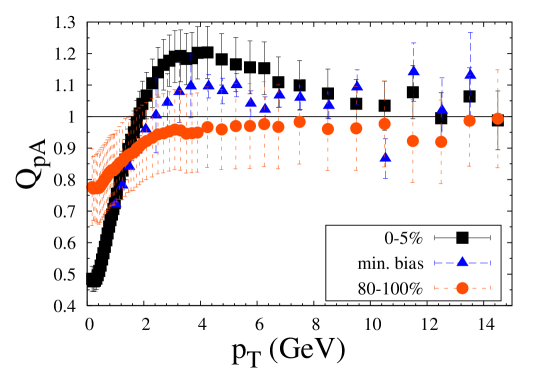
Figure 1: ALICE data Adam:2014qja for $Q_{pA}(p_{T})$ in “central”, minimum bias, and “peripheral” $p+$Pb collisions at 5.02 TeV for $p_{T}<15$ GeV. For these data sets they define centrality classes with zero degree calorimeters, and determine the number of collisions $N^{\mathrm{mult}}_{\mathrm{coll}}$ in each centrality class from the charged particle multiplicity at midrapidity.

The ALICE collaboration employed several different methods to quantify collision centrality Adam:2014qja . Their “hybrid” methods define centrality classes based on the signal of a zero degree calorimeter in the hemisphere of the nucleus which should classify events according to the number of participant nucleons. The number of binary collisions in a particular centrality class is then determined by either one of the following models:

1. the charged-particle multiplicity at mid-rapidity is proportional to the number of participants from which one obtains $N_{\mathrm{coll}}^{\mathrm{mult}}$;

2. the yield of charged high-$p_{T}$ particles at mid-rapidity is proportional to the number of binary NN collisions ($\to N^{\mathrm{high-pT}}_{\mathrm{coll}}$);

3. the target-going charged-particle multiplicity is proportional to the number of wounded target nucleons from which one obtains $N^{\mathrm{Pb-side}}_{\mathrm{coll}}$.

The ALICE collaboration denotes the nuclear modification factor in the presence of a centrality selection by ${\cal Q}_{pA}$.

Our main point is that the experimental centrality selections discussed above introduce a bias on the small-$x$ gluon configurations producing such events. For example, $pA$ events with higher than average multiplicity or transverse energy deposition not only involve more nucleon participants in the target. They also involve a biased average over the ensemble of small-$x$ gluon fields. This bias has to be accounted for also in calculations of the transverse momentum distributions. The biased average can be interpreted as reweighting of configurations,

$$\left<O\right> = \frac{\sum_{i}w_{i}O_{i}}{\sum_{i}w_{i}}~{}~{}~{}~{},~{}~{}~{}~{}w_{i}=e^{-S_{i}}~{},$$ (2)

$$\to~{}~{}\left<O\right>_{\mathrm{bias}} = \frac{\sum_{i}w^{\prime}_{i}O_{i}}{\sum_{i}w^{\prime}_{i}}~{}~{}~{}~{},~{}~{}~{}~{}w^{\prime}_{i}=w_{i}b_{i}~{}.$$ (3)

Here, $i=1\dots N$ labels field configurations, $O$ denotes an operator corresponding to a particular observable, $S_{i}$ is the action evaluated on configuration $i$, and $b_{i}$ is the configuration bias. Note that the $O_{i}$ as well as the operator averages in general are functions of transverse momentum, rapidity etc., and that the functional form of $\left<O\right>(p_{T})$ will differ from that of $\left<O\right>_{\mathrm{bias}}(p_{T})$ even when the reweighting parameters $b_{i}$ are $p_{T}$-independent numbers. The predictive power of the approach corresponds to precisely this modification of the $p_{T}$-dependence of the expectation value of the observable due to reweighting. The percentile of configurations obtained from the reweighted ensemble is given by

$$\nu_{r}=\frac{\left(\sum_{i}w^{\prime}_{i}\right)^{2}}{N\sum_{i}(w^{\prime}_{i})^{2}}~{}.$$ (4)

While we are unable to precisely replicate the centrality selections employed by the experiments, we illustrate our point within the following setting. We focus on the observable

$${\cal Q}_{pA}(k)=\frac{\left<\frac{\mathrm{d}N}{\mathrm{d}^{2}k\,\mathrm{d}y}\right>_{\mathrm{bias}}\Big{|}_{pA}}{N_{\mathrm{coll}}^{\mathrm{bias}}\,\left<\frac{\mathrm{d}N}{\mathrm{d}^{2}k\,\mathrm{d}y}\right>\Big{|}_{pp}}~{}.$$ (5)

The transverse momentum distribution in the denominator is that for minimum bias $pp$ collisions; that in the numerator corresponds to the class of $pA$ (or $pp$) collisions for a particular bias. We choose the number of hard gluons in the linear regime above the so-called “extended geometric scaling” scale, $p_{T}>Q_{gs,A}\gg Q_{s,A}$, as our “centrality” selector. (Of course, such a centrality selector can not be used by the experiments because the number of such hard particles per event is small.)

Thus, configurations of the target corresponding to a greater than average number of such high transverse momentum gluons are selected as “central” collisions. Also, we define the number of collisions for this biased sample to be given by the ratio of the number of gluons above $Q_{gs,A}$ for a heavy-ion versus a proton target:

$$N_{\mathrm{coll}}^{\mathrm{bias}}=\frac{\int\limits_{Q_{gs,A}}\mathrm{d}^{2}k\left<\frac{\mathrm{d}N}{\mathrm{d}^{2}k\,\mathrm{d}y}\right>_{\mathrm{bias}}\Big{|}_{pA}}{\int\limits_{Q_{gs,A}}\mathrm{d}^{2}k\left<\frac{\mathrm{d}N}{\mathrm{d}^{2}k\,\mathrm{d}y}\right>\Big{|}_{pp}}~{}.$$ (6)

This is motivated by one of ALICE’s methods for determining the number of collisions in a particular centrality class from the multiplicity of high transverse momentum particles, $N^{\mathrm{high-}p_{T}}_{\mathrm{coll}}$, and derives from the fact that the number of hard particles in minimum-bias collisions is proportional to $N_{\mathrm{coll}}$. However, we emphasize that here we do not consider Glauber model fluctuations of $N_{\mathrm{coll}}$ (for simplicity). Rather, here $N_{\mathrm{coll}}^{\mathrm{bias}}>N_{\mathrm{coll}}^{\mathrm{m.b.}}$ arises entirely due to the bias on the small-$x$ gluon configurations. Given this centrality selector our goal is to analyze the transverse momentum distribution below $Q_{gs,A}$ resulting from the biased average over soft gluon fields. Our main result is that, indeed, ${\cal Q}_{pA}(k)$ for a high multiplicity bias is greater than the minimum-bias $R_{pA}(k)$ at small $x$.

The importance of “color charge fluctuations” in models of the initial state for hydrodynamics of A+A collisions has been pointed out in refs. AA_color_flucs . There, one is concerned mainly with the spatial distribution of the $p_{T}$-integrated gluon (energy) density which determines the pressure gradients. Here, we focus instead on the biased nuclear modification factor which provides direct insight into the $p_{T}$ dependence of the gluon distribution functions in a reweighted JIMWLK ensemble.

We should stress that even though the bias effect on the small-$x$ fields discussed here must certainly exist, that does not imply that understanding the data would not require other, additional effects. For example, it is possible that “color reconnections” (see Sjostrand:2013cya and references therein) become more important as one selects more “central” events. Here, however, we focus on illustrating the conceptual issue of biased averages over the ensemble of small-$x$ gluon fields rather than to attempt a definitive interpretation of the data. The specific question we ask is how a multiplicity bias imposed at high transverse momentum affects the distribution of small-$x$ gluons at lower $k$.

This paper is organized as follows. In the following section we discuss basic features of biased averages over the ensemble of small-$x$ fields, and we present qualitative analytic estimates of ${\cal Q}_{pA}$. Section III presents numerical results obtained by Monte-Carlo sampling of the JIMWLK ensemble. The final section is devoted to a brief summary and discussion.

II Cross section for gluon production

To leading order in the gluon density of the projectile proton the single inclusive gluon distribution is given by CGC_pA

$$\left<E_{k}\frac{dN}{d^{3}k}\right> =\frac{1}{(2\pi)^{3}k^{2}}(\delta_{ij}\delta_{lm}+\epsilon_{ij}\epsilon_{lm})\left<\ \Omega_{ij}^{b}(\mathbf{k})\ \left[\Omega_{lm}^{b}(\mathbf{k})\right]^{*}\right>_{p,A}$$

$$=\frac{g^{2}}{(2\pi)^{3}k^{2}}(\delta_{ij}\delta_{lm}+\epsilon_{ij}\epsilon_{lm})\int{\frac{\mathrm{d}^{2}\mathbf{p}}{(2\pi)^{2}}}{\frac{\mathrm{d}^{2}\mathbf{q}}{(2\pi)^{2}}}\frac{p_{i}(k-p)_{j}}{p^{2}}\frac{q_{l}(k-q)_{m}}{q^{2}}$$

$$\quad\quad\quad\times\left<\rho_{a}^{*}(\mathbf{q})\left[W^{\dagger}(\mathbf{k}-\mathbf{q})W(\mathbf{k}-\mathbf{p})\right]_{ab}\rho_{b}(\mathbf{p})\right>_{p,A}~{}.$$ (7)

Here

$$\Omega_{ij}^{a}(\mathbf{x})=g\left[\frac{\partial_{i}}{\partial^{2}}\rho^{b}(\mathbf{x})\right]\partial_{j}W^{ab}(\mathbf{x})~{},$$ (8)

and

$$W(\mathbf{x})={\cal P}\,e^{-ig\int dx^{-}A^{+a}(x^{-},\mathbf{x})\,{T^{a}}}$$ (9)

is a Wilson line in the adjoint representation in the field of the target. The brackets in eq. (7) denote an average over the random color charge densities or soft gluon fields of both projectile and target.

For simplicity, we assume that the gluon distribution of the projectile proton can be approximated by the most likely distribution. It is straightforward, in principle, to allow for a bias on the gluon distribution of the proton along the same lines as for the nucleus. Thus, we average over all configurations of the proton projectile using

$$\left<\rho_{a}^{*}(\mathbf{q})\,\rho_{b}(\mathbf{p})\right>_{p}=\delta_{ab}\,(2\pi)^{2}\delta(\mathbf{q}-\mathbf{p})\,\mu_{p}^{2}(q^{2})~{}.$$ (10)

Then the gluon spectrum (7) becomes

$$\left<E_{k}\frac{dN}{d^{3}k}\right>=\frac{g^{2}}{(2\pi)^{3}k^{2}}\int{\frac{\mathrm{d}^{2}\mathbf{p}}{(2\pi)^{2}}}\frac{(\mathbf{k}-\mathbf{p})^{2}}{p^{2}}\,\mu^{2}_{p}(p^{2})\left<\mathrm{tr}\,W^{\dagger}(\mathbf{k}-\mathbf{p})W(\mathbf{k}-\mathbf{p})\right>_{A}~{}.$$ (11)

For high transverse momentum, $k\gg Q_{s,A}$, we can evaluate this integral in the leading logarithmic approximation:

$$\left<E\frac{dN}{d^{3}k}\right> = \frac{1}{2(2\pi)^{3}}\frac{1}{g^{2}C_{F}}\frac{Q_{s,p}^{2}}{k^{4}}\log\left(\frac{k^{2}}{Q_{s,p}^{2}}\right)\times k^{4}\left<\mathrm{tr}\,W^{\dagger}(\mathbf{k})W(\mathbf{k})\right>_{A}~{}.$$ (12)

We have introduced the saturation momentum of the proton via $Q_{s,p}^{2}=C_{F}g^{4}\mu_{p}^{2}/2\pi$ which acts as an infrared cutoff because the initial assumption that the proton be dilute does not apply below $Q_{s,p}$. At high transverse momentum the last factor on the r.h.s. of eq. (12) is approximately constant.

For intermediate transverse momenta of order $Q_{s,A}$ on the other hand we can simplify eq. (11) to

$$\left<E\frac{dN}{d^{3}k}\right> = \frac{1}{2(2\pi)^{3}}\frac{1}{g^{2}C_{F}}\frac{Q_{s,p}^{2}}{k^{2}}\log\left(\frac{Q_{s,A}^{2}}{Q_{s,p}^{2}}\right)\times k^{2}\left<\mathrm{tr}\,W^{\dagger}(\mathbf{k})W(\mathbf{k})\right>_{A}~{}.$$ (13)

Again, for $k\sim Q_{s,A}$ the last factor is approximately constant. In what follows we will restrict to $k>Q_{s,A}$, however, and work with eq. (12).

It will be useful to recall first how the nuclear suppression of

$$R_{pA}(k)=\frac{\left<\frac{\mathrm{d}N}{\mathrm{d}^{2}k\mathrm{d}y}\right>\Big{|}_{pA}}{N_{\mathrm{coll}}^{\mathrm{m.b.}}\,\left<\frac{\mathrm{d}N}{\mathrm{d}^{2}k\mathrm{d}y}\right>\Big{|}_{pp}}$$ (14)

arises in minimum bias collisions at high transverse momentum $k>Q_{s,A}$ and small $x$. This is due to the fact that the gluon distribution acquires an anomalous dimension at small $x$ which leads to “leading twist shadowing”. For detailed discussions we refer to refs. RpA ; RpA_AAKSW . At high transverse momentum we can expand the correlator of Wilson lines in eq. (12) to quadratic order in $gA^{+}$ which leads to

$$k^{4}\left<\mathrm{tr}\,W^{\dagger}(\mathbf{k})W(\mathbf{k})\right>\to g^{4}N_{c}(N_{c}^{2}-1)\,\mu^{2}(k)A_{\perp}~{}.$$ (15)

The transverse area $A_{\perp}$ in this expression is determined by the projectile proton. Also,

$$\mu^{2}(k)\simeq\mu_{0}^{2}\left(\frac{k^{2}}{Q_{s}^{2}}\right)^{1-\gamma(k)}$$ (16)

when $k>Q_{s}$ Iancu:2002aq . $\gamma(Q_{s})\equiv\gamma_{s}\simeq 0.64$ is the BFKL anomalous dimension bfkl in the presence of a saturation boundary Mueller:2002zm ; it increases logarithmically with increasing $k/Q_{s}$ and is close to its asymptotic DGLAP limit of 1 at $k^{2}\sim Q_{gs}^{2}\sim Q_{s}^{4}/\Lambda^{2}$ Levin:2000mv ; Iancu:2002tr . Note that for a nucleus $\mu_{0}^{2}\sim A^{1/3}$ is proportional to the average thickness and hence to $N_{\mathrm{coll}}^{\mathrm{m.b.}}$. Then, using eqs. (12,15) in (14) we get

$$R_{pA}(k)=\frac{\mu^{2}_{A}(k)}{N_{\mathrm{coll}}^{\mathrm{m.b.}}\,\mu^{2}_{p}(k)}\simeq(k^{2})^{\gamma_{p}(k)-\gamma_{A}(k)}\,\frac{(Q_{s,p}^{2})^{1-\gamma_{p}(k)}}{(Q_{s,A}^{2})^{1-\gamma_{A}(k)}}\simeq\left(\frac{k^{2}}{Q_{s,p}^{2}}\right)^{\gamma_{p}(k)-\gamma_{A}(k)}\,\frac{1}{(N_{\mathrm{coll}}^{\mathrm{m.b.}})^{1-\gamma_{A}(k)}}~{}.$$ (17)

For a given $k$ the anomalous dimension for the gluon distribution of the nucleus differs from that of the proton since $k/Q_{s}$ is not the same. Hence, we distinguish $\gamma_{p}(k)$ from $\gamma_{A}(k)$.

The previous equation confirms the somewhat stronger suppression of the minimum bias $R_{pA}$ for a thicker target mentioned in the introduction. Also, since $\gamma_{p}(k)>\gamma_{A}(k)$ at midrapidity it follows that $R_{pA}(k)$ increases with $k$ towards its asymptotic value of $R_{pA}(k)=1$ where both anomalous dimensions are close to 1. We emphasize that eqs. (16,17) refer to the fixed point of the small-$x$ renormalization group, i.e. to high rapidity where memory of the initial condition has been lost.

Eqs. (12,13) show that the ensemble of gluon spectra in a $pA$ collision is determined by the ensemble of adjoint dipole correlators. Rather than computing the unbiased inclusive cross section averaged over all target configurations we are interested here in performing that average subject to a constraint on the covariant gauge gluon distribution, i.e. that $g^{2}\mathrm{tr}\,A^{+}(\mathbf{q})A^{+}(-\mathbf{q})$ be equal to a given function $X(\mathbf{q})$. The distribution of functions $X(\mathbf{q})$ in the JIMWLK ensemble is described by the constraint effective potential Dumitru:2017cwt

$$e^{-V_{\mathrm{eff}}[X(\mathbf{q})]} = \int{\cal D}A^{+}(\mathbf{q})\,W_{Y}[A^{+}(\mathbf{q})]\,\delta(X(\mathbf{q})-g^{2}\mathrm{tr}\,A^{+}(\mathbf{q})\,A^{+}(-\mathbf{q}))~{}.$$ (18)

We can evaluate $V_{\mathrm{eff}}[X(\mathbf{q})]$ analytically in a Gaussian approximation where Iancu:2002aq

$$W_{Y}[A^{+}(\mathbf{q})]=e^{-S_{G}[A^{+}(\mathbf{q})]}~{}~{}~{}~{}~{},~{}~{}~{}~{}~{}S_{G}[A^{+}(\mathbf{q})] = \int{\frac{\mathrm{d}^{2}\mathbf{q}}{(2\pi)^{2}}}\,q^{4}\,\frac{\mathrm{tr}\,A^{+}(\mathbf{q})\,A^{+}(-\mathbf{q})}{g^{2}\mu^{2}(q^{2})}~{}.$$ (19)

$\mu^{2}(q^{2})$ evolves with rapidity but we shall leave this dependence implicit. With the Gaussian action for $A^{+}$ one obtains (see ref. Dumitru:2017cwt for details)

$$V_{\mathrm{eff}}[X(\mathbf{q})] = \int\frac{\mathrm{d}^{2}\mathbf{q}}{(2\pi)^{2}}\left[\frac{q^{4}}{g^{4}\mu^{2}(q)}X(\mathbf{q})-\frac{1}{2}A_{\perp}N_{c}^{2}\log X(\mathbf{q})\right]~{}.$$ (20)

The extremal configuration is determined by $\delta V_{\mathrm{eff}}[X(q)]/\delta X(\ell)=0$ to be

$$X_{s}(\ell)=\frac{1}{2}N_{c}^{2}A_{\perp}\frac{g^{4}\mu_{A}^{2}(\ell)}{\ell^{4}}~{}.$$ (21)

This is equal to $\left<X(\ell)\right>$ up to terms of order ${N_{c}}^{0}$. The partition sum is

$$Z=\int{\cal D}X(\mathbf{q})\,e^{-V_{\mathrm{eff}}[X(\mathbf{q})]}~{},$$ (22)

and the unbiased expectation value of an observable $O[g^{2}\mathrm{tr}\,|A^{+}(\mathbf{q})|^{2}]$ can be written as

$$\left<O\right>=\frac{1}{Z}\int{\cal D}X(\mathbf{q})\,e^{-V_{\mathrm{eff}}[X(\mathbf{q})]}\,O[X(\mathbf{q})]~{}.$$ (23)

Below, integrals over $X(\mathbf{q})$ are understood to be normalized by $1/Z$ as appropriate. A biased average of $O$ can be obtained by restricting the set of functions $X(\mathbf{q})$ that one integrates over in eq. (23). More generally, one may reweight like in eq. (3) by letting $\exp(-V_{\mathrm{eff}}[X(\mathbf{q})])\to\exp(-V_{\mathrm{eff}}[X(\mathbf{q})])\,b[X(\mathbf{q})]$. For

$$b[X]=\exp\left(\int\mathrm{d}^{2}{\mathbf{q}}\,t(\mathbf{q})X(\mathbf{q})\right)~{},$$ (24)

in particular, $Z[t]=\left<1\right>_{t}$ is a generating functional for the correlation functions of $X(\mathbf{q})$:

$$\frac{1}{Z}\frac{\delta^{n}Z[t]}{\delta t(\mathbf{k}_{1})\cdots\delta t(\mathbf{k}_{n})}\Bigr{|}_{t\equiv 0}=\left<X(\mathbf{k}_{1})\cdots X(\mathbf{k}_{n})\right>~{}.$$ (25)

II.1 The distribution of functions $\mathrm{tr}\,W^{\dagger}(\mathbf{k})W(\mathbf{k})$ at order $(gA^{+})^{2}$

We now determine the distribution of the functions $\mathrm{tr}\,W^{\dagger}(\mathbf{k})W(\mathbf{k})$. To do so, we expand the Wilson lines in powers of the covariant gauge field $gA^{+}$. To order $(gA^{+})^{2}$,

$$\left<\mathrm{tr}\,W^{\dagger}(\mathbf{k}-\mathbf{p})W(\mathbf{k}-\mathbf{p})\right> = -\frac{g^{4}N_{c}(N_{c}^{2}-1)A_{\perp}}{(2\pi)^{2}}\int\mathrm{d}^{2}\mathbf{r}\,e^{-i(\mathbf{k}-\mathbf{p})\cdot\mathbf{r}}\int\frac{\mathrm{d}^{2}\mathbf{s}}{s^{4}}\mu^{2}_{A}(s)\left(1-e^{i\mathbf{s}\cdot\mathbf{r}}\right)$$ (27)

$$\times\int{\cal D}X(\mathbf{q})\,e^{-V_{\mathrm{eff}}[X(q)]}\,\frac{X(\mathbf{s})}{X_{s}(s)}$$

$$=g^{4}N_{c}(N_{c}^{2}-1)A_{\perp}\int\frac{\mathrm{d}^{2}\mathbf{s}}{s^{4}}\left[\delta(\mathbf{k}-\mathbf{p}-\mathbf{s})-\delta(\mathbf{k}-\mathbf{p})\right]\,\mu^{2}_{A}(s)\int{\cal D}X(\mathbf{q})\,e^{-V_{\mathrm{eff}}[X(q)]}\,\frac{X(\mathbf{s})}{X_{s}(s)}~{}.$$

By inspection of eq. (11) the “tadpole” subtraction $\sim\delta(\mathbf{k}-\mathbf{p})$ does not contribute and can be dropped:

$$\left<\mathrm{tr}\,W^{\dagger}(\mathbf{k}-\mathbf{p})W(\mathbf{k}-\mathbf{p})\right>\to\frac{g^{4}N_{c}(N_{c}^{2}-1)}{(\mathbf{k}-\mathbf{p})^{4}}\,\mu^{2}_{A}(|\mathbf{k}-\mathbf{p}|)A_{\perp}\int{\cal D}X(\mathbf{q})\,e^{-V_{\mathrm{eff}}[X(q)]}\,\frac{X(\mathbf{k}-\mathbf{p})}{X_{s}(|\mathbf{k}-\mathbf{p}|)}~{}.$$ (28)

Also, if the distribution $e^{-V_{\mathrm{eff}}[X(q)]}$ of functions $X(\mathbf{q})$ is assumed to be infinitely strongly peaked about $X_{s}(q)$ then the integral over $X(\mathbf{q})$ is equal to 1 (recall that we suppress the $Z^{-1}$ normalization factor for ease of notation), and we recover eq. (15) from above.

Since we expanded the product of Wilson lines to leading non-trivial power of $A^{+}$ only, we must use eq. (28) for the high-$k$ gluon spectrum. Hence, eq. (12) now reads

$$\left<E\frac{dN}{d^{3}k}\right>_{\mathrm{high-}k} = \frac{g^{2}N_{c}^{2}\mu^{2}_{A}(k)A_{\perp}}{(2\pi)^{3}}\frac{Q_{s,p}^{2}}{k^{4}}\log\left(\frac{k^{2}}{Q_{s,p}^{2}}\right)\int{\cal D}X(\mathbf{q})\,e^{-V_{\mathrm{eff}}[X(q)]}\,\frac{X(\mathbf{k})}{X_{s}(k)}~{}.$$ (29)

To understand qualitatively the effect due to the bias towards functions $X(\mathbf{q})$ corresponding to a greater than average number of hard gluons we assume that the saddle point of the reweighted (biased) ensemble is shifted to

$$\frac{X(\mathbf{q})}{X_{s}(q)} = 1+\eta_{0}\left(\frac{{q_{0}}^{2}}{q^{2}}\right)^{a}\,\Theta(Q^{2}-q^{2})\,\Theta(q^{2}-Q^{2}_{s,A})~{},~{}~{}~{}~{}~{}~{}~{}~{}~{}(a,\eta_{0}\geq 0).$$ (30)

Such a shift could be obtained by reweighting with

$$\log b[X]\simeq\frac{1}{2}A_{\perp}N_{c}^{2}\,\eta_{0}\int\limits_{Q_{\mathrm{gs}}^{2}}^{Q^{2}}\frac{\mathrm{d}^{2}\mathbf{\ell}}{(2\pi)^{2}}\frac{X(\ell)-X_{s}(\ell)}{X_{s}(\ell)}\left(\frac{{q_{0}}^{2}}{\ell^{2}}\right)^{a}+{\cal O}\left({\eta_{0}}^{2}\right)~{}.$$ (31)

While this functional reweights configurations based only on the number of gluons above the extended geometric scaling scale $Q_{\mathrm{gs}}$, we shall see in sec. III that, in fact, a spectral shape like in eq. (30) emerges automatically all the way down to scales of order $Q_{s,A}$.

Our trial function (30) increases the number of gluons in the transverse momentum range between $Q_{s,A}$ and $Q$. The parameter $\eta_{0}$ corresponds to the amplitude of the enhancement, and $Q\sim Q_{gs,A}$ determines how far in transverse momentum it extends. $q_{0}$ is some fixed transverse momentum scale, for instance $Q_{s,p}(Y=0)$. Obviously, ${q_{0}}^{2a}$ could be absorbed into $\eta_{0}$ but writing $X(\mathbf{q})$ in the form (30) appears clearer.

Such $X(\mathbf{q})$ comes with a penalty action of

$$V_{\mathrm{eff}}[X(q)]\simeq\frac{1}{8\pi}N_{c}^{2}A_{\perp}\,q_{0}^{2}\,\eta_{0}\times\begin{cases}\frac{1}{1-a}\left(\frac{Q^{2}}{q_{0}^{2}}\right)^{1-a}&(0\leq a<1)~{},\\ \log\frac{Q^{2}}{Q_{s,A}^{2}}&(a=1)~{}.\end{cases}$$ (32)

Without reweighting it is suppressed by a relative probability

$$p_{r}=\frac{w[X(\mathbf{q})]}{w[X_{s}(q)]}=e^{-V_{\mathrm{eff}}[X(q)]}~{}~{}~{}~{}~{}~{},~{}~{}~{}~{}~{}w[X_{s}(q)]=\frac{1}{Z}~{}.$$ (33)

Hence, a nearly uniform distortion of the gluon distribution ($a\sim 0$) is highly suppressed since $V_{\mathrm{eff}}$ is proportional to a power of $Q^{2}$. For $a>1$, on the other hand, the penalty action is small but such deviations from the average gluon distribution do not increase the multiplicity above $Q_{gs,A}$ significantly, and therefore they do not dominate the configuration bias. Therefore, from now on we take $a=1$ for illustration. Note the weak dependence of $V_{\mathrm{eff}}[X(q)]$ on the lower limit $Q_{s,A}$ of the distortion of the gluon distribution for $a\leq 1$. Thus, adding gluons with transverse momenta all the way down to $Q_{s,A}$ does not come at a high price.

Given a suppression factor (relative weight) $p_{r}$ we can eliminate one of the parameters of the trial function, for example

$$\eta_{0}\,q_{0}^{2}\simeq\frac{8\pi\log p_{r}^{-1}}{N_{c}^{2}A_{\perp}\log\frac{Q^{2}}{Q_{s,A}^{2}}}~{}.$$ (34)

Next, to determine $N_{\mathrm{coll}}[\eta]$ we integrate eq. (29) over $k>Q_{gs,A}$ for the trial function (30) with $a=1$:

$$\frac{dN_{pA}}{dy}\Big{|}_{\overset{\mathrm{high\,}k}{\mathrm{high~{}mult}}} = \frac{\pi g^{2}N_{c}^{2}\mu^{2}_{0,A}A_{\perp}}{(2\pi)^{3}}\frac{Q_{s,p}^{2}}{Q_{gs,A}^{2}}\left[1+\frac{\eta_{0}}{2}\frac{q_{0}^{2}}{Q_{gs,A}^{2}}\right]\log\left(\frac{Q_{gs,A}^{2}}{Q_{s,p}^{2}}\right)~{}.$$ (35)

We approximate $\gamma_{\mathrm{DGLAP}}\simeq 1$. For a proton target the multiplicity above $k=Q_{gs,A}$, on average over configurations, is

$$\left<\frac{dN_{pp}}{dy}\right>_{\mathrm{high\,}k} = \frac{\pi g^{2}N_{c}^{2}\mu^{2}_{0,p}A_{\perp}}{(2\pi)^{3}}\frac{Q_{s,p}^{2}}{Q_{gs,A}^{2}}\log\left(\frac{Q_{gs,A}^{2}}{Q_{s,p}^{2}}\right)~{}.$$ (36)

Hence,

$$N_{\mathrm{coll}}\Big{|}_{\mathrm{high~{}mult}}=\frac{\mu^{2}_{0,A}}{\mu^{2}_{0,p}}\left[1+\frac{\eta_{0}q_{0}^{2}}{2Q_{gs,A}^{2}}\right]~{}.$$ (37)

Finally, to obtain ${\cal Q}_{pA}(k)$ we divide the gluon spectrum for a heavy-ion target from eq. (29), for the specific $X(q)$ written in eq. (30), by $N_{\mathrm{coll}}\big{|}_{\mathrm{high~{}mult}}$ and by the average gluon spectrum for a proton target:

$${\cal Q}_{pA}(k)=\frac{1+\eta_{0}\left(\frac{q_{0}^{2}}{k^{2}}\right)}{1+\frac{\eta_{0}}{2}\frac{q_{0}^{2}}{Q_{gs,A}^{2}}}\frac{(k^{2})^{\gamma_{p}(k)-\gamma_{A}(k)}}{Q_{s,A}^{2-2\gamma_{A}(k)}Q_{s,p}^{2\gamma_{p}(k)-2}}=\frac{1+\eta_{0}\left(\frac{q_{0}^{2}}{k^{2}}\right)}{1+\frac{\eta_{0}}{2}\frac{q_{0}^{2}}{Q_{gs,A}^{2}}}\,R_{pA}(k)~{}.$$ (38)

In the second step we used the result for $R_{pA}(k)$ written in eq. (17) above. For $k\sim Q_{gs,A}$ we have ${\cal Q}_{pA}(k)\simeq 1$ since both anomalous dimensions are close to 1, just like for minimum bias collisions discussed in eq. (17). In fact, ${\cal Q}_{pA}(k)$ as we define it asymptotically drops below $R_{pA}$ but only slightly, since from eq. (34) it follows that $\eta_{0}q_{0}^{2}/Q^{2}_{gs,A}\ll 1$. In any case, the most interesting regime to us is $k<Q_{gs}$.

The key point is that by selecting events with a slightly modified spectrum at high transverse momentum, $k\sim Q_{gs,A}$, we study the modification at lower transverse momentum well below $Q_{gs,A}$. In this regime ${\cal Q}_{pA}(k)-R_{pA}(k)$ increases with decreasing $k$. With $\eta_{0}$ from eq. (34),

$${\cal Q}_{pA}(k) \simeq \left(1+\frac{8\pi\log p_{r}^{-1}}{N_{c}^{2}A_{\perp}k^{2}\log\frac{Q^{2}}{Q^{2}_{s,A}}}\right)\,R_{pA}(k)~{}.$$ (39)

To simplify this expression we have assumed that $\eta_{0}q_{0}^{2}/Q^{2}_{gs,A}\ll 1$. Note that

$$\frac{8\pi\log p_{r}^{-1}}{N_{c}^{2}A_{\perp}k^{2}\log\frac{Q^{2}}{Q^{2}_{s,A}}}\,R_{pA}(k)$$ (40)

can also be interpreted as the difference of ${\cal Q}_{pA}(k)$, $k$ in the range $Q_{s,A}\ll k\ll Q_{gs,A}$, for two classes of events with relative probability $p_{r}$. Also, we find that ${\cal Q}_{pA}(k)-R_{pA}(k)$ increases with decreasing area of the projectile. Away from midrapidity and towards the hemisphere of the nucleus ${\cal Q}_{pA}(k)-R_{pA}(k)$ should increase, and vice versa.

Thus, we have shown in this section that it is possible, in principle, that a bias on configurations with slightly enhanced gluon density in the target at high transverse momentum, and correspondingly slightly higher $N_{\mathrm{coll}}$, exhibits the features seen in the data. Namely, that ${\cal Q}_{pA}(k)\simeq 1$ at $k\sim Q_{gs,A}$ where the anomalous dimension is close to its DGLAP limit, while ${\cal Q}_{pA}(k)-R_{pA}(k)$ then increases with decreasing $k$.

II.2 $\left<\mathrm{tr}\,W^{\dagger}(x)W(y)\right>$ to all orders in $(gA^{+})^{4}$

For completeness, in this section we provide the resummed expression for $\left<\mathrm{tr}\,W^{\dagger}(x)W(y)\right>$, to all orders in $A^{+}$. We did not require the all-order expression for our considerations above because we restricted to transverse momenta in the linear regime above the saturation scale.

We first compute explicitly the contribution to $\left<\mathrm{tr}\,W^{\dagger}(\mathbf{x})W(\mathbf{y})\right>$ at fourth order in $gA^{+}$:

$$\frac{1}{2}g^{8}N_{c}^{2}(N_{c}^{2}-1)\int{\cal D}X(\mathbf{q})\,e^{-V_{\mathrm{eff}}[X(\mathbf{q})]}\left(\int\frac{\mathrm{d}^{2}\mathbf{s}}{(2\pi)^{2}}\,\frac{\mu^{2}(s)}{s^{4}}\left(1-e^{i\mathbf{s}\cdot\mathbf{r}}\right)\frac{X(\mathbf{s})}{X_{s}(s)}\right)^{2}~{},$$ (41)

where $\mathbf{r}=\mathbf{y}-\mathbf{x}$. This is recognized as one half the square of the contribution at order $(A^{+})^{2}$ written in eq. (27), except for the overall factor of $(N_{c}^{2}-1)$, a Fourier transform w.r.t. $\mathbf{r}$, and an integration over transverse impact parameter space. This is a consequence of the ordering in $x^{-}$ which generalizes to all orders in $A^{+}$ so that

$$\left<\frac{1}{N_{c}^{2}-1}\mathrm{tr}\,W^{\dagger}(\mathbf{x})W(\mathbf{y})\right>=\int{\cal D}X(\mathbf{q})\,e^{-V_{\mathrm{eff}}[X(\mathbf{q})]}\,\exp\left(-g^{4}N_{c}\int\frac{\mathrm{d}^{2}\mathbf{s}}{(2\pi)^{2}}\,\frac{\mu^{2}(s)}{s^{4}}\left(1-e^{i\mathbf{s}\cdot\mathbf{r}}\right)\frac{X(\mathbf{s})}{X_{s}(s)}\right)~{}.$$ (42)

With $X_{s}(s)$ from eq. (21) we can also write this as

$$\left<\frac{1}{N_{c}^{2}-1}\mathrm{tr}\,W^{\dagger}(\mathbf{x})W(\mathbf{y})\right>=\int{\cal D}X(\mathbf{q})\,e^{-V_{\mathrm{eff}}[X(\mathbf{q})]}\,\exp\left(-\frac{2}{N_{c}A_{\perp}}\int\frac{\mathrm{d}^{2}\mathbf{s}}{(2\pi)^{2}}\left(1-e^{i\mathbf{s}\cdot\mathbf{r}}\right)X(\mathbf{s})\right)~{}.$$ (43)

For the trial functions (30) we obtain

$$\frac{1}{N_{c}^{2}-1}\mathrm{tr}\,W^{\dagger}(\mathbf{x})W(\mathbf{y})\Big{|}_{X(s)=\mathrm{eq.\,}(\ref{eq:trialX})}\sim\exp\left(-\frac{1}{4}\frac{C_{A}}{C_{F}}\frac{1}{2-2\gamma}\left(r^{2}Q_{s,A}^{2}\right)^{\gamma}-\frac{1}{8}\frac{C_{A}}{C_{F}}\frac{\eta_{0}}{a+\gamma-1}Q_{s,A}^{2}r^{2}\frac{q_{0}^{2a}}{Q_{s,A}^{2a}}\right)$$ (44)

if $r^{2}Q^{2}\ll 1$; and

$$\frac{1}{N_{c}^{2}-1}\mathrm{tr}\,W^{\dagger}(\mathbf{x})W(\mathbf{y})\Big{|}_{X(s)=\mathrm{eq.\,}(\ref{eq:trialX})}\sim\exp\left(-\frac{1}{4}\frac{C_{A}}{C_{F}}\frac{1}{2-2\gamma}\left(r^{2}Q_{s,A}^{2}\right)^{\gamma}-\frac{1}{8}\frac{C_{A}}{C_{F}}\frac{\eta_{0}}{a+\gamma-1}q_{0}^{2a}Q_{s,A}^{2\gamma}(r^{2})^{\gamma+a}\right)~{}.$$ (45)

if $r^{2}Q^{2}\gg 1$. Recall that $Q^{2}\gg Q_{s,A}^{2}$ denotes the maximum transverse momentum for the distortion of the gluon distribution due to the bias. To arrive at the expressions above we have assumed that $\gamma$ is constant, that $a+\gamma>1$, and that $r$ is much less than any non-perturbative infrared cutoff such as the radius of the proton. Also, throughout the manuscript $Q_{s}^{2}$ denotes the saturation scale for a fundamental dipole which is why the factor $C_{A}/C_{F}\simeq 2$ appears. The factor $\eta_{0}q_{0}^{2a}$ can be expressed in terms of the suppression probability $p_{r}$ as explained above. For a nearly fixed $r$, say $r\sim 1/Q_{s,A}$, the correction in the exponent of eq. (45) effectively corresponds to a shift of the saturation scale. However, this interpretation does not apply in general since the correction due to the bias involves a different power of $r^{2}$ than the unbiased average dipole correlator.

III Numerical results for the functional distribution of the correlator of adjoint Wilson lines from JIMWLK evolution

In this section we show results of numerical Monte-Carlo simulations of $\mathrm{tr}\,W^{\dagger}(\mathbf{q})W(-\mathbf{q})$. We generate random color charge configurations of the target on a large lattice according to the action of the McLerran-Venugopalan model MV from which we determine the covariant gauge field $A^{+}$. These are then evolved to rapidity $Y>0$ by solving the leading order B-JIMWLK renormalization group equations balitsky ; jimwlk at fixed coupling. The saturation scale $Q_{s}(Y)$ is determined implicitly from the forward scattering amplitude of a fundamental dipole: ${\cal N}_{Y}(r=\sqrt{2}/Q_{s})=1-1/\sqrt{e}$. Note that ${\cal N}_{Y}(r)$ is averaged over all field configurations.

We employ a simple reweighting procedure, taking $b_{i}=1$ for a subset of 5% of configurations with the most gluons at high $p_{T}>Q_{\mathrm{gs}}$, and $b_{i}=0$ for the rest. We do not impose any constraints such as eq. (30) on the spectral shape of the gluon distribution in this sample, neither below nor above $Q_{\mathrm{gs}}$.

For a heavy ion versus a proton target we set the ratio of initial saturation scales by default to $Q^{2}_{s,A}(Y=0)/Q^{2}_{s,p}(Y=0)=\mu^{2}_{A}/\mu^{2}_{p}=6$. This corresponds to the thickness of the nucleus relative to a nucleon. As already mentioned above we do not attempt to include Glauber model fluctuations of $N_{\mathrm{coll}}$ but focus, instead, on the distribution of functions $\mathrm{tr}\,W^{\dagger}(\mathbf{q})W(-\mathbf{q})$ over the MV or JIMWLK ensembles at fixed $\mu^{2}_{A}$. However, for comparison we shall also show results for $\mu^{2}_{A}/\mu^{2}_{p}=2$ and 1.

The correlator of adjoint Wilson lines includes an integral over the transverse overlap $A_{\perp}$ of projectile and target since

$$\mathrm{tr}\,W^{\dagger}(\mathbf{k})W(\mathbf{k})=\int_{A_{\perp}}{\mathrm{d}^{2}\mathbf{b}}\int{\mathrm{d}^{2}\mathbf{r}}\,e^{-i\mathbf{k}\cdot\mathbf{r}}\,\mathrm{tr}\,W^{\dagger}\left(\mathbf{b}+\frac{\mathbf{r}}{2}\right)\,W\left(\mathbf{b}-\frac{\mathbf{r}}{2}\right)~{}.$$ (46)

The numerical computations of $\mathrm{tr}\,W^{\dagger}(\mathbf{k})W(\mathbf{k})$ shown below are performed on a large lattice and we need to explicitly restrict the integration over $d^{2}\mathbf{b}$ to the area of a proton. To do so, in the numerical computations presented in this section we take

$$W^{G}_{ab}(\mathbf{k}) = \int d^{2}\mathbf{x}\,e^{-i\mathbf{k}\cdot\mathbf{x}}\,e^{-x^{2}/2B}\,W_{ab}(\mathbf{x})~{},$$ (47)

$$\mathrm{tr}\,W^{\dagger}(\mathbf{k})W(\mathbf{k}) \to \mathrm{tr}\,W^{G\dagger}(\mathbf{k})\,W^{G}(\mathbf{k})~{}.$$ (48)

We shall focus on transverse momenta $k\gg 1/\surd{B}$ and so the dominant dipole size $r$ in eq. (46) is set by $\sim 1/k$ and not by $\surd{B}$. Rather, $B<\infty$ restricts the endpoints of the dipole to within a patch of area $\sim 2\pi B$ around $\mathbf{b}=0$. Our default value is $\sqrt{B}\,Q_{s,p}(Y=0)=\sqrt{2/3}$. (In physical units this translates to $\sqrt{B}\approx 0.33$ fm and $2\pi B\approx 0.67$ fm² if $Q_{s,p}(Y=0)\approx 0.5$ GeV.)

Our goal is to determine numerically the function

$${\cal Q}(k)=\frac{\left<\mathrm{tr}\,W^{G\dagger}(\mathbf{k})W^{G}(\mathbf{k})\Big{|}_{A}\right>_{\mathrm{bias}}}{N_{\mathrm{coll}}^{\mathrm{bias}}\left<\mathrm{tr}\,W^{G\dagger}(\mathbf{k})W^{G}(\mathbf{k})\Big{|}_{p}\right>}~{}.$$ (49)

The Wilson lines in the numerator correspond to the field of a heavy ion while those in the denominator correspond to a proton. The corresponding field configurations differ by the choice of initial saturation scales, $Q^{2}_{s,A}(Y=0)/Q^{2}_{s,p}(Y=0)=\mu^{2}_{A}/\mu^{2}_{p}>1$, as already mentioned above. Also, in the denominator we average over all configurations while the average in the numerator is biased towards “high multiplicity” configurations as follows.

To each configuration we associate a “number of gluons” in the linear regime of high transverse momenta,

$$N_{g}=Q_{s,p}^{2}(Y)\int\limits_{Q_{\mathrm{gs}}(Y)}{\mathrm{d}^{2}\mathbf{k}}\,\mathrm{tr}\,W^{G\dagger}(\mathbf{k})\,W^{G}(\mathbf{k})~{}.$$ (50)

This is similar to the integral of eq. (12) over $\mathbf{k}$, up to a logarithm. Also, we take $Q_{\mathrm{gs}}(Y)=\sqrt{3}\frac{Q^{2}_{s,A}(Y)}{Q_{s,p}(Y=0)}$. Note that the lower limit of the integral over $\mathbf{k}$ has to increase in proportion to $Q^{2}_{s,A}(Y)$ in order to avoid the regime where the anomalous dimension differs significantly from its DGLAP limit.

$\left<\cdots\right>_{\mathrm{bias}}$ in eq. (49) corresponds to an average over the subset of configurations with the highest gluon multiplicity (for example, the 5% percentile). Also, we define the “number of binary collisions”, used in eq. (49), for this subset of configurations via

$$N_{\mathrm{coll}}^{\mathrm{bias}}=\frac{\left<N_{g}\Big{|}_{A}\right>_{\mathrm{bias}}}{\left<N_{g}\Big{|}_{p}\right>}~{}.$$ (51)

We emphasize that this quantity is still of order $A^{1/3}$, proportional to the thickness of the nucleus, because the gluon distributions for all configurations from the MV/JIMWLK ensembles are proportional to $A^{1/3}$. In the absence of the multiplicity bias $N_{\mathrm{coll}}\approx Q_{s,A}^{2}(Y)/Q_{s,p}^{2}(Y)$ equals the ratio of the squared saturation momenta. ${\cal Q}(k)$ then simply corresponds to the scaled ratio of the “minimum bias” gluon distributions of a heavy ion target and a proton.

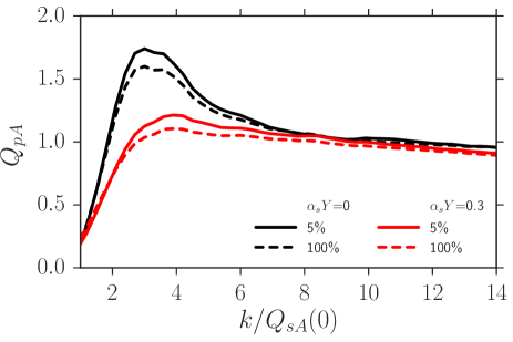
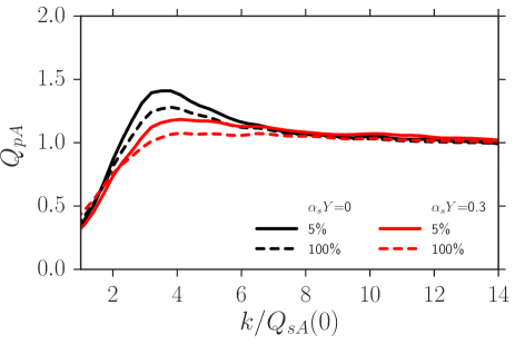
Figure 2: The ratio ${\cal Q}_{pA}(k)$ of $\left<\mathrm{tr}\,W^{\dagger}(k)W(k)\right>$ for a heavy-ion to a proton target normalized by $N_{\mathrm{coll}}$ as defined in eqs. (50,51). This is analogous to the ratio of spectra of gluons produced in $pA$ vs. $pp$ collisions divided by $N_{\mathrm{coll}}$. From top to bottom the pairs of curves correspond to the MV model initial condition at $Y=0$, and to the JIMWLK ensemble at $\alpha_{s}Y=0.3$, respectively. The dashed curves refer to the unbiased nuclear target correlator ($R_{pA}$) while the solid curves correspond to subsamples of 5% of configurations with the most gluons at high $k>Q_{gs}(Y)$. For the figure on the left (right) the nucleus is assumed to have a thickness of $\mu_{A}^{2}/\mu_{p}^{2}=6$ (2) nucleons.

Our result for ${\cal Q}_{pA}(k)$ for a target with a thickness of 6 nucleons is shown in fig. 2 (left). The magnitude of the minimum bias “Cronin peak” at $Y=0$ is similar to that obtained from the correlator of fundamental Wilson lines RpA_AAKSW . With increasing rapidity we observe the well-known overall suppression of the nuclear modification factor. Our main interest here is in the effect of the multiplicity bias on this ratio. Indeed, we observe that a bias on high hard particle multiplicity drives ${\cal Q}_{pA}(k)$ up. Also, the slope beyond the peak decreases with increasing evolution rapidity which agrees with the arguments presented in sec. II.1. It is not straightforward to match the evolution “time” $\alpha_{s}Y$ in these fixed coupling computations to a collision energy. However, we note that the unbiased ratio at $\alpha_{s}Y=0.3$ is quite similar to the measured $R_{pA}(k)$ in minimum-bias p+Pb collisions at 5 TeV. At that rapidity then, the enhancement of ${\cal Q}_{pA}(k)$ for the 5% percentile relative to $R_{pA}(k)$ is also not too different from the ALICE data shown in fig. 1. Thus, we find that it is important to account for the multiplicity bias on the small-$x$ gluon field ensemble average.

Fig. 2 (right) shows ${\cal Q}_{pA}(k)$ for a target with a thickness of only 2 nucleons. At the initial rapidity this generates a significantly smaller “Cronin peak” than the 6 nucleon target, as expected. On the other hand, JIMWLK evolution leads to a rather weak dependence on the thickness of the target: the dashed lines corresponding to $\alpha_{s}Y=0.3$ in the two panels of fig. 2 do not differ by much. In fact, selecting the 5% “most central” configurations enhances the peak at $\alpha_{s}Y=0.3$ at least as much as increasing the thickness from 2 to 6 nucleons. This illustrates again that at high energy the centrality selection not only selects events with more target nucleons but that it also biases significantly the average over small-$x$ gluon field configurations.

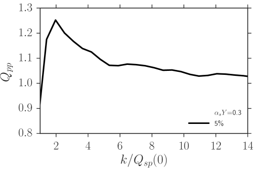
Figure 3: The ratio ${\cal Q}_{pp}(k)$ of $\left<\mathrm{tr}\,W^{\dagger}(k)W(k)\right>$ for central to minimum-bias $pp$ collisions normalized by $N_{\mathrm{coll}}$ as defined in eqs. (50,51). The curve corresponds to the JIMWLK ensemble at $\alpha_{s}Y=0.3$.

The bias due to selection of a high hard particle multiplicity modifies the observed gluon distribution even in $pp$ collisions. This is shown in fig. 3 which corresponds to $\mu^{2}_{A}/\mu^{2}_{p}=1$. Hence, the unbiased $R_{pA}(k)=1$ at any rapidity. However, at $\alpha_{s}Y=0.3$, when we select configurations with a higher than average gluon multiplicity at $k>Q_{gs}(Y)$ that generates an enhancement of ${\cal Q}_{pp}(k)$ relative to the unbiased ensemble, and a “Cronin peak” at $k/Q_{s,p}(0)\simeq 2$. In practice, this peak occurs at rather low transverse momentum and may be difficult to observe. However, beyond the peak we clearly observe ${\cal Q}_{pp}(k)-1>0$ and that, again, it falls off approximately like $1/k^{2\nu}$ with $\nu=0.6\pm 0.1$.

So far we have identified the area $A_{\perp}$ over which we integrate the Fourier transform of $\left<\mathrm{tr}\,W^{\dagger}(x)W(y)\right>$ with the area of the projectile proton, and used $\sqrt{B}=\sqrt{2/3}/Q_{s,p}(Y=0)\approx 0.33$ fm, $2\pi B\approx 0.67$ fm². We now explore the dependence of the biased nuclear modification factor ${\cal Q}_{pA}(k)$ on the area $A_{\perp}=2\pi B$. We expect that the ensemble of $\mathrm{tr}\,W^{\dagger}(k)W(k)$ probes larger deviations from the average as the area decreases.

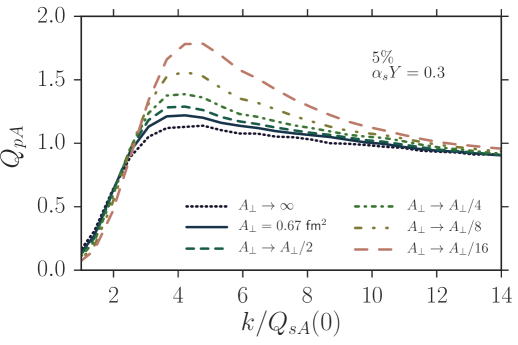
Figure 4: The ratio ${\cal Q}_{pA}(k)$ of $\left<\mathrm{tr}\,W^{\dagger}(k)W(k)\right>$ at $\alpha_{s}Y=0.3$ for the 0-5% centrality class. The target has a thickness of $\mu_{A}^{2}/\mu_{p}^{2}=6$ nucleons. From bottom to top the curves correspond to an area $A_{\perp}=2\pi B\to\infty$, to the default $2\pi B=4\pi/(3Q_{s,p}^{2}(Y=0))\approx 0.67$ fm², and to the default rescaled by 1/2, 1/4, 1/8, and 1/16, respectively.

In fig. 4 we show ${\cal Q}_{pA}(k)$ for the 5% centrality percentile for different areas. Taking $B\to\infty$ gives ${\cal Q}_{pA}(k)$ close to the minimum bias nuclear modification factor since the average over an infinite transverse area converges toward the average over many independent configurations, i.e. to no bias. For decreasing area one observes, indeed, a stronger bias due to our “centrality” selection, and a more pronounced Cronin peak. Ref Frankfurt:2003td suggested that events in which a very hard dijet ($p_{T}\sim 100$ GeV) is produced may correspond to configurations of the proton where its small-$x$ gluons occupy a smaller transverse area. Alternatively, one may tag on the presence of a $Z$-boson atlas-Z . If a high-$Q^{2}$ trigger indeed selects more compact configurations then it would be very interesting to analyze ${\cal Q}_{pA}(k)$ for such event samples.

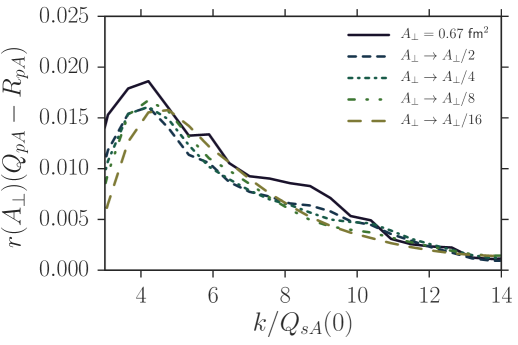
Figure 5: ${\cal Q}_{pA}(k)$ for the 0-5% centrality class minus the minimum bias $R_{pA}(k)$, both at rapidity $\alpha_{s}Y=0.3$. The target has a thickness of $\mu_{A}^{2}/\mu_{p}^{2}=6$ nucleons. We rescale the vertical axis by a factor of $r(A_{\perp})\sim{A_{\perp}}^{\nu}$ with $\nu\approx 0.6\pm 0.1$.

To exhibit the scaling of ${\cal Q}_{pA}(k)-R_{pA}(k)$ with the transverse area more clearly in fig. 5 we multiply this quantity by

$$r(A_{\perp})=\left(\frac{A_{\perp}}{A_{\perp}^{\mathrm{def}}}\right)^{\nu}~{}.$$ (52)

Here, $A_{\perp}^{\mathrm{def}}=2\pi B\approx 0.67$ fm² represents our default. For $\nu=0.6\pm 0.1$ we observe approximate scaling in that the curves corresponding to different areas are mapped onto each other. Thus, for $A_{\perp}$ not very much smaller than our default proton projectile the difference of ${\cal Q}_{pA}(k)$ and $R_{pA}(k)$ scales approximately like $\sim 1/{A_{\perp}}^{0.6}$. Furthermore, beyond the peak ${\cal Q}_{pA}(k)-R_{pA}(k)$ falls off like $\sim(k^{2})^{-0.6}$. In all,

$${\cal Q}_{pA}(k)-R_{pA}(k)\sim\left(A_{\perp}k^{2}\right)^{-0.6\pm 0.1}~{}.$$ (53)

IV Summary and Outlook

The nuclear modification factor $R_{pA}(p_{\perp})$ in proton-nucleus collisions provides insight into the gluon distribution of a dense target. It is expected to exhibit leading twist shadowing for transverse momenta below the so-called extended geometric scaling scale $Q_{gs}(Y)$. This is due to the fact that the small-$x$ gluon distribution acquires an anomalous dimension $\gamma_{s}<\gamma_{\mathrm{DGLAP}}$. Furthermore, one expects a stronger suppression of $R_{pA}(p_{\perp})$ with increasing thickness of the target.

One may also study the nuclear modification factor in a subclass of $pp$ and $pA$ events, for example in “central” collisions as defined by a suitable centrality selection. In $pA$ collisions this would select events where the projectile proton suffers an inelastic interaction with a greater than average number of target nucleons. However, such a selection of events also introduces a bias on the ensemble of gluon distribution functions of the target over which one averages.

In this paper we have provided first analytical and numerical studies of the biased nuclear (or proton) modification factor ${\cal Q}_{pA}(p_{T})$ obtained from a reweighted JIMWLK ensemble at small $x$. The modified $p_{T}$-dependence of ${\cal Q}_{pA}(p_{T})$ as compared to $R_{pA}(p_{T})$ provides insight into the ensemble of gluon distributions of the small-$x$ fields.

Using the number of high-$p_{\perp}$ hard particles as a centrality selector our main observations are as follows. The biased ensemble exhibits gluon distributions, relative to the average, which increase with decreasing transverse momentum. That is, more and more extra gluons appear as $p_{\perp}$ decreases, so long as it remains greater than a few times the saturation scale $Q_{s,A}(Y)$ of the target. This is due to the fact that the action penalty for an additional gluon increases with transverse momentum. Consequently, we find that the biased modification factor ${\cal Q}_{pA}(p_{\perp})$ is above the minimum-bias $R_{pA}(p_{\perp})$ and that it may even redevelop a “Cronin peak”, despite evolution to small $x$. This is in qualitative agreement with data taken by the ATLAS Aad:2016zif and ALICE Adam:2014qja collaborations in centrality selected $p+$Pb collisions at 5 TeV. In fact, when we integrate the gluon distribution of the target over a transverse area typical of a proton then the magnitude of the peak in ${\cal Q}_{pA}(p_{\perp})$ is not very different from what is seen in the data. We predict the same effect even for $pp$ collisions.

The action penalty for a distorted gluon distribution also increases with the transverse area $A_{\perp}$ over which it is integrated. Hence, we find a stronger increase of ${\cal Q}_{pA}(p_{\perp})-R_{pA}(p_{\perp})$, for the 5% most central collisions say, when the projectile is in a particularly compact configuration. More specifically, our numerical results indicate that ${\cal Q}_{pA}(p_{\perp})-R_{pA}(p_{\perp})\sim 1/{(p_{\perp}^{2}A_{\perp})}^{0.6\pm 0.1}$. It may be possible to select experimentally such compact projectile configurations by using a trigger for a hard dijet Frankfurt:2003td or a $Z$-boson atlas-Z , and to then analyze the centrality biased modification factor in this triggered sample.

In the future, it would be interesting to study the effect of a bias on several observables simultaneously. For any given reweighting functional $b[X(\mathbf{q})]$ the shift of all observables $O[X(\mathbf{q})]$ is determined uniquely. For instance, it will be interesting to see how two-particle angular correlations Kovner:2012jm are modified in “central” $pA$ collisions in coincidence with the $R_{pA}(p_{\perp})\to{\cal Q}_{pA}(p_{\perp})$ shift discussed here.

References

-
(1)
D. Kharzeev, Y. V. Kovchegov and K. Tuchin,
Phys. Rev. D 68, 094013 (2003);
E. Iancu, K. Itakura and D. N. Triantafyllopoulos, Nucl. Phys. A 742, 182 (2004);
the basic idea has also been discussed by D. Kharzeev, E. Levin and L. McLerran, Phys. Lett. B 561, 93 (2003) - (2) J. L. Albacete, N. Armesto, A. Kovner, C. A. Salgado and U. A. Wiedemann, Phys. Rev. Lett. 92, 082001 (2004)
-
(3)
L. N. Lipatov,
Sov. J. Nucl. Phys. 23, 338 (1976)
[Yad. Fiz. 23, 642 (1976)];
E. A. Kuraev, L. N. Lipatov and V. S. Fadin, Sov. Phys. JETP 45, 199 (1977) [Zh. Eksp. Teor. Fiz. 72, 377 (1977)];
I. I. Balitsky and L. N. Lipatov, Sov. J. Nucl. Phys. 28, 822 (1978) [Yad. Fiz. 28, 1597 (1978)] - (4) A. H. Mueller and D. N. Triantafyllopoulos, Nucl. Phys. B 640, 331 (2002)
-
(5)
V. N. Gribov and L. N. Lipatov,
Sov. J. Nucl. Phys. 15, 438 (1972)
[Yad. Fiz. 15, 781 (1972)];
Sov. J. Nucl. Phys. 15, 675 (1972)
[Yad. Fiz. 15, 1218 (1972)];
G. Altarelli and G. Parisi, Nucl. Phys. B 126, 298 (1977);
Y. L. Dokshitzer, Sov. Phys. JETP 46, 641 (1977) [Zh. Eksp. Teor. Fiz. 73, 1216 (1977)];
Y. L. Dokshitzer, D. Diakonov and S. I. Troian, Phys. Rept. 58, 269 (1980). - (6) B. Abelev et al. [ALICE Collaboration], Phys. Rev. Lett. 110, no. 8, 082302 (2013)
- (7) V. Khachatryan et al. [CMS Collaboration], Eur. Phys. J. C 75, no. 5, 237 (2015); JHEP 1704, 039 (2017)
- (8) G. Aad et al. [ATLAS Collaboration], Phys. Lett. B 763, 313 (2016)
- (9) P. Tribedy and R. Venugopalan, Phys. Lett. B 710, 125 (2012) Erratum: [Phys. Lett. B 718, 1154 (2013)]
- (10) J. L. Albacete, A. Dumitru, H. Fujii and Y. Nara, Nucl. Phys. A 897, 1 (2013)
-
(11)
Y. V. Kovchegov and H. Weigert,
Nucl. Phys. A 784, 188 (2007);
I. Balitsky, Phys. Rev. D 75, 014001 (2007);
I. Balitsky and G. A. Chirilli, Phys. Rev. D 77, 014019 (2008). - (12) J. L. Albacete et al., Int. J. Mod. Phys. E 22, 1330007 (2013)
- (13) J. L. Albacete et al., Int. J. Mod. Phys. E 25, no. 9, 1630005 (2016)
-
(14)
I. Arsene et al. [BRAHMS Collaboration],
Phys. Rev. Lett. 93, 242303 (2004);
J. Adams et al. [STAR Collaboration], Phys. Rev. Lett. 97, 152302 (2006) -
(15)
J. Adam et al. [ALICE Collaboration],
Phys. Rev. C 91, no. 6, 064905 (2015);
for minimum bias collisions has been published in ref. LHC-RpA -
(16)
B. Schenke, P. Tribedy and R. Venugopalan,
Phys. Rev. Lett. 108, 252301 (2012);
Phys. Rev. C 86, 034908 (2012);
C. Gale, S. Jeon, B. Schenke, P. Tribedy and R. Venugopalan, Phys. Rev. Lett. 110, no. 1, 012302 (2013). -
(17)
T. Sjöstrand,
arXiv:1310.8073 [hep-ph];
related models have been used to hadronize small- gluons in B. Schenke, S. Schlichting, P. Tribedy and R. Venugopalan, Phys. Rev. Lett. 117, no. 16, 162301 (2016). -
(18)
Y. V. Kovchegov and A. H. Mueller,
Nucl. Phys. B 529, 451 (1998);
A. Dumitru and L. D. McLerran, Nucl. Phys. A 700, 492 (2002);
J. P. Blaizot, F. Gelis and R. Venugopalan, Nucl. Phys. A 743, 13 (2004);
L. McLerran and V. Skokov, Nucl. Phys. A 959, 83 (2017) - (19) E. Iancu, K. Itakura and L. McLerran, Nucl. Phys. A 724, 181 (2003)
- (20) E. Levin and K. Tuchin, Nucl. Phys. A 691, 779 (2001)
- (21) E. Iancu, K. Itakura and L. McLerran, Nucl. Phys. A 708, 327 (2002)
- (22) A. Dumitru, A. Hayashigaki and J. Jalilian-Marian, Nucl. Phys. A 770, 57 (2006)
-
(23)
A. Dumitru and V. Skokov,
Phys. Rev. D 96, no. 5, 056029 (2017);
and Proceedings of the XLVII International Symposium on Multiparticle Dynamics, Tlaxcala City, Mexico, September 11–15, 2017 arXiv:1710.05041 [hep-ph] - (24) A. Dumitru and V. Skokov, Phys. Rev. D 91, no. 7, 074006 (2015).
-
(25)
L. D. McLerran and R. Venugopalan,
Phys. Rev. D 49, 2233 (1994);
Phys. Rev. D 49, 3352 (1994);
Y. V. Kovchegov, Phys. Rev. D 54, 5463 (1996). - (26) I. Balitsky, Nucl. Phys. B 463, 99 (1996); Phys. Lett. B 518, 235 (2001).
-
(27)
J. Jalilian-Marian, A. Kovner, A. Leonidov and H. Weigert,
Nucl. Phys. B 504, 415 (1997);
Phys. Rev. D 59, 014014 (1998);
Phys. Rev. D 59, 034007 (1999)
[Erratum-ibid. D 59, 099903 (1999)];
J. Jalilian-Marian, A. Kovner and H. Weigert, Phys. Rev. D 59, 014015 (1998);
E. Iancu, A. Leonidov and L. D. McLerran, Nucl. Phys. A 692, 583 (2001);
E. Iancu and L. D. McLerran, Phys. Lett. B 510, 145 (2001);
E. Iancu, A. Leonidov and L. D. McLerran, Phys. Lett. B 510, 133 (2001);
A. H. Mueller, Phys. Lett. B 523, 243 (2001);
E. Ferreiro, E. Iancu, A. Leonidov and L. McLerran, Nucl. Phys. A 703, 489 (2002);
H. Weigert, Nucl. Phys. A 703, 823 (2002);
J. P. Blaizot, E. Iancu and H. Weigert, Nucl. Phys. A 713, 441 (2003);
A. Kovner and M. Lublinsky, JHEP 0503, 001 (2005). - (28) L. Frankfurt, M. Strikman and C. Weiss, Phys. Rev. D 69, 114010 (2004)
-
(29)
The ATLAS collaboration [ATLAS Collaboration],
ATLAS-CONF-2017-068;
and
http://cds.cern.ch/record/2285610/files/ATL-PHYS-SLIDE-2017-814.pdf -
(30)
we refer to the following reviews:
A. Kovner and M. Lublinsky,
Int. J. Mod. Phys. E 22, 1330001 (2013);
S. Schlichting and P. Tribedy, Adv. High Energy Phys. 2016, 8460349 (2016).