Any-k: Anytime Top-k Tree Pattern Retrieval in Labeled Graphs

Abstract.

Many problems in areas as diverse as recommendation systems, social network analysis, semantic search, and distributed root cause analysis can be modeled as pattern search on labeled graphs (also called “heterogeneous information networks” or HINs). Given a large graph and a query pattern with node and edge label constraints, a fundamental challenge is to find the top-$k$ matches according to a ranking function over edge and node weights. For users, it is difficult to select value $k$. We therefore propose the novel notion of an any-$k$ ranking algorithm: for a given time budget, return as many of the top-ranked results as possible. Then, given additional time, produce the next lower-ranked results quickly as well. It can be stopped anytime, but may have to continue until all results are returned. This paper focuses on acyclic patterns over arbitrary labeled graphs. We are interested in practical algorithms that effectively exploit (1) properties of heterogeneous networks, in particular selective constraints on labels, and (2) that the users often explore only a fraction of the top-ranked results. Our solution, KARPET, carefully integrates aggressive pruning that leverages the acyclic nature of the query, and incremental guided search. It enables us to prove strong non-trivial time and space guarantees, which is generally considered very hard for this type of graph search problem. Through experimental studies we show that KARPET achieves running times in the order of milliseconds for tree patterns on large networks with millions of nodes and edges.

1. Introduction

Heterogeneous information networks (HIN) (Han et al., 2010), i.e., graphs with node and/or edge labels, have recently attracted a lot of attention for their ability to model many complex real-world relationships, thereby enabling rich queries. Often labels are used to represent types of nodes and their relationships:

Example 1.1 (Photo-sharing network).

Consider a photo-sharing social network with three vertex type labels: user, photo, and group. Users are connected to the photos they upload, and photos are connected to groups when they are posted there. Finally, users can connect to groups by joining them. To maintain a vibrant community and alert users about potentially interesting photos, the social network might run queries of the type shown in Figure 1: given photo1 and two users, user1 and user2, find alternative groups (matching nodes for group2) to post the photo in order to reach user2 without spamming her directly. This is achieved by identifying a user belonging to both groups (user3), who can post the photo in the other group. There might be hundreds of matching triples (group1, user3, group2), and there would be many more if user2 was not given in advance. Under these circumstances, the goal often is not to find all results, but only the most important ones. Importance can be determined based on node and edge weights, e.g., weights representing distances (or similarities). Then the query should return the lightest (or heaviest) pattern instances. For example, the weight of a group may be based on its number of members, the weight of a user on how active s/he is, and the weight of a link on the timestamp when it was established (to give preference to long-term relationships or more recent photo posts), or the sum of the PageRanks of its endpoints.

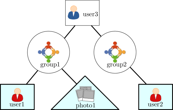
Figure 1. Example query on a photo-sharing network: find the most important nodes of types (user3, group1, group2) for a given triple of specified nodes of types (photo1, user1, user2).

These types of rich query semantics also appears in other contexts, e.g., root-cause analysis in distributed systems. The Vitrage service for OpenStack (Vit, 2018) makes use of path and tree patterns to specify rules for automatic root cause deduction of alarms raised by virtual machines and hardware. Large OpenStack deployments—involving thousands of hosts and tens of thousands of virtual machines and hardware components—necessitate pattern matching algorithms to deduce the root cause of such patterns in near real-time.

We focus on efficient solutions for acyclic pattern queries on general labeled graphs. To this end, we propose the notion of any-$k$ algorithms, a novel variant of top-$k$ algorithms. A top-$k$ algorithm exploits knowledge about the given $k$ to produce the top-$k$ lightest patterns faster than the “full enumeration” algorithm (which first produces all results and then ranks them by weight). In practice, it is difficult for users to know the value of $k$ upfront (“when will I have seen enough?”). An any-$k$ algorithm addresses this issue by not requiring a pre-set value for $k$. Instead, an any-$k$ algorithm

1. returns the top-ranked result as quickly as possible,

2. then returns the second-ranked result next, followed by the third-ranked, and so on,

3. until the user is satisfied and terminates the process.

In other words, the ranked enumeration can be stopped anytime and should then return as many top results as possible.

The queries we are interested in correspond to subgraph isomorphism, which is known to be hard in general. In particular, subgraph isomorphism on homogeneous graphs is already NP-complete in the size of the query (even for the path case as Hamiltonian path is a special case). And labeled graphs contain unlabeled graphs as a special case. On the other hand, labels provide more opportunities for achieving better performance in practice by exploiting heterogeneity where present. Note that a key reason for hardness of isomorphism lies in the “non-repetition constraint,” i.e., the same graph node cannot occur more than once in an answer. Without this constraint, pattern search would correspond to the easier subgraph homomorphism problem which can be solved in PTIME.

Our approach is based on three key insights: (1) Constraints on node or edge labels can dramatically reduce the number of matching results; (2) Mutually exclusive type labels “narrow the gap” in cardinality between the set of isomorphic subgraphs and the set of homomorphic subgraphs (which includes all isomorphic ones). The reason is that query pattern nodes of different types cannot be mapped to the same graph node, even when the algorithm is only searching for homomorphism. In the example photo-sharing network, users and photos cannot stand in for a group node. In the extreme, if all nodes in the query pattern have different types, then any solution for subgraph homomorphism also satisfies isomorphism. This suggests an approach that aggressively prunes for the homomorphism case and then filters based on node repetitions in the result patterns; and (3) In many real-world cases, output size is small relative to the combinatorial size of the pattern search space. Hence algorithm complexity bounds based on output size promise to deliver practically meaningful performance guarantees.

Overview of the Solution. Our approach combines three conceptually separate steps into a two-phase algorithm.

1) The search space of possible homomorphic patterns is pruned to the provably smallest representation of the original graph. We use insights from the well-known Yannakakis algorithm (Yannakakis, 1981) for evaluating answers to acyclic conjunctive queries to create this representation in just one bottom-up and a subsequent top-down sweep through the query tree.

2) We devise a novel any-$k$ algorithm for enumerating homomorphic tree patterns. It uses dynamic programming to perform a bottom-up cost calculation, followed by a top-down guided search.

3) A final pruning step removes those homomorphic patterns that do not satisfy the isomorphism requirement.

We show how to combine the first two steps into just one bottom-up and one top-down phase. We then integrate the third step into the combined top-down phase. Our experiments show that even on graphs with millions of nodes and tens of millions of edges, we can return the top-ranked results in just a few milliseconds, whereas alternative approaches would take orders of magnitude longer. Our implementation can be downloaded from (Cod, 2018).

Main contributions. We devise KARPET (Kernelization And Rapid Pruning-based Exploration for Tree patterns), a novel and highly performant any-$k$ algorithm that can quickly identify top-ranked tree patterns in large graphs, then return the next lower-ranked ones when given extra time.

1) KARPET is designed as an anytime ranking algorithm that enumerates homomorphic subtrees in order of total edge weight with strong theoretic guarantees: We show that our worst-case time complexity for returning all homomorphism results is identical to full enumeration. In addition, KARPET provides strong upper bound guarantees for the time to return the top-ranked homomorphism result, as well as the time between returning a homomorphism result and the next. For cases with “small gap” between homomorphism and isomorphism, i.e., when “sufficiently many” homomorphic patterns are also isomorphic patterns, these guarantees carry over to subgraph isomorphism.

2) We propose fast and effective local pruning operations that exploit the heterogeneity of labeled graphs, proving that they also guarantee strong global pruning properties. Intuitively, for subgraph homomorphism, we show that inexpensive pruning based on 1-node neighborhoods efficiently removes all candidate nodes that are not part of any result pattern.

3) In contrast to a lot of theoretical work on subgraph isomorphism algorithms, our algorithm is output-sensitive—its worst case complexity depends on the output size, which is smaller when the graph and the query are more heterogeneous, rather than being exponential in the size of the query pattern.

4) We show how to speed up the search for top-ranked isomorphic answers by pushing the pruning for non-repeating nodes into the incremental result enumeration algorithm.

2. Problem Definition and Hardness

Our goal is to find the lightest subgraphs of a labeled graph $G$ that are isomorphic to a given tree pattern $Q$. Instead of returning all results at once after a long wait time, we set out to devise an anytime algorithm, which returns the top-ranked match as quickly as possible and then incrementally returns the remaining results over time.

Definition 2.1 (Any-$k$ algorithm).

An any-$k$ algorithm is a variant of a top-$k$ algorithm in which $k$ is not known at the start of the algorithm. The algorithm can be interrupted anytime, returning the top-$k$ results with $k$ being as large as possible.

We define the weight of a pattern as the sum of edge weights. This also supports search for the “most reliable” pattern based on probabilities assigned to edges. Finding the pattern with the greatest probability of being connected, assuming independence, is equivalent to maximizing the sum of the logarithms of the edge probabilities. For our problem with a fixed query pattern, lightest and heaviest pattern search can be easily converted into each other. It is also straightforward to modify our approach to support pattern weight defined as minimum or maximum of edge weights. We present the formal definitions next. Table 1 summarizes important notation.

Table 1. Notation used in this paper

Symbol	Definition
$G(V,E)$	A labeled graph with node set $V$ and edge set $E$
$L$	Set of node labels
$\varphi()$	Function mapping nodes to labels
$w()$	Function mapping edges to weights
$Q(V_{Q},E_{Q})$	Tree pattern with node set $V_{Q}$ and edge set $E_{Q}$
$\psi()$	Required labels for a graph node matched to a query node
$\bot(Q)$	Set of leaf nodes (or terminals) in $Q$
$\top(Q)$	Chosen root node in $Q$
$N(v,\ell)$	Set of neighbors of $v$ in $G$ with label $\ell$
$\lambda()$	Function mapping query nodes $V_{Q}$ to graph nodes $V$

Definition 2.2 (HIN, labeled graph).

A Weighted Heterogeneous Information Network (HIN) is a labeled undirected graph $G=(V,E,\varphi,w)$, where $V$ is a set of vertices, $E$ is a set of edges, $\varphi$ is a node labeling function $\varphi:V\rightarrow L$, and $w$ is an edge weight function $w:E\rightarrow\mathbb{R}$.

In many HINs, a node has at least two different kinds of labels: a unique node ID and a type (or class). In the photo-sharing network example (see Example 1.1), the labeling function assigns types such as “user” or “photo” to each node. Our approach can be easily extended to include multiple labels per node, as well as (multiple) edge labels, node weights, and directed edges. We omit these straightforward generalizations in order to simplify the exposition.

Given a vertex $v\in V$ and label $\ell\in L$, we use $N(v,\ell)$ to denote the set of all neighbors of $v$ with label $\ell$, i.e., $N(v,\ell)\coloneqq\{u:(v,u)\in E\land\varphi(u)=\ell\}$.

Definition 2.3 (Tree pattern or query $Q$).

Given a labeled graph $G=(V,E,\varphi,w)$, a tree pattern is a rooted tree $Q=(V_{Q},E_{Q},\psi)$ in which each node $v\in V_{Q}$ has a label constraint $\psi:V_{Q}\rightarrow L$. We use $\top(Q)\in V_{Q}$ to denote the root of the tree and $\bot(Q)$ to denote the set of its leaves (or terminals, i.e. nodes of degree one).

The labeling constraint can encode the selection of specific nodes or node types. For example, in the photo-sharing network scenario, setting $\psi$ for user1 to be the ID of a specific user node limits the candidate set for user1 to just this one graph node. Similarly, setting $\psi$ to the label encoding the type “group” will enforce that only graph nodes representing groups, but not users or photos, will be considered.

Notice that $Q$ being rooted is not a restriction: any node in a tree can be chosen to be the root. We merely make use of the fact that the tree pattern is rooted in order to more easily describe our algorithms.

Definition 2.4 (homomorphic match or result pattern).

A homomorphic result pattern (or homomorphic match) of query $Q$ is a graph $(V^{\prime}\subseteq V,E^{\prime}\subseteq E)$ such that there exists a function $\lambda:V_{Q}\rightarrow V^{\prime}$ with the following properties: (1) $\forall u\in V_{Q}:\psi(u)=\varphi(\lambda(u))$, and (2) $\forall(u,v)\in E_{Q}:(\lambda(u),\lambda(v))\in E^{\prime}$. The weight of a result pattern is defined as $\sum_{(u,v)\in E^{\prime}}w(u,v)$.

Definition 2.5 (match or result pattern).

An (isomorphic) result pattern (or match) of query $Q$ is a homomorphic result pattern $(V^{\prime}\subseteq V,E^{\prime}\subseteq E)$ with a bijective mapping function $\lambda:V_{Q}\xrightarrow[]{\text{1:1}}V^{\prime}$.

The above definitions make it clear that the set of isomorphic matches is a subset of the homomorphic matches; and can be obtained by removing all those homomorphic matches where multiple query nodes are mapped to the same graph node.

In the discussion below we will also refer to partial patterns (or partial matches) for intermediate results of the computation. These are incomplete instances where some of the query nodes are mapped to NIL by $\lambda$. The direct successor of a partial match is one where exactly one of the NIL targets is replaced by a graph node, growing the pattern by one additional node. With successor we refer to any partial or complete match in the transitive closure of direct successor.

For fast access to $N(v,\ell)$, we rely on GraphEdge, a two-level hash index constructed offline for $G$. It maps a given node ID $v$ to another hash table, which in turn maps a given label $\ell$ to the set $N(v,\ell)$ of neighbors of $v$ with label $\ell$. If no label is specified, all nodes and corresponding edge weights in the secondary hash table for $v$ are returned. This index can be bulk-created from scratch in time linear in the graph size, and updated in time linear in the size of the changes.

Hardness. In general, even the decision version of sub-graph isomorphism, i.e., to determine if a given query graph is isomorphic to a sub-graph of $G$, is NP-complete. When the sub-graph is connected acyclic (i.e., a tree), the best worst-case time bound for the decision problem is a parameterized algorithm of Koutis and Williams (Koutis and Williams, 2016) that requires $O(2^{|V_{Q}|}\texttt{poly}(|V|))$ time. Their algorithm also has matching conditional lower bounds (Krauthgamer and Trabelsi, 2017): achieving a bound of $O(2^{(1-\varepsilon)|V_{Q}|}\texttt{poly}(|V|))$ time, for any constant $\varepsilon>0$, would falsify a longstanding conjecture. Note that, since the decision problem is hard, the any-$k$ problem discussed here is at least as hard.

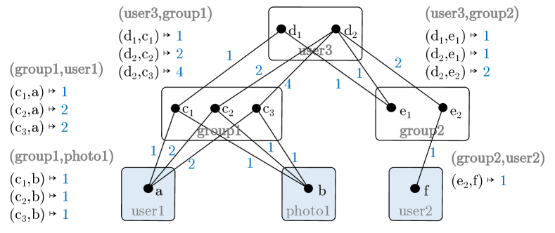
Figure 2. Candidate instances for matching the example query in Figure 1. Edge sets are named based on the corresponding pairs of adjacent nodes in the query pattern.

In practice we often know specific node instances such as $a$ for user1 in the photo-sharing network example, and can dramatically reduce the pattern search space by exploring $G$ starting from these nodes. Still, as Figure 2 illustrates, one cannot tell from the immediate neighborhood of node $a$, if edge $(a,c_{1})$ will belong to top-ranked results, or any results at all. Worse yet, not even the 3-hop neighborhood of $a$ will answer this question. Hence a pattern search algorithm might suffer from expensive backtracking or the inability to determine, without extensive graph traversal, when the top-$k$ lowest-weight patterns have been found.

To the best of our knowledge, KARPET is the first algorithm for ranked retrieval of graph query patterns that performs pruning and exploration based on “local” information, while provably guaranteeing to make the right decisions “globally.”

3. Any-k Algorithm

We next present an approach for sub-graph homomorphism; this is a relaxation of sub-graph isomorphism in that we do not require the mapping $\lambda$ from query nodes to tree-pattern nodes to be bijective (in other words, a node can be repeated in the result pattern). Section 5 extends the approach for isomorphism.

KARPET consists of two phases: 1) a bottom-up sweep from leaves to the root of $Q$, and 2) a top-down depth-first traversal from root to leaves. The first phase prunes some of the spurious candidates and creates a “candidate graph” (discussed below) with “minimum subtree weights.” The second phase prunes the remaining spurious candidates and performs a search guided by the subtree weights. Here the term spurious candidate refers to a node or edge of the input graph that does not appear in any of the query results.

3.1. Bottom-Up Phase

Algorithm 1 Bottom-up Subtree Weight Computation

Input: query $Q$, node neighborhood index $N(v,\ell)$

Output: $\texttt{CandNode}:u\mapsto[c\mapsto[u^{\prime}\mapsto w_{\min}]]$

Output: $\texttt{CandEdge}:(u,u^{\prime})\mapsto[c\mapsto c^{\prime}]$

1: // For each leaf node in the query tree, find graph nodes with required label, add them to the candidates, and set their weights to 0

2:for $u\in\bot(Q)$ do

3:    $\forall c\in V.\varphi(c)=\psi(u):\texttt{CandNode}(u).\textsc{Insert}(c\mapsto(\textrm{NIL}\mapsto 0))$

4: // Traverse remaining query nodes in any bottom-up order

5:for $u\in\textsc{Traversal}(V_{Q})$ do

6:     //($i$) Find candidate edges adjacent to candidates in all children $u^{\prime}$

7:    for children $u^{\prime}$ of $u$ in $Q$, and candidates $c^{\prime}\in\texttt{CandNode}(u^{\prime})$ do

8:         for neighbors $c\in N(c^{\prime},\psi(u))$ do

9:             $\texttt{CandEdge}(u,u^{\prime}).\textsc{Insert}(c\mapsto c^{\prime})$              

10:     //(ii) Keep only candidates with edges to each of the children of $u$

11:    $C=\bigcap_{u^{\prime}\textrm{ child nodes of }u}\texttt{CandEdge}(u,u^{\prime}).\textsc{Keys}$

12:     //(iii) Find min subtree weights for reachable candidates to children

13:    for $c\in C$ and all children $u_{i}$ of $u$ do

14:         $C^{\prime}=\texttt{CandEdge}(u,u^{\prime}).\texttt{Get}(c)$

15:         $w_{i}\leftarrow\min_{c^{\prime}\in C^{\prime}}[w(c,c^{\prime})+\textsc{Weight}(c^{\prime})]$

16:         $\texttt{CandNode}(u).\textsc{Insert}(c\mapsto(u_{i}\mapsto w_{i}))$     

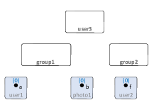
(a)

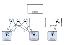
(b)

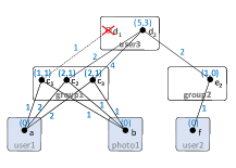
(c)

Figure 3. Minimal subtree weight computations: (a) after traversing all leaves, (b) after traversing middle level, (c) after finishing at the root. Numbers above node candidates indicate minimum sub-tree weights stored in CandNode; numbers on edges indicate edge weights stored in CandEdge.

The bottom-up phase traverses the query tree in any bottom-up order and constructs a “candidate graph” consisting of two index structures: (1) $\texttt{CandNode}(u)$ returns for query node $u$ a hash index that maps a node candidate $c$ to a list of minimum subtree weights, with one weight for each of $c$’s children. (2) $\texttt{CandEdge}(u,u^{\prime})$ returns for each query edge between a node $u$ and its child $u^{\prime}$ a hash index that maps a candidate node $c$ of $u$ to all adjacent candidates $c^{\prime}$ of $u^{\prime}$.

We illustrate Algorithm 1 with Figures 3(a), 3(b), and 3(c). It first inserts candidate nodes for each query leaf node $u$ into the corresponding candidates $\texttt{CandNode}(u)$, setting their weights to zero (line 2). Note that leaves do not have children, hence the NIL value in the expression. In Figure 3(a) there is a single candidate per leaf, but in practice it can be a larger subset of $V$ for each query leaf, depending on the node constraints. Then, for each query node $u$, the algorithm ($i$) finds possible candidate nodes, ($ii$) prunes them, and ($iii$) calculates the minimum subtree weights

In more detail: ($i$) for each query edge leading to a child $(u,u^{\prime})$, it first finds all candidate edges $(c,c^{\prime})$, storing the map $\texttt{CandEdge}:(u,u^{\prime})\mapsto[c\mapsto c^{\prime}]$ (line 8). ($ii$) Then, the algorithm only keeps the list of candidates for each query node that are reachable from candidate instances in all leaves of the query node (line 11): In Figure 3(c), the list of candidates for query node group1 is $\{c_{1},c_{2},c_{3}\}$. Notice how spurious candidates not reachable from the leaves, e.g., $e_{1}$ in group2, are not even accessed (compare with Figure 2). Similarly, while $d_{1}$ in user3 is reachable from the left, it is not reachable from the right subtree and is thus automatically pruned as well. ($iii$) Then, the algorithm finds for each reachable node, the min weight along each query edge $(u,u^{\prime})$ starting at $c$ (line 16). For example, in Figure 3(c), the left weight $5$ for $c_{2}$ is computed as the minimum of weights for following $(d_{2},c_{2})$, which is 5 as the sum of the weight of edge $(d_{2},c_{2})$ (= 2) plus the weight of $c_{2}$ (= 2+1), or for following $(d_{2},c_{3})$, which is 7 as the sum of the weight of edge $(d_{2},c_{2})$ (= 4) plus the weight of $c_{3}$ (= 2+1). Notice we use here $\textsc{Weight}(c)$ as short form for the sum of weights at a node $c$, which we get from CandNode. The two new created indices speed up finding adjacent edges in a subtree of the query pattern during top-down traversal.

3.2. Top-Down Phase

The second part of our algorithm performs top-down search, starting at the root node and proceeding downward to the leaves. This is essential for two reasons: First, the pre-computed subtree weights provide information to guide the search to the lightest patterns before exploring the heavier ones. Second, the top-down traversal implicitly prunes all remaining spurious candidates for sub-graph homomorphism, as we will prove in Section 4. Again, pruning actually happens implicitly by not reaching those candidates. To see the latter, consider group1 candidate $c_{1}$ in Figure 3(c). It is spurious, but could not be removed by the bottom-up sweep. However, it will never be accessed during top-down traversal, because $d_{1}$ was never recorded in CandNode by Algorithm 1.

Algorithm 2 Prioritized Search (front-element optimization not shown)

Input: Tree pattern $Q$, CandNode, CandEdge

Output: All matches of $Q$, one-by-one in increasing order of weight

1: //Initialize pq with all candidates of the query root node

2:$\texttt{pq}\leftarrow\textsc{PriorityQueue}()$

3:for $c\in\texttt{CandNode}(\top(Q))$ do

4:    $Z\leftarrow$ partial tree $(c)$ consisting of just one node

5:    $\texttt{pq}.\textsc{Insert}(\textsc{Weight}(c),Z)$

6: //Expand pq until all results returned

7:while pq.Size ¿ 0 do

8:     $(\texttt{oldkey},Z)\leftarrow\texttt{pq}.\textsc{Pop-Minimum}$

9:    if $Z$ is a complete match then

10:         return $Z$

11:    else

12:         $(u,u^{\prime})\leftarrow\textsc{NextPreorder}(Q,Z)$ $\triangleright$ Edge to expand pattern

13:         for $c\in\texttt{CandNode}(u)$ do

14:             for $c^{\prime}$ returned by $\texttt{CandEdge}(u,u^{\prime}).\textsc{Get}(c)$ do

15:                 $Z^{\prime}=Z.\textsc{Append}(c^{\prime})$

16:                 $\texttt{newkey}\leftarrow\texttt{oldkey}-\texttt{CandNode}(u).\texttt{Get}(c,u^{\prime})+\phantom{a}\phantom{a}\phantom{a}\phantom{a}\phantom{a}\phantom{a}\phantom{a}\hskip 59.75078pt\phantom{a}w(c,c^{\prime})+\textsc{Weight}(c^{\prime})$

17:                 pq.Push($\texttt{newkey},Z^{\prime})$                           

Algorithm 2 shows the pseudo-code for top-down guided search. Initially, all candidates $c$ in the query root $r$ are inserted into priority queue pq (line 3), with their priorities set to the sum of the candidate’s weights. In Figure 3(c), there is a single candidate, $d_{2}$, of weight $5+3=8$. Then the algorithm repeatedly pops the top element from pq and expands the partial pattern using pre-order traversal. Function NextPreorder returns the edge, as the pair of parent and child node, along which the partial pattern will be expanded next (line 12). The priority value of each expanded partial match is defined as the sum of the pattern’s edge weights plus the sum of the weights of the unexplored subtrees. In the example, partial match $(d_{2},c_{2})$ is inserted into pq with priority 8 = 2 (edge weight) + (2+1) (weights of $c_{2}$) + 3 (weight of right subtree of $d_{2}$). Similarly, partial match $(d_{2},c_{3})$ is inserted with priority 4+(2+1)+3 = 10. Note that those values are computed incrementally during traversal (line 16). Consider expansion of $(d_{2})$ to $(d_{2},c_{3})$. Priority of $d_{2}$ was 8, with weight 5 for the newly expanded subtree rooted at group1. After retrieving $c_{3}$ from CandEdge, priority of $(d_{2},c_{3})$ is computed as 8 (old) - 5 (newly expanded subtree) + 4 (weight of edge $(d_{2},c_{3})$ ) + 3 (priority of $c_{3}$) = 10 (line 16 in Alg. 2). Then $(d_{2},c_{2})$ is popped next, and expanded to partial match $(d_{2},c_{2},a)$ with priority 8 = 8 - 2 + 2 + (0+0). This pattern is then expanded next to $(d_{2},c_{2},a,b)$, $(d_{2},c_{2},a,b,e_{2})$, and finally $(d_{2},c_{2},a,b,e_{2},f)$—all with the same priority of 8. The latter is output as the minimal-weight solution. Only then will partial match $(d_{2},c_{3})$ with the higher priority value 10 be expanded analogously. Each expansion operation requires a pop operation from priority queue, visiting potential edges once.

4. Algorithm Analysis

All results in this section are for the relaxed version of the problem, based on sub-graph homomorphism instead of isomorphism. We discuss in Section 5 how to extend them to the isomorphism case. Proofs were omitted due to space constraints, but can be found in the extended version (Yang et al., 2018).

4.1. Minimality of Candidate Graph

We show that during top-down search (Alg. 2), no spurious candidate node will ever be accessed. A candidate node $c$ for a query node $q$ is “spurious” if there does not exist any homomorphic result pattern where $c$ is matched to $q$. Ensuring that no spurious nodes are accessed is crucial for proving strong upper bounds on the algorithm cost.

Theorem 4.1.

If node candidate $c\in\texttt{CandNode}(q)$ for query node $q\in V_{Q}$ is accessed by Alg. 2, then there exists a homomorphic result pattern where $\lambda(q)=c$.

4.2. Each Pop, One Result—In Order

Next, we show a powerful result that is crucial in establishing important algorithm properties: During the top-down guided search, for each query result there is at most one push and at most one pop operation on priority queue pq. For this, we need the following lemmas.

Lemma 4.2.

The priority value of a partial pattern $P$ is always less than or equal to the priority of all its successors.

Lemma 4.3.

Assume that Alg. 2 popped partial pattern $P=(c_{1},c_{2},\ldots,c_{j})$, $j<|V_{Q}|$, of priority $w$ from pq. Then there exists a direct successor $(c_{1},c_{2},\ldots,c_{j},c_{j+1})$ that has the same priority $w$.

Lemmas 4.2 and 4.3 immediately imply:

Corollary 4.4.

If the last pop operation on pq returned an incomplete pattern $P$, then one of the direct successors of $P$ will have priority equal to the minimum priority over all elements in pq.

Example 4.5.

Consider the changes of pq for the example in Figure 3(c). Initially it contains $[(d_{2}):8]$, the sole root node candidate with priority 5+3=8. This element is popped and expanded along edges $(d_{2},c_{2})$ and $(d_{2},c_{3})$. The priority of the former is 2 (weight of edge $(d_{2},c_{2})$) plus (2+1) (subtree weights of $c_{2}$) plus 3 (right subtree weight of $d_{2}$) = 8. It is identical to the initial priority of $d_{2}$, because edge $(d_{2},c_{2})$ is the one that determined the minimum left subtree weight of 5 in $d_{2}$. For $(d_{2},c_{3})$, priority is 10 due to the higher weight of edge $(d_{2},c_{3})$. After these two patterns are pushed, pq contains $[(d_{2},c_{2}):8,(d_{2},c_{3}):10]$. The next pop delivers $(d_{2},c_{2}):8$, which is expanded to $(d_{2},c_{2},a):8$, followed by repeated pop and push operations on this pattern, every time obtaining the same priority of 8, until the top result $(d_{2},c_{2},a,b,e_{2},f)$ of weight 8 is completed. Only then will expansion of $(d_{2},c_{3}):10$ commence.

Front-element optimization. Based on Corollary 4.4, we next introduce an important optimization to Alg. 2. Since the corollary guarantees that one of the direct successors of the partial pattern popped before will have a minimal priority value, we avoid the push-pop cycle for it and keep expanding it directly, only pushing the other direct successors. More precisely, assume the algorithm just popped partial match $P=(c_{1},c_{2},\ldots,c_{i})$ of priority $w$ from pq. While expanding this pattern by one more node, it keeps in memory the first direct successor $P^{\prime}=(c_{1},c_{2},\ldots,c_{i},c^{\prime}_{i+1})$ encountered that also has priority value $w$, pushing all other direct successors to pq. This way the algorithm still works on a min-priority element, but avoids the push-pop cycle for it. This seemingly minor optimization has strong implications as formalized in the following theorems.

Theorem 4.6.

Using front-element optimization, for any $k$, the $k$-th pop operation from pq produces the $k$-th lightest homomorphic result pattern, possibly requiring additional push operations, but no more pop operations until this result pattern is returned.

Corollary 4.7.

No matter how many results are retrieved, Alg. 2 never performs more than $r_{H}$ push operations on pq in total. Here $r_{H}$ denotes the number of homomorphic subtrees in $G$.

This follows directly from Theorem 4.6 and the following observation. Assume the algorithm continues to run until all query results are found. At that point it has removed all partial matches from pq and the queue is empty. Theorem 4.6 implies that retrieving all results requires exactly $r_{H}$ pop operations. If the total number of push operations exceeded this, then the queue would not be empty. (And obviously, any execution of Alg. 2 that stops before returning all results will only have performed a subset of the push operations executed by the time all results are returned.)

4.3. Algorithm Cost

To avoid notational clutter, we treat the size of the query pattern as a small constant and omit it from most formulas. (Note that pattern size is equal to the number of edges in $E_{Q}$, e.g., 5 in the photo-sharing network example.) It is straightforward to extend the formulas by including $|E_{Q}|$ as a variable.

Algorithm 1. Theoretical worst case cost is $\mathrm{O}(|E|)$, i.e., linear in graph size: for each of the query pattern edges, in the worst case all graph edges are accessed. The time for constructing CandEdge and CandNode adds a constant overhead per edge processed. In practice, only a small fraction of $E$ will be accessed because of the label constraints. In particular, by using GraphEdge in line 8 in Alg. 1, all neighbors of matching types (labels) are accessed in time linear in the number of these neighbors. Space cost is upper bounded by the combined size of CandNode and CandEdge, i.e., cannot exceed $|E_{Q}|$ times input graph size.

Algorithm 2. The results from Section 4.2 lead to strong guarantees. Space complexity of Alg. 2 is equal to the maximum size of the priority queue. Corollary 4.7 immediately implies:

Theorem 4.8.

Space cost of Alg. 2 is upper bounded by $r_{H}$, the total result size for sub-graph homomorphism.

From a user’s point of view, the time it takes to produce the next lower-ranked result is crucial:

Theorem 4.9.

The initial latency for Alg. 2 to return the top-ranked homomorphic match, and also the time between returning any two consecutive homomorphic matches, is $\mathrm{O}(\mathrm{outDegree}+\log r_{H})$. Here $\mathrm{outDegree}\leq r_{H}$ is greater of (1) the number of candidates in the root node and (2) the maximum cardinality of the set of adjacent node candidates $c^{\prime}$ in $\texttt{CandEdge}:(u,u^{\prime})\mapsto[c\mapsto\{(c^{\prime},w(c,c^{\prime}))\}]$ for any query graph edge $(u,u^{\prime})$ and candidate $c$.

These strong results show that KARPET can effectively exploit selective label constraints. For instance, if there are a thousand homomorphic subgraphs in $G$, then Theorems 4.8 and 4.9 guarantee that Alg. 2 will never store more than a thousand partial matches in memory and will perform at most a thousand (inexpensive) computation steps to deliver the next result to the user—no matter how big or connected the given graph!

We show next that the anytime property of KARPET, i.e., that it can deliver the top-ranked results quickly and then the next ones on request, incurs no performance penalty for producing all homomorphic matches:

Theorem 4.10.

The lower bound for producing all homomorphic result patterns is $\Omega(r_{H})$; sorting them costs $\mathrm{O}(r_{H}\log r_{H})$. Alg. 2 has matching total time complexity $\mathrm{O}(r_{H}\log r_{H})$.

5. Homomorphism to Isomorphism

KARPET as introduced in Section 3 returns homomorphic matches. To obtain the desired isomorphic matches, function $\lambda$ mapping query nodes to tree-pattern nodes has to be bijective. To guarantee this, one simply has to filter out all results where different query nodes are mapped to the same graph node. Instead of filtering on the final result, KARPET can perform early pruning by checking in line 15 in Alg. 2 if newly added node $c^{\prime}$ already appears in partial match $Z$—discarding $Z^{\prime}$ if it does. This modification has the following implications for the cost analysis results in Section 4.3.

Since some of the items previously pushed to priority queue pq will now be discarded early, space consumption as well as computation cost of KARPET are lower than for finding all subgraph homomorphism results. However, worst-case complexity as established by Theorems 4.8 and 4.10 remains the same. And the guarantees for the time between results (Theorem 4.9) is weaker: In the worst case, e.g., when only the very first and the very last of the homomorphic matches represent isomorphic results, then time between consecutive results grows from $\mathrm{O}(\mathrm{outDegree}+\log r_{H})$ to $\mathrm{O}(r_{H}\log r_{H})$. Fortunately, as our experiments indicate, heterogeneity indeed results in a small gap between homomorphism and isomorphism, i.e., real-world performance is closer to $\mathrm{O}(\mathrm{outDegree}+\log r_{H})$.

6. Experiments

Our experiments evaluate running time, memory consumption, and size of the search space explored by $KARPET$ on several query templates and four data sets against two baseline algorithms. In order to allow reproducible results, our code can be downloaded from our project page (Cod, 2018).

Baseline algorithms. We chose two baselines that allow us to evaluate the relative contribution of our two key steps (pruning the search space, and guided search) to the performance of $KARPET$.

Unguided first calculates all results from the candidate graph and only then ranks them. Since it uses our pruned search space, but does not include any prioritizing of query results, it serves as a baseline to evaluate the contribution of our guided search phase.

Backbone is intended to evaluate the effect of our aggressive tree-based pruning strategy. It extends the state-of-art top-$k$ algorithm for path queries on HINs (Liang et al., 2016). First, it identifies the longest terminal-to-terminal path $R$ in the tree pattern $Q$ (called the “backbone” of $Q$). It then incrementally retrieves the lightest backbone instances in $G$ one-by-one. Note that such an instance is a partial match with smaller unmapped subtrees “hanging off” the backbone path. Thus, we can execute Unguided on each such subpattern, yielding a divide and conquer algorithm. Since each subpattern is independent, we extract the lightest instance of each subpattern, and merge these solutions with the backbone instance. This involves checking for repeat node occurrences to enforce isomorphism. Then the next heavier subtree matches are explored etc. Given a pre-defined value of $k$, the algorithm can prune the set of remaining backbone instances every time a new full match is found. In all our experiments, we supply the ultimate value of $k$ to Backbone, to explore the best possible performance this algorithm might achieve (if it was able to guess the correct value of $k$ from the start).

Datasets. We use four well-known heterogeneous datasets: Flickr (Fli, 2018), DBLP (Liang et al., 2016), Enron (Liang et al., 2016), and Yelp (Yel, 2017). Figure 4 gives an overview of their properties. Notice that Enron, DBLP and Flickr have denser graphs than Yelp. In order to create weights for individual edges, we used the age of the edge with an exponential decay based on the difference between edge creation time and query time.

Dataset	$|V|$	$|E|$	$|L|$
Flickr	2,007,369	18,147,504	3
DBLP	2,241,258	14,747,328	4
Enron	46,463	613,838	4
Yelp	4,301,900	7,059,472	6

Figure 4. Dataset statistics

Query templates. We created five different pattern templates listed in Fig. 5. For each pattern, we chose 300 different assignments of actual nodes to the query leaves, which gave us 300 queries per template, for a total of 6,000 query instances across all datasets.

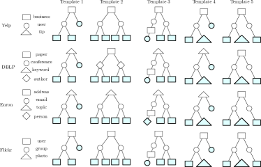
Figure 5. Templates used to generate queries for each dataset. Shapes indicate node types; the cyan-colored nodes are terminals.

Performance metrics. We vary $k$ between 1 and total number of results, and compare the algorithms on three performance metrics. 1) Running time: We measure the time between having loaded the dataset into memory and returning the k-th result, reporting the average for each template. 2) Memory consumption: We report the maximum number of nodes (i.e., partial matches weighted by the number of matched nodes they contain) stored at any time during the execution of each algorithm. 3) Size of search space: We report the total number of partial matches (weighted by the number of matched nodes they contain) that are stored during execution.

Experimental setup. Experiments were run on an Intel Xeon CPU E5-2440 1.90GHz with 200GB of memory running Linux. We compiled the source code with g++ 4.8 (optimization flag O2).

6.1. Discussion and Highlights

To justify our “solving isomorphism through homomorphism” approach, we also ran KARPET with node-repetition check turned off. This produces all homomorphic matches, from which we can then determine offline how many were also results for the isomorphism case. We plot both numbers as we increase $k$ in Figure 6. It shows a representative result, obtained from the Enron dataset using a query from Template 1. The small gap between the lines confirms that the vast majority of homomorphic matches are also isomorphic result patterns.

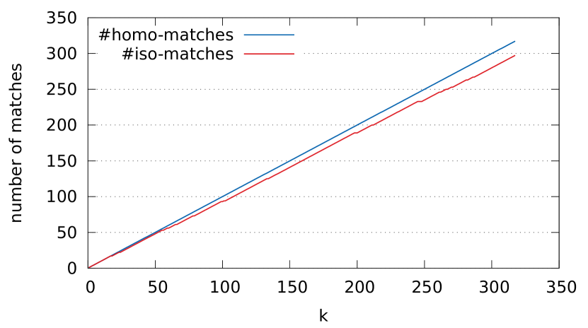
Figure 6. Number of isomorphic and homomorphic matches for an instance of Template 1 on the Enron dataset.

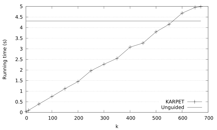
Figure 7. Running time for increasing k until all results are returned, for KARPET and Unguided.

Figure 7 shows a representative result comparing KARPET to Unguided, which bulk-computes the entire output and hence is not affected by the choice of $k$. It is clearly visible how our any-$k$ algorithm continuously returns the top-ranked results in order, with very low latency between consecutive outputs. By the time Unguided finally returns the first match, KARPET has already delivered more than 85% of all matches. In the end, it took KARPET 4.98s to output all matches. For comparison, bulk-computation by Unguided took 4.31s, indicating a small overhead of 0.67s for supporting the anytime property.

Data	Algorithm	T1	T2	T3	T4	T5
Flickr	KARPET	43.86	58.17	99.28	20.12	81.92
	Unguided	2200	2085	5951	2021	5518
	Backbone	2946	9678	3033	4114	9963
DBLP	KARPET	9.51	8.87	104.33	8.67	8.15
	Unguided	1090	1936	1995	814	1110
	Backbone	839	502	337	1109	1059
Enron	KARPET	10	57	29	57	104
	Unguided	202	1036	1013	669	891
	Backbone	4914	18925	5124	7056	11075
Yelp	KARPET	0.11	0.13	0.78	0.20	0.15
	Unguided	1.68	1.79	2.27	1.40	2.06
	Backbone	3.84	3.53	1.02	3.82	3.02

Table 2. Average running time (milliseconds) for each dataset, algorithm, and template. Cells with the least running time in the three algorithms are marked gray.

Data	Algorithm	T1	T2	T3	T4	T5
Flickr	KARPET	278	286	1212	458	1957
	Unguided	1212	294	17560	833	61603
	Backbone	460	139	76	939	1057
DBLP	KARPET	162	146	387	251	253
	Unguided	162	146	409	251	253
	Backbone	29	35	26	72	103
Enron	KARPET	459	676	546	727	713
	Unguided	477	697	569	745	728
	Backbone	188	109	11	168	87
Yelp	KARPET	1.02	1.02	1.36	1.01	1.02
	Unguided	1.02	1.02	1.36	1.01	1.02
	Backbone	1.03	1.02	1.00	1.01	1.02

Table 3. Average memory measured by the max number of nodes stored, for each dataset, algorithm, and template. Cells using the least memory are marked gray.

Data	Algorithm	T1	T2	T3	T4	T5
Flickr	KARPET	1.16-e6	1.18-e6	9.29-e5	1.12-e4	1.56-e6
	Unguided	5.41-e6	1.55-e6	1.96-e7	1.52-e5	2.20-e7
	Backbone	5.37-e6	1.99-e6	1.16-e6	1.02-e7	8.04-e6
DBLP	KARPET	4.84-e4	3.98-e4	5.48-e4	9.35-e4	4.55-e4
	Unguided	7.25-e5	3.35-e5	1.58-e6	2.16-e5	8.91-e5
	Backbone	4.64-e5	1.68-e5	2.91-e5	9.38-e5	9.57-e5
Enron	KARPET	4.22-e4	1.13-e5	7.39-e4	1.29-e4	3.52-e4
	Unguided	8.41-e5	9.50-e5	9.11-e5	8.93-e5	8.60-e5
	Backbone	1.31-e6	8.86-e5	1.39-e6	3.07-e5	5.74-e5
Yelp	KARPET	58	99	191	51	104
	Unguided	58	99	233	51	104
	Backbone	45	100	17	48	62

Table 4. Average search space measured by weighted total number of partial matches, for each dataset, algorithm, and template. Cells exploring the least search space are marked gray.

For each template (fixing $k=5$) we show the average running time, memory usage, and search space of our algorithm, along with the two baselines, on all four datasets in Tables 2, 3, and 4. In terms of average running time, KARPET outperforms the baselines in all cases. On DBLP, we can see 100x faster running time compared to Unguided, and 10x speedup compared to Backbone. We make the following detailed observations about these results.

6.1.1. Varying the Dataset

We observed that KARPET’s margin of improvement over the baselines is generally greater on denser graphs. Higher density leads to more matches, which KARPET can handle best, because it prioritizes the search based on subtree weight more effectively than the two baselines. The Yelp graph is extremely sparse, causing many queries to have only one or two matches. For those queries, all three algorithms behave nearly identically, e.g., running time for a typical single-match query on Yelp was $0.15$ msec for KARPET, $0.2$ msec for Unguided, and $0.16$ msec for Backbone. However, even for this sparse graph, there are several queries for each pattern that have a larger number of candidate instances. These result in a significantly slower average running time for both baselines, while KARPET averages to less than 1 msec.

Backbone does relatively well compared to Unguided on the larger dataset DBLP, and is the same order of magnitude for Flickr, but fails to perform well on Enron. For dense graphs, if the branch-and-bound does not terminate quickly, the overhead required by the divide-and-conquer merging steps can be very large because the same subtree may be visited multiple times.

6.1.2. Memory

The backbone-based algorithm often uses the least amount of memory, because in each iteration, it only holds the backbone matches and the single instance of the backbone it grows. The memory bottleneck for Unguided is the amount of storage needed to hold all matching trees when they are sorted by weight.

6.1.3. Relative Strengths and Weaknesses

For “easy” queries, which only have a few matching instances, all three approaches show similar running time. On the other hand, when a query has to select the top-$k$ from a larger result set, e.g., dozens or 100s of results, KARPET has a significant advantage from efficiently pruning the search space at an earlier stage. For such “hard” queries, Unguided enumerates all matching instances before sorting them. Backbone only partially exploits pruning opportunities for the backbone. The non-trivial extensions proposed for KARPET are required to fully benefit from the constraints encoded by the entire tree structure.

Backbone can exhibit faster running times than Unguided in some cases. It achieves this speed-up due to its branch-and-bound nature, filtering out instances that exceed the threshold established by matches for the lightest backbones explored early on. (Note that this type of pruning takes advantage of advance knowledge of the final value of $k$. In practice, the algorithm would not know $k$ and hence could not apply any such pruning.) Either way, in most cases, this advantage is outweighed by the fact that Backbone introduces an overhead for merging subtrees and repeatedly visiting some of the subtrees.

7. Related Work

Our proposed notion of an any-$k$ algorithm is novel and extends the functionality of the previously-studied class of top-$k$ algorithms. The problem of fast graph pattern search has been studied in different research communities, such as algorithms, graph databases, and data mining. While traditional data mining and work in theory focuses on the structure of the graph, meta-path based approaches (Sun et al., 2011) also leverage the type information.

Subgraph isomorphism. Subgraph isomorphism is an NP-hard problem (Lubiw, 1981), and state-of-art algorithms are not practical for large graphs. Lee et al. (Lee et al., 2012) empirically compare the performance of several state-of-art subgraph isomorphism algorithms, including the Generic Subgraph Isomorphism Algorithm (Cordella et al., 2004), Ullmann algorithm (Ullmann, 1976), VF2 (Cordella et al., 2001), QuickSI (Shang et al., 2008), GADDI (Zhang et al., 2009), and GraphQL (He and Singh, 2008). They test on real-world datasets AIDS, NASA, Yeast and Human, covering a spectrum of relatively small graphs ($|V|<1000$). Modern social networks easily exceed that size by orders of magnitude, and the exact sub-graph isomorphism problem remains intractable for larger networks when label constraints and top-$k$ are not fully exploited. Hence, to the best of our knowledge, none of these existing precise pattern matching algorithms could be used for our target application.

K-shortest simple paths. The $k$-shortest paths problem is a natural and long-studied generalization of the shortest path problem, in which not one but several paths in increasing order of length are sought. The additional constraint of “simple” paths requires that the paths be without loops. This problem has been researched for directed graphs (Yen, 1971), undirected graphs (Katoh et al., 1982), approximation algorithms (Roditty, 2007), and algorithm engineering (Hershberger et al., 2007; Feng, 2014). However, this body of literature was developed for graphs without labels. In contrast, KARPET efficiently finds $k$-lightest instances matching a given query pattern by leveraging the heterogeneity constraints on the node and edge types to speed up the computation. Furthermore, in our scenario, $k$ is not known upfront.

Querying graph data. In the database community, querying and managing of large-scale graph data has been studied (Aggarwal and Wang, 2010), e.g., in the context of GIS, XML databases, bioinformatics, social networks, and ontologies. The main focus there has been on identifying connection patterns between the graph vertices (Faloutsos et al., 2004; Tong and Faloutsos, 2006; Wei, 2010; Kasneci et al., 2009; Ramakrishnan et al., 2005; Cheng et al., 2009). In contrast, KARPET finds matches for a given query pattern.

HINs and path patterns. Heterogeneous Information Networks (HINs) (Han et al., 2010) are an abstraction to represent graphs whose nodes are affiliated with different types. To derive complex relations from such information networks, “meta-paths” defined as node-typed paths on a heterogeneous network, are a representation of connections between nodes, by specifying the types along a path in the network (Sun et al., 2011). Thus, while the focus in that line of research has been on learning good meta-path patterns for various applications, KARPET efficiently finds matches for a given query pattern.

Liang et al. (Liang et al., 2016) derived a top-k algorithm for ranking path patterns in HINs. However, their algorithm does not easily extend to more complicated patterns such as trees; our Backbone baseline attempts to adapt their algorithm for ranking tree patterns, and our experiments shows a considerable advantage of KARPET.

Top-k query evaluation in databases. There is considerable amount of work on top-k queries in a ranking environment (Fagin et al., 2003; Ilyas et al., 2008; Akbarinia et al., 2007; Natsev et al., 2001). This work aims at minimizing I/O cost by trading sorted access vs. random access to data. In contrast to that body of work, we focus on main memory applications and a different cost model.

Graph search on RDFs and XML. Top-$k$ keyword search algorithms for XML databases (Chen and Papakonstantinou, 2010) combine semantic pruning based on document structure encoding with top-$k$ join algorithms from relational databases. The main challenge lies in dealing with query semantics based on least common ancestors. RDF is a flexible and extensible way to represent information about World Wide Web resources. Searching for a pattern on RDFs can be represented in SPARQL, and can be applied to ontology matching (Euzenat et al., 2007). Recent work on graph pattern matching in RDF databases (Aluc, 2015, Chapter 2) has resulted in several different approaches to database layout (Aluc, 2015, Chapter 3). However, as in the case of top-$k$ query evaluation, it appears that more focus has been placed on scalability issues, such as replication, parallelization, and distribution of workloads (Huang et al., 2011; Hose and Schenkel, 2013), as RDF datasets are often too large for a single machine. It is well known that SPARQL is descriptive enough to capture graph pattern matching queries (so-called basic graph patterns (Aluc, 2015, Chapter 2)), and these queries are typically decomposed into combinations of database primitive operations such as joins, unions, difference, etc. (Aluc, 2015, Page 23). Although work has been done optimizing these primitive operations in the context of graph patterns for certain types of queries that appear in practice (Neumann and Weikum, 2010), we are not aware of a similar approach to KARPET being employed for general tree patterns in the context of RDF.

8. Conclusion

We proposed KARPET for finding tree patterns in labeled graphs, e.g., heterogeneous information networks. Compared to previous work, it combines two unique properties. First, it is a top-$k$ anytime algorithm, in the sense that it quickly returns the top-ranked results, then incrementally delivers more on request. This is achieved without sacrificing performance for full-result retrieval compared to bulk-computation. Second, while being subject to the same general hardness of graph isomorphism, KARPET aggressively exploits the special properties of HINs. We demonstrate this by proving surprisingly strong theoretical guarantees that connect space and time complexity to parameters affected by heterogeneity: result cardinality for the slightly relaxed graph homomorphism problem and number of adjacent edges of a given type. The formulas show that greater heterogeneity of graph and query labels works in our favor by reducing the “gap” between homomorphism and isomorphism, and by reducing result size. In future work we will attempt to extend the approach to query patterns with cycles—which appears to be significantly more challenging. Intuitively, it is more challenging to perform elimination of spurious node and edge candidates when pruning based only on local neighborhoods.

Acknowledgments. This work was supported in part by the National Institutes of Health (NIH) under award number R01 NS091421 and by the National Science Foundation (NSF) under award number CAREER III-1762268. The content is solely the responsibility of the authors and does not necessarily represent the official views of NIH or NSF. We would also like to thank the reviewers for their constructive feedback.

Appendix A Appendix: Proof of theorems

Proof Theorem 4.1.

We sketch the main ideas of the proof. (1) By definition of Alg. 2, for $c$ to be reached during the top-down search, there has to exist a path $c_{1},c_{2},\ldots,c_{j}$, where $c_{j}=c$, from a root node candidate $c_{1}$ down to $c$. For each $i$, let $q_{i}\in V_{Q}$ denote the query node for which $c_{i}\in\mathrm{Candidates}(q_{i})$ is a candidate. Without loss of generality, let $c_{i}$ be the left-most child of $c_{i-1}$, $i=2,\ldots,j$. We next show that we can construct a query result from the path, the subtree rooted at $c_{j}$, and the right subtrees for all $c_{i}$, $i<j$.

By definition, Alg. 1 only adds a candidate $c_{i}$ to a query node $q_{i}$, if there exists a subtree rooted at $c_{i}$ in $G$ that is isomorphic to the subtree rooted at $q_{i}$ in query $Q$. (Otherwise $c_{i}$ would not have been reached during the bottom-up edge traversal from all its leaves.) It is now easy to see that ($i$) the path $q_{1},q_{2},\ldots,q_{j}$, ($ii$) all right subtrees of the nodes in $\{q_{1},q_{2},\ldots,q_{j-1}\}$, and ($iii$) the subtree rooted at $c_{j}$, together cover the entire query graph and are pairwise disjoint. Hence the corresponding candidate instances, i.e., ($i$) path $c_{1},c_{2},\ldots,c_{j}$, ($ii$) the right subtree matches rooted at each candidate in $c_{1},c_{2},\ldots,c_{j-1}$, and ($iii$) the subtree match rooted at $c_{j}$, form a query result containing candidate $c_{j}=c$ for query node $q_{j}=q$. ∎

Proof 4.2.

Recall that the priority of a partial pattern $P$ is defined as the sum of the weights of all matched edges, plus the sum of the pre-computed weights of all unmatched subtrees rooted at the corresponding matched candidates in $P$. A candidate’s subtree weight, by definition, is the minimum over all possible matches in the subtree rooted at this candidate. Hence any successor of $P$, which might not expand along the edges that determined the minimum subtree weights, will have a priority value greater than or equal to the priority value of $P$. ∎

Proof 4.3.

Similar to the proof for Lemma 4.2, we start with the fact that the priority of a partial pattern $P$ is defined as the sum of the weights of all matched edges, plus the sum of the pre-computed weights of all unmatched subtrees rooted at the corresponding matched candidates in $P$. Since a candidate’s subtree weight, by definition, is the minimum over all possible matches in the subtree rooted at this candidate, there exists a full match whose weight is equal to that minimum. For a partial match $P=(c_{1},c_{2},\ldots,c_{i})$, successor $(c_{1},c_{2},\ldots,c_{i},c_{i+1})$ has the same priority $w$ if the edge connecting $c_{i+1}$ to the pattern is the one that determined the minimum weight value for the corresponding subtree in the parent of $c_{i+1}$. ∎

Proof Theorem 4.6.

Consider two results $P=(c_{1},c_{2},\ldots,c_{|V_{Q}|})$ and $P^{\prime}=(c^{\prime}_{1},c^{\prime}_{2},\ldots,c_{|V_{Q}|})$ with weights $w$ and $w^{\prime}$, respectively, such that $w<w^{\prime}$. Assume that the prefix $\pi$ of $P$ that was expanded into full result $P$ was popped at time $j$; and similarly for prefix $\pi^{\prime}$ of $P^{\prime}$ and time $j^{\prime}$. We now prove that $j<j^{\prime}$. Lemma 4.3 implies that the priority of $\pi^{\prime}$ at time $j^{\prime}$ is $w^{\prime}$. Similarly, Lemmas 4.2 and 4.3 imply that at time $j^{\prime}$, no prefix of $P$ could have been in pq. Any such prefix of $P$ has priority less than or equal to $w$, hence would have been in front of $\pi^{\prime}$ at time $j^{\prime}$. By definition, Alg. 2 can only push successors of a pattern it pops from pq. This implies that it can only push patterns that are successors of those partial matches currently in pq. (Note that it initially pushes all root candidates, guaranteeing the 1-node prefixes of all result patterns are initially in pq.) Since at time $j^{\prime}$ there is no prefix of $P$ in pq, Alg. 2 cannot push or pop any such prefix after time $j^{\prime}$. This in turn implies that it must have popped $\pi$ in an earlier pop operation before $j^{\prime}$. ∎

Proof Theorem 4.8.

The upper bound follows from Corollary 4.7. We show that the bound is tight: Assume all results have the same prefix $(c_{1},\ldots,c_{|V_{Q}|-1})$, except for the last node. Then Alg. 2 pushes only root $c_{1}$, immediately pops it, then expands until reaching $(c_{1},\ldots,c_{|V_{Q}|-1})$. The next expansion produces #results many patterns that are all pushed to pq, except for the minimal one. Hence at this point there are (#results - 1) elements in pq, each consisting of $|V_{Q}|$ matched nodes. ∎

Proof Theorem 4.9.

Theorem 4.1 implies $\mathrm{outdegree}\leq r_{H}$. Assuming that pq is implemented using a relaxed heap, then it will have worst case time bound of O(1) for decrease key and O(log n) for delete min(Driscoll et al., 1988). Due to front-element optimization, the next full match is computed by (1) popping the first element from pq in time logarithmic in queue size, which is at most $r_{H}-1$, then (2) expanding the partial match node-by-node until a full match. The latter requires retrieving all edges from a currently matched node in the partial match to the next unmatched node according to pre-order traversal. There are at most $\mathrm{outDegree}$ such edges, resulting in the corresponding number of pushes to pq, each at (expected) constant cost because of the constant time inserting into a relaxed heap. This is done at most $|E_{Q}|$ times, which is a constant (see above). ∎

Proof Theorem 4.10.

For the lower bound, note that each of the $r_{H}$ results has to be output. For the total cost of Alg. 2, Theorem 4.6 and Corollary 4.7 guarantee that the total number of push and pop operations on pq is $r_{H}$. Since the former has constant cost, and the latter is logarithmic in queue size, we obtain an upper bound of $\mathrm{O}(r_{H}\log r_{H})$ for operations on pq. (To be precise, for both bulk-computation and Alg. 2, there is another additive term to account for the number of edges accessed to assemble each result pattern. This number is linear in $r_{H}$.) ∎

References

- (1)
- Yel (2017) 2017. Yelp data set. (2017). https://www.yelp.com/dataset_challenge/dataset
- Cod (2018) 2018. Any-k: anytime top-k pattern retrieval in labeled graphs (code). (2018). https://github.com/northeastern-datalab/Any-k-KARPET
- Fli (2018) 2018. Flickr. (2018). http://www.flickr.com/
- Vit (2018) 2018. Vitrage. (2018). https://wiki.openstack.org/wiki/Vitrage
- Aggarwal and Wang (2010) Charu C. Aggarwal and Haixun Wang. 2010. Graph Data Management and Mining: A Survey of Algorithms and Applications. Springer, 13–68.
- Akbarinia et al. (2007) Reza Akbarinia, Esther Pacitti, and Patrick Valduriez. 2007. Best Position Algorithms for Top-k Queries. In Proc. VLDB. 495–506.
- Aluc (2015) Gunes Aluc. 2015. Workload Matters: A Robust Approach to Physical RDF Database Design. Ph.D. Dissertation. University of Waterloo, Ontario, Canada.
- Chen and Papakonstantinou (2010) L. J. Chen and Y. Papakonstantinou. 2010. Supporting top-K keyword search in XML databases. In Proc. ICDE. 689–700.
- Cheng et al. (2009) James Cheng, Yiping Ke, and Wilfred Ng. 2009. Efficient processing of group-oriented connection queries in a large graph. In CIKM. ACM, 1481–1484.
- Cordella et al. (2001) Luigi Pietro Cordella, Pasquale Foggia, Carlo Sansone, and Mario Vento. 2001. An improved algorithm for matching large graphs. In Proc. IAPR-TC15 Workshop on Graph-based Representations in Pattern Recognition. 149–159.
- Cordella et al. (2004) Luigi P Cordella, Pasquale Foggia, Carlo Sansone, and Mario Vento. 2004. A (sub)graph isomorphism algorithm for matching large graphs. IEEE Trans. on Pattern Analysis and Machine Intelligence 26, 10 (2004), 1367–1372.
- Driscoll et al. (1988) James R. Driscoll, Harold N. Gabow, Ruth Shrairman, and Robert E. Tarjan. 1988. Relaxed Heaps: An Alternative to Fibonacci Heaps with Applications to Parallel Computation. Commun. ACM 31, 11 (Nov. 1988), 1343–1354. https://doi.org/10.1145/50087.50096
- Euzenat et al. (2007) Jérôme Euzenat, Pavel Shvaiko, et al. 2007. Ontology matching. Vol. 18. Springer.
- Fagin et al. (2003) Ronald Fagin, Amnon Lotem, and Moni Naor. 2003. Optimal aggregation algorithms for middleware. J. Comput. Syst. Sci. 66, 4 (2003), 614–656.
- Faloutsos et al. (2004) Christos Faloutsos, Kevin S McCurley, and Andrew Tomkins. 2004. Fast discovery of connection subgraphs. In Proc. ACM SIGKDD. 118–127.
- Feng (2014) Gang Feng. 2014. Finding k shortest simple paths in directed graphs: A node classification algorithm. Networks 64, 1 (2014), 6–17.
- Han et al. (2010) Jiawei Han, Yizhou Sun, Xifeng Yan, and Philip S Yu. 2010. Mining knowledge from databases: an information network analysis approach. In Proc. ACM SIGMOD. 1251–1252.
- He and Singh (2008) Huahai He and Ambuj K Singh. 2008. Graphs-at-a-time: query language and access methods for graph databases. In Proc. ACM SIGMOD. 405–418.
- Hershberger et al. (2007) John Hershberger, Matthew Maxel, and Subhash Suri. 2007. Finding the K Shortest Simple Paths: A New Algorithm and Its Implementation. ACM Trans. Algorithms 3, 4, Article 45 (Nov. 2007).
- Hose and Schenkel (2013) Katja Hose and Ralf Schenkel. 2013. WARP: Workload-aware replication and partitioning for RDF. In Proc. ICDE Workshops. 1–6.
- Huang et al. (2011) Jiewen Huang, Daniel J. Abadi, and Kun Ren. 2011. Scalable SPARQL Querying of Large RDF Graphs. PVLDB 4, 11 (2011), 1123–1134.
- Ilyas et al. (2008) Ihab F. Ilyas, George Beskales, and Mohamed A. Soliman. 2008. A survey of top-k query processing techniques in relational database systems. ACM Comput. Surv. 40, 4 (2008), 11:1–11:58.
- Kasneci et al. (2009) Gjergji Kasneci, Shady Elbassuoni, and Gerhard Weikum. 2009. Ming: mining informative entity relationship subgraphs. In Proc. CIKM. ACM, 1653–1656.
- Katoh et al. (1982) Naoki Katoh, Toshihide Ibaraki, and Hisashi Mine. 1982. An efficient algorithm for k shortest simple paths. Networks 12, 4 (1982), 411–427.
- Koutis and Williams (2016) Ioannis Koutis and Ryan Williams. 2016. LIMITS and Applications of Group Algebras for Parameterized Problems. ACM Trans. Algorithms 12, 3 (2016), 31:1–31:18.
- Krauthgamer and Trabelsi (2017) Robert Krauthgamer and Ohad Trabelsi. 2017. Conditional Lower Bound for Subgraph Isomorphism with a Tree Pattern. Technical Report. https://arxiv.org/abs/1708.07591
- Lee et al. (2012) Jinsoo Lee, Wook-Shin Han, Romans Kasperovics, and Jeong-Hoon Lee. 2012. An In-depth Comparison of Subgraph Isomorphism Algorithms in Graph Databases. PVLDB 6, 2 (2012), 133–144.
- Liang et al. (2016) Jiongqian Liang, Deepak Ajwani, Patrick K Nicholson, Alessandra Sala, and Srinivasan Parthasarathy. 2016. What Links Alice and Bob? Matching and Ranking Semantic Patterns in Heterogeneous Networks. In Proc. WWW. 879–889.
- Lubiw (1981) Anna Lubiw. 1981. Some NP-complete problems similar to graph isomorphism. SIAM J. Comput. 10, 1 (1981), 11–21.
- Natsev et al. (2001) Apostol Natsev, Yuan-Chi Chang, John R. Smith, Chung-Sheng Li, and Jeffrey Scott Vitter. 2001. Supporting Incremental Join Queries on Ranked Inputs. In Proc. VLDB. 281–290.
- Neumann and Weikum (2010) Thomas Neumann and Gerhard Weikum. 2010. The RDF-3X engine for scalable management of RDF data. The VLDB Journal 19, 1 (2010), 91–113.
- Ramakrishnan et al. (2005) Cartic Ramakrishnan, William H Milnor, Matthew Perry, and Amit P Sheth. 2005. Discovering informative connection subgraphs in multi-relational graphs. ACM SIGKDD Explorations Newsletter 7, 2 (2005), 56–63.
- Roditty (2007) Liam Roditty. 2007. On the K-simple shortest paths problem in weighted directed graphs. In Proc. SODA. 920–928.
- Shang et al. (2008) Haichuan Shang, Ying Zhang, Xuemin Lin, and Jeffrey Xu Yu. 2008. Taming Verification Hardness: An Efficient Algorithm for Testing Subgraph Isomorphism. PVLDB 1, 1 (2008), 364–375.
- Sun et al. (2011) Yizhou Sun, Jiawei Han, Xifeng Yan, Philip S Yu, and Tianyi Wu. 2011. Pathsim: Meta path-based top-k similarity search in heterogeneous information networks. PVLDB 4, 11 (2011), 992–1003.
- Tong and Faloutsos (2006) Hanghang Tong and Christos Faloutsos. 2006. Center-piece subgraphs: problem definition and fast solutions. In Proc. ACM SIGKDD. 404–413.
- Ullmann (1976) Julian R Ullmann. 1976. An algorithm for subgraph isomorphism. JACM 23, 1 (1976), 31–42.
- Wei (2010) Fang Wei. 2010. Efficient graph reachability query answering using tree decomposition. In Int. Workshop on Reachability Problems. 183–197.
- Yang et al. (2018) Xiaofeng Yang, Deepak Ajwani, Wolfgang Gatterbauer, Patrick K Nicholson, Mirek Riedewald, and Alessandra Sala. 2018. Any-k: anytime top-k pattern retrieval in labeled graphs. Technical Report. https://arxiv.org/abs/1802.06060
- Yannakakis (1981) Mihalis Yannakakis. 1981. Algorithms for Acyclic Database Schemes. In Proc. VLDB. 82–94.
- Yen (1971) Jin Y. Yen. 1971. Finding the K Shortest Loopless Paths in a Network. Management Science 17, 11 (1971), 712–716.
- Zhang et al. (2009) Shijie Zhang, Shirong Li, and Jiong Yang. 2009. GADDI: distance index based subgraph matching in biological networks. In Proc. EDBT. 192–203.