Optimizing generalized kernels of polygons

Abstract

Let $\mathcal{O}$ be a set of $k$ orientations in the plane, and let $P$ be a simple polygon in the plane. Given two points $p,q$ inside $P$, we say that $p$ $\mathcal{O}$-sees $q$ if there is an $\mathcal{O}$-staircase contained in $P$ that connects $p$ and $q$. The $\mathcal{O}$-${\rm Kernel}$ of the polygon $P$, denoted by $\mathcal{O}$-${\rm Kernel}(P)$, is the subset of points which $\mathcal{O}$-see all the other points in $P$. This work initiates the study of the computation and maintenance of $\mathcal{O}$-${\rm Kernel}(P)$ as we rotate the set $\mathcal{O}$ by an angle $\theta$, denoted $\mathcal{O}$-${\rm Kernel}_{\theta}(P)$. In particular, we consider the case when the set $\mathcal{O}$ is formed by either one or two orthogonal orientations, $\mathcal{O}=\{0^{\circ}\}$ or $\mathcal{O}=\{0^{\circ},90^{\circ}\}$. For these cases and $P$ being a simple polygon, we design efficient algorithms for computing and maintaining the $\mathcal{O}$-${\rm Kernel}_{\theta}(P)$ while $\theta$ varies in $[-\frac{\pi}{2},\frac{\pi}{2})$, obtaining the angular intervals where: (i) $\mathcal{O}$-${\rm Kernel}_{\theta}(P)$ is not empty, (ii) $\mathcal{O}$-${\rm Kernel}_{\theta}(P)$ optimizes area or perimeter. Further, we show how the algorithms can be improved when $P$ is a simple orthogonal polygon.

1 Introduction

The problem of computing the kernel of a polygon is a well-known visibility problem in computational geometry [8, 10, 13], closely related to the problem of guarding a polygon [12, 15, 16], and also to robot navigation inside a polygon with the restriction that the robot path must be monotone in some predefined set of orientations [7, 18]. The present contribution goes a step further in the latter setting, allowing the polygon or, equivalently, the set of predefined orientations to rotate. In particular, we show how to compute the orientations that maximize the region from which every point can be reached following a monotone path.

A curve $\mathcal{C}$ is $0^{\circ}$-convex if its intersection with any $0^{\circ}$-line (a line parallel to the $x$-axis) is connected or, equivalently, if the curve $\mathcal{C}$ is $y$-monotone. Extending this definition, a curve $\mathcal{C}$ is $\alpha$-convex if the intersection of $\mathcal{C}$ with any $\alpha$-line (a line forming a counterclockwise angle $\alpha$ with the positive $x$-axis) is connected or, equivalently, if the curve $\mathcal{C}$ is monotone with respect to the direction perpendicular to such a line.

Let us now consider a set $\mathcal{O}=\{\alpha_{1},\dots,\alpha_{k}\}$ of $k$ orientations in the plane, each of them given by an oriented line $\ell_{i}$, $1\leq i\leq k$, through the origin of the coordinate system, and forming a counterclockwise angle $\alpha_{i}$ with the positive $x$-axis (hereafter, all the angles will be measured in this way). Then, a curve is $\mathcal{O}$-convex if it is $\alpha_{i}$-convex for all $i$, $1\leq i\leq k$ or, equivalently, if it is $\mathcal{O}^{\perp}$-monotone, i.e., its intersection with a line perpendicular to any of the orientations in $\mathcal{O}$ is connected. From now on, an $\mathcal{O}$-convex curve will be called an $\mathcal{O}$-staircase. See Figure 1.

Figure 1: Examples of a $\{0^{\circ}\}$-staircase which is not a $\{0^{\circ},90^{\circ}\}$-staircase (left) and of a $\{0^{\circ},90^{\circ}\}$-staircase (right).

Notice the difference with the notion of $\mathcal{O}$-convex region [5], for which the intersection with a line parallel to any of the orientations in $\mathcal{O}$ has to be connected. Also, observe that the orientations in $\mathcal{O}$ are between $0^{\circ}$ and $180^{\circ}$. Moreover, the only $[0^{\circ},360^{\circ})$-convex curves are lines, rays or segments. Throughout this paper, the angles of orientations in $\mathcal{O}$ will be written in degrees, while the rest of angles will be measured in radians.

Definition 1.

Let $p$ and $q$ be two points inside a simple polygon $P$. We say that $p$ and $q$ $\mathcal{O}$-see each other or, equivalently, that they are $\mathcal{O}$-visible from each other, if there is an $\mathcal{O}$-staircase contained in $P$ that connects $p$ and $q$.

From the example in Figure 1, $p$ and $q$ are $\{0^{\circ}\}$-visible, while $p^{\prime}$ and $q^{\prime}$ are in addition $\{0^{\circ},90^{\circ}\}$-visible. It is easy to see that $p$ and $q$ are not $\{90^{\circ}\}$-visible.

Definition 2.

The $\mathcal{O}$-${\rm Kernel}$ of $P$, denoted $\mathcal{O}$-${\rm Kernel}(P)$, is the subset of points in $P$ which $\mathcal{O}$-see all the other points in $P$. The $\mathcal{O}$-kernel of $P$ when the set $\mathcal{O}$ is rotated by an angle $\theta$ will be denoted by $\mathcal{O}$-${\rm Kernel}_{\theta}(P)$.

1.1 Previous related work

Let us first present some previous works on the concepts of the $\mathcal{O}$-visibility and on the $\mathcal{O}$-${\rm Kernel}$ of a simple polygon $P$. Schuierer, Rawlins, and Wood [15] defined the restricted orientation visibility or $\mathcal{O}$-visibility in a simple polygon $P$ with $n$ vertices, giving an algorithm to compute the $\mathcal{O}$-${\rm Kernel}(P)$ in time $O(k+n\log k)$ with $O(k\log k)$ preprocessing time to sort the set $\mathcal{O}$ of $k$ orientations. In order to do so, they used the following observation.

Observation 3.

For any simple polygon $P$, the $\mathcal{O}\textrm{-}{\rm Kernel}(P)$ is $\mathcal{O}$-convex, connected, and

$$\mathcal{O}\textrm{-}{\rm Kernel}(P)=\bigcap_{\alpha_{i}\in\mathcal{O}}\alpha_{i}\textrm{-}{\rm Kernel}(P).$$

Later, Schuierer and Wood [16] defined the external $\mathcal{O}$-${\rm Kernel}$ of a polygon, which can be used to compute the $\mathcal{O}$-Kernel of a simple polygon with holes. The $\mathcal{O}$-${\rm kernel}(P)$ of a simple polygon with holes is neither necessarily connected nor $\mathcal{O}$-convex. The authors showed that if $H_{1},\dots,H_{m}$ are the holes of the simple polygon $P$, $Q$ is the enclosing polygon of $P$, and $\mathcal{O}$-${\rm Kernel}_{ext}(H_{i})$ is the external $\mathcal{O}$-${\rm Kernel}$ of a polygon $H_{i}$, then

Observation 4.

$$\mathcal{O}\textrm{-}{\rm Kernel}(P)=\mathcal{O}\textrm{-}{\rm Kernel}(Q)\cap\bigcap_{i=1}^{m}\mathcal{O}\textrm{-}{\rm Kernel}_{ext}(H_{i}).$$

The external $\mathcal{O}$-${\rm Kernel}$ of a simple polygon with $n$ vertices can be computed in $O(n+k)$-time with an $O(k\log k)$ preprocessing time to sort the elements in $\mathcal{O}$. Then, using Observation 4, we can compute the $\mathcal{O}$-${\rm Kernel}$ of a multiply connected polygon with $n$ vertices and $m$ holes in $O(n(\log k+\log n)+m(k+m))$ time.

The computation of the $\mathcal{O}$-${\rm Kernel}$ has been considered by Gewali [4] as well, who described an $O(n)$-time algorithm for orthogonal polygons without holes and an $O(n^{2})$-time algorithm for orthogonal polygons with holes. The problem is a special case of the one considered by Schuierer and Wood [17] whose work implies an $O(n)$-time algorithm for orthogonal polygons without holes and an $O(n\log n+m^{2})$-time algorithm for orthogonal polygons with $m\geq 1$ holes. More recently, Palios [12] gave an output-sensitive algorithm for computing the $\mathcal{O}$-${\rm Kernel}$ of an $n$-vertex orthogonal polygon $P$ with $m$ holes, for $\mathcal{O}=\{0^{\circ},90^{\circ}\}$; his algorithm runs in $O(n+m\log m+\ell)$ time where $\ell\in O(1+m^{2})$ is the number of connected components of $\{0^{\circ},90^{\circ}\}$-${\rm Kernel}(P)$. Additionally, a modified version of this algorithm computes the number $\ell$ of connected components of the $\{0^{\circ},90^{\circ}\}$-${\rm Kernel}$ in $O(n+m\log m)$ time [12].

1.2 Our contribution

We consider the problem of computing and maintaining the $\mathcal{O}$-kernel of $P$ while the set $\mathcal{O}$ rotates, that is, computing and maintaining $\mathcal{O}$-${\rm Kernel}_{\theta}(P)$ under variation of $\theta$. For a simple polygon $P$ and $\theta$ varying in $[-\frac{\pi}{2},\frac{\pi}{2})$, we propose algorithms achieving the complexities in Table 1, where $\alpha(n)$ is the extremely-slowly-growing inverse of Ackermann’s function [1].

Get intervals of $\theta$ where	Is non-empty		Has max/min area		Has max/min perimeter
	Time	Space	Time	Space	Time	Space
$\{0^{\circ}\}$-${\rm Kernel}_{\theta}(P)$	$O(n\log n)$	$O(n)$	$O(n^{2}\alpha(n))$	$O(n\alpha(n))$	$O(n^{2}\alpha(n))$	$O(n\alpha(n))$
	(Section 2.2)		(Section 2.3.1)		(Section 2.3.2)
$\{0^{\circ},90^{\circ}\}$-${\rm Kernel}_{\theta}(P)$	$O(n^{2}\alpha(n))$	$O(n\alpha(n))$	$O(n^{2}\alpha(n))$	$O(n\alpha(n))$	$O(n^{2}\alpha(n))$	$O(n\alpha(n))$
	(Section 3.1)		(Section 3.2)		(Section 3.2)
$\mathcal{O}$-${\rm Kernel}_{\theta}(P)$	$O(kn^{2}\alpha(n))$	$O(kn\alpha(n))$	$O(kn^{2}\alpha(n))$	$O(kn\alpha(n))$	$O(kn^{2}\alpha(n))$	$O(kn\alpha(n))$

Table 1: Results for $P$ a simple polygon.

In addition, for the case of a simple orthogonal polygon $P$, we show improved algorithms to achieve the complexities in Table 2.

Get intervals of $\theta$ where	Is non-empty		Has max/min area		Has max/min perimeter
	Time	Space	Time	Space	Time	Space
$\{0^{\circ}\}$-${\rm Kernel}_{\theta}(P)$	$O(n)$	$O(n)$	$O(n)$	$O(n)$	$O(n)$	$O(n)$
	(Section 4.1)		(Section 4.1)		(Section 4.1)
$\{0^{\circ},90^{\circ}\}$-${\rm Kernel}_{\theta}(P)$	$O(n)$	$O(n)$	$O(n)$	$O(n)$	$O(n)$	$O(n)$
	(Section 4.2)		(Section 4.2)		(Section 4.2)
$\mathcal{O}$-${\rm Kernel}_{\theta}(P)$	$O(kn)$	$O(kn)$	$O(kn)$	$O(kn)$	$O(kn)$	$O(kn)$

Table 2: Results for $P$ a simple orthogonal polygon.

2 The rotated $\{0^{\circ}\}$-${\rm Kernel}_{\theta}(P)$ of simple polygons

Let $(p_{1},\ldots,p_{n})$ be the counterclockwise sequence of vertices of a simple polygon $P$, which is considered to include its interior (sometimes called the body). In this section we deal with the rotation of the set $\mathcal{O}=\{0^{\circ}\}$ by an angle $\theta\in[-\frac{\pi}{2},\frac{\pi}{2})$ and the computation of the corresponding $\mathcal{O}$-${\rm Kernel}_{\theta}(P)$, proving the results in the first row of Table 1.

2.1 About the $\{0^{\circ}\}$-${\rm Kernel}(P)$, its area, and its perimeter

For the case $\mathcal{O}=\{0^{\circ}\}$ and $\theta=0$, i.e., for the $\{0^{\circ}\}$-${\rm Kernel}_{0}(P)$ or, more simply $\{0^{\circ}\}$-${\rm Kernel}(P)$, the kernel is composed by the points inside $P$ which see every point in $P$ via a $y$-monotone curve. Note that if $P$ is a convex polygon, then the $\{0^{\circ}\}$-${\rm Kernel}(P)$ is the whole $P$. Schuierer, Rawlins, and Wood [15] presented the following definitions, observations, and results.

Definition 5.

A reflex vertex $p_{i}\in P$ is a reflex maximum (respectively reflex minimum) if $p_{i-1}$ and $p_{i+1}$ are both below (resp. above) $p_{i}$. Analogously, a horizontal edge with two reflex vertices is a reflex maximum (resp. minimum) when its two neighbors are below (resp. above).

Note that, throughout this work, the edges are considered to be closed and, therefore, containing their endpoints. Let $S(P)$ be the strip defined by the horizontal lines $h_{N}$ and $h_{S}$ passing through a lowest reflex minimum $p_{N}$ and a highest reflex maximum $p_{S}$ of $P$; if $P$ does not have a reflex maximum (resp. minimum), we take as a highest (resp. lowest) reflex maximum (resp. minimum) a lowest (resp. highest) vertex of $P$. It is clear that there are neither reflex minima nor reflex maxima inside $S(P)$. See Figure 2.

Lemma 6.

[15] The $\{0^{\circ}\}$-${\rm Kernel}(P)$ is the region defined by the intersection $S(P)\cap P$.

Corollary 7.

[15] The $\{0^{\circ}\}$-${\rm Kernel}(P)$ can be computed in $O(n)$ time.

Moreover, the horizontal lines $h_{N}$ and $h_{S}$ contain the segments of the north boundary and of the south boundary of the $\{0^{\circ}\}$-${\rm Kernel}(P)$. See again Figure 2. Lemma 6 is straightforward and Corollary 7 is trivial by computing both the lowest reflex minimum and the highest reflex maximum in linear time and then computing $S(P)\cap P$ in extra linear time.

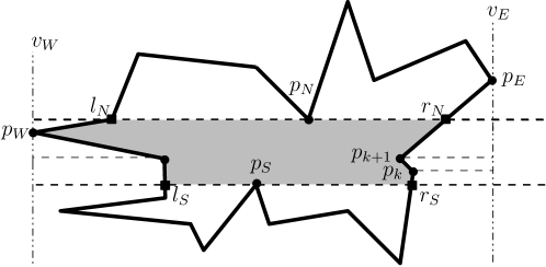
Figure 2: A $\{0^{\circ}\}$-${\rm Kernel}_{\theta}(P)$ for $\theta=0$.

Now, let $c^{l}$ and $c^{r}$ denote the left and the right polygonal chains defined, respectively, by those parts of the boundary of $P$ which are inside $S(P)$. Let $|c^{l}|$ and $|c^{r}|$ denote their number of segments. It follows from the definition of $S(P)$ and Lemma 6 that both chains are $0^{\circ}$-convex curves, i.e., $y$-monotone chains. See Figure 2 once more.

Corollary 8.

The area and the perimeter of the $\{0^{\circ}\}$-${\rm Kernel}(P)$ can be computed in $O(n)$ time.

Proof.

To compute the area of the $\{0^{\circ}\}$-${\rm Kernel}(P)=S(P)\cap P$ we proceed as follows. This area can be decomposed into (a finite number of) horizontal trapezoids defined by pairs of vertices in $c^{l}\cup c^{r}$ with consecutive $y$-coordinate. The area of these trapezoids can be computed in constant time, so the area of $\{0^{\circ}\}$-${\rm Kernel}(P)=S(P)\cap P$ can be computed in $O(|c^{l}|+|c^{r}|)$ time.

Computing the perimeter is even simpler, because we only need the addition of the lengths of $c^{l}$ and $c^{r}$ plus the lengths of the north and south boundaries of the $\{0^{\circ}\}$-${\rm Kernel}(P)$, which can also be done in $O(|c^{l}|+|c^{r}|)$ time. ∎

2.2 Computing and maintaining the $\{0^{\circ}\}$-${\rm Kernel}_{\theta}(P)$ of simple polygons

In this subsection, we show how to compute and maintain the $\{0^{\circ}\}$-${\rm Kernel}_{\theta}(P)$ as $\theta$ varies in $[-\frac{\pi}{2},\frac{\pi}{2})$, obtaining the intervals where it is non-empty, with the complexities in the first cell of the first row of Table 1. It is clear that we do not need a complete rotation, since $\{0^{\circ}\}$-${\rm Kernel}_{-\frac{\pi}{2}}(P)=\{0^{\circ}\}$-${\rm Kernel}_{\frac{\pi}{2}}(P)$. Also, observe that Definition 5, for reflex maxima/minima with respect to the horizontal orientation, can be easily extended to any orientation $\theta\in[-\frac{\pi}{2},\frac{\pi}{2})$ as follows.

Definition 9.

A reflex vertex $p_{i}$ in a simple polygon $P$ where $p_{i-1}$ and $p_{i+1}$ are both below (respectively above) $p_{i}$ with respect to a given orientation $\theta$ is a reflex maximum (resp. reflex minimum) with respect to $\theta$. Analogously, an edge of angle $\theta$ with two reflex vertices is a reflex maximum (resp. minimum) when its two neighbors are below (resp. above) with respect to the orientation $\theta$.

In order to know the intervals for $\theta$ such that the $\{0^{\circ}\}$-${\rm Kernel}_{\theta}(P)$ is not empty, we need to maintain the boundary of the rotation by angle $\theta$ of the strip $S(P)$ previously defined, which will be denoted as $S_{\theta}(P)$. It is straightforward to extend Lemma 6 to any orientation $\theta$. See Figure 3.

Lemma 10.

The $\{0^{\circ}\}$-${\rm Kernel}_{\theta}(P)$ is the region defined by the intersection $S_{\theta}(P)\cap P$.

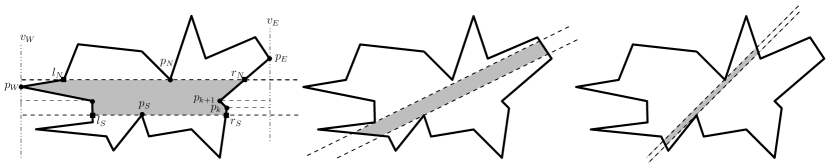
Figure 3: A rotating $\{0^{\circ}\}$-${\rm Kernel}_{\theta}(P)$ for $\theta=0$ (left), $\theta={\frac{\pi}{8}}$ (middle), and $\theta={\frac{\pi}{4}}$ (right).

Thus, in order to know when the $\{0^{\circ}\}$-${\rm Kernel}_{\theta}(P)$ is non-empty, we first need to maintain the equations of the two lines $h_{N}(\theta)$ and $h_{S}(\theta)$ passing through the lowest reflex minimum and the highest reflex maximum with respect to the current orientation $\theta$. Second, if we want to compute and maintain the boundary of $\{0^{\circ}\}$-${\rm Kernel}_{\theta}(P)$, we also need to maintain the set of vertices of the current left and right boundary chains, respectively denoted by $c^{l}_{\theta}$ and $c^{r}_{\theta}$, of $\{0^{\circ}\}$-${\rm Kernel}_{\theta}(P)$. See again Figure 3.

Now, we sketch an algorithm to compute the intervals of the values of $\theta$ within $[-\frac{\pi}{2},\frac{\pi}{2})$ such that $S_{\theta}(P)\not=\emptyset$ and therefore, such that $\{0^{\circ}\}$-${\rm Kernel}_{\theta}(P)\not=\emptyset$.

ALGORITHM FOR COMPUTING THE INTERVALS WITH $\{0^{\circ}\}$-${\rm Kernel}_{\theta}(P)\not=\emptyset$

1. For each vertex $p_{i}\in P$, check whether $p_{i}$ is reflex. If it is, compute the angular intervals $[\theta_{1}^{i},\theta_{2}^{i})$ and $[\theta_{1}^{i}+\pi,\theta_{2}^{i}+\pi)$ of orientations $\theta$ for which $p_{i}$ is reflex, and the corresponding reflex slope intervals defined when rotating with pivot $p_{i}$ the line containing the edge $p_{i-1}p_{i}$ up to the line containing the edge $p_{i}p_{i+1}$. Then, the vertex $p_{i}$ is a candidate to be a reflex maximum/minimum only for the orientations in the interval $[m_{1}^{i},m_{2}^{i})$. Note that a reflex slope interval may be split into two, in case it contains the orientation $\pi/2$.

2. From the information of Step 1, compute the sequence of event intervals, each of which is defined by a pair of orientation values $[\theta_{1},\theta_{2})\subset[-\frac{\pi}{2},\frac{\pi}{2})$ such that for any value $\theta\in(\theta_{1},\theta_{2})$ the strip $S_{\theta}(P)$ is supported by the same pair of vertices of $P$. In other words, such that the pair of vertices of $P$ defining the lowest reflex minimum and the highest reflex maximum does not change for $\theta\in(\theta_{1},\theta_{2})$. Recall Figure 3. Note that, by Lemma 6, the strip $S_{\theta}(P)$ is empty if, with respect to $\theta$, the lowest reflex minimum is below the highest reflex maximum. In order to compute the sequence of event intervals:

   Take the dual of the set of vertices $p_{i}\in P$, getting for each of them the line $D(p_{i})$. On each of these lines, mark the segment corresponding to the reflex slope interval of its primal point $p_{i}$. See Figure 4. Mark also all the line segments of the two polygonal chains corresponding to the dualization of the vertices of the upper and lower hulls of $CH(P)$.

   

   

   Figure 4: Dualization of a reflex slope interval.

   In this way, we get the set $\mathcal{D}$ with a linear number of straight-line segments in the dual plane, together with two polygonal chains. Now, sweeping a vertical line from left to right in the dual, the vertical corresponding to a value $\theta$ intersects some segments of the arrangement, which correspond to the reflex vertices in the primal. Since the dualization preserves the above-below relations between lines and/or points, the uppermost and the lowest segments intersected in the dual correspond in the primal to the lowest reflex minimum and the highest reflex maximum.

3. In $O(n\log n)$ time, compute the lower envelope of $\mathcal{D}$, denoted by $\mathcal{L_{\mathcal{D}}}$, and the upper envelope of $\mathcal{D}$, denoted by $\mathcal{U_{\mathcal{D}}}$ [6]. Sweeping in $O(n\log n)$ time the arrangement $\mathcal{L_{\mathcal{D}}}\cup\mathcal{U_{\mathcal{D}}}$ we obtain the sequence of pairs “lowest reflex minimum and highest reflex maximum” for all the event intervals $[\theta_{1},\theta_{2})$, as $\theta$ varies in $[-\frac{\pi}{2},\frac{\pi}{2})$. Since the upper envelope and the lower envelope of a set of $n$ possibly-intersecting straight-line segments in the plane have worst-case size $O(n\alpha(n))$, where $\alpha(n)$ is the extremely-slowly-growing inverse of Ackermann’s function [1], the number of pairs obtained is in $O(n\alpha(n))$.

4. Update an event interval $[\theta_{1},\theta_{2})\subseteq[-\frac{\pi}{2},\frac{\pi}{2})$ if, for the corresponding pair, the lowest reflex minimum is above the the highest reflex maximum.

5. Additionally, to maintain the polygonal chains $c^{l}_{\theta}$ and $c^{r}_{\theta}$ of the $\{0^{\circ}\}$-${\rm Kernel}_{\theta}(P)$, we compute the intersections of the lines $h_{N}(\theta)$ and $h_{S}(\theta)$ with the boundary of $P$, maintaining the information of the first and the last vertices of $c^{l}_{\theta}$ and $c^{r}_{\theta}$ in the current interval $[\theta_{1},\theta_{2})$.

From the discussion above, we get the following result.

Theorem 11.

For an $n$-vertex simple polygon $P$, there are $O(n\alpha(n))$ angular intervals $[\theta_{1},\theta_{2})\subset[-\frac{\pi}{2},\frac{\pi}{2})$ such that $\{0^{\circ}\}$-${\rm Kernel}_{\theta}(P)\not=\emptyset$ for all the values of $\theta\in[\theta_{1},\theta_{2})$, and the set of such intervals together with the boundary of $\{0^{\circ}\}$-${\rm Kernel}_{\theta}(P)$ can be computed and maintained in $O(n\log n)$ time and $O(n\alpha(n))$ space.

2.3 Optimizing the area and perimeter of the $\{0^{\circ}\}$-${\rm Kernel}_{\theta}(P)$ of simple polygons

2.3.1 Optimizing the area of the $\{0^{\circ}\}$-${\rm Kernel}_{\theta}(P)$

Let us consider the problem of optimizing the area of the $\{0^{\circ}\}$-${\rm Kernel}_{\theta}(P)$, i.e., computing the value(s) of $\theta$ such that the area of $\{0^{\circ}\}$-${\rm Kernel}_{\theta}(P)$ is maximum or minimum. We will prove the complexities in the second cell of the first row of Table 1.

First, subdivide the previous angular intervals $[\theta_{1},\theta_{2})$ every time that, as $\theta$ varies, a new vertex of the polygon $P$ enters the strip $S_{\theta}(P)$. Notice that this can be done in constant time, using the circular order of the vertices of $P$ and taking the smallest among the angles defined by the current points $p_{N}(\theta),h_{N}(\theta)$ (respectively $p_{S}(\theta),h_{S}(\theta)$) and the next two vertices of $P$ in the counterclockwise rotation of $h_{N}(\theta)$ (resp. $h_{S}(\theta)$). With a slight abuse of the notation, we will denote the angular intervals obtained after the subdivision with the same terminology as above, i.e., as $[\theta_{i},\theta_{i+1})$.

Then, at every step, the differential in the area can be decomposed into triangles, as shown in Figure 5. In particular, for each of these intervals $[\theta_{i},\theta_{i+1})$, within which the highest reflex maximum and the lowest reflex minimum do not change:

$$Area(\{0^{\circ}\}\text{-}{\rm Kernel}_{\theta_{i+1}}(P))=Area(\{0^{\circ}\}\text{-}{\rm Kernel}_{\theta_{i}}(P))+A_{1}+A_{2}-B_{1}-B_{2}.$$ (1)

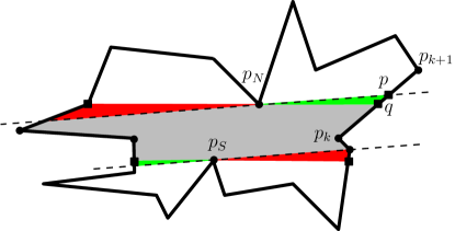
Figure 5: The four triangles $A_{1}$, $A_{2}$ (in green), and $B_{1}$, $B_{2}$ (in red).

Thus, the area of the $\{0^{\circ}\}$-${\rm Kernel}_{\theta}(P)$ can be expressed, using simple trigonometric relations, as a function $A(\beta)$ of the angle of rotation $\beta\in[\theta_{i},\theta_{i+1})$, see Section A.1 in the appendix. Then, it only remains to obtain the maximum value of that function in the interval. As detailed in Section A.1, this amounts to finding the real solutions of a polynomial equation in $t$ of degree $6$.

Before stating the algorithm to compute the optimal area, let us discuss the possible number of event intervals. Observe that events arise not only at changes of the lowest reflex minimum and the highest reflex maximum, but also when a new vertex of the polygon enters the strip, i.e., at changes in the polygonal chains $c^{l}_{\theta}$ and $c^{r}_{\theta}$ of $\{0^{\circ}\}$-${\rm Kernel}_{\theta}(P)$. Surprisingly enough, there can be a $\Theta(n^{2})$ number of these changes as shown in Figure 6. Thus, the number of event intervals is in $O(n^{2}\alpha(n))$.

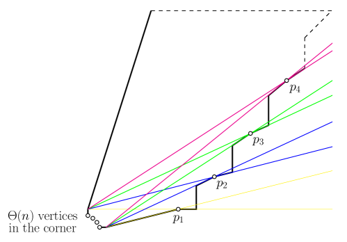
Figure 6: A point configuration such that for each vertex $p_{i}$, $1\leq i\leq 4$, all the $\Theta(n)$ vertices in the corner will be scanned again.

ALGORITHM FOR COMPUTING THE OPTIMAL AREA:

1. Let $[\theta_{1},\theta_{2})$ be the first event interval of the sequence of at most $O(n^{2}\alpha(n))$ event intervals. Let $p_{N}$ and $p_{S}$ be the corresponding lowest reflex minimum and highest reflex maximum. By Corollary 8, we can compute the value of the area $A(\theta_{1})$ of $\{0^{\circ}\}$-${\rm Kernel}_{\theta_{1}}(P)$ for the fixed orientation $\theta_{1}$ in $O(n)$ time and space. Then, we assign it as the first current area value.

2. According to the discussion above, compute the function $A(\beta)$, where $\beta\in[\theta_{1},\theta_{2})$, and in constant time determine the value of $\beta$ corresponding to the optimal area and update the maximum (and the minimum).

3. Proceed analogously with the next event interval, computing and updating in constant time the current optimal values for the area.

2.3.2 Optimizing the perimeter of $\{0^{\circ}\}$-${\rm Kernel}_{\theta}(P)$

Second, we consider the problem of optimizing the perimeter of $\{0^{\circ}\}$-${\rm Kernel}_{\theta}(P)$, denoted by $\Pi(\theta)$. We will prove the complexities in the third cell of the first row of Table 1.

The goal is to compute the value(s) of $\theta$ such that the perimeter of the $\{0^{\circ}\}$-${\rm Kernel}_{\theta}(P)$ is maximum (or minimum). The differential in the perimeter can be decomposed as adding two segments and subtracting two other segments, see Figure 7.

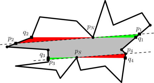
Figure 7: The relevant points for the computation of the optimal perimeter.

Again, the perimeter then can be expressed, using simple trigonometric relations, as a function $\Pi(\beta)$ of the angle of rotation $\beta\in[\theta_{i},\theta_{i+1})$, see Section A.2 in the appendix. Then, it only remains to obtain the maximum value of that function in the interval. As detailed in Section A.2, this amounts to finding the real solutions of a polynomial equation in $t$ of degree $35$.

Thus, an ALGORITHM FOR COMPUTING THE OPTIMAL PERIMETER analogous to the one proposed for the area at the end of Section 2.3.1 leads to the following result.

Theorem 12.

Given a simple polygon $P$ with $n$ vertices, the value of the angle $\theta\in[-\frac{\pi}{2},\frac{\pi}{2})$ such that the $\{0^{\circ}\}$-${\rm Kernel}_{\theta}(P)$ has maximum (and minimum) area and/or perimeter can be computed in $O(n^{2}\alpha(n))$ time and $O(n\alpha(n))$ space.

3 The rotated $\{0^{\circ},90^{\circ}\}$-${\rm Kernel}_{\theta}(P)$ of simple polygons

Next, we will study the problem of computing the $\mathcal{O}$-${\rm Kernel}$ of $P$ when $\mathcal{O}$ is given by two rotating perpendicular orientations, proving the results in the second row of Table 1. Notice that the two orientations do not need to be perpendicular for the proofs nor the algorithm in this section, because we are using Observation 3. Moreover, since the problem for a set $\mathcal{O}$ with $k$ orientations reduces to computing and maintaining the intersection of $k$ different kernels, the results in the third row of Table 1 will follow as well.

3.1 Computing and maintaining the $\{0^{\circ},90^{\circ}\}$-${\rm Kernel}_{\theta}(P)$ of simple polygons

From Observation 3, we can compute the $\{0^{\circ},90^{\circ}\}$-${\rm Kernel}_{\theta}(P)$ by computing the intersection of the two kernels $\{0^{\circ}\}$-${\rm Kernel}_{\theta}(P)$ and $\{90^{\circ}\}$-${\rm Kernel}_{\theta}(P)$. Note that, in fact, the latter equals $\{0^{\circ}\}$-${\rm Kernel}_{\theta+\frac{\pi}{2}}(P)$. In the following, the points $p_{W}$ and $p_{E}$ for the $\{90^{\circ}\}$-${\rm Kernel}_{\theta}(P)$ are analogous to the points $p_{N}$ and $p_{S}$ previously defined for the $\{0^{\circ}\}$-${\rm Kernel}_{\theta}(P)$, recall Figure 2.

The possible intersection shapes that arise during rotations are illustrated in Figures 8 and 9. In particular, notice the case in the right picture of the latter figure, where the intersection is just a rectangle.

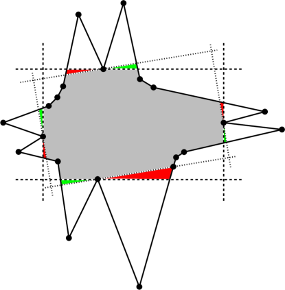
Figure 8: A general kernel and the rotated kernel in the next event.

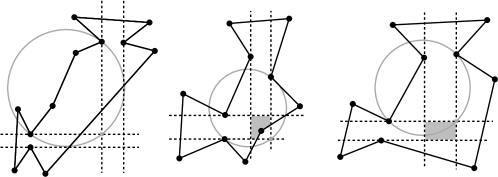
Figure 9: Three types of kernel.

Observe also that the kernel might be empty if: (i) one of the two kernels $\{0^{\circ}\}$-${\rm Kernel}_{\theta}(P)$ or $\{90^{\circ}\}$-${\rm Kernel}_{\theta}(P)$ is empty (then their intersection is also empty), or (ii) the intersection of both kernels is a rectangle lying outside the polygon $P$ (see Figure 9, left). The case (i) is easy to manage once we have computed the set of event intervals where each of the two kernels is non-empty. For the case (ii), assuming that we are working with event intervals where both $\{0^{\circ}\}$-${\rm Kernel}_{\theta}(P)$ and $\{90^{\circ}\}$-${\rm Kernel}_{\theta}(P)$ are non-empty, the following observation allows to check whether the intersection $\{0^{\circ}\}$-${\rm Kernel}_{\theta}(P)\cap\{90^{\circ}\}$-${\rm Kernel}_{\theta}(P)=\{0^{\circ},90^{\circ}\}$-${\rm Kernel}_{\theta}(P)$ is non-empty.

Observation 13.

The $\{0^{\circ},90^{\circ}\}$-${\rm Kernel}_{\theta_{i}}(P)$ is non-empty in the following cases: (a) At least one point among the current $p_{N}(\theta_{i})$ or $p_{S}(\theta_{i})$ is inside the kernel defined by $p_{E}(\theta_{i})$ and $p_{W}(\theta_{i})$, or vice versa (see Figure 8). (b) The polygon $P$ contains at least one of the corners of the rectangle given as the intersection of the (vertical) strip defined by two parallel lines $v_{W}(\beta)$ passing through $p_{W}(\theta_{i})$ with slope $\tan(\theta_{i}+\beta)$, and $v_{E}(\beta)$ passing through $p_{E}(\theta_{i})$ with slope $\tan(\theta_{i}+\beta)$, and the (horizontal) strip defined by the two parallel lines $h_{N}(\beta)$ passing through $p_{N}(\theta_{i})$ with slope $\tan(\theta_{i}+\pi/2+\beta)$, and $h_{S}(\beta)$ passing through $p_{S}(\theta_{i})$ with slope $\tan(\theta_{i}+\pi/2+\beta)$ (see Figure 9).

Thus, to compute and maintain the set of event intervals where $\{0^{\circ},90^{\circ}\}$-${\rm Kernel}_{\theta}(P)\not=\emptyset$ as $\theta\in[-\frac{\pi}{2},\frac{\pi}{2})$ we proceed with the following algorithm.

ALGORITHM FOR COMPUTING THE INTERVALS WITH $\{0^{\circ},90^{\circ}\}$-${\rm Kernel}_{\theta}(P)\not=\emptyset$:

1. Compute, in $O(n\log n)$ time and $O(n\alpha(n))$ space, the sequence of (at most $O(n\alpha(n))$) event intervals, say $[\theta_{i},\theta_{i+1})\subseteq[-\frac{\pi}{2},\frac{\pi}{2})$ where $\{0^{\circ}\}$-${\rm Kernel}_{\theta}(P)\not=\emptyset$. Proceed analogously to compute the sequence of event intervals, say $[\theta_{j},\theta_{j+1})\subseteq[-\frac{\pi}{2},\frac{\pi}{2})$ where $\{90^{\circ}\}$-${\rm Kernel}_{\theta}(P)\not=\emptyset$, in $O(n\log n)$ time and $O(n\alpha(n))$ space. In $O(n\alpha(n))$ time and space, merge these two event sequences into a sequence with complexity $O(n\alpha(n)$ of the event intervals corresponding to the simultaneous rotation of both kernels. Notice that, in fact, the second sequence is just the first one shifted by $\frac{\pi}{2}$.

2. We only have to care about the complexity of computing the intersection of both kernels at each event interval. For such an interval of a kernel, we compute and maintain the corresponding lowest reflex minimum and highest reflex maximum ($p_{N}$ and $p_{S}$ for the $\{0^{\circ}\}$-kernel, $p_{E}$ and $p_{W}$ for the $\{90^{\circ}\}$-kernel) and also the, at most four, points of $P$ which are the endpoints of the polygonal chains $c^{l}_{\theta_{i}}$ and $c^{r}_{\theta_{i}}$ say $p_{k_{1}}$, $p_{k_{2}}$, $p_{k_{3}}$, and $p_{k_{4}}$ for the $\{0^{\circ}\}$-${\rm Kernel}$ and $p^{\prime}_{k_{1}}$, $p^{\prime}_{k_{2}}$, $p^{\prime}_{k_{3}}$, and $p^{\prime}_{k_{4}}$ for the $\{90^{\circ}\}$-${\rm Kernel}$. The set of all these $12$ points does not change in the current event interval of both kernels.

3. From Observation 13, to determine the intervals where $\{0^{\circ},90^{\circ}\}$-${\rm Kernel}_{\theta}(P)\not=\emptyset$ we do the following for each of the intervals $[\theta_{i},\theta_{i+1})$ computed in the step 2:

   1. Check whether at least one point, $p_{N}$ or $p_{S}$, is inside the other kernel, defined by $p_{E}$ and $p_{W}$ (it is enough to check that it is inside the strip containing the other kernel), or vice versa. Notice that the situation of these four points cannot change during the event interval $[\theta_{i},\theta_{i+1})$. This can be checked in constant time, by an orientation test with the point considered and the two lines forming the strip.

   2. On the other case, we compute the four arcs of circles described by the four corners of the intersection rectangle of the two strips. See Figure 9, noting that each arc is defined by a corner of the rectangle and the two points among $\{p_{N},p_{W},p_{S},p_{E}\}$ corresponding to the two lines which define that corner. The corner $c_{ij}$ is the intersection point of the vertical line $v_{i}$ with the horizontal line $h_{j}$, $i\in\{N,S\},\,j\in\{W,E\}$. Notice that $v_{W}$ passes through $p_{W}$, $v_{E}$ passes through $p_{E}$, $h_{N}$ passes through $p_{N}$, and $h_{S}$ passes through $p_{S}$, respectively. For example, the point corner $c_{NE}$ describes the semicircle having as diameter the segment $\overline{p_{N}p_{E}}$; from this semicircle we compute the arc $a_{NE}$ corresponding to the current event interval $[\theta_{i},\theta_{i+1})$.

      Compute the intersection of each of the arcs $a_{ij}$ with the polygon $P$, splitting $a_{ij}$ into the sub-arcs which are inside $P$ in at most $O(n)$ time. Maintain the information of the sub-arcs or intervals while the corresponding pair does not change. Compute the union of the sub-arcs or its translation to event intervals where at least a corner is inside the current rectangle. Recall Figure 9. Because there are at most $O(n\alpha(n))$ pairs of lowest reflex minimum and highest reflex maximum (recall Section 2.2), the total complexity for this step will be $O(n^{2}\alpha(n))$.

The next result follows.

Theorem 14.

Given a simple polygon $P$ with $n$ vertices, there are at most $O(n^{2}\alpha(n))$ angular event intervals of the type $[\theta_{i},\theta_{i+1}]\subset[-\frac{\pi}{2},\frac{\pi}{2})$ such that $\{0^{\circ},90^{\circ}\}$-${\rm Kernel}_{\theta}(P)\not=\emptyset$ for all the values of $\theta\in[\theta_{i},\theta_{i+1})$. Moreover, the sequence of these intervals can be computed in $O(n^{2}\alpha(n))$ time and space.

It is clear that in case we have a set $\mathcal{O}=\{\alpha_{1},\dots,\alpha_{k}\}$ of $k$ orientations, we can extend Theorem 16. Notice that Observation 13 can be extended as follows: Instead of the four points $p_{N}$, $p_{S}$, $p_{E}$, and $p_{W}$, we have $2k$ highest/lowest reflex maxima/minima according to the $k$ different orientations. The extended version of condition (a) requires at least one of them to be inside the convex polygon defined by the intersection of the $k$ strips, what can be checked in $O(k)$ time and space, and condition (b) holds if at least a vertex of this convex polygon is inside $P$, what can be checked in $O(kn^{2}\alpha(n))$. Thus, we get the following.

Theorem 15.

Given a simple polygon with $n$ vertices, there are at most $O(kn^{2}\alpha(n))$ angular event intervals of the type $[\theta_{i},\theta_{i+1}]\subset[-\frac{\pi}{2},\frac{\pi}{2})$ such that $\{\alpha_{1},\dots,\alpha_{k}\}$-${\rm Kernel}_{\theta}(P)\not=\emptyset$ for all the values of $\theta\in[\theta_{i},\theta_{i+1})$. Moreover, the sequence of these intervals can be computed in $O(kn^{2}\alpha(n))$ time and space.

3.2 Optimizing the area and perimeter of $\{0^{\circ},90^{\circ}\}$-${\rm Kernel}_{\theta}(P)$ of simple polygons

To compute and maintain the optimal values for the area and perimeter of the $\{0^{\circ},90^{\circ}\}$-${\rm Kernel}_{\theta}(P)$, we can use the data computed above about the event intervals where this kernel is non-empty. Moreover, we can assume that in each of these intervals there are neither changes in the points of $P$ defining the kernel, nor changes in the vertices of the intersection rectangle of the two kernel strips. That is, following Observation 13, we compute different event intervals for the cases when one, two, three, or the four vertices of the rectangle lie inside the kernel. This only implies a multiplicative constant factor in the number of event intervals. Thus, again a total of $O(n^{2}\alpha(n))$ event intervals arise.

Next, we can analyze the method and formulas to compute the area or the perimeter according to the different types of event intervals. We can always assume that we have computed the area or the perimeter of the previous interval, i.e., if we are going to analyze the interval $[\theta_{i},\theta_{i+1})$ we know the values of the area and the perimeter for $[\theta_{i-1},\theta_{i})$.

Thus, for the area or perimeter in the case (a) of Observation 13, if these four points are inside the kernel, as in Figure 8, then we have to consider the $8$ triangles involved with the formulas for area or perimeter, in an analogous way as for the case of one orientation $\{0^{\circ}\}$-${\rm Kernel}_{\theta}(P)$ in Section 2.3. If there are three, two, or only one of the points inside the kernel, it is enough to incorporate the corresponding new formulas for these cases. For the sake of easier reading, and since the complexity of the algorithm does not increase, the details for those cases are omitted.

An analogous situation arises for the case (b) of Observation 13: If the rectangle contains the four corners inside the polygon $P$, then it is easy to describe the formulas for the area and perimeter. We would have to add new formulas for the cases where there are three, two, or only one corner of the rectangle, but again the complexity of the algorithm does not change and details are omitted.

Thus, it is clear that the relevant issue for the algorithms optimizing area or perimeter is the number $O(n^{2}\alpha(n))$ of event intervals, because the computations in each interval will be of constant time. Therefore, we have the following result.

Theorem 16.

Given a simple polygon with $n$ vertices, the values of $\theta\in[-\frac{\pi}{2},\frac{\pi}{2})$ such that the area or the perimeter of the $\{0^{\circ},90^{\circ}\}$-${\rm Kernel}_{\theta}(P)$ are maximum/minimum can be computed in $O(n^{2}\alpha(n))$ time and space.

4 Simple orthogonal polygons

In this section, we confine our study to simple orthogonal polygons, showing how the results in Table 1 can be improved to those in Table 2 for this case.

Each edge of an orthogonal polygon is a N-edge, S-edge, E-edge, or W-edge depending on whether it bounds the polygon from the north, south, east, or west, respectively. We call a sequence of alternating N- and E-edges a NE-staircase, and similarly we define the NW-staircase, SE-staircase, and SW-staircase. Clearly, each of these staircases is both $x$- and $y$-monotone (recall Figure 1). In addition, for $D\in\{{\rm N},{\rm S},{\rm E},{\rm W}\}$, a $D$-dent is a $D$-edge whose both endpoints are reflex vertices of the polygon.

Similarly, we can characterize the reflex vertices of an orthogonal polygon based on the type of incident edges. More specifically, each reflex vertex incident on a N-edge and an E-edge is called a NE-reflex vertex, and analogously we have the NW-, SE- and SW-reflex vertices. See Figure 10, left. This figure directly implies the following observation.

Observation 17.

With respect to the orientation $\theta$, for $\theta\in(0,\frac{\pi}{2})$, every SE-reflex vertex of an orthogonal polygon is a reflex maximum and every NW-reflex vertex is a reflex minimum, whereas for $\theta\in(\frac{\pi}{2},\pi)$, every SW-reflex vertex is a reflex maximum and every NE-reflex vertex is a reflex minimum. Analogously, with respect to the orientation $\theta+\frac{\pi}{2}$, for $\theta\in(0,\frac{\pi}{2})$, every SW-reflex vertex is a reflex maximum and every NE-reflex vertex is a reflex minimum, whereas for $\theta\in(\frac{\pi}{2},\pi)$, every SE-reflex vertex is a reflex maximum and every NW-reflex vertex is a reflex minimum.

Observation 17 indicates a crucial advantage of the orthogonal polygons over simple polygons. In an orthogonal polygon $P$, for any $\theta\in(0,\frac{\pi}{2})$ (and similarly for any $\theta\in(\frac{\pi}{2},\pi)$), the set of reflex minima/maxima does not change, and thus the lines bounding the strip $S_{\theta}(P)$ rotate in a continuous fashion, which directly implies that a situation like the one depicted in Figure 6 cannot occur. Additionally, since for a non-empty $\{0^{\circ}\}$-${\rm Kernel}_{\theta}(P)$, the lowest reflex minimum with respect to the orientation $\theta$ cannot be below the highest reflex maximum with respect to $\theta$, the observation implies the following corollary.

Corollary 18.

Let $P$ be a simple orthogonal polygon. If there are a SE-reflex vertex $u=(x_{u},y_{u})$ and a NW-reflex vertex $v=(x_{v},y_{v})$ of $P$ such that $x_{u}\leq x_{v}$ and $y_{u}\geq y_{v}$, then the $\{0^{\circ}\}$-${\rm Kernel}_{\theta}(P)$ is empty for each $\theta\in(0,\frac{\pi}{2})$; see Figure 10, right. Similarly, if there are a SW-reflex vertex $u=(x_{u},y_{u})$ and a NE-reflex vertex $v=(x_{v},y_{v})$ of $P$ such that $x_{u}\geq x_{v}$ and $y_{u}\geq y_{v}$, then the $\{0^{\circ}\}$-${\rm Kernel}_{\theta}(P)$ is empty for each $\theta\in(\frac{\pi}{2},\pi)$.

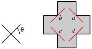
(a)

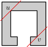
(b)

Figure 10: Left: The NW-reflex vertex $b$ and the SE-reflex vertex $d$ are a reflex minimum and a reflex maximum with respect to the orientation $\theta$, respectively, whereas the NE-reflex vertex $a$ and the SW-reflex vertex $c$ are a reflex minimum and a reflex maximum with respect to the orientation ${\theta}+\frac{\pi}{2}$, respectively. Right: Illustration for Corollary 18.

Notation.  We denote by $\vartheta_{P}(a,b)$ the counterclockwise (CCW) boundary chain of polygon $P$ from point $a$ to point $b$ where $a,b$ are located on the boundary of $P$.

4.1 The rotated $\{0^{\circ}\}$-${\rm Kernel}_{\theta}(P)$ of simple orthogonal polygons

We now prove the results in the first row of Table 2, focusing on the case for $\theta\in[0,\frac{\pi}{2})$ since the case for $\theta\in[-\frac{\pi}{2},0)$ is similar. Observation 17 implies that for $\theta\in(0,\frac{\pi}{2})$, only the SE-reflex (respectively NW-reflex) vertices contribute reflex maxima (resp. minima). We note that for $\theta=0$ (resp. $\theta=\frac{\pi}{2}$), the definition of $\{0^{\circ}\}$-visibility implies that only the S- and N-dents (resp. W- and E-dents) contribute reflex minima and maxima, respectively. As not all SE-reflex and NW-reflex vertices are corners of dents, there may be a discontinuity in the area or perimeter of the $\{0^{\circ}\}$-${\rm Kernel}_{\theta}(P)$ at $\theta=0$ and $\theta=\frac{\pi}{2}$; these two cases need to be treated separately.

Let $P$ be a simple orthogonal polygon. Let $u$ be the leftmost SE-reflex vertex of $P$ (in case of ties, take the topmost such vertex). Consider the downward-pointing ray $\vec{r}$ emanating from $u$ and, among its intersections with S-edges of $P$ extending to the left of $\vec{r}$, let $s_{SE}$ be the closest one to $u$. Similarly, let $u^{\prime}$ be the topmost SE-reflex vertex of $P$ (in case of ties, take the leftmost such vertex) and let $t_{SE}$ be, among the points of intersection of the rightward-pointing $\vec{r}\,^{\prime}$ emanating from $u^{\prime}$ with an E-edge extending above $\vec{r}\,^{\prime}$, the one closest to $u^{\prime}$; see Figure 11, left.

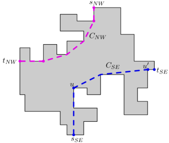
(a)

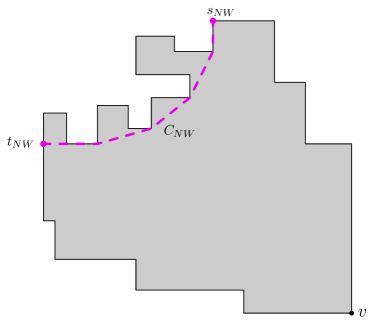
(b)

Figure 11: Left: An orthogonal polygon and the corresponding convex chains $C_{SE}$ and $C_{NW}$. Right: An orthogonal polygon without SE-reflex vertices in which we can consider that the convex chain $C_{SE}$ degenerates to vertex $v$.

Next, let $C_{SE}$ be the upper hull of the CCW boundary chain $\vartheta_{P}(s_{SE},t_{SE})$; see the blue dashed line in Figure 11, left. Similarly, by working with the NW-reflex vertices, we locate the (in case of ties, topmost) rightmost and the (in case of ties, leftmost) bottom-most NW-reflex vertices and we define the points $s_{NW}$ and $t_{NW}$, and the lower hull $C_{NW}$ of the CCW boundary chain $\vartheta_{P}(s_{NW},t_{NW})$. The chains $C_{SE}$ and $C_{NW}$ provide, respectively, the reflex maxima and minima during the rotation; the vertex of $C_{SE}$ (resp. $C_{NW}$) through which a tangent line to $C_{SE}$ (resp. $C_{NW}$) at an angle $\theta$ passes is precisely the reflex maximum (resp. minimum) with respect to the angle $\theta$. Thus, the bounding lines of the rotating strip $S_{\theta}(P)$ will be tangents to these hulls; see again Figure 11, left. We can also show the following result.

Lemma 19.

Let $P$ be a simple orthogonal polygon and let $s_{SE}$, $t_{SE}$, $C_{SE}$, $s_{NW}$, $t_{NW}$, and $C_{NW}$ be as defined earlier.

• Let $Q_{SE}$ be the convex part of the plane bounded from the left and above by $C_{SE}$, the downward-pointing ray emanating from $s_{SE}$, and the rightward-pointing ray emanating from $t_{SE}$. Similarly, let $Q_{NW}$ be the convex part of the plane bounded from the right and below by $C_{NW}$, the upward-pointing ray emanating from $s_{NW}$, and the leftward-pointing ray emanating from $t_{NW}$.

  • If the interiors of $Q_{SE}$ and $Q_{NW}$ intersect, then the $\{0^{\circ}\}$-${\rm Kernel}_{\theta}(P)$ is empty for each $\theta\in[0,\frac{\pi}{2})$.

  • If the interiors of $Q_{SE}$ and $Q_{NW}$ do not intersect but $Q_{SE}$ and $Q_{NW}$ touch at a common point $z$, then the $\{0^{\circ}\}$-${\rm Kernel}_{\theta}(P)$ degenerates to a line segment for each $\theta$ equal to the angle of each common interior tangent of $C_{SE}$ and $C_{NW}$ at $z$, and is empty for all other values of $\theta$.

  • If there exists a SE-reflex vertex not belonging to the CCW boundary chain $\vartheta_{P}(s_{SE},t_{SE})$ or a NW-reflex vertex not belonging to the CCW boundary chain $\vartheta_{P}(s_{SE},t_{SE})$, then the $\{0^{\circ}\}$-${\rm Kernel}_{\theta}(P)$ is empty for each $\theta\in(0,\frac{\pi}{2})$.

Proof.

(i) Let us concentrate on the case of a SE-reflex vertex of $P$, say $v$, not belonging to the CCW boundary chain $\theta_{P}(s_{SE},t_{SE})$. (The case of a NW-reflex vertex not belonging to the CCW boundary chain $\vartheta_{P}(s_{NW},t_{NW})$ is similar.) Since the chain $\vartheta_{P}(s_{SE},t_{SE})$ is determined by the leftmost and the topmost SE-reflex vertices, the $x$-coordinate of $v$ is larger than the $x$-coordinate of $s_{SE}$ and the $y$-coordinate of $v$ is smaller than the $y$-coordinate of $t_{SE}$. Moreover, if the bottom endpoint of the E-edge incident on $v$ is $w$ and the right endpoint of the S-edge incident on $v$ is $w^{\prime}$, then the order of these vertices along a CCW traversal of the boundary of $P$ is $t_{SE},w,v,w^{\prime},s_{SE}$.

It is important to note that the CCW boundary chain $\vartheta_{P}(t_{SE},w)$ of $P$ does not cross the upward-pointing vertical ray $\vec{r}$ emanating from $t_{SE}$, otherwise the leftmost vertex of the topmost edge of the CCW chain from $t_{SE}$ up to the first encountered crossing point to $\vec{r}$ is a SE-reflex vertex that is above $t_{SE}$, in contradiction to $t_{SE}$’s definition. Now, let $\vec{r}_{w}$ be the rightward-pointing horizontal ray emanating from $w$. Assume first that the chain $\vartheta_{P}(t_{SE},w)$ intersects the ray $\vec{r}_{w}$ at a point other than $w$; see Figure 12, left. Then, the right vertex of the bottommost horizontal edge (in $\vartheta_{P}(t_{SE},w)$) whose closure intersects the quadrant to the right and not above $w$ is a NW-reflex vertex (e.g., vertex $z$ in Figure 12, left). Since this vertex is below and to the right of the SE-reflex vertex $v$, Corollary 18 implies that the $\{0^{\circ}\}$-${\rm Kernel}_{\theta}(P)$ is empty for each $\theta\in(0,\frac{\pi}{2})$. Now, assume that the chain $\vartheta_{P}(t_{SE},w)$ does not intersect the ray $\vec{r}_{w}$ at a point other than $w$. If $q$ is the closest to $w$ intersection of $\vec{r}_{w}$ with the CCW boundary chain $\vartheta_{P}(s_{SE},t_{SE})$, then the closed polygonal line consisting of the CCW boundary chain $\vartheta_{P}(q,w)$ and the line segment $wq$ form a Jordan curve isolating vertex $v$ from $s_{SE}$. Hence, the ray $\vec{r}_{w}$ has to intersect the CCW boundary chain $\vartheta_{P}(w^{\prime},s_{SE})$ and let $p$ be the closest to $w$ such point of intersection; see Figure 12, right. Then, the bottom vertex of the rightmost vertical edge (in $\vartheta_{P}(w^{\prime},s_{SE})$) whose closure intersects the quadrant below and not to the left of $p$ is a NW-reflex vertex (e.g., vertex $z$ in Figure 12, right). Again, this vertex is below and to the right of the SE-reflex vertex $v$ and Corollary 18 implies that the $\{0^{\circ}\}$-${\rm Kernel}_{\theta}(P)$ is empty for each $\theta\in(0,\frac{\pi}{2})$.

(a)

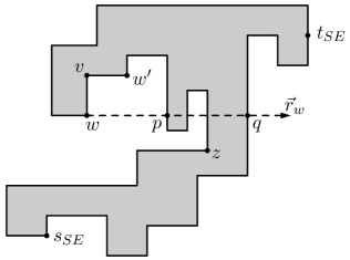
(b)

Figure 12: Figures for the proof of Lemma 19(i).

(ii.a) Let $p$ be a point in the intersection of the interiors of the unbounded convex polygons $Q_{SE}$ and $Q_{NW}$. Then, for any angle $\theta\in[0,\frac{\pi}{2})$, $p$ lies below the tangent to $C_{SE}$ at angle $\theta$ and above the tangent to $C_{NW}$ at angle $\theta$ and thus the strip $S_{\theta}(P)$ is empty. Therefore, by Lemma 6, the $\{0^{\circ}\}$-${\rm Kernel}_{\theta}(P)$ is empty for each $\theta\in[0,\frac{\pi}{2})$.

(ii.b) If $Q_{SE}$ and $Q_{NW}$ touch along their horizontal rays, then the $\{0^{\circ}\}$-${\rm Kernel}_{\theta}(P)$ is a horizontal line segment if $\theta=0$, otherwise it is empty. Similarly, if they touch along their vertical rays, then the $\{0^{\circ}\}$-${\rm Kernel}_{\theta}(P)$ is a vertical line segment if $\theta=\frac{\pi}{2}$, otherwise it is empty. Next, assume that $Q_{SE}$ and $Q_{NW}$ touch at a point of $C_{SE}$ and $C_{NW}$. Then, because $Q_{SE}$ and $Q_{NW}$ are convex, they touch at a connected portion of $C_{SE}$ and $C_{NW}$, that is, they touch at a point or a line segment. In either case, for any angle $\theta$ of any common interior tangent to $C_{SE}$ and $C_{NW}$, the $\{0^{\circ}\}$-${\rm Kernel}_{\theta}(P)$ is a line segment, otherwise it is empty. ∎

So, assume that none of the cases of Lemma 19 holds. Let $\phi_{1}$ and $\phi_{2}$ be the angles with respect to the positive $x$-axis of the common internal tangents to $C_{SE}$ and $C_{NW}$, with $\phi_{1}<\phi_{2}$. If the $y$-coordinate of $t_{NW}$ is greater than the $y$-coordinate of $t_{SE}$, then we set $\theta_{min}=0$, otherwise $\theta_{min}=\phi_{1}$. Similarly, we define $\theta_{max}$ to be equal to $\frac{\pi}{2}$ if the $x$-coordinate of $s_{SE}$ is greater than the $x$-coordinate of $s_{NW}$, otherwise $\theta_{max}=\phi_{2}$. For example, in Figure 11, left, $\theta_{min}=0$ and $\theta_{max}<\frac{\pi}{2}$. Then, since for $\theta\in[0,\frac{\pi}{2})$, the strip $S_{\theta}(P)$ is non-empty if and only if $\theta\in[\theta_{min},\theta_{max})$, by Lemma 6, we have:

Lemma 20.

Let $P$ be a simple orthogonal polygon and assume that none of the cases of Lemma 19 holds for $P$. Then, for $\theta\in(0,\frac{\pi}{2})$ the $\{0^{\circ}\}$-${\rm Kernel}_{\theta}(P)$ is non-empty if and only if $\theta\in[\theta_{min},\theta_{max})$.

Additionally, we can show:

Lemma 21.

Let $P$ be a simple orthogonal polygon, let $s_{SE}$, $t_{SE}$, $s_{NW}$, and $t_{NW}$ be as defined earlier, and suppose that there is an angle $\theta\in(0,\frac{\pi}{2})$ such that the $\{0^{\circ}\}$-${\rm Kernel}_{\theta}(P)$ is neither empty nor a line segment. Then, the CCW boundary chain $\vartheta_{P}(t_{NW},s_{SE})$ of $P$ from $t_{NW}$ to $s_{SE}$ is a SW-staircase and the CCW boundary chain $\vartheta_{P}(t_{SE},s_{NW})$ from $t_{SE}$ to $s_{NW}$ is a NE-staircase.

Proof.

Let us consider the case of the CCW boundary chain $\vartheta_{P}(t_{NW},s_{SE})$ (see Figure 11, left); the proof for the chain $\vartheta_{P}(t_{SE},s_{NW})$ is symmetric. Since there exist values of $\theta$ such that the $\{0^{\circ}\}$-${\rm Kernel}_{\theta}(P)$ is neither empty nor a line segment, Lemma 19(i) implies that no SE-reflex vertex exists that does not belong to the CCW boundary chain $\vartheta_{P}(s_{SE},t_{SE})$, and no NW-reflex vertex exists that does not belong to the CCW boundary chain $\vartheta_{P}(s_{NW},t_{NW})$. Thus, the chain $\vartheta_{P}(t_{NW},s_{SE})$ contains neither SE-reflex nor NW-reflex vertices.

Suppose that we start at the W-edge to which $t_{NW}$ belongs (let this edge be $uv$ with $v$ below $u$) and proceed in CCW order. The edge following the W-edge $uv$ is not a N-edge, otherwise the vertex $v$ would be a NW-reflex vertex, a contradiction. Thus, the edge following the W-edge $uv$ is a S-edge, let it be $vw$. If $s_{SE}\in vw$, then we are done and the lemma holds. Otherwise, if the edge following the edge $vw$ was an E-edge, then the top vertex of the leftmost edge in the CCW boundary chain $\vartheta_{P}(w,s_{SE})$ would be a SE-reflex vertex (note that the E-edge incident on $w$ belongs to this chain), a contradiction. Therefore, the edge following the S-edge $vw$ is a W-edge. Then, the above argument can be repeated until we reach the point $s_{SE}$, implying that the CCW boundary chain $\vartheta_{P}(t_{NW},s_{SE})$ is a NW-staircase. ∎

Lemma 21 implies that if the given polygon $P$ has no SE-reflex vertices, then the CCW boundary chain $\vartheta_{P}(t_{NW},s_{NW})$ consists of a SW-staircase followed by a NE-staircase; see Figure 11, right.

Based on Lemmas 19, 20, and 21, we now outline the algorithm to compute an angle $\theta\in[0,\frac{\pi}{2})$ such that the area (or perimeter) of the $\{0^{\circ}\}$-${\rm Kernel}_{\theta}(P)$ is maximized; minimization works similarly.

We start by computing points $s_{SE},\,t_{SE},\,s_{NW},\,t_{NW}$ and convex chains $C_{SE}$ and $C_{NW}$. We check whether the conditions of Lemma 19 hold and if they do, we handle these special cases as the lemma indicates. Otherwise, from the common internal tangents of $C_{SE}$ and $C_{NW}$, we compute $\theta_{min}$ and $\theta_{max}$. We start at $\theta=\theta_{min}$ and we explicitly compute the $\{0^{\circ}\}$-${\rm Kernel}_{\theta_{min}}(P)$ and its area (perimeter), which is the current area (perimeter) maximum.

(a)

(b)

Figure 13: Left: $\{0^{\circ}\}$-${\rm Kernel}_{\theta}(P)$ for $\theta=\phi$. Right: Computing the $\{0^{\circ}\}$-${\rm Kernel}_{\theta}(P)$ for $\theta\in[\phi,\phi^{\prime})$.

As in Section 2.3.1, we break the rotation into intervals, in each of which the kernel involves the same reflex minimum and maximum and the same edges of the polygon. Such an interval ends at the minimum angle in which either the current reflex maximum or minimum changes (i.e., it moves to the next vertex of the chains $C_{SE}$ or $C_{NW}$, respectively) or a vertex is encountered by one of the rotating parallel lines bounding the strip $S_{\theta}(P)$. In each such interval $[\theta_{i},\theta_{i+1})$, we maximize the area (perimeter) as a function of an angle $\beta\in[\theta_{i},\theta_{i+1})$ by taking into account the corresponding quantities of $\{0^{\circ}\}$-${\rm Kernel}_{\theta_{i}}(P)$ and of the two green triangles and the two red triangles in the spirit of Equation 1, as shown in Figure 13, right. The area (respectively perimeter) of each of these four triangles depends linearly on $\tan\beta$ or $\cot\beta$ (resp. linearly on $(1+\sin\beta)/\cos\beta$ or $(1-\cos\beta)/\sin\beta$); see Section A.3 in the appendix.

Computing the chains $C_{SE}$ and $C_{NW}$ can be done in $O(n)$ time [11]. Checking the conditions of Lemma 19 can also be done in $O(n)$ time (by traversing in lockstep fashion the chains $C_{SE}$ and $C_{NW}$, which are $x$-monotone), as can be done the computation of the angles $\theta_{min},\theta_{max}$. Computing the area (perimeter) of the kernel at the minimum angle $\theta_{min}$ takes $O(n)$ time. Now, suppose that we have $\beta=\theta_{i}$. Computing the angle $\theta_{i+1}$ as well as doing the maximization for the rotation interval $[\theta_{i},\theta_{i+1})$ takes constant time. Moreover, because the lines bounding $S_{\theta}(P)$ rotate in a continuous fashion, they slide monotonically along $C_{SE}$ and $C_{NW}$ and finish at points of the staircases from $t_{NW}$ to $s_{SE}$ and from $t_{SE}$ to $s_{NW}$, the number of such intervals is $O(n)$. Therefore:

Theorem 22.

Given a simple orthogonal polygon $P$, computing the $\{0^{\circ}\}$-${\rm Kernel}_{\theta}(P)$ as well as finding an angle $\theta$ such that its area (perimeter) is maximized or minimized can be done in linear time and space.

4.2 The rotated $\{0^{\circ},90^{\circ}\}$-${\rm Kernel}_{\theta}(P)$ of simple orthogonal polygons

We now extend our study to $\mathcal{O}=\{0^{\circ},90^{\circ}\}$ for the particular case of a simple orthogonal polygon $P$, proving the results in the second row of Table 2. Observe that it suffices to consider $\theta\in[0,\frac{\pi}{2})$ and note that $\{0^{\circ},90^{\circ}\}$-${\rm Kernel}_{0}(P)=\{0^{\circ},90^{\circ}\}$-${\rm Kernel}_{\frac{\pi}{2}}(P)$. The case for $\theta=0$ is treated as a special case and can be handled in linear time, and thus below we consider $\theta\in(0,\frac{\pi}{2})$.

The case is an extension of the $\{0^{\circ}\}$-${\rm Kernel}_{\theta}(P)$, now with two strips $S_{\theta}(P)$ and $S_{\theta+\frac{\pi}{2}}(P)$, that are perpendicular to each other, and the $\{0^{\circ},90^{\circ}\}$-${\rm Kernel}_{\theta}(P)$ is the intersection $P\,\cap\,S_{\theta}(P)\,\cap\,S_{\theta+\frac{\pi}{2}}(P)$. For $\theta\in(0,\frac{\pi}{2})$, in accordance with Observation 17, all reflex vertices are reflex maxima or minima with respect to one of the orientations in $\mathcal{O}_{\theta}$. Now, the definition of the $\{0^{\circ},90^{\circ}\}$-${\rm Kernel}_{\theta}(P)$ implies that:

Observation 23.

For $\theta\in(0,\frac{\pi}{2})$, the $\{0^{\circ},90^{\circ}\}$-${\rm Kernel}_{\theta}(P)$ is a convex polygon.

We note that for $\theta=0$, the $\{0^{\circ},90^{\circ}\}$-${\rm Kernel}_{\theta}(P)$ is not necessarily convex, but it is orthogonally convex. Since the kernel in this case is the intersection of the polygon $P$ with the horizontal strip determined above by the lowest N-dent and below by the topmost S-dent, and with the vertical strip determined to the left by the rightmost W-dent and to the right by the leftmost E-dent, there may be reflex vertices (but no dents) at the top left, top right, bottom left or bottom right corners.

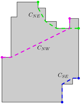
(a)

(b)

Figure 14: Left: A simple orthogonal polygon $P$ and the convex chains $C_{SE},C_{NE},C_{NW}$; no SW-reflex vertices exist. Right: The $\{0^{\circ},90^{\circ}\}$-${\rm Kernel}_{\theta}(P)$ for $\theta=\frac{\pi}{4}$ is shown darker.

As in the case of the $\{0^{\circ}\}$-${\rm Kernel}_{\theta}(P)$, we start by computing the convex chains $C_{SE}$, $C_{NE}$, $C_{NW}$ and $C_{SW}$ of the four types of reflex vertices (see Figure 14, left). Then, Lemma 19 implies:

Lemma 24.

If the conditions of Lemma 19 hold for either the pair $C_{SE}$ and $C_{NW}$, or the pair $C_{SW}$ and $C_{NE}$, then the $\{0^{\circ},90^{\circ}\}$-${\rm Kernel}_{\theta}(P)$ either is empty or degenerates to a line segment.

Thus, next we check whether the conditions of Lemma 19 hold for the pair $C_{SE}$ and $C_{NW}$, or the pair $C_{SW}$ and $C_{NE}$; if they do for at least one of these pairs, we handle this special case based on what the lemma suggests. Otherwise, from the common internal tangents of $C_{SE}$ and $C_{NW}$ and of $C_{SW}$ and $C_{NE}$, we compute $\theta_{min}$ and $\theta_{max}$. We start at $\theta=\theta_{min}$ and we explicitly compute the $\{0^{\circ},90^{\circ}\}$-${\rm Kernel}_{\theta_{min}}(P)$ and its area (perimeter), which is the current area (perimeter) maximum.

We proceed by considering angular intervals, so that in each of them (1) each of the strips $S_{\theta}(P)$ and $S_{\theta+\frac{\pi}{2}}(P)$ is determined by the same reflex minimum and maximum and (2) each endpoint of the segments bounding the strips does not move across a polygon vertex. So, at angle $\phi$, we determine the maximal such intervals $[\phi,\phi_{1})$ and $[\phi,\phi_{2})$ for the two strips and we consider the interval $[\phi,\min\{\phi_{1},\phi_{2}\})$. Moreover, this angular interval may need to be further broken into (as we shall see, a constant number of) subintervals as the segments bounding the strips may intersect inside the polygon (defining a vertex of the kernel) or not (in which case, an edge of the polygon contributes an edge of the kernel between the endpoints of the segments); see Figure 14, right.

To see this, consider an angle $\theta\in(0,\frac{\pi}{2})$ such that there is at least one reflex maximum in the orientation $\theta$ and at least one reflex minimum in the orientation $\theta+\frac{\pi}{2}$. Then, the strip $S_{\theta}(P)$ is bounded from below and the strip $S_{\theta+\frac{\pi}{2}}(P)$ is bounded from above; let $\ell_{{\theta},\downarrow}$ (resp. $\ell_{{90^{\circ}+\theta},\uparrow}$) be the bottom (resp. top) segment bounding $S_{\theta}(P)$ (resp. $S_{\theta+\frac{\pi}{2}}(P)$) and let $p$ (resp. $q$) be the right endpoint of $\ell_{{\theta},\downarrow}$ (resp. $\ell_{{90^{\circ}+\theta},\uparrow}$). Clearly $p$ belongs to a N- or an E-edge, and similarly, $q$ belongs to a S- or an E-edge. Each of the above possibilities for $p$ and $q$ may well arise if the segments $\ell_{{\theta},\downarrow}$ and $\ell_{{90^{\circ}+\theta},\uparrow}$ intersect (see Figure 15, left); the point of intersection lies in the polygon $P$ and, as the strips rotate, it moves along an arc of a circle whose diameter is the line segment connecting the reflex maximum and the reflex minimum about which $\ell_{{\theta},\downarrow}$ and $\ell_{{90^{\circ}+\theta},\uparrow}$, respectively, rotate. However, if these two segments do not intersect, then only one case for the relative location of $p$ and $q$ is possible, as we show in the following lemma.

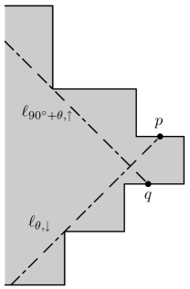
(a)

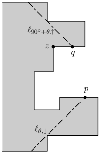
(b)

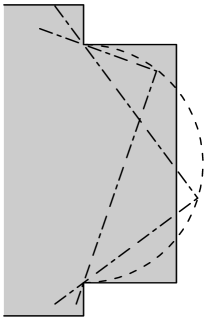
(c)

Figure 15: Left: The segments $\ell_{{\theta},\downarrow}$ and $\ell_{{90^{\circ}+\theta},\uparrow}$ intersect. Middle: For Lemma 25. Right: As the angle $\theta$ increases, the segments $\ell_{{\theta},\downarrow}$ and $\ell_{{90^{\circ}+\theta},\uparrow}$ intersect, later they stop doing so, and later they intersect again.

Lemma 25.

Let $P$ be a simple orthogonal polygon and suppose that the conditions of Lemma 19 hold neither for the pair $C_{SE}$ and $C_{NW}$, nor for the pair $C_{SW}$ and $C_{NE}$. Let segments $\ell_{{\theta},\downarrow}$ and $\ell_{{90^{\circ}+\theta},\uparrow}$ and points $p,q$ be defined as above. If $\ell_{{\theta},\downarrow}$ and $\ell_{{90^{\circ}+\theta},\uparrow}$ do not intersect, then $p$ and $q$ belong to the same E-edge of $P$.

Proof.

The tangency of the segments $\ell_{{\theta},\downarrow}$ and $\ell_{{90^{\circ}+\theta},\uparrow}$ to the chains $C_{SE}$ and $C_{NE}$, respectively, implies that $p,q$ belong (in fact, in that order) to the CCW boundary chain $\vartheta_{P}(t_{SE},s_{NE})$ of $P$. Suppose, for contradiction, that the point $p$ belongs to a N-edge. Then, no matter whether $q$ belongs to an E-edge or a S-edge, the left vertex of the topmost edge of the CCW boundary chain from $p$ to $q$ is a SE-reflex vertex that is higher than $p$ and thus higher than $t_{SE}$ (see vertex $z$ in Figure 15, middle), in contradiction to the assumption that Lemma 19, statement (ii), does not hold for the chain $C_{SE}$. Thus, $p$ belongs to an E-edge. The exact same argument enables us to show that $q$ belongs to an E-edge, and in fact that $p,q$ belong to the same E-edge. ∎

Since a circular arc (the locus of the intersection points of the lines supporting the rotating segments $\ell_{{\theta},\downarrow}$ and $\ell_{{90^{\circ}+\theta},\uparrow}$) and a line segment (e.g., an E-edge) intersect in at most two points, the above lemma implies that an angular interval $[\phi,\phi^{\prime})$, in which each of the strips $S_{\theta}(P)$ and $S_{\theta+\frac{\pi}{2}}(P)$ is determined by the same reflex minima and maxima and the same edges of the polygon $P$, may need to be broken into at most $12$ subintervals; indeed, it may be the case that in the interval $[\phi,\phi^{\prime})$, a pair of segments bounding the strips start by intersecting each other, then they stop doing so and later they start intersecting again (see Figure 15, right), and this may happen for all $4$ such pairs of bounding segments. Each of these subintervals is processed as explained in Section 4.1 for the case of the $\{0^{\circ}\}$-${\rm Kernel}_{\theta}(P)$; each case in which a pair of segments bounding the strips intersect each other contributes a term proportional to $\sin 2\theta$ in the area differential and a term proportional to $(\cos\theta+\sin\theta)$ in the perimeter differential as we show in Section A.4 in the appendix, whereas the contribution of the non-intersecting cases to the area and perimeter differential are as for the $\{0^{\circ}\}$-${\rm Kernel}_{\theta}(P)$.

The above discussion and the fact that the algorithm for the $\{0^{\circ},90^{\circ}\}$-${\rm Kernel}_{\theta}(P)$ is very similar to that for the $\{0^{\circ}\}$-${\rm Kernel}_{\theta}(P)$ lead to the following result.

Theorem 26.

Given a simple orthogonal polygon $P$, computing the $\{0^{\circ},90^{\circ}\}$-${\rm Kernel}_{\theta}(P)$ as well as finding an angle $\theta$ such that its area (perimeter) is maximized or minimized can be done in linear time and space.

Additionally, Lemma 25 readily implies that if the segments $\ell_{{\theta},\downarrow}$ and $\ell_{{90^{\circ}+\theta},\uparrow}$ do not intersect, then in the boundary of the $\{0^{\circ},90^{\circ}\}$-${\rm Kernel}_{\theta}(P)$ there exits a part of an edge of $P$ between $p$ and $q$. Note that the kernel has one fewer edge if $\ell_{{\theta},\downarrow}$ and $\ell_{{90^{\circ}+\theta},\uparrow}$ intersect or if exactly one of these segments is missing leaving the corresponding strip unbounded at one side; similar results hold for the remaining $4$ pairs of “consecutive” segments and more occurrences of the above cases result into a kernel of even fewer edges. Therefore:

Corollary 27.

For $\theta\neq 0,\frac{\pi}{2}$, the rotated $\{0^{\circ},90^{\circ}\}$-${\rm Kernel}_{\theta}(P)$ of an orthogonal polygon $P$ has at most $8$ edges.

Finally, since the problem for a set $\mathcal{O}$ with $k$ orientations is reduced to computing and maintaining the intersection of $k$ different kernels, the results in the third row of Table 2 follow.

Appendix A Appendix

A.1 Trigonometric formulas for Section 2.3.1

We label by $A_{1}$ and $A_{2}$ the areas of the two triangles given by the increase in the area produced by the variation of $\beta$ in $[\theta_{i},\theta_{i+1})$, depicted in green in Figure 5. Analogously, we label by $B_{1}$ and $B_{2}$ the areas of the two triangles we have to subtract to the current area, depicted in red in Figure 5.

We now deduce a formula for $A_{1}$. The other formulas for $A_{2}$, $B_{1}$, and $B_{2}$ can be obtained analogously. The coordinates of a point $p_{i}$ are denoted by $(x_{p_{i}},y_{p_{i}})$. The segment with endpoints $p$ and $q$ is denoted by $\overline{pq}$, its length is denoted by $|\overline{pq}|$, and the function $d(.,.)$ denotes the Euclidean distance between a point and a line. The area $A_{1}$ is

$$A_{1}=\frac{h}{2}|\overline{pq}|,$$

where $h$ can be calculated as the distance between the point $p_{N}$ and the line $\ell_{k}$ passing through the vertices $p_{k}$ and $p_{k+1}$, see Figure 16.

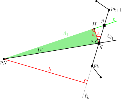
Figure 16: The triangle $A_{1}$ and the corresponding terminology.

The slope $m$ of this line $\ell_{k}$ is given by the formula

$$m=\frac{y_{p_{k+1}}-y_{p_{k}}}{x_{p_{k+1}}-x_{p_{k}}},$$

and the height $h$ is given by the formula

$$h=d(p_{N},\ell_{k})=\frac{|mx_{p_{N}}-y_{p_{N}}+y_{p_{K}}-mx_{p_{k}}|}{\sqrt{m^{2}+1}}.$$

Notice that the value $\frac{h}{2}$ is a constant, with respect to $\beta$, once we know $m$ and the coordinates of the points $p_{N}$ and $p_{k}$. Now we want to express the distance $|\overline{pq}|$ as a function of $\beta\in[\theta_{i},\theta_{i}+1)$, what can be done using some simple trigonometric relations, see again Figure 16. Note that from the picture, $|\overline{pq}|$ holds the relation $\cos\beta_{1}=\frac{h_{1}}{|\overline{pq}|}$, where $h_{1}=d(q,\ell)$. The point $q=(x_{q},y_{q})$ is known from the given value $\theta_{i}$. The line $\ell$ is determined by the point $p_{N}$ and the slope $\tan(\beta+\theta_{i})$, so it satisfies the equation

$$y-y_{p_{N}}=\tan(\beta+\theta_{i})(x-x_{p_{N}}).$$

Therefore,

$$h_{1}=\frac{|\tan(\beta+\theta_{i})x_{q}-y_{q}+y_{P_{N}}-\tan(\beta+\theta_{i})x_{P_{N}})|}{\sqrt{\tan^{2}(\beta+\theta_{i})+1}}.$$

By the trigonometric relation $\tan^{2}(\beta+\theta_{i})+1=\frac{1}{\cos^{2}(\beta+\theta_{i})}$, we get that

$$h_{1}=\pm[C\sin\beta+D\cos\beta],$$

where $C$ and $D$ are constants in the current event interval: $C=(x_{q}-x_{p_{N}})\cos\theta_{i}-(y_{p_{N}}-y_{q})\sin\theta_{i}$ and $D=(x_{q}-x_{p_{N}})\sin\theta_{i}+(y_{p_{N}}-y_{q})\cos\theta_{i}$.

On the other hand, from the relation $\alpha_{1}-\beta_{1}+\beta=\frac{\pi}{2}$ (see Figure 16) we derive that

$$\begin{array}[]{rll}\cos\beta_{1}&=&\cos[(\alpha_{1}-\frac{\pi}{2})+\beta]\\ &=&\sin\alpha_{1}\cos\beta+\cos\alpha_{1}\sin\beta.\end{array}$$

Next, let us denote $E=\sin\alpha_{1}$ and $F=\cos\alpha_{1}$ and notice that this values are constants because the angle $\alpha_{1}$ is computed from the points $p_{N}$, $q$, and $p_{k}$. Thus,

$$|\overline{pq}|=\frac{\pm[C\sin\beta+D\cos\beta]}{\sin\alpha_{1}\cos\beta+\cos\alpha_{1}\sin\beta}$$ (2)

and then

$$A_{1}=\pm\frac{h(C\sin\beta+D\cos\beta)}{2(E\cos\beta+F\sin\beta)}.$$

Now, we will use the length of the segment $pq$ for the computation of both the area and the perimeter. Namely, using Equation 1 and the computations above, we can write

$$A(\beta)=A(\theta_{i})+(A_{1}+A_{2}-B_{1}-B_{2})=\displaystyle A(\theta_{1})+\sum_{i=1}^{4}\frac{C_{i}\sin\beta+D_{i}\cos\beta}{E_{i}\sin\beta+F_{i}\cos\beta},$$

where $A(\theta_{i})$ (the value of the current area), $C_{i}$, $D_{i}$, $E_{i}$, and $F_{i}$ are all constants for every $i=1,\dots,4$. Then, doing the derivatives equal to zero, we get

$$A^{\prime}(\beta)=\displaystyle\sum_{i=1}^{4}\frac{C_{i}F_{i}-D_{i}E_{i}}{(E_{i}\sin\beta+F_{i}\cos\beta)^{2}}=0,$$

implying that

$$\sum_{i=1}^{4}\left[(C_{i}F_{i}-D_{i}E_{i})\prod_{\begin{subarray}{c}{j=1}\\ {j\neq i}\end{subarray}}^{4}(E_{j}\sin\beta+F_{j}\cos\beta)^{2}\right]=0.$$

Expanding the product, we find three types of terms depending on $\sin^{2}\beta$, $\cos^{2}\beta$, and $\sin\beta\cos\beta$. Now using the trigonometric transformations

$$\sin^{2}\beta=\frac{\tan^{2}\beta}{1+\tan^{2}\beta},\quad\cos^{2}\beta=\frac{1}{1+\tan^{2}\beta},\quad\text{ and }\quad\sin\beta\cos\beta=\pm\frac{\tan\beta}{1+\tan^{2}\beta},$$

and making the change $\tan\beta=t$ we get a rational function in $t$. Then, the derivative function for the area is now a function on the variable $t$, $A^{\prime}(t)$, and it is a rational function having as numerator a polynomial in $t$ of degree $6$ and as denominator a polynomial of degree $12$. So we can compute the real solutions of a polynomial equation in $t$ of degree $6$.

A.2 Trigonometric formulas for Section 2.3.2

We shall make use of some of the previous formulas. In the next formulas the points $q_{1}$, $q_{2}$, $q_{3}$, and $q_{4}$ are the intersection points of the lines $h_{N}(\theta_{i})$ and $h_{S}(\theta_{i})$ with the polygon $P$ (whose coordinates have been computed in the previous event interval), and the points $p_{1}$, $p_{2}$, $p_{3}$, and $p_{4}$ are the intersection points of the lines $h_{N}(\theta_{i}+\beta)$ and $h_{S}(\theta_{i}+\beta)$ with the polygon $P$ in the event interval $[\theta_{i},\theta_{i+1})$, see Figure 7.

$$\begin{split}\displaystyle\Pi(\beta)&:=\Pi(\theta_{i})+\displaystyle\sum_{i=1}^{4}(-1)^{i+1}|\overline{p_{i}q_{i}}|+\sum_{i=1}^{2}(|\overline{p_{i}p_{N}}|-|\overline{q_{i}p_{N}}|)+\sum_{i=3}^{4}(|\overline{p_{i}p_{S}}|-|\overline{q_{i}p_{S}}|)\\ &=\displaystyle\left[\Pi(\theta_{i})-\sum_{i=1}^{2}|\overline{q_{i}p_{N}}|-\sum_{i=3}^{4}|\overline{q_{i}p_{S}}|\right]+\displaystyle\left[\sum_{i=1}^{4}(-1)^{i+1}|\overline{p_{i}q_{i}}|\right]+\left[\sum_{i=1}^{2}|\overline{p_{i}p_{N}}|+\sum_{i=3}^{4}|\overline{p_{i}p_{S}}|\right].\end{split}$$ (3)

In the formula above, the first term between brackets is a constant since the values of $|\overline{q_{i}p_{N}}|$ and $|\overline{q_{i}p_{S}}|$ can be obtained in constant time from the former event interval, or computed also in constant time for the initial event interval; for the second term between brackets, the four values of $|\overline{p_{i}q_{i}}|$, $i\in\{1,2,3,4\}$, can be computed analogously to the formula for $|\overline{pq}|$ in Equation 2; the third term between brackets involves the values of $|\overline{p_{i}p_{N}}|$ and $|\overline{p_{i}p_{S}}|$, whose computations are clearly similar to the computation of $|\overline{pp_{N}}|$ (see Figure 16), that we do next.

From Figure 7, $|\overline{pp_{N}}|=|\overline{pH}|+|\overline{Hp_{N}}|$, where $|\overline{pH}|$ and $|\overline{Hp_{N}}|$ hold the relations $\sin\beta_{1}=\frac{|\overline{pH}|}{|\overline{pq}|}$ and $\cos\beta=\frac{|\overline{Hp_{N}}|}{|\overline{qp_{N}}|}$, respectively. Therefore

$$|\overline{pp_{N}}|=|\overline{pq}|\sin\beta_{1}+|\overline{qp_{N}}|\cos\beta.$$

Now, using the expression for $|\overline{pq}|$ in Equation 2 and the fact that $G=qp_{N}$ is a constant in the current interval, we can write

$$|\overline{pp_{N}}|=\frac{C\sin\beta+D\cos\beta}{\cos\beta_{1}}\sin\beta_{1}+G\cos\beta=(C\sin\beta+D\cos\beta)\tan\beta_{1}+G\cos\beta.$$

Then, since $\beta_{1}=\alpha_{1}-\frac{\pi}{2}+\beta$, we get

$$|\overline{pp_{N}}|=(C\sin\beta+D\cos\beta)\frac{J+\tan\beta}{1-J\tan\beta}+G\cos\beta,$$

where $J=\tan\left(\alpha_{1}-\frac{\pi}{2}\right)$ is a constant.

Thus, $|\overline{p_{i}p_{N}}|$, for $i=1,2$, and $|\overline{p_{i}p_{S}}|$, for $i=3,4$, admit analogous expressions

$$(C_{i}\sin\beta+D_{i}\cos\beta)\frac{J_{i}+\tan\beta}{1-J_{i}\tan\beta}+G_{i}\cos\beta.$$

Putting all the former observations together, we obtain from Equation 3 the following formula for the perimeter as a function of the rotation angle $\beta$:

$$\Pi(\beta)=O(1)+\displaystyle\sum_{i=1}^{4}\left[\frac{C_{i}\sin\beta+D_{i}\cos\beta}{E_{i}\sin\beta+F_{i}\cos\beta}+(C_{i}\sin\beta+D_{i}\cos\beta)\frac{J_{i}+\tan\beta}{1-J_{i}\tan\beta}+G_{i}\cos\beta\right].$$ (4)

In order to simplify the next computations, we make the change of variables $\tan\frac{\beta}{2}=t$ in Equation 4. It is straightforward to see that $\sin\beta=\frac{2t}{1+t^{2}}$, $\cos\beta=\frac{1-t^{2}}{1+t^{2}}$ and $\tan\beta=\frac{2t}{1-t^{2}}$ and then

$$\Pi(t)=O(1)+\displaystyle\sum_{i=1}^{4}\left[\frac{2C_{i}t+D_{i}(1-t^{2})}{2E_{i}t+F_{i}(1-t^{2})}+\frac{2C_{i}t+D_{i}(1-t^{2})}{1+t^{2}}\frac{2t+J_{i}(1-t^{2})}{1-2J_{i}t-t^{2}}+G_{i}\frac{1-t^{2}}{1+t^{2}}\right].$$

The derivative function of the perimeter, $\Pi^{\prime}(\beta)$, is now a rational function in $t$ whose numerator is a polynomial in $t$ of degree $35$.

A.3 Trigonometric formulas for Section 4.1

We only need to compute the area and the perimeter of a triangle with a horizontal or a vertical base in terms of $\beta\in[\theta_{i},\theta_{i+1}]\subseteq(0,\frac{\pi}{2})$.

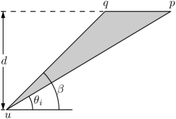
(a)

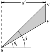
(b)

Figure 17: For the formulas of the area and perimeter of the $\{0^{\circ}\}$-${\rm Kernel}_{\theta}$ of orthogonal polygons.

From Figure 17 (left), the area of a triangle with edges at angles $0$ (horizontal edge), $\theta_{i}$, and $\beta$ ($0<\theta_{i}\leq\beta\leq\theta_{i+1}<\frac{\pi}{2}$) is equal to

$$A\ =\ \frac{1}{2}\,d\ |\overline{pq}|\ =\ \frac{1}{2}\,d\,(d\cot\theta_{i}-d\cot\beta)\ =\ \frac{1}{2}\,d^{2}\,(\cot\theta_{i}-\cot\beta).$$

In turn, no matter whether the kernel increases or decreases by such a triangle, the absolute value of the differential $\Delta\Pi$ in the perimeter is equal to the sum of the lengths of the triangle sides at angles $0$ and $\beta$ minus the length of the side at angle $\theta_{i}$. Thus:

$$\Delta\Pi = |\overline{uq}|+|\overline{pq}|-|\overline{up}|\ =\ \frac{d}{\sin\beta}+(d\cot\theta_{i}-d\cot\beta)-\frac{d}{\sin\theta_{i}}$$

$$= d\left(\frac{1}{\sin\beta}+\frac{\cos\theta_{i}}{\sin\theta_{i}}-\frac{\cos\beta}{\sin\beta}-\frac{1}{\sin\theta_{i}}\right)\ =\ d\left(\frac{1-\cos\beta}{\sin\beta}-\frac{1-\cos\theta_{i}}{\sin\theta_{i}}\right).$$

Analogously (see Figure 17, right), the area of a triangle with edges at angles $\frac{\pi}{2}$ (vertical edge), $\theta_{i}$, and $\beta$ ($0<\theta_{i}\leq\beta\leq\theta_{i+1}<\frac{\pi}{2}$) is equal to

$$A\ =\ \frac{1}{2}\,d^{\prime}\,|\overline{pq}|\ =\ \frac{1}{2}\,d^{\prime}\,(d^{\prime}\tan\beta-d^{\prime}\tan\theta_{i})\ =\ \frac{1}{2}\,(d^{\prime})^{2}\,(\tan\beta-\tan\theta_{i}).$$

For the differential $\Delta\Pi$ in the perimeter, we have:

$$\Delta\Pi = |\overline{uq}|+|\overline{pq}|-|\overline{up}|\ =\ \frac{d^{\prime}}{\cos\beta}+(d^{\prime}\tan\beta-d^{\prime}\tan\theta_{i})-\frac{d^{\prime}}{\cos\theta_{i}}$$

$$= d^{\prime}\left(\frac{1}{\cos\beta}+\frac{\sin\beta}{\cos\beta}-\frac{\sin\theta_{i}}{\cos\theta_{i}}-\frac{1}{\cos\theta_{i}}\right)\ =\ d^{\prime}\left(\frac{1+\sin\beta}{\cos\beta}-\frac{1+\sin\theta_{i}}{\cos\theta_{i}}\right).$$

Thus, the area $A(\beta)$ of the $\{0^{\circ}\}$-${\rm Kernel}_{\theta}(P)$ in terms of $\beta\in[\theta_{i},\theta_{i+1})$ is equal to

$$A(\beta)=A(\theta_{i})+C\,(\cot\theta_{i}-\cot\beta)+C^{\prime}\,(\tan\beta-\tan\theta_{i})$$

for appropriate constants $C,C^{\prime}$. Since $\theta_{i}$ is fixed, we need to maximize/minimize an expression of the form

$$f_{A}(\beta)=c_{1}\tan\beta+c_{2}\cot\beta+c_{3}$$

for $\beta\in[\theta_{i},\theta_{i+1})$ and constants $c_{1},c_{2},c_{3}$.

Similarly, the perimeter $\Pi(\beta)$ of the $\{0^{\circ}\}$-${\rm Kernel}_{\theta}(P)$ in terms of $\beta\in[\theta_{i},\theta_{i+1})$ is equal to

$$\Pi(\beta)=\Pi(\theta_{i})+D\,\left(\frac{1-\cos\beta}{\sin\beta}-\frac{1-\cos\theta_{i}}{\sin\theta_{i}}\right)+D^{\prime}\,\left(\frac{1+\sin\beta}{\cos\beta}-\frac{1+\sin\theta_{i}}{\cos\theta_{i}}\right)$$

for appropriate constants $D,D^{\prime}$. Since $\theta_{i}$ is fixed, we need to maximize/minimize an expression of the form

$$f_{\Pi}(\beta)=c^{\prime}_{1}\frac{1-\cos\beta}{\sin\beta}+c^{\prime}_{2}\frac{1+\sin\beta}{\cos\beta}+c^{\prime}_{3}$$

for $\beta\in[\theta_{i},\theta_{i+1})$ and constants $c^{\prime}_{1},c^{\prime}_{2},c^{\prime}_{3}$.

The maximization/minimization of $f_{A}(\beta)$ and $f_{\Pi}(\beta)$ can be done with standard techniques using the derivative of these functions.

A.4 Trigonometric formulas for Section 4.2

If the segments bounding the two strips do not intersect, then we get triangles as those in Section A.3, contributing terms proportional to $\tan\beta$, $\cot\beta$, and constant for the area, and to $\frac{1-\cos\beta}{\sin\beta}$, $\frac{1+\sin\beta}{\cos\beta}$, and constant for the perimeter, where $\beta\in[\theta_{i},\theta_{i+1}]\subseteq(0,\frac{\pi}{2})$.

Figure 18: For the formulas of the area and perimeter of the $\{0^{\circ},90^{\circ}\}$-${\rm Kernel}_{\theta}(P)$ of orthogonal polygons.

Let us now consider the case in which the kernel is bounded by intersecting segments $s_{u}$ and $s_{v}$ through pivoting vertices $u$ and $v$, respectively; hence, the point of intersection lies in $P$ and if this is so for all the angles $\beta\in[\theta_{i},\theta_{i+1})$, then the corner of the kernel moves along a circular arc with diameter the length of the segment $\overline{uv}$; see Figure 18. Then, the differential in the area is

$$\Delta A = A(\overset{\triangle}{uvq})-A(\overset{\triangle}{uvp})\ =\ \frac{1}{2}\,|\overline{uq}|\,|\overline{vq}|-\frac{1}{2}\,|\overline{up}|\,|\overline{vp}|$$

$$= \frac{1}{2}\,(|\overline{uv}|\,\cos\beta)\,(|\overline{uv}|\,\sin\beta)-\frac{1}{2}\,(|\overline{uv}|\,\cos\theta_{i})\,(|\overline{uv}|\,\sin\theta_{i})$$

$$= \frac{1}{2}\,|\overline{uv}|^{2}\,\sin\beta\,\cos\beta-\frac{1}{2}\,|\overline{uv}|^{2}\,\sin\theta_{i}\,\cos\theta_{i}$$

$$= \frac{1}{4}\,|\overline{uv}|^{2}\,(\sin 2\beta-\sin 2\theta_{i}).$$

In a similar fashion, the differential in the perimeter is

$$\Delta\Pi = (|\overline{uq}|+|\overline{vq}|)-(|\overline{up}|+|\overline{vp}|)$$

$$= (|\overline{uv}|\,\cos\beta+|\overline{uv}|\,\sin\beta)-(|\overline{uv}|\,\cos\theta_{i}+|\overline{uv}|\,\sin\theta_{i})$$

$$= |\overline{uv}|\,(\cos\beta+\sin\beta)-|\overline{uv}|\,(\cos\theta_{i}+\sin\theta_{i}).$$

References

- [1] W. Ackermann. Zum Hilbertschen Aufbau der reellen Zahlen. Mathematische Annalen, 99, 1928, 118–133.
- [2] S. W. Bae. Geodesic farthest neighbors in a simple polygon and related problems. 27th International Symposium on Algorithms and Computation (ISAAC 2016), 14.1–14.12.
- [3] G. S. Brodal and R. Jacob. Dynamic Planar Convex Hull. Proceedings of the 43rd Annual IEEE Symposium on Foundations of Computer Science, 2002.
- [4] L.P. Gewali. Recognizing -Star Polygons. Pattern Recognition, 28(7), 1995, 1019–1032.
- [5] E. Fink and D. Wood. Restricted-orientation convexity. Monographs in Theoretical Computer Science, An EATCS Series, Springer-Verlag, 2004.
- [6] J. Hershberger. Finding the upper envelope of line segments in time. Information Processing Letters, 33(4), 1989, 169–174.
- [7] G. Huskić, S. Buck, and A. Zell. GeRoNa: Generic robot navigation. Journal of Intelligent & Robotic Systems, 95(2), 2019, 419–442.
- [8] C. Icking and R. Klein. Searching for the kernel of a polygon: A competitive strategy. Proceedings of the 11th Annual Symposium on Computational Geometry, 1995, 258–266.
- [9] Y. Ke and J. O’Rourke. Computing the kernel of a point set in a polygon. Lecture Notes in Computer Science, vol. 382, (1989), 135–146.
- [10] D. T. Lee and F. P. Preparata. An Optimal Algorithm for Finding the Kernel of a Polygon. Journal of the ACM, 26(3), 1979, 415–421.
- [11] A. Melkman, On-line construction of the convex hull of a simple polygon, Information Processing Letters 25 (1987), 11–12.
- [12] L. Palios. An output-sensitive algorithm for computing the -kernel. 27th Canadian Conference on Computational Geometry, Kingston, 2015, 199–204.
- [13] L. Palios. A New Competitive Strategy for Reaching the Kernel of an Unknown Polygon. Lecture Notes in Computer Science, vol. 1851, (2000), 367–382.
- [14] G. J. E. Rawlins, and D. Wood. Optimal computation of finitely oriented convex hulls. Information and Computation 72, (1987), 150–166.
- [15] S. Schuierer, G. J. E. Rawlins, and D. Wood. A generalization of staircase visibility. 3rd Canadian Conference on Computational Geometry, Vancouver, 1991, 96–99.
- [16] S. Schuierer and D. Wood. Generalized kernels of polygons with holes. 5th Canadian Conference on Computational Geometry, Waterloo, 1993, 222–227.
- [17] S. Schuierer and D. Wood. Multiple-guards kernels of simple polygons. Theoretical Computer Science Center Research Report HKUST-TCSC-98-06, 1998.
- [18] K. Sugihara and J. Smith. Genetic algorithms for adaptive motion planning of an autonomous mobile robot. Proceedings of the IEEE International Symposium on Computational Intelligence in Robotics and Automation, 1997, 138–143.