Dynamics of a prey-predator system with modified Leslie-Gower and Holling type II schemes incorporating a prey refuge

Abstract

We study a modified version of a prey-predator system with modified Leslie-Gower and Holling type II functional responses studied by M.A. Aziz-Alaoui and M. Daher-Okiye. The modification consists in incorporating a refuge for preys, and substantially complicates the dynamics of the system. We study the local and global dynamics and the existence of cycles. We also investigate conditions for extinction or existence of a stationary distribution, in the case of a stochastic perturbation of the system.

Safia Slimani

Normandie Univ, Laboratoire Raphaël Salem

UMR CNRS 6085, Rouen, France

Paul Raynaud de Fitte and Islam Boussaada

Normandie Univ, Laboratoire Raphaël Salem,

UMR CNRS 6085, Rouen, France.

PSA $\&$ Inria DISCO $\&$ Laboratoire des Signaux et Systèmes,

Université Paris Saclay, CNRS-CentraleSupélec-Université Paris Sud,

3 rue Joliot-Curie, 91192 Gif-sur-Yvette cedex, France

Keywords: Prey-predator, Leslie-Gower, Holling type II, refuge, Poincaré index theorem, stochastic differential, persistence, stationary distribution, ergodic.

1 Introduction

We study a two-dimensional prey-predator system with modified Leslie-Gower and Holling type II functional responses. This system is a generalization of the system investigated in the papers by M.A. Aziz-Alaoui and M. Daher-Okiye [3, 9].

Aziz-Alaoui and Daher-Okiye’s model has been studied and generalized in numerous papers: models with spatial diffusion term [6, 33, 2, 1], with time delay [29, 35, 34], with stochastic perturbations [25, 24, 27, 22], or incorportaing a refuge for the prey [7], to cite but a few.

A novelty of the present paper is that we add a refuge in a way which is different from [7], since the density of prey in our refuge is not proportional to the total density of prey. This kind of refuge entails a qualitatively different behavior of the solutions, even for a small refuge, contrarily to the type of refuge investigated in [7]. Let us emphasize that, even in the case without refuge, our study provides new results.

In the first and main part of the paper (Section 2), we study the system of [3, 9] with refuge, but without stochastic perturbation:

(1.1) $$\left\{\begin{aligned} &\dot{\textrm{\bf x}}=\textrm{\bf x}(\rho_{1}-\beta\textrm{\bf x})-\frac{\alpha_{1}\textrm{\bf y}(\textrm{\bf x}-\mu)_{+}}{\kappa_{1}+(\textrm{\bf x}-\mu)_{+}},\\ &\dot{\textrm{\bf y}}=\textrm{\bf y}\left({\rho_{2}-\frac{\alpha_{2}\textrm{\bf y}}{\kappa_{2}+(\textrm{\bf x}-\mu)_{+}}}\right).\end{aligned}\right.$$

In this system,

• $\textrm{\bf x}\geq 0$ is the density of prey,

• $\textrm{\bf y}\geq 0$ is the density of predator,

• $\mu\geq 0$ models a refuge for the prey, i.e, the quantity $(\textrm{\bf x}-\mu)_{+}:=\max(0,\textrm{\bf x}-\mu)$ is the density of prey which is accessible to the predator,

• $\rho_{1}>0$ (resp. $\rho_{2}>0$) is the growth rate of prey (resp. of predator),

• $\beta>0$ measures the strength of competition among individuals of the prey species,

• $\alpha_{1}>0$ (resp. $\alpha_{2}>0$) is the rate of reduction of preys (resp. of predators)

• $\kappa_{1}>0$ (resp. $\kappa_{2}>0$) measures the extent to which the environment provides protection to the prey (resp. to the predator).

When the predator is absent, the density of prey x satisfies a logistic equation and converges to $\frac{\rho_{1}}{\beta}$, so we assume that

$$0\leq\mu<\frac{\rho_{1}}{\beta}.$$

The last term in the right hand side of the first equation of (1.1), which expresses the loss of prey population due to the predation, is a modified Holling type II functional response, where the modification consists in the introduction of the refuge $\mu$. The predation rate of the predators decreases when they are driven to satiety, so that the consumption rate of preys decreases when the density of prey increases.

Similarly, if its favorite prey is absent (or hidden in the refuge), the predator has a logistic dynamic, which means that it survives with other prey species, but with limited growth. The last term in the right hand side of the second equation, of (1.1) is a modified Leslie-Gower functional response, see [20, 30]. Here, the modification lies in the addition of the constant $\kappa_{2}$, as in [3, 9], as well as in the introduction of the refuge $\mu$. It models the loss of predator population when the prey becomes less available, due its rarity and the refuge.

Setting, for $i=1,2$,

$$x(t)=\frac{\beta}{\rho_{1}}\,\textrm{\bf x}\left({\frac{t}{\rho_{1}}}\right),\ y(t)=\frac{\beta}{\rho_{1}}\,\textrm{\bf y}\left({\frac{t}{\rho_{1}}}\right),$$

$$m=\frac{\mu\beta}{\rho_{1}},\ a=\frac{\alpha_{1}\rho_{2}}{\alpha_{2}\rho_{1}},\ k_{i}=\frac{\kappa_{i}\beta}{\rho_{1}},\ b=\frac{\rho_{2}}{\rho_{1}},$$

we get the simpler equivalent system

(1.2) $$\left\{\begin{aligned} &\dot{x}=x(1-x)-\frac{ay(x-m)_{+}}{k_{1}+(x-m)_{+}},\\ &\dot{y}=by\left({1-\frac{y}{k_{2}+(x-m)_{+}}}\right),\end{aligned}\right.$$

where $0\leq m<1$, all other parameters are positive, and $(x,y)$ takes its values in the quadrant $\mathbb{R}_{+}\times\mathbb{R}_{+}$.

In this first part, we study the dynamics of Equation 1.2, which is complicated by the refuge parameter $m$. However, even in the case when $m=0$, we provide some new results. We first show the persistence and the existence of a compact attracting set. Then, we study in detail the equilibrium points (there can be 3 distinct non trivial such points when $m>0$) and their local stability. We also give sufficient conditions for the existence of a globally asymptotically stable equilibrium, and we give some sufficient conditions for the absence of periodic orbits. A stable limit cycle may surround several limit points, as we show numerically.

In a second part (Section 3), we study the stochastically perturbed system

(1.3) $$\left\{\begin{aligned} dx(t)&=\left({x(t)(1-x(t))-\frac{ay(t)(x(t)-m)_{+}}{k_{1}+(x(t)-m)_{+}}}\right)dt+\sigma_{1}x(t)dw_{1}(t),\\ dy(t)&=by(t)\left({1-\frac{y(t)}{k_{2}+(x(t)-m)_{+}}}\right)dt+\sigma_{2}y(t)dw_{2}(t),\end{aligned}\right.$$

where $w=(w_{1},w_{2})$ is a standard Brownian motion defined on the filtered probability space $(\Omega,\mathcal{F},(\mathcal{F}_{t}),\operatorname{\mathrm{P}})$, and $\sigma_{1}$ and $\sigma_{2}$ are constant real numbers. This perturbation represents the environmental fluctuations. There are many ways to model the randomness of the environment, for example using random parameters in Equation 1.2. Since the right hand side of Equation 1.2 depends nonlinearly on many parameters, the approach using Itô stochastic differential equations with Gaussian centered noise models in a simpler way the fuzzyness of the solutions. The choice of a multiplicative noise in this context is classical, see [28], and it has the great advantage over additive noise that solutions starting in the quadrant $[0,+\infty[\times[0,+\infty[$ remain in it. Furthermore, the independence of the Brownian motions $w_{1}$ and $w_{2}$ reflects the independence of the parameters in both equations of (1.2).

Another possible choice of stochastic perturbation would be to center the noise on an equilibrium point of the deterministic system, as in [4]. But we shall see in Theorem 2.3 that Equation 1.2 may have three distinct equilibrium points. Furthermore, as in the case of additive noise, this type of noise would allow the solutions to have excursions outside the quadrant $[0,+\infty[\times[0,+\infty[$, which of course would be unrealistic.

We show in Section 3 the existence and uniqueness of the global positive solution with any initial positive value of the stochastic system (1.3), and we show that, when the diffusion coefficients $\sigma_{1}>0$ and $\sigma_{2}>0$ are small, the solutions to (1.3) converge to a unique ergodic stationary distribution, whereas, when they are large, the system (1.3) goes asymptotically to extinction. Small values of $\sigma_{1}$ and $\sigma_{2}$ are more interesting for ecological modeling, because they make solutions of (1.3) closer to the prey-predator dynamics. The effect of such a small or moderate perturbation is the disparition of all equilibrium points of the open quadrant $]0,+\infty[\times]0,+\infty[$, replaced by a unique equilibrium, the stationary ergodic distribution, which is an attractor.

The last part of the paper is Section 4, where we make numerical simulation to illustrate our results.

2 Dynamics of the deterministic system

In this section, we study the dynamics of (1.2).

Throughout, we denote by $\bm{v}$ the vector field associated with (1.2), and

$$\bm{v}=v_{1}\frac{\partial}{\partial x}+v_{2}\frac{\partial}{\partial y},$$

so that (1.2) reduces to $\bigl{(}\dot{x}=v_{1}$ and $\dot{y}=v_{2}\bigr{)}$.

The right hand side of (1.2) is locally Lipschitz, thus, for any initial condition, (1.2) has a unique solution defined on a maximal time interval.

Furthermore, the axes are invariant manifolds of (1.2):

• If $x(0)=0$, then $x(t)=0$ for every $t$, and $\dot{y}=by(1-y/k_{2})$ yields

  $$y(t)=\frac{y(0)k_{2}}{k_{2}+y(0)(e^{bt}-1)},$$

  thus $\lim_{t\rightarrow+\infty}y(t)=k_{2}$ if $y(0)>0$.

• If $y(0)=0$, then $y(t)=0$ for every $t$, and $\dot{x}=x(1-x)$ yields

  $$x(t)=\frac{x(0)}{1+x(0)(e^{t}-1)},$$

  thus $\lim_{t\rightarrow+\infty}x(t)=1$ if $x(0)>0$.

From the uniqueness theorem for ODEs, we deduce that the open quadrant $]0,+\infty[\times]0,+\infty[$ is stable, thus there is no extinction of any species in finite time.

2.1 Persistence and compact attracting set

The next result shows that there is no explosion of the system (1.2). It also shows a qualitative difference brought by the refuge: when $m=0$, the density of prey may converge to $0$, whereas, when $m>0$, the system (1.2) is always uniformly persistent.

Let

$$\mathcal{A}=\left\{{(x,y)\in\mathbb{R}^{2};\,m\leq x\leq 1,\ k_{2}\leq y<L}\right\},$$

where $L=1+k_{2}-m$.

Theorem 2.1.

1. The set $\mathcal{A}$ is invariant for (1.2). Furthermore, if the initial condition $(x(0),y(0))$ is in the open quadrant $]0,+\infty[\times]0,+\infty[$, we have

   (2.1) $$\left\{\begin{aligned} m&\leq\liminf_{t\rightarrow+\infty}x(t)\leq\limsup_{t\rightarrow+\infty}x(t)\leq 1,\\ k_{2}&\leq\liminf_{t\rightarrow+\infty}y(t)\leq\limsup_{t\rightarrow+\infty}y(t)\leq L.\end{aligned}\right.$$

2. In the case when $m>0$, for any initial condition $(x(0),y(0))$ in the open quadrant $]0,+\infty[\times]0,+\infty[$, the solution $(x(t),y(t))$ enters $\mathcal{A}$ in finite time. In particular, the system (1.2) is uniformly persistent.

3. In the case when $m=0$, for any $\epsilon>0$ such that $k_{2}-\epsilon>0$, the compact set $[0,1]\times[k_{2}-\epsilon,L]$ is invariant, and, for any initial condition $(x(0),y(0))$ in the open quadrant $]0,+\infty[\times]0,+\infty[$, the solution $(x(t),y(t))$ enters $[0,1]\times[k_{2}-\epsilon,L]$ in finite time. Furthermore:

   1. If $aL<k_{1}$, the system (1.2) is uniformly persistent. More precisely, if $(x(0),y(0))\in]0,+\infty[\times]0,+\infty[$, we have

      (2.2) $$\liminf_{t\rightarrow+\infty}x(t)\geq\frac{k_{1}-aL}{k_{1}}.$$

   2. If $ak_{2}<k_{1}\leq aL$, the system (1.2) is uniformly weakly persistent. More precisely, if $(x(0),y(0))\in]0,+\infty[\times]0,+\infty[$, we have

      (2.3) $$\limsup_{t\rightarrow+\infty}x(t)\geq\min\left({\frac{k_{1}}{a}-k_{2},\frac{1-k_{1}-a+\sqrt{(1-k_{1}-a)^{2}+4(k_{1}-ak_{2})}}{2}}\right).$$

   3. If $k_{1}=ak_{2}$, then:

      • If $1-k_{1}-a>0$, the system (1.2) is uniformly weakly persistent. More precisely, if $(x(0),y(0))\in]0,+\infty[\times]0,+\infty[$, we have

        (2.4) $$\limsup_{t\rightarrow+\infty}x(t)\geq 1-k_{1}-a.$$

      • If $1-k_{1}-a\leq 0$, the point $E_{2}=(0,k_{2})$ is globally attracting, thus the prey becomes extinct asymptotically for any initial condition in $]0,+\infty[\times]0,+\infty[$.

   4. If $k_{1}<ak_{2}$, the point $E_{2}=(0,k_{2})$ is globally attracting, thus the prey becomes extinct in infinite time for any initial condition in $]0,+\infty[\times]0,+\infty[$.

Remark 1.

A more general sufficient condition of global attractivity of $E_{2}$ is provided by Theorem 2.4 (see Remark 3).

Proof of Theorem 2.1.

(a) When $m=0$, the first inequality in (2.1) is trivial. In the case when $m>0$, we need to prove that $\liminf x(t)\geq m$, provided that $x(0)>0$. Actually we have a better result, since, if $x(0)\leq m$, then $x$ coincides with the solution to the logistic equation $\dot{x}=x(1-x)$ as long as $x$ does not reach the value $m$, that is,

$$x(t)=\frac{x(0)e^{t}}{1+x(0)(e^{t}-1)}.$$

If $x(0)>0$, this function converges to $1$, thus there exists $t_{m}>0$ such that

(2.5) $$t\geq t_{m}\Rightarrow x(t)\geq m.$$

Note that, when $m>0$, if $x(t)=m$, we have $\dot{x}(t)=m(1-m)>0$. Thus

(2.6) $$\left\lgroup x(0)\geq m\right\rgroup\Rightarrow\left\lgroup x(t)\geq m,\ \forall t\geq 0\right\rgroup,$$

which implies the first inequality in (2.1). Now, from the first equation of (1.2), we have

$$\dot{x}\leq x(1-x),$$

which implies that, for every $t\geq 0$,

(2.7) $$x(t)\leq\frac{x(0)e^{t}}{1+x(0)(e^{t}-1)}.$$

In particular, we have

(2.8) $$\limsup_{t\rightarrow+\infty}x(t)\leq 1\text{ and }\left\lgroup x(0)\leq 1\Rightarrow x(t)\leq 1,\ \forall t\geq 0\right\rgroup.$$

This implies that, for any $\epsilon>0$, and for $t$ large enough (depending on $x(0)$), we have $x(t)\leq 1+\epsilon$. We deduce that, for any $\epsilon>0$, and for $t$ large enough, we have

(2.9) $$by\left({1-\frac{y}{k_{2}}}\right)\leq\dot{y}(t)\leq by\left({1-\frac{y}{k_{2}+1+\epsilon-m}}\right)=by\left({1-\frac{y}{L+\epsilon}}\right),$$

which implies that, for $t$ large enough, say, $t\geq t_{0}$,

(2.10) $$\frac{y(0)k_{2}e^{bt}}{k_{2}+y(0)(e^{bt}-1)}\leq y(t)\leq\frac{y(t_{0})(L+\epsilon)e^{b(t-t_{0})}}{L+\epsilon+y(t_{0})(e^{b(t-t_{0})}-1)}.$$

Of course, if $x(0)\leq 1$, we can drop $\epsilon$ in (2.9) and (2.10). Thus, we have

(2.11) $$\left\lgroup x(0)\leq 1\text{ and }k_{2}\leq y(0)\leq L\right\rgroup\Rightarrow\left\lgroup k_{2}\leq y(t)\leq L,\ \forall t\geq 0\right\rgroup.$$

We deduce from (2.6), (2.8), and (2.11) that $\mathcal{A}$ is invariant.

As $\epsilon$ is arbitrary in (2.10), we have also, when $y(0)>0$,

(2.12) $$k_{2}\leq\liminf_{t\rightarrow+\infty}y(t)\leq\limsup_{t\rightarrow+\infty}y(t)\leq L.$$

From (2.5), (2.8), and (2.12), we deduce (2.1).

(b) We have already seen that $x(t)\geq m$ for $t$ large enough, let us now check that $x(t)\leq 1$ for $t$ large enough. Since $\mathcal{A}$ is invariant, we only need to prove this for $x(0)>1$. Let $\epsilon>0$ such that $k_{2}-\epsilon>0$. Let $\delta>0$ such that $\delta+m<1$ and such that

(2.13) $$(x\geq 1-\delta)\Rightarrow x(1-x)<\frac{a(k_{2}-\epsilon)(1-m)}{1+\epsilon-m}.$$

From the first inequality in (2.12), we have $y(t)\geq k_{2}-\epsilon$ for $t$ large enough, say $t\geq t_{0}$. From (2.8), we can take $t_{0}$ large enough such that, for $t\geq t_{0}$, we have also $x(t)\leq 1+\epsilon$. Using (2.13), we deduce, for $t\geq t_{0}$ and $x(t)\geq 1-\delta$,

$$\dot{x}(t) \leq x(t)\bigl{(}1-x(t)\bigr{)}-\frac{a(k_{2}-\epsilon)(1-\delta-m)}{1+\epsilon-m}$$

$$\leq-\frac{a\delta(k_{2}-\epsilon)}{1+\epsilon-m}.$$

Thus $x$ decreases with speed less than $-\frac{a\delta(k_{2}-\epsilon)}{1+\epsilon-m}<0.$ Thus $x(t)\leq 1-\delta$ for $t$ large enough.

We can now repeat the reasoning of (2.9) and (2.10), replacing $\epsilon$ by $-\delta$, which yields that $\limsup y(t)\leq L-\delta$. In particular, $y(t)<L$ for $t$ large enough.

To prove that $y(t)>k_{2}$ for $t$ large enough, let us first sharpen the result of (2.5). This is where we use that $m>0$. Let $\delta>0$, with $m+\delta<1$. If $\left|{x-m}\right|<\delta$, we have

$$\left|{x(1-x)-m(1-m)}\right|=\left|{(x-m)\left({1-(x+m)}\right)}\right|\leq\left|{x-m}\right|<\delta.$$

From (2.12), we deduce that, for any $\epsilon>0$, and $t$ large enough, depending on $\epsilon$, we have

$$y(t)\leq L+\epsilon\text{ and }x(t)\geq m,$$

from which we deduce

$$\dot{x}\geq x(1-x)-\frac{a(L+\epsilon)\delta}{k_{1}}\geq D:=m(1-m)-\delta-\frac{a(L+\epsilon)\delta}{k_{1}}.$$

(we do not write $t$ here for the sake of simplicity). For $\delta$ small enough, we have $D>0$. Thus, if $m>0$, we can find $\delta>0$ small enough (depending on $m$), such that, when $x(t)$ is in the interval $[m,m+\delta]$, it reaches the value $m+\delta$ in finite time (at most $D\delta$), and then it stays in $[m+\delta,1]$. Using (2.5), we deduce that there exists $t_{m+\delta}>0$ such that

(2.14) $$t\geq t_{m+\delta}\Rightarrow x(t)\geq m+\delta.$$

Using (2.14) in (1.2), we obtain, for $t\geq t_{m+\delta}$,

$$\dot{y}\geq by\left({1-\frac{y}{k_{2}+\delta}}\right),$$

which yields, if $y(0)>0$,

$$y(t)\geq\frac{y(t_{m+\delta})(k_{2}+\delta)e^{b(t-t_{m+\delta})}}{k_{2}+\delta+y(t_{m+\delta})(e^{b(t-t_{m+\delta})}-1)}.$$

This proves that

$$\liminf_{t\rightarrow+\infty}y(t)\geq k_{2}+\delta,$$

and that $y>k_{2}$ for $t$ large enough.

(c) Assume now that $m=0$. Since the first part of the proof of (b) is valid for all $m\geq 0$, we have already proved that $x(t)<1$ and $y(t)<L$ for $t$ large enough. Let $\epsilon>0$ such that $k_{2}-\epsilon>0$. For $y<k_{2}$, we have $\dot{y}>0$, thus $[0,1]\times[k_{2}-\epsilon,L]$ is invariant. Furthermore, for any initial condition $(x(0),y(0))\in]0,+\infty[\times]0,+\infty[$, since $\liminf y(t)\geq k_{2}$, we have $y(t)>k_{2}-\epsilon$ for $t$ large enough, thus $(x(t),y(t))$ enters $[0,1]\times[k_{2}-\epsilon,L]$ in finite time.

(ci) Assume that $aL<k_{1}$, and let $\epsilon>0$ 0 such that $a(L+\epsilon)<k_{1}$. Let $K_{\epsilon}=\frac{k_{1}-a(L+\epsilon)}{k_{1}}$. By the second inequality in (2.12), we have, for $t$ large enough

(2.15) $$\dot{x}\geq x(1-x)-\frac{ax(L+\epsilon)}{k_{1}}=K_{\epsilon}x\left({1-\frac{x}{K_{\epsilon}}}\right).$$

Thus $\liminf x(t)\geq K_{\epsilon}$. As $\epsilon$ is arbitrary, this proves (2.2). From (2.2) and the first inequality in (2.12), we deduce that (1.2) is uniformly persistent.

(cii) Assume now that $ak_{2}<k_{1}\leq aL$. Observe first that, if $\limsup x(t)<l$ for some $l>0$, then, for $t$ large enough, we have $x(t)<l$, thus $\dot{y}(t)<by(1-y/(k_{2}+l))$. We deduce that

(2.16) $$\limsup_{t\rightarrow\infty}x(t)<l\Rightarrow\limsup_{t\rightarrow\infty}y(t)<k_{2}+l.$$

Let us now rewrite the first equation of (1.2) as

$$\dot{x}=x\left(1-x-\frac{ay}{k_{1}+x}\right)=\frac{x}{k_{1}+x}\Bigl{(}-(x-1)(x+k_{1})-ay\Bigr{)},$$

that is,

(2.17) $$\dot{x}=\frac{ax}{k_{1}+x}\Bigl{(}U(x)-y\Bigr{)}$$

where $U(x)=(-1/a)(x-1)(x+k_{1})$. Since $ak_{2}<k_{1}$, the point $E_{2}$ lies below the parabola $y=U(x)$, thus in the neighborhood of $E_{2}$, for $x>0$, we have $\dot{x}>0$.

By (2.16), if $\limsup x(t)<l$ for some $l>0$, then for $t$ large enough, the point $(x(t),y(t))$ remains in the rectangle $\mathcal{R}=[0,l]\times[0,k_{2}+l]$. But if, furthermore, $l$ is small enough such that $\mathcal{R}$ lies entirely below the parabola $y=U(x)$, then, when $(x(t),y(t))\in\mathcal{R}$, we have $\dot{x}(t)>0$, which entails that $x(t)$ is eventually greater than $l$, a contradiction. This shows that, for $l>0$ small enough, we have necessarily

$$\limsup_{t\rightarrow\infty}x(t)\geq l.$$

Let us now calculate the largest value of $l$ such that $(x,y)\in\mathcal{R}$ implies $y<U(x)$, that is, the largest $l$ such that

$$\min_{x\in[0,l]}U(x)\geq k_{2}+l.$$

From the concavity of $U$, the minimum of $U$ on the interval $[0,l]$ is attained at $0$ or $l$. Thus the optimal value of $l$ is the minimum of $U(0)-k_{2}=\frac{k_{1}}{a}-k_{2}$ and the positive solution to $U(x)-k_{2}=x$, which is

$$\frac{1-k_{1}-a+\sqrt{(1-k_{1}-a)^{2}+4(k_{1}-ak_{2})}}{2}.$$

This proves (2.3).

(ciii) Assume that $k_{1}=ak_{2}$. With the change of variable ${\tilde{y}}=y-k_{2}$, the system (1.2) becomes

$$\left\{\begin{aligned} \dot{x}=&\,\frac{ax}{k_{1}+x}\Bigl{(}V(x)-{\tilde{y}}\Bigr{)},\\ \dot{{\tilde{y}}}=&\,b\,\frac{{\tilde{y}}+k_{2}}{x+k_{2}}(x-{\tilde{y}}),\end{aligned}\right.$$

where $V(x)=\frac{1}{a}\bigl{(}(1-k_{1})x-x^{2}\bigr{)}$. The second equation shows that $\dot{{\tilde{y}}}>0$ when ${\tilde{y}}<x$, and $\dot{{\tilde{y}}}<0$ when ${\tilde{y}}>x$. The first equation shows that $\dot{x}>0$ when $(x,{\tilde{y}})$ is above the parabola ${\tilde{y}}=V(x)$, and $\dot{x}<0$ when $(x,{\tilde{y}})$ is below the parabola ${\tilde{y}}=V(x)$.

$\bullet$ Assume that $1-k_{1}-a>0$, that is, $V^{\prime}(0)=(1-k_{1})/a>1$. Then, the parabola ${\tilde{y}}=V(x)$ is above the line ${\tilde{y}}=x$ for all $x$ in the interval $]0,l[$, where $l$ is the non-zero solution to $V(x)=x$, that is,

$$l=1-k_{1}-a.$$

Let us show that $\limsup x(t)\geq l$. Assume the contrary, that is, $\limsup x(t)<\delta$ for some $\delta<l$. For $t$ large enough, say, $t\geq t_{\delta}$, we have $x(t)<\delta$. Let us first prove that $\left|{{\tilde{y}}(t)}\right|<\delta$ for $t$ large enough. If ${\tilde{y}}(t_{\delta})<\delta$, we have, for all $t\geq t_{\delta}$, as long as ${\tilde{y}}(t)<\delta$,

$$\dot{{\tilde{y}}}(t)<b\,\frac{l+k_{2}}{k_{2}}(\delta-{\tilde{y}}(t)).$$

Since the constant function ${\tilde{y}}=\delta$ is a solution to $\dot{{\tilde{y}}}=b\,\frac{l+k_{2}}{k_{2}}(\delta-{\tilde{y}})$, we deduce that ${\tilde{y}}(t)$ remains in $[-k_{2},\delta]$ for all $t\geq t_{\delta}$. Furthermore, if ${\tilde{y}}(t)<-\delta$, for $t\geq t_{\delta}$, we have $\dot{{\tilde{y}}}(t)>0$, thus

$$\dot{{\tilde{y}}}(t)>b\,\frac{{\tilde{y}}(t_{\delta})+k_{2}}{k_{2}+\delta}(-{\tilde{y}}(t)).$$

Thus

$${\tilde{y}}(t)\geq y(t_{\delta})\exp\left({-b\,\frac{{\tilde{y}}(t_{\delta})+k_{2}}{k_{2}+\delta}\,(t-t_{\delta})}\right),$$

which proves that ${\tilde{y}}(t)$ enters $]-\delta,\delta[$ in finite time. Similarly, if ${\tilde{y}}(t_{\delta})>\delta$, then, for all $t\geq t_{\delta}$ such that ${\tilde{y}}(s)>\delta$ for all $s\in[t_{\delta},t]$, we have

$$\dot{{\tilde{y}}}(t)<b\frac{{\tilde{y}}(t_{\delta})+k_{2}}{k_{2}}(\delta-{\tilde{y}}(t)),$$

thus

$${\tilde{y}}(t)<\delta+({\tilde{y}}(t_{\delta})-\delta)\exp\left({-b\frac{{\tilde{y}}(t_{\delta})+k_{2}}{k_{2}}(t-t_{\delta})}\right),$$

which proves that ${\tilde{y}}(t)<\delta$ after a finite time.

We have proved that, for $t$ large enough, $(x(t),{\tilde{y}}(t))$ stays in the box $[0,\delta[\times]-\delta,\delta[$. Since $V(x)>x$ for all $x\in]0,l[$, we deduce that, for $t$ large enough, we have

$$\dot{x}(t)>x(t)\frac{V(\delta)-\delta}{k_{1}+\delta},$$

which shows that $x(t)>\delta$ for $t$ large enough, a contradiction. This proves (2.4).

$\bullet$ Assume that $1-k_{1}-a\leq 0$, that is, $V^{\prime}(0)=(1-k_{1})/a\leq 1$. Then, the portion of the parabola ${\tilde{y}}=V(x)$ which lies in $]0,+\infty[\times]-k_{2},+\infty[$, is below the line ${\tilde{y}}=x$. This means that, for any $\epsilon>0$ such that $k_{2}-\epsilon>0$, the system (1.2) has no other equilibrium point than $E_{2}$ in the invariant attracting compact set $[0,1]\times[k_{2}-\epsilon,L]$. Since there cannot be any periodic orbit around $E_{2}$ (because $E_{2}$ is on the boundary of $[0,1]\times[k_{2}-\epsilon,L]$), this entails that $E_{2}$ is attracting for all inital conditions in $[0,1]\times[k_{2}-\epsilon,L]$, thus for all inital conditions in $]0,+\infty[\times]0,+\infty[$.

(civ) If $k_{1}<ak_{2}$, we can use exactly the same arguments as in the case when $k_{1}=ak_{2}$ with $1-k_{1}-a\leq 0$. ∎

2.2 Local study of equilibrium points

2.2.1 Trivial critical points

The right hand side of (1.2) has continuous partial derivatives in the first quadrant $\mathbb{R}_{+}\times\mathbb{R}_{+}$, except on the line $x=m$ if $m>0$. The Jacobian matrix of the right hand side of (1.2) (for $x\not=m$ if $m>0$), is

(2.18) $$\mathcal{J}(x,y)=\begin{pmatrix}1-2x-\frac{ayk_{1}}{(k_{1}+(x-m)_{+})^{2}}\,\hbox to0.0pt{{1}\hss}\kern 2.20001pt\mbox{l}_{{x\geq m}}&\frac{-a(x-m)_{+}}{k_{1}+(x-m)_{+}}\\ \frac{by^{2}}{(k_{2}+(x-m)_{+})^{2}}\,\hbox to0.0pt{{1}\hss}\kern 2.20001pt\mbox{l}_{{x\geq m}}&b-\frac{2by}{k_{2}+(x-m)_{+}}\end{pmatrix},$$

where $\,\hbox to0.0pt{{1}\hss}\kern 2.20001pt\mbox{l}_{{x\geq m}}=1$ if $x\geq m$ and $\,\hbox to0.0pt{{1}\hss}\kern 2.20001pt\mbox{l}_{{x\geq m}}=0$ if $x<m$.

We start with a result on the obvious critical points of (1.2) which lie on the axes.

Proposition 1.

The system (1.2) has three trivial critical points on the axes:

• $E_{0}=(0,0)$, which is an hyperbolic unstable node,

• $E_{1}=(1,0)$, which is an hyperbolic saddle point whose stable manifold is the $x$ axis, and with an unstable manifold which is tangent to the line $(b+1)(x-1)+\frac{a(1-m)}{k_{1}+1-m}y=0$,

• $E_{2}=(0,k_{2})$, which is

  • an hyperbolic saddle point whose stable manifold is the $y$ axis, with an unstable manifold which is tangent to the line $bx+\Bigl{(}b+1-\frac{ak_{2}}{k_{1}}\,\hbox to0.0pt{{1}\hss}\kern 2.20001pt\mbox{l}_{{m=0}}\Bigr{)}(y-k_{2})=0$ if $m>0$ or if $ak_{2}<k_{1}$, where $\,\hbox to0.0pt{{1}\hss}\kern 2.20001pt\mbox{l}_{{m=0}}=1$ if $m=0$ and $\,\hbox to0.0pt{{1}\hss}\kern 2.20001pt\mbox{l}_{{m=0}}=0$ otherwise,

  • an hyperbolic stable node if $m=0$ with $ak_{2}>k_{1}$,

  • a semi-hyperbolic point if $m=0$ and $ak_{2}=k_{1}$, which is

    • an attracting topological node if $1-k_{1}-a\leq 0$,

    • a topological saddle point if $1-k_{1}-a>0$. In this case, the $y$ axis is the stable manifold, and there is a center manifold which is tangent to the line $y-k_{2}=x$.

  (Compare with the case (c) of Theorem 2.1).

Proof.

The nature of $E_{0}$, $E_{1}$, and $E_{2}$, is obvious since

$$\mathcal{J}(0,0)=\begin{pmatrix}1&0\\ 0&b\end{pmatrix},\ \mathcal{J}(1,0)=\begin{pmatrix}-1&\frac{-a(1-m)}{k_{1}+1-m}\\ 0&b\end{pmatrix},\ \mathcal{J}(0,k_{2})=\begin{pmatrix}1-\frac{ak_{2}}{k_{1}}\,\hbox to0.0pt{{1}\hss}\kern 2.20001pt\mbox{l}_{{m=0}}&0\\ b&-b\end{pmatrix}.$$

The results on stable and unstable manifolds of hyperbolic saddles are straightforward. In the case when $E_{2}$ is semi-hyperbolic, since it is either a topological node or a topological saddle (see [11, Theorem 2.19]), the nature of $E_{2}$ follows from Part (ciii) of Theorem 2.1. In the topological saddle case, that is, when $m=0$ with $ak_{2}=k_{1}$ and $1-k_{1}-a>0$, the eigen values of $\mathcal{J}(0,k_{2})$ are $-b$ and $1$, with corresponding eigenvectors $(0,1)$ and $(1,1)$. Clearly, the $y$ axis is the stable manifold. The change of variables

$${X}=x,\quad{Y}=(y-k_{2})-x$$

yields the normal form

$$\dot{{X}}= \,\dot{x}=\frac{{X}}{{X}+k_{1}}\Bigl{(}(1-k_{1}){X}-{X}^{2}-a({X}+{Y})\Bigr{)}$$

$$= \,\frac{{X}}{{X}+k_{1}}\Bigl{(}(1-k_{1}-a){X}-{X}^{2}-a{Y}\Bigr{)},$$

$$\dot{{Y}}= \,\dot{x}-\dot{y}=\dot{x}-b\frac{{X}+{Y}+k_{2}}{{X}+k_{2}}(-{Y})=\dot{{X}}-b\left({1+\frac{{Y}}{{X}+k_{2}}}\right){Y}$$

$$= \,-b{Y}+\dot{{X}}-b\frac{{Y}^{2}}{{X}+k_{2}}.$$

We can thus write

(2.19) $$\dot{{X}}= \,A({X},{Y}),$$

$$\dot{{Y}}= \,-b{Y}+B({X},{Y}),$$

where $A$ and $B$ are analytic and their jacobian matrix at $(0,0)$ is $0$. In the neighborhood of $(0,0)$, the equation $0=-{Y}b+B({X},{Y})$ has the unique solution ${Y}={\bm{f}}({X})$, where

$${\bm{f}}(X)=\frac{k_{2}a}{bk_{2}}X+O(X),$$

and ${\bm{g}}({X})=A({X},{\bm{f}}({X}))$ has the form

$${\bm{g}}({X})=\frac{X^{2}}{k_{2}}\left({1+k_{1}-a-\frac{a^{2}k_{2}}{bk_{1}}}\right)+O(X).$$

From [11, Theorem 2.19], we deduce that there exists an unstable center manifold which is infinitely tangent to the line ${Y}=0$. ∎

2.2.2 Counting and localizing equilibrium points

Let us now look for critical points outside the axes, i.e., critical points $E=(x,y)$ with $x>0$ and $y>0$. From the results of Section 2.1, such points are necessarily in $\mathcal{A}$, in particular they satisfy $x\geq m$. We have, obviously:

Lemma 2.2.

The set of equilibrium points of (1.2) which lie in the open quadrant $]0,+\infty[\times]0,+\infty[$ consists of the intersection points of the curves

(2.20) $$x(1-x)\left({k_{1}+x-m}\right) =a\left({{k_{2}+x-m}}\right)(x-m),$$

(2.21) $${k_{2}+x-m} =y.$$

Furthermore, these points lie in $\mathcal{A}$.

We shall see that, when $m>0$, the system (1.2) has always at least one equilibrium point in $]0,+\infty[\times]0,+\infty[$, whereas, for $m=0$, some condition is necessary for the existence of such a point.

$\bullet$ When $m>0$, the solutions to (2.20) lie at the abscissa of the intersection of the parabola $z=P(x):=a\left({{k_{2}+x-m}}\right)(x-m)$ and of the third degree curve $z=Q(x):=x(1-x)\left({k_{1}+x-m}\right)$. We have $P(m)-Q(m)=-Q(m)=-k_{1}m(1-m)<0$ and, for $x>1$, we have $P(x)<0$ and $Q(x)>0$, thus $P(x)-Q(x)>0$. This implies that the curves of $P$ and $Q$ have at least one intersection whose abscissa is greater than $m$, and that the abscissa of any such intersection lies necessarily in the interval $]m,1[$. The change of variable $X=x-m$ leads to

(2.22) $$R(X):=P(x)-Q(x)=X^{3}+\alpha_{2}X^{2}+\alpha_{1}X+\alpha_{0},$$

with

(2.23) $$\alpha_{2}=a+k_{1}-1+2m,\ \alpha_{1}=m^{2}+m(2k_{1}-1)+ak_{2}-k_{1},\ \alpha_{0}=-k_{1}m(1-m).$$

By Routh’s scheme (see [14]), the number $\mathfrak{p}$ of roots of (2.22) with positive real part, counted with multiplicities, is equal to the number of changes of sign of the sequence

(2.24) $$V:=\left({1,\alpha_{2},\alpha_{1}-\frac{\alpha_{0}}{\alpha_{2}},\alpha_{0}}\right),$$

provided that all terms of $V$ are non zero. Thus $\mathfrak{p}=3$ when

(2.25) $$\alpha_{2}<0\text{ and }\alpha_{1}\alpha_{2}<\alpha_{0},$$

and, in all other cases, $\mathfrak{p}=1$. When $\mathfrak{p}=1$, we know that the number $\mathfrak{n}$ of real positive roots of $R$ is exactly 1. When $\mathfrak{p}=3$, we have either $\mathfrak{n}=1$ if $R$ has two complex conjugate roots, or $\mathfrak{n}=3$. So, we need to examine when all roots of $R$ are real numbers. A very simple method to do that for cubic polynomials is described by Tong [32]: a necessary and sufficient condition for $R$ to have three distinct real roots is that $R$ has a local maximum and a local minimum, and that these extrema have opposite signs. The abscissa of these extrema are the roots of the derivative $R^{\prime}(X)=3X^{2}+2\alpha_{2}X+\alpha_{1}$, thus $R$ has three distinct real roots if, and only if, the following conditions are simultaneously satisfied:

1. The discriminant $\Delta_{R^{\prime}}$ of $R^{\prime}$ is positive,

2. $R(\underline{x})R(\overline{x})<0$, where $\underline{x}$ and $\overline{x}$ are the distinct roots of $R^{\prime}$.

If $R(\underline{x})R(\overline{x})=0$ with $\Delta_{R^{\prime}}>0$, the polynomial $R$ still has three real roots, two of which coincide and differ from the third one. If $R(\underline{x})R(\overline{x})=0$ with $\Delta_{R^{\prime}}=0$, it has a real root with multiplicity 3, which is $\underline{x}=\overline{x}$, and if $\Delta_{R^{\prime}}=0$ with $R(\underline{x})R(\overline{x})\not=0$, it has only one real root. Fortunately, all radicals disappear in the calculation of $R(\underline{x})R(\overline{x})$:

$$R(\underline{x})R(\overline{x})=\frac{1}{27}\left({4\alpha_{{2}}^{3}\alpha_{{0}}-\alpha_{{2}}^{2}\alpha_{{1}}^{2}+4\alpha_{{1}}^{3}-18\alpha_{{2}}\alpha_{{1}}\alpha_{{0}}+27\alpha_{{0}}^{2}}\right).$$

In particular, Conditions (i) and (ii) can be summarized as

(2.26) $$\alpha_{2}^{2}-3\alpha_{1}>0\text{ and }4\alpha_{{2}}^{3}\alpha_{{0}}-\alpha_{{2}}^{2}\alpha_{{1}}^{2}+4\alpha_{{1}}^{3}-18\alpha_{{2}}\alpha_{{1}}\alpha_{{0}}+27\alpha_{{0}}^{2}<0.$$

Let us now examine what happens when one term of the sequence $V$ in (2.24) is zero. We skip temporarily the case $\alpha_{0}=0$, which is equivalent to $m=0$.

• If $\alpha_{2}\alpha_{1}=\alpha_{0}$, we have

  $$R(X)=(X+\alpha_{2})(X^{2}+\alpha_{1}),$$

  and $\alpha_{2}$ and $\alpha_{1}$ have opposite signs, because $\alpha_{0}<0$. Thus, in that case, $R$ has a unique positive root, which is $\sqrt{-\alpha_{1}}$ if $\alpha_{2}>0$, and $-\alpha_{2}$ if $\alpha_{2}<0$.

• If $\alpha_{2}=0$, the derivative of $R$ becomes $R^{\prime}(X)=3X^{2}+\alpha_{1}$. If $\alpha_{1}>0$, $R$ is increasing on $]-\infty,\infty[$, thus it has only one (necessarily positive) real root. If $\alpha_{1}=0$, we have $R(X)=X^{3}+\alpha_{0}$, thus $R$ has only one real root, which is $\sqrt[3]{-\alpha_{0}}>0$. If $\alpha_{1}<0$, $R$ is decreasing in the interval $[-\sqrt{-\alpha_{1}},\sqrt{-\alpha_{1}}]$, and increasing in $[\sqrt{-\alpha_{1}},+\infty[$. Since $R(0)<0$, $R$ has only one positive root. Thus, in that case too, $R$ has a unique positive root.

From the preceding discussion, we deduce the following theorem:

Theorem 2.3.

Assume that $m>0$. With the notations of (2.23), the number $\mathfrak{n}$ of distinct equilibrium points of the system (1.2) which lie in the open quadrant $]0,+\infty[\times]0,+\infty[$ is

1. $\mathfrak{n}=3$ if $\bigl{\lgroup}\alpha_{2}<0$, $\alpha_{1}\alpha_{2}<\alpha_{0}$, $\alpha_{2}^{2}-3\alpha_{1}>0$, and $4\alpha_{{2}}^{3}\alpha_{{0}}-\alpha_{{2}}^{2}\alpha_{{1}}^{2}+4\alpha_{{1}}^{3}-18\alpha_{{2}}\alpha_{{1}}\alpha_{{0}}+27\alpha_{{0}}^{2}<0\bigr{\rgroup},$

2. $\mathfrak{n}=2$ if $\bigl{\lgroup}\alpha_{2}<0$, $\alpha_{1}\alpha_{2}<\alpha_{0}$, $\alpha_{2}^{2}-3\alpha_{1}>0$ and $4\alpha_{{2}}^{3}\alpha_{{0}}-\alpha_{{2}}^{2}\alpha_{{1}}^{2}+4\alpha_{{1}}^{3}-18\alpha_{{2}}\alpha_{{1}}\alpha_{{0}}+27\alpha_{{0}}^{2}=0\bigr{\rgroup},$

3. $\mathfrak{n}=1$ in all other cases, i.e., if $\bigl{\lgroup}\alpha_{2}\geq 0$ or $\alpha_{1}\alpha_{2}\geq\alpha_{0}$ or $\alpha_{2}^{2}-3\alpha_{1}\leq 0$ or $4\alpha_{{2}}^{3}\alpha_{{0}}-\alpha_{{2}}^{2}\alpha_{{1}}^{2}+4\alpha_{{1}}^{3}-18\alpha_{{2}}\alpha_{{1}}\alpha_{{0}}+27\alpha_{{0}}^{2}>0\bigr{\rgroup}.$

Remark 2.

Numerical computations show that all cases considered in Theorem 2.3 are nonempty. See Figure 1 for an example of positive numbers $(a,k_{1},k_{2},m)$ satisfying (2.25) and (2.26).

$\bullet$ When $m=0$, the system (1.2) is exactly the system studied by M.A. Aziz-Alaoui and M. Daher-Okiye [3, 9]. As $x$ is assumed to be positive, (2.20) is equivalent to the quadratic equation

(2.27) $$(1-x)\left({k_{1}+x}\right)=a\left({{k_{2}+x}}\right),$$

which can be written

$$x^{2}+\alpha_{2}x+\alpha_{1}=0,$$

where $\alpha_{2}=a+k_{1}-1$ and $\alpha_{1}=ak_{2}-k_{1}$ as in (2.23). The associated discriminant is

(2.28) $$\Delta=\alpha_{2}^{2}-4\alpha_{1}=(a+k_{1}-1)^{2}-4ak_{2}+4k_{1},$$

thus a sufficient and necessary condition for the existence of solutions to (2.27) in $\mathbb{R}$ is $\Delta\geq 0$, i.e., $k_{2}$ must not be too large:

(2.29) $$4ak_{2}\leq(1-k_{1}-a)^{2}+4k_{1}.$$

Since the sum of the solutions to (2.27) is $-\alpha_{2}$ and their product is $\alpha_{1}$, we deduce the following result:

Theorem 2.4.

Assume that $m=0$. With the notations of (2.23), the number $\mathfrak{n}$ of distinct equilibrium points of the system (1.2) which lie in the open quadrant $]0,+\infty[\times]0,+\infty[$ is

1. $\mathfrak{n}=2$ if $\Delta>0$ and $\alpha_{1}>0$ and $\alpha_{2}<0$, i.e., if

   (2.30) $$4ak_{2}<(1-k_{1}-a)^{2}+4k_{1}\text{ and }ak_{2}>k_{1}\text{ and }1-k_{1}-a>0.$$

2. $\mathfrak{n}=1$ if $\bigl{\lgroup}\Delta>0$ and $\bigr{\lgroup}\alpha_{1}<0$ or $(\alpha_{1}=0$ and $\alpha_{2}<0)\bigr{\rgroup}\bigr{\rgroup}$, or $\bigl{\lgroup}\Delta=0$ and $\alpha_{2}<0\bigr{\rgroup}$ i.e., if

   $$\bigl{\lgroup}\bigl{\lgroup}4ak_{2}<(1-k_{1}-a)^{2}+4k_{1}\bigr{\rgroup}\text{ and }\bigl{\lgroup}ak_{2}<k_{1}\text{ or }\bigl{(}ak_{2}=k_{1}\text{ and }1-k_{1}-a>0\bigr{)}\bigr{\rgroup}\bigr{\rgroup},\\$$

   or $\bigl{\lgroup}4ak_{2}=(1-k_{1}-a)^{2}+4k_{1}$ and $1-k_{1}-a>0\bigr{\rgroup}$,
   

3. $\mathfrak{n}=0$ if $\Delta<0$, or if $\bigl{\lgroup}\alpha_{1}\geq 0\text{ and }\alpha_{2}\geq 0\bigr{\rgroup},$ i.e., if

   $$\bigl{\lgroup}4ak_{2}>(1-k_{1}-a)^{2}+4k_{1}\bigr{\rgroup}\text{ or }\bigl{\lgroup}ak_{2}\geq k_{1}\text{ and }1-k_{1}-a\leq 0\bigr{\rgroup}.$$

Remark 3.

If $m=0$ and $\mathfrak{n}=0$, the point $E_{2}$ is the only equilibrium point in the compact invariant attracting set $[0,1]\times[k_{2}-\epsilon,L]$, for any $\epsilon>0$ such that $k_{2}-\epsilon>0$, thus $E_{2}$ is globally attractive, because there is no cycle around $E_{2}$ (since $E_{2}$ is on the boundary of $[0,1]\times[k_{2}-\epsilon,L]$). This gives a more general condition of global attractivity of $E_{2}$ than the result given in Parts (ciii) and (civ) of Theorem 2.1.

Remark 4.

Since the roots of the polynomial $R$ defined by (2.22) depend continuously on its coefficients, Theorem 2.4 expresses the limiting localization of the equilibrium points of (1.2) when $m$ goes to 0. In particular, the case (a) of Theorem 2.4 is the limiting case of (a) in Theorem 2.3. Indeed, it is easy to check that Condition (2.30), with $m=0$, is a limit case of (2.25) and (2.26). This means that, in the case (a) of Theorem 2.3, when $m$ goes to 0, one of the equilibrium points in the open quadrant $]0,+\infty[\times]0,+\infty[$ goes to $E_{2}$ and leaves the open quadrant $]0,+\infty[\times]0,+\infty[$. (Note that, when $m=0$, the equilibrium point $E_{2}=(0,k_{2})$ is in $\mathcal{A}$.)

Remark 5.

When $k_{1}=k_{2}:=k$, since $x>m$, Equation 2.20 is equivalent to $x(1-x)=a(x-m)$, i.e.,

$$x^{2}+x(a-1)-am,$$

thus it has at most one positive solution. In that case, the coordinates of the unique non trivial equilibrium point ${{E}^{*}}$ can be explicited in a simple way, and we have

$${{E}^{*}}=\left({\frac{1-a+\sqrt{(1-a)^{2}+4am}}{2},k+{{x}^{*}}-m}\right).$$

If $a\geq 1$, the point ${{E}^{*}}$ converges to $E_{2}$ when $m$ goes to 0. If $a>1$, it converges to $(1-a,1-a+k)$.

2.2.3 Local stability

Let ${{E}^{*}}=({{x}^{*}},{{y}^{*}})$ be an equilibrium point of (1.2) in the open quadrant $]0,+\infty[\times]0,+\infty[$. Since ${{E}^{*}}$ is necessarily in $\mathcal{A}$, we get, using (2.18) and (2.21),

(2.31) $$\mathcal{J}({{x}^{*}},{{y}^{*}})=\begin{pmatrix}1-2{{x}^{*}}-\frac{a{{y}^{*}}k_{1}}{(k_{1}+{{x}^{*}}-m)^{2}}&\frac{-a({{x}^{*}}-m)}{k_{1}+{{x}^{*}}-m}\\ b&-b\end{pmatrix}.$$

The characteristic polynomial of $\mathcal{J}({{x}^{*}},{{y}^{*}})$ is

$$\chi(\lambda)=\lambda^{2}+s\lambda+p,$$

where

(2.32) $$s =-\mathop{\mathrm{Trace}}\left({\mathcal{J}({{x}^{*}},{{y}^{*}})}\right)=-1+2{{x}^{*}}+\frac{a{{y}^{*}}k_{1}}{(k_{1}+{{x}^{*}}-m)^{2}}+b,$$

(2.33) $$p =\det\left({\mathcal{J}({{x}^{*}},{{y}^{*}})}\right)=b\left({-1+2{{x}^{*}}+\frac{a{{y}^{*}}k_{1}}{(k_{1}+{{x}^{*}}-m)^{2}}+\frac{a({{x}^{*}}-m)}{k_{1}+{{x}^{*}}-m}}\right).$$

The roots of $\chi$ are real if, and only if, $\Delta_{\chi}\geq 0$, where

$$\Delta_{\chi}=s^{2}-4p=\left({-1+2{{x}^{*}}+\frac{a{{y}^{*}}k_{1}}{(k_{1}+{{x}^{*}}-m)^{2}}-b}\right)^{2}-4b\frac{a({{x}^{*}}-m)}{k_{1}+{{x}^{*}}-m}.$$

The point ${{E}^{*}}$ is non-hyperbolic if one of the roots of $\chi$ is zero (that is, if $p=0$), or if $\chi$ has two conjugate purely imaginary roots (that is, if $s=0$ with $p>0$). If only one root of $\chi$ is zero, that is, if $p=0$ with $s\not=0$, the point ${{E}^{*}}$ is semi-hyperbolic.

a- Hyperbolic equilibria

When ${{E}^{*}}$ is hyperbolic, we get, using the Routh-Hurwitz criterion, that ${{E}^{*}}$ is

• a saddle point if $p<0$,

• an unstable node if $s<0$ and $p>0$ with $\Delta_{\chi}>0$,

• an unstable focus if $s<0$ and $p>0$ with $\Delta_{\chi}<0$,

• an unstable degenerated node if $s<0$ and $p>0$ with $\Delta_{\chi}=0$,

• a stable node if $s>0$ and $p>0$ with $\Delta_{\chi}>0$,

• a stable degenerated node if $s>0$ and $p>0$ with $\Delta_{\chi}=0$,

• a stable focus if $s>0$ and $p>0$ with $\Delta_{\chi}<0$.

Remark 6.

An obvious sufficient condition for any equilibrium point ${{E}^{*}}\in\mathcal{A}$ to be stable hyperbolic is $m\geq 1/2$, since ${{x}^{*}}>m$. This condition can be slightly improved, as we shall see in the study of global stability (see Theorem 2.11).

Application of the Poincaré index theorem

When ${{E}^{*}}$ is an hyperbolic equilibrium, its index is either $1$ (if it is a node or focus) or $-1$ (if it is a saddle). Let $\mathfrak{n}$ be the number of distinct equilibrium points, which we denote by $E_{1}^{*},...,E_{\mathfrak{n}}^{*}$, and let $I_{1},...,I_{\mathfrak{n}}$ their respective indices. As we shall see in the proof of the next theorem, by a generalized version of the Poincaré index theorem, we have $I_{1}+...+I_{\mathfrak{n}}=1$. When all equilibrium points are hyperbolic, this allows us to count the number of nodes or foci and of saddles.

Theorem 2.5.

Assume that all equilibrium points of the system (1.2) which lie in the open quadrant $]0,+\infty[\times]0,+\infty[$ (equivalently, in the interior of $\mathcal{A}$) are hyperbolic, and let $\mathfrak{n}$ be their number.

1. Assume that $m>0$. Then $\mathfrak{n}$ is equal to 3 or 1.

   • If $\mathfrak{n}=1$, the unique equilibrium point in the interior of $\mathcal{A}$ is a node or a focus.

   • If $\mathfrak{n}=3$, the system (1.2) has one saddle point and two nodes or foci in the interior of $\mathcal{A}$.

2. Assume now that $m=0$. Then $\mathfrak{n}$ is equal to 2, 1, or 0.

   • If $\mathfrak{n}=2$, one equilibrium point is a node or focus, and the other is a saddle.

   • If $\mathfrak{n}=1$, the unique equilibrium point in the interior of $\mathcal{A}$ is a node or a focus.

Proof.

Let $N$ (respectively $S$) denote the number of nodes or foci (respectively of saddles) among the hyperbolic singular points which lie in $\mathcal{A}$.

1. Assume that $m>0$. By Theorem 2.1, the vector field $\bm{v}=v_{1}\frac{\partial}{\partial x}+v_{2}\frac{\partial}{\partial y}$ generated by (1.2) is directed inward along the boundary of $\mathcal{A}$. By continuity of $\bm{v}$, we can round the corners of $\mathcal{A}$ and define a compact domain $\mathcal{A}^{\prime}\subset\mathcal{A}$ with smooth boundary which contains all critical points of $\mathcal{A}$, and such that $\bm{v}$ is directed inward along the boundary of $\mathcal{A}^{\prime}$. Applying a generalized version of the Poincaré index theorem (see e.g. [23, 15, 31]) to $\bm{v}$ in $\mathcal{A}^{\prime}$, we get $N-S=1$. Since $1\leq N+S\leq 3$, the only possibilities are $(N=1\text{ and }S=0)$ or $(N=2\text{ and }S=1)$.

2. Assume now that $m=0$. We use the same reasoning as for $m>0$, but with a different domain. Instead of $\mathcal{A}$, we consider the domain

$$\mathcal{B}=[-\epsilon,1]\times[k_{2}-\epsilon,L]$$

for a small $\epsilon>0$. Thus $\mathcal{B}$ contains $E_{2}$.

$\bullet$ With the notations of (2.17), if $ak_{2}>k_{1}$, we have $y>U(x)$ for $x=0$ and for all $y\in[k_{2},L]$. We have

$$v_{1}=\frac{ax}{k_{1}+x}\Bigl{(}U(x)-y\Bigr{)}.$$

By continuity of $\bm{v}$, we can choose $\epsilon>0$, with $\epsilon<k_{1}$, such that the inequality $y>U(x)$ remains true on the rectangle $[-\epsilon,0]\times[k_{2}-\epsilon,L]$. We then have $v_{1}>0$ on the segment $\{-\epsilon\}\times[k_{2}-\epsilon,L]$. Since $v_{2}>0$ for $y=k_{2}-\epsilon$ and $v_{2}<0$ for $y=L$, the field $\bm{v}$ is directed inward along the boundary of $\mathcal{B}$. Again, by rounding the corners, we can modify $\mathcal{B}$ into a a compact domain $\mathcal{B}^{\prime}$ with smooth boundary which contains the same critical points as $\mathcal{B}$ and such that $\bm{v}$ is directed inward along the boundary of $\mathcal{B}^{\prime}$. By the Poincaré Index Theorem, we have $N^{\prime}-S^{\prime}=1$, where $N^{\prime}$ (respectively $S^{\prime}$) is the number of nodes or foci (respectively of saddles) in the interior of $\mathcal{B}^{\prime}$. If we have chosen $\epsilon$ small enough, the singularities of $\bm{v}$ in $\mathcal{B}^{\prime}$ are those which are in the interior of $\mathcal{A}$, with the addition of the point $E_{2}$, which is a node by Proposition 1. Thus $N=N^{\prime}-1$ and $S=S^{\prime}$ which entails $N-S=0$. Thus, taking into account Theorem 2.4, we have $N=S=1$ (if $\mathfrak{n}=2$), or $N=S=0$ (if $\mathfrak{n}=0$).

$\bullet$ If $ak_{2}<k_{1}$, $E_{2}$ is a saddle point, thus, constructing $\mathcal{B}$ and $\mathcal{B}^{\prime}$ as precedingly, we have now $S=S^{\prime}-1$ and $N=N^{\prime}$. Furthermore, the vector field $\bm{v}$ is no more outward directed along the whole boundary of $\mathcal{B}^{\prime}$.We use Pugh’s algorithm [31] to compute $N^{\prime}-S^{\prime}$: taking $\epsilon$ small enough such that the vector field $\bm{v}$ does not vanish on $\partial\mathcal{B}^{\prime}$, we have

(2.34) $$N^{\prime}-S^{\prime}=\chi(\mathcal{B}^{\prime})-\chi(\partial\mathcal{B}^{\prime})+\chi(R^{1}_{-})-\chi(\partial R^{1}_{-})+\chi(R^{2}_{-})-\chi(\partial R^{2}_{-}),$$

where $\chi$ denotes the Euler characteristic, $R^{1}_{-}$ is the part of the boundary of $\mathcal{B}^{\prime}$ where $\bm{v}$ is directed outward, and $R^{2}_{-}$ is the part of $\partial R^{1}_{-}$ where $\bm{v}$ points to the exterior of $R^{1}_{-}$. Since $k_{2}<k_{1}/a$, we see that the parabola $y=U(x)$ crosses the line $\{x=-\epsilon;\,y>k_{2}\}$ at some point $(-\epsilon,r)$, so that the part of the boundary of $\mathcal{B}$ where $\bm{v}$ points outward is the segment $\{-\epsilon\}\times[k_{2}-\epsilon,\min(r,L)]$. Thus, for small $\epsilon$, $R^{1}_{-}$ is an arc whose extremities are tangency points. Observe also that, since $v_{1}<0$ for $x<0$ and $v_{2}<0$ for $y>k_{2}+x>0$, the field $\bm{v}$ points toward the interior of $R^{1}_{-}$ at those tangency points, thus $R^{2}_{-}$ is empty. Formula (2.34) becomes

$$\Sigma(\bm{v})=1-0+1-2+0-0=0,$$

that is, $N-S=N^{\prime}-(S^{\prime}-1)=1$. Since, by Theorem 2.4, we have $N+S=1$, we deduce that $N=1$ and $S=0$. ∎

b. Semi hyperbolic equilibria

This is when $p=0$ and $s\not=0$. The set of parameters such that $p=0$ is nonempty. Indeed, the values $a=0,5$, $b=0,01$, $m=0,001$, $k_{2}=0,25$, $k_{1}=0,08$ lead to $p=-0.1003032464$ with $\alpha_{2}=0.044161>0$ and $a=0,5$, $b=0,01$, $m=0,001$, $k_{2}=0,25$, $k_{1}=0,112$ lead to $p=0.002422466814$ with $\alpha_{2}=0.012225>0.$ Since $\alpha_{2}$ is a linear function of $k_{1}$, this shows that $\alpha_{2}>0$ for $a=0,5$, $b=0,01$, $m=0,001$, $k_{2}=0,25$ and $0,08\leq k_{1}\leq 0,112.$ Thus, by Theorem 2.3, for all these values, the number $\mathfrak{n}$ of equilibrium points remains equal to $1$. By the intermediate value theorem, we deduce that there exists a value $k_{1}$, with $0,08\leq k_{1}\leq 0,112$, such that, for $a=0,5$, $b=0,01$, $m=0,001$, $k_{2}=0,25$, the unique equilibrium point satisfies $p=0.$

From (2.32), (2.33) and (2.23), it is obvious that we can chose $b$ such that $s\not=0$ without changing $p=0$ nor the coefficients $\alpha_{0}$, $\alpha_{1}$, $\alpha_{2}$.

For $p=0$, the Jacobian matrix $\mathcal{J}({{x}^{*}},{{y}^{*}})$ is

$$\mathcal{J}({{x}^{*}},{{y}^{*}})=\begin{pmatrix}a\rho&-a\rho\\ b&-b\end{pmatrix}.$$

The change of variables

$${\mathfrak{u}}=\frac{a\rho{Y}-b{X}}{a\rho-b},\quad{\mathfrak{v}}=\frac{{X}-{Y}}{a\rho-b}$$

yields

$$v_{1}= a\rho(a\rho-b){\mathfrak{v}}+a^{2}\rho\frac{k_{1}({{y}^{*}}a\rho-b\kappa)-\rho\kappa^{3}}{\kappa^{3}}{\mathfrak{v}}^{2}-\frac{ak_{1}(\kappa-{{y}^{*}})+\kappa^{3}}{\kappa^{3}}{\mathfrak{u}}^{2}$$

$$-a\frac{k_{1}\kappa(b+a\rho)+\rho(2\kappa^{3}-{{y}^{*}}k_{1}a)}{\kappa^{3}}{\mathfrak{v}}{\mathfrak{u}}+a^{3}k_{1}\rho^{2}\frac{b\kappa-{{y}^{*}}a\rho}{\kappa^{3}(\kappa+{\mathfrak{u}}+\rho\,a{\mathfrak{v}})}{\mathfrak{v}}^{3}$$

$$-ak_{1}\frac{{{y}^{*}}-\kappa}{\kappa^{3}(\kappa+{\mathfrak{u}}+\rho a{\mathfrak{v}})}{\mathfrak{u}}^{3}+ak_{1}\frac{b\kappa+2a\rho\kappa-3{{y}^{*}}a\rho}{\kappa^{3}(\kappa+{\mathfrak{u}}+\rho a{\mathfrak{v}})}{\mathfrak{u}}^{2}{\mathfrak{v}}$$

$$+a^{2}k_{1}\rho\frac{2b\kappa+a\rho\kappa-3{{y}^{*}}a\rho}{\kappa^{3}(\kappa+{\mathfrak{u}}+\rho a{\mathfrak{v}})}{\mathfrak{v}}^{2}{\mathfrak{u}},$$

$$v_{2}= b(\rho\,a-b){\mathfrak{v}}+b\frac{-b^{2}+2b\rho\,a-\rho^{2}a^{2}}{{\mathfrak{u}}+\rho\,a{\mathfrak{v}}+{{y}^{*}}}{\mathfrak{v}}^{2}.$$

The coordinates of $\bm{v}$ are, in the basis $(\frac{\partial}{\partial{\mathfrak{u}}},\frac{\partial}{\partial{\mathfrak{v}}})$,

$$\dot{{\mathfrak{u}}}= \,\frac{1}{a\rho-b}(a\rho\dot{{Y}}-b\dot{{X}})=\frac{1}{a\rho-b}(a\rho v_{2}-bv_{1})$$

$$= \,\frac{b}{b-\rho\,a}\Biggl{\lgroup}-\frac{(-k_{1}{{y}^{*}}a+\kappa^{3}+ak_{1}){\mathfrak{u}}^{2}}{\kappa^{2}}+\frac{ak_{1}(\kappa-{{y}^{*}})}{\kappa^{3}(\kappa+{\mathfrak{u}}+\rho\,a{\mathfrak{v}})}{\mathfrak{u}}^{3}$$

$$+\frac{a\rho(-\kappa^{3}\rho a+{{y}^{*}}k_{1}a^{2}\rho-\kappa ak_{1}b)}{\kappa^{3}}{\mathfrak{v}}^{2}+\frac{a^{3}k_{1}\rho^{2}(\kappa b-{{y}^{*}}a\rho)}{\kappa^{3}(\kappa+{\mathfrak{u}}+\rho\,a{\mathfrak{v}})}{\mathfrak{v}}^{3}$$

$$-\frac{a\kappa(k_{1}b+ak_{1}\rho\,+2\kappa^{2}\rho\,)-2{{y}^{*}}k_{1}a^{2}\rho\,}{\kappa^{3}}{\mathfrak{v}}{\mathfrak{u}}-\rho\,a\frac{-b^{2}+2b\rho\,a-\rho^{2}a^{2}}{{\mathfrak{u}}+\rho\,a{\mathfrak{v}}+{{y}^{*}}}{\mathfrak{v}}^{2}$$

$$+\frac{ak_{1}(b\kappa+2a\kappa\rho\,-3{{y}^{*}}a\rho\,)}{\kappa^{3}(\kappa+{\mathfrak{u}}+\rho\,a{\mathfrak{v}})}{\mathfrak{u}}^{2}{\mathfrak{v}}+\frac{a^{2}k_{1}\rho(2b\kappa+a\kappa\rho-3{{y}^{*}}a\rho)}{\kappa^{3}(\kappa+{\mathfrak{u}}+\rho\,a{\mathfrak{v}})}{\mathfrak{v}}^{2}{\mathfrak{u}}\Biggr{\rgroup},$$

$$\dot{{\mathfrak{v}}}= \,-\frac{1}{a\rho-b}(\dot{{X}}-\dot{{Y}})=\frac{1}{a\rho-b}(v_{1}-v_{2})$$

$$= \,(a\rho-b){\mathfrak{v}}+\frac{1}{b-\rho\,a}\Biggl{\lgroup}a^{2}\rho\frac{k_{1}b\kappa+\rho\kappa^{3}-{{y}^{*}}k_{1}a\rho}{\kappa^{3}}{\mathfrak{v}}^{2}+\frac{ak_{1}\kappa-k_{1}{{y}^{*}}a+\kappa^{3}}{\kappa^{3}}{\mathfrak{u}}^{2}$$

$$+a\frac{k_{1}b\kappa+ak_{1}\rho\kappa+2\rho\,\kappa^{3}-2{{y}^{*}}k_{1}a\rho\,}{\kappa^{3}}{\mathfrak{u}}{\mathfrak{v}}+k_{1}a^{3}\rho^{2}\frac{{{y}^{*}}a\rho-b\kappa}{\kappa^{3}(\kappa+{\mathfrak{u}}+\rho\,a{\mathfrak{v}})}{\mathfrak{v}}^{3}$$

$$+ak_{1}\frac{{{y}^{*}}-\kappa}{\kappa^{3}(\kappa+{\mathfrak{u}}+\rho\,a{\mathfrak{v}})}{\mathfrak{u}}^{3}+b\frac{(a\rho-b)^{2}}{{\mathfrak{u}}+\rho\,a{\mathfrak{v}}+{{y}^{*}}}{\mathfrak{v}}^{2}$$

$$+ak_{1}\frac{3{{y}^{*}}a\rho\,-\kappa(b+2a\rho\,)}{\kappa^{3}(\kappa+{\mathfrak{u}}+\rho\,a{\mathfrak{v}})}{\mathfrak{u}}^{2}{\mathfrak{v}}+k_{1}a^{2}\rho\frac{3{{y}^{*}}a\rho-a\rho\kappa-2b\kappa}{\kappa^{3}(\kappa+{\mathfrak{u}}+\rho\,a{\mathfrak{v}})}{\mathfrak{v}}^{2}{\mathfrak{u}}\Biggr{\rgroup}.$$

We can thus write

(2.35) $$\dot{{\mathfrak{u}}}= \,A({\mathfrak{u}},{\mathfrak{v}}),$$

$$\dot{{\mathfrak{v}}}= \,\lambda{\mathfrak{v}}+B({\mathfrak{u}},{\mathfrak{v}}),$$

where $A$ and $B$ are analytic and their jacobian matrix at $(0,0)$ is $0$ and $\lambda>0$. It is not easy to determine ${\mathfrak{v}}=f({\mathfrak{u}})$ the solution to the equation $\lambda{\mathfrak{v}}+B({\mathfrak{u}},{\mathfrak{v}})=0$ in a neighborhood of the point $(0,0)$, for that we use implicit function theorem. We find:

Case 1: If $\kappa^{3}-k{{y}^{*}}a+ak_{1}\kappa\neq 0$, we have

$$f({\mathfrak{u}})=-\frac{\kappa^{3}-k{{y}^{*}}a+ak_{1}\kappa}{\kappa^{3}(b+\rho^{2}a^{2}-\rho\,ab)}{\mathfrak{u}}^{2},$$

and $g({\mathfrak{u}})=A({\mathfrak{u}},f({\mathfrak{u}}))$ has the form

$$g({\mathfrak{u}})=\frac{b}{b-a\rho}(\frac{\kappa^{3}-k{{y}^{*}}a+ak_{1}\kappa}{\kappa^{3}}){\mathfrak{u}}^{2}.$$

We apply [11, Theorem 2.19] to System (2.35). Since the power of ${\mathfrak{u}}$ in $f({\mathfrak{u}})$ is even, we deduce from Part (iii) of [11, Theorem 2.19]:

Lemma 2.6.

If ${{E}^{*}}$ is a semi-hyperbolic equilibrium of (1.2) in the positive quadrant $]0,+\infty[\times]0,+\infty[$, and if $\kappa^{3}-k{{y}^{*}}a+ak_{1}\kappa\neq 0$, then ${{E}^{*}}$ is a saddle-node, that is, its phase portrait is the union of one parabolic and two hyperbolic sectors. In this case, the index of ${{E}^{*}}$ is 0.

Case 2: if $\kappa^{3}-k{{y}^{*}}a+ak_{1}\kappa=0$, we have

$$f({\mathfrak{u}})=\frac{ak_{1}(\kappa-{{y}^{*}})}{\kappa^{4}(a\rho-b)^{2}}{\mathfrak{u}}^{3},$$

and $g({\mathfrak{u}})=A({\mathfrak{u}},f({\mathfrak{u}}))$ has the form

$$g({\mathfrak{u}})=\frac{bak_{1}(\kappa-{{y}^{*}})}{\kappa^{4}(a\rho-b)^{2}}{\mathfrak{u}}^{3}.$$

Again, we apply [11, Theorem 2.19] to System (2.35). Since the power of ${\mathfrak{u}}$ in $f({\mathfrak{u}})$ is odd, we look at the cofficient of ${\mathfrak{u}}^{3}$ and we have two possibilities:
P1: If $k_{1}>k_{2}$, we deduce from Part (ii) of [11, Theorem 2.19]:

Lemma 2.7.

If ${{E}^{*}}$ is a semi-hyperbolic equilibrium of (1.2) in the positive quadrant $]0,+\infty[\times]0,+\infty[$, and if $\kappa^{3}-k{{y}^{*}}a+ak_{1}\kappa=0$ with $k_{1}>k_{2}$, then ${{E}^{*}}$ is a unstable node. In this case, the index of ${{E}^{*}}$ is 1.

P2: If $k_{1}<k_{2}$, we deduce from Part (i) of [11, Theorem 2.19]:

Lemma 2.8.

If ${{E}^{*}}$ is a semi-hyperbolic equilibrium of (1.2) in the positive quadrant $]0,+\infty[\times]0,+\infty[$, and if $\kappa^{3}-k{{y}^{*}}a+ak_{1}\kappa=0$ with $k_{1}<k_{2}$, then ${{E}^{*}}$ is a saddle. In this case, the index of ${{E}^{*}}$ is -1.

Remark 7.

From Theorem 2.5, when the system (1.2) has one equilibrium point, this point cannot be a saddle.

Hopf bifurcation

When $\Delta_{\chi}<0$, the roots of $\chi$ are $\frac{-s\pm i\sqrt{4p-s^{2}}}{2}$. The values of ${{x}^{*}}$, ${{y}^{*}}$ and $p$ do not depend on the parameter $b$, whereas $s$ is an affine function of $b$, so that the eigenvalues of $\chi$ cross the imaginary axis at speed $-1/2$ when $b$ passes through the value

$$b_{0}=1-2{{x}^{*}}+\frac{a{{y}^{*}}k_{1}}{\kappa^{2}}.$$

Let us check the genericity condition for Hopf bifurcations. We use the condition of Guckenheimer and Holmes [16, Formula (3.4.11)]. Let us denote

$$\dot{{\mathfrak{u}}}={\mathcal{V}_{1}}({\mathfrak{u}},{\mathfrak{v}}),\quad\dot{{\mathfrak{v}}}={\mathcal{V}_{2}}({\mathfrak{u}},{\mathfrak{v}}),$$

and ${\mathcal{V}_{1}}_{{\mathfrak{u}}{\mathfrak{v}}}=\frac{\partial{\mathcal{V}_{1}}}{\partial{\mathfrak{u}}\partial{\mathfrak{v}}}$, etc. We have

$$\lambda= {\mathcal{V}_{1}}_{{\mathfrak{u}}{\mathfrak{u}}{\mathfrak{u}}}+{\mathcal{V}_{1}}_{{\mathfrak{u}}{\mathfrak{v}}{\mathfrak{v}}}+{\mathcal{V}_{2}}_{{\mathfrak{u}}{\mathfrak{u}}{\mathfrak{v}}}+{\mathcal{V}_{2}}_{{\mathfrak{v}}{\mathfrak{v}}{\mathfrak{v}}}$$

$$+\frac{1}{\delta}\left({{\mathcal{V}_{1}}_{{\mathfrak{u}}{\mathfrak{v}}}({\mathcal{V}_{1}}_{{\mathfrak{u}}{\mathfrak{u}}}+{\mathcal{V}_{1}}_{{\mathfrak{v}}{\mathfrak{v}}})-{\mathcal{V}_{2}}_{{\mathfrak{u}}{\mathfrak{v}}}({\mathcal{V}_{2}}_{{\mathfrak{u}}{\mathfrak{u}}}+{\mathcal{V}_{2}}_{{\mathfrak{v}}{\mathfrak{v}}})-{\mathcal{V}_{1}}_{{\mathfrak{u}}{\mathfrak{u}}}{\mathcal{V}_{2}}_{{\mathfrak{u}}{\mathfrak{u}}}+{\mathcal{V}_{1}}_{{\mathfrak{v}}{\mathfrak{v}}}{\mathcal{V}_{2}}_{{\mathfrak{v}}{\mathfrak{v}}}}\right)$$

$$= ak_{1}\kappa^{3}(-2{{y}^{*}}+\kappa)b_{0}^{2}$$

$$+\kappa\ (2c\kappa^{5}+2k_{1}{{y}^{*}}a\kappa^{3}-\kappa^{3}ck_{1}a+3\kappa ck_{1}{{y}^{*}}^{2}a+\kappa a^{2}k_{1}^{2}{{y}^{*}}-2a^{2}k_{1}^{2}{{y}^{*}}^{2})b_{0}$$

$$-\ 2c(c-{{y}^{*}})\kappa^{6}+ak_{1}\kappa^{4}c{{y}^{*}}+2ac{{y}^{*}}k_{1}(-2{{y}^{*}}+c)\kappa^{3}$$

$$-3\kappa^{2}k_{1}{{y}^{*}}^{2}ac^{2}-a^{2}k_{1}^{2}\kappa c{{y}^{*}}^{2}+2k_{1}^{2}{{y}^{*}}^{3}a^{2}c.$$

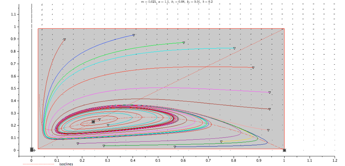
(a) $\lambda<0$ (semi hyperbolic case): $m=0.0025$, $a=1.1$, $k_{1}=0.08$, $k_{2}=0,01$, $b=0.2$.

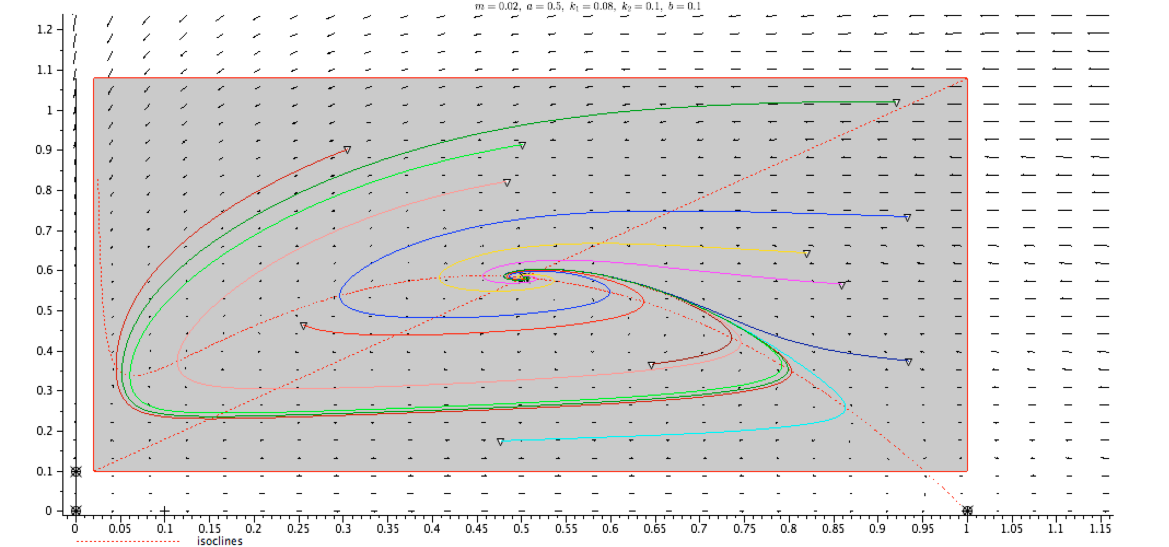
(b) $\lambda>0$ (semi hyperbolic case): $m=0.002$, $a=0.5$, $k_{1}=0.08$, $k_{2}=0.1$, $b=0.1$.

Figure 3: Hopf bifurcation of the system (1.2).

If $\lambda<0$, then the periodic solutions are stable limit cycles, while if $\lambda>0$, the periodic solutions are repelling. See Figure 3 for a numerical exemple.

c- Non-elementary equilibria

Let us rewrite the vector field $\bm{v}=v_{1}\frac{\partial}{\partial x}+v_{2}\frac{\partial}{\partial y}$ associated with (1.2) in the neighborhood of an equilibrium point ${{E}^{*}}=({{x}^{*}},{{y}^{*}})\in\mathcal{A}$. Let ${X}=x-{{x}^{*}}$ and ${Y}=y-{{y}^{*}}$. Since ${{E}^{*}}$ is a critical point of $\bm{v}$, we have

$$v_{1}= \,x(1-x)-\frac{ay(x-m)}{k_{1}+(x-m)}$$

$$= \,({X}+{{x}^{*}})(1-{{x}^{*}}-{X})-\frac{a({Y}+{{y}^{*}})({X}+{{x}^{*}}-m)}{{X}+{{x}^{*}}+k_{1}-m}$$

$$= \,{{x}^{*}}(1-{{x}^{*}})+{X}(1-2{{x}^{*}}-{X})-\frac{a{{y}^{*}}({{x}^{*}}-m)}{{X}+{{x}^{*}}+k_{1}-m}-\frac{a({Y}({X}+{{x}^{*}}-m)+{X}{{y}^{*}})}{{X}+{{x}^{*}}+k_{1}-m}$$

$$= \,{{x}^{*}}(1-{{x}^{*}})-\frac{a{{y}^{*}}({{x}^{*}}-m)}{{{x}^{*}}+k_{1}-m}+{X}(1-2{{x}^{*}}-{X})$$

$$\,+\frac{a{{y}^{*}}({{x}^{*}}-m)}{{{x}^{*}}+k_{1}-m}-\frac{a{{y}^{*}}({{x}^{*}}-m)}{{X}+{{x}^{*}}+k_{1}-m}-\frac{a({Y}({X}+{{x}^{*}}-m)+{X}{{y}^{*}})}{{X}+{{x}^{*}}+k_{1}-m}$$

$$= \,{X}(1-2{{x}^{*}}-{X})+\frac{a{{y}^{*}}({{x}^{*}}-m)}{{{x}^{*}}+k_{1}-m}-\frac{a{{y}^{*}}({{x}^{*}}-m)}{{X}+{{x}^{*}}+k_{1}-m}-\frac{a({Y}({X}+{{x}^{*}}-m)+{X}{{y}^{*}})}{{X}+{{x}^{*}}+k_{1}-m}$$

$$= \,{X}(1-2{{x}^{*}}-{X})+a{{y}^{*}}({{x}^{*}}-m)\left({\frac{1}{{{x}^{*}}+k_{1}-m}-\frac{1}{{X}+{{x}^{*}}+k_{1}-m}}\right)$$

$$\,-\frac{a\Bigl{(}{Y}({X}+{{x}^{*}}-m)+{X}{{y}^{*}}\Bigr{)}}{{X}+{{x}^{*}}+k_{1}-m}$$

$$= \,{X}(1-2{{x}^{*}}-{X})+\frac{a{{y}^{*}}({{x}^{*}}-m){X}}{({{x}^{*}}+k_{1}-m)({X}+{{x}^{*}}+k_{1}-m)}-\frac{a\Bigl{(}{Y}({X}+{{x}^{*}}-m)+{X}{{y}^{*}}\Bigr{)}}{{X}+{{x}^{*}}+k_{1}-m}.$$

For simplification, we denote

(2.36) $$\kappa={{x}^{*}}+k_{1}-m,\quad\rho=\frac{{{x}^{*}}-m}{{{x}^{*}}+k_{1}-m},$$

thus

$$v_{1}={X}(1-2{{x}^{*}}-{X})+\frac{a\Bigl{(}{X}{{y}^{*}}(\rho-1)-{Y}({{x}^{*}}-m)-{Y}{X}\Bigr{)}}{{X}+\kappa}.$$

Using the equality

$$\frac{1}{x+K}=\frac{1}{K}\left({1-\frac{x}{K}+\dots+(-1)^{n}\frac{x^{n}}{K^{n}}+(-1)^{n+1}\frac{x^{n+1}}{K^{n}(x+K)}}\right),\quad n\geq 1,$$

we get

$$v_{1}= \,{X}(1-2{{x}^{*}}-{X})$$

$$\,+\frac{a}{\kappa}\left({1-\frac{{X}}{\kappa}+\frac{{X}^{2}}{\kappa({X}+\kappa)}}\right)\Bigl{(}{X}{{y}^{*}}(\rho-1)-{Y}({{x}^{*}}-m)-{Y}{X}\Bigr{)}$$

$$= \,{X}(1-2{{x}^{*}}-{X})$$

$$\,+\frac{a}{\kappa}\Bigl{(}{X}{{y}^{*}}(\rho-1)-{Y}({{x}^{*}}-m)-{Y}{X}\Bigr{)}$$

$$\,-\frac{a{X}}{\kappa^{2}}\Bigl{(}{X}{{y}^{*}}(\rho-1)-{Y}({{x}^{*}}-m)-{Y}{X}\Bigr{)}$$

$$\,+\frac{a{X}^{2}}{\kappa^{2}({X}+\kappa)}\Bigl{(}{X}{{y}^{*}}(\rho-1)-{Y}({{x}^{*}}-m)-{Y}{X}\Bigr{)}$$

$$= \,{X}\left({1-2{{x}^{*}}+\frac{a}{\kappa}{{y}^{*}}(\rho-1)}\right)-{Y}\frac{a}{\kappa}({{x}^{*}}-m)$$

$$\,-{X}^{2}\left({1+\frac{a}{\kappa^{2}}{{y}^{*}}(\rho-1)}\right)+{X}{Y}\left({-\frac{a}{\kappa}+\frac{a}{\kappa^{2}}({{x}^{*}}-m)}\right)$$

$$\,+\frac{a{X}^{2}{Y}}{\kappa^{2}}+\frac{a{X}^{2}}{\kappa^{2}({X}+\kappa)}\Bigl{(}{X}{{y}^{*}}(\rho-1)-{Y}({{x}^{*}}-m+{X})\Bigr{)}$$

$$= \,{X}\left({1-2{{x}^{*}}-\frac{a{{y}^{*}}k_{1}}{\kappa^{2}}}\right)-{Y}a\rho-{X}^{2}\left({1-\frac{a{{y}^{*}}k_{1}}{\kappa^{3}}}\right)-{X}{Y}\frac{ak_{1}}{\kappa^{2}}$$

$$\,-{X}^{3}\frac{a{{y}^{*}}k_{1}}{\kappa^{3}({X}+\kappa)}+{X}^{2}{Y}\frac{a}{\kappa^{2}}\left({1-\frac{{{x}^{*}}-m+{X}}{{X}+\kappa}}\right)$$

(2.37) $$= \,{X}\left({1-2{{x}^{*}}-\frac{a{{y}^{*}}k_{1}}{\kappa^{2}}}\right)-{Y}a\rho-{X}^{2}\left({1-\frac{a{{y}^{*}}k_{1}}{\kappa^{3}}}\right)-{X}{Y}\frac{ak_{1}}{\kappa^{2}}$$

$$\,-{X}^{3}\frac{a{{y}^{*}}k_{1}}{\kappa^{3}({X}+\kappa)}+{X}^{2}{Y}\frac{ak_{1}}{\kappa^{2}({X}+\kappa)}.$$

Since ${{y}^{*}}={{x}^{*}}+k_{2}-m$, we have also

$$v_{2}= \,b({Y}+{{y}^{*}})\left({1-\frac{{Y}+{{y}^{*}}}{k_{2}+x-m}}\right)=b({Y}+{{y}^{*}})\left({1-\frac{{Y}+{{y}^{*}}}{{X}+{{y}^{*}}}}\right)$$

$$= \,b({X}-{Y})\frac{{Y}+{{y}^{*}}}{{X}+{{y}^{*}}}$$

$$= \,b({X}-{Y})\left({1-({X}-{Y})\frac{1}{{X}+{{y}^{*}}}}\right)$$

(2.38) $$= \,b({X}-{Y})-\frac{b}{{{y}^{*}}}({X}-{Y})^{2}\left({1-\frac{{X}}{{X}+{{y}^{*}}}}\right).$$

This shows in particular that the linear part of $\bm{v}$ is never zero. Thus the only non-hyperbolic cases are the nilpotent case and the case when ${{E}^{*}}$ is a center for the linear part of $\bm{v}$. Let us now investigate these cases:

$\mbox{c}_{1}$. Nilpotent case

This is when $p=0=s$. From the discussion at the beginning of Case b, it is clear that this case is nonempty.

In this case, the Jacobian matrix $\mathcal{J}({{x}^{*}},{{y}^{*}})$ is

$$\mathcal{J}({{x}^{*}},{{y}^{*}})=\begin{pmatrix}b&-b\\ b&-b\end{pmatrix}.$$

With the preceding notations, we thus have

$$v_{1}= \,b({X}-{Y})-{X}^{2}\left({1-\frac{a{{y}^{*}}k_{1}}{\kappa^{3}}}\right)-{X}{Y}\frac{ak_{1}}{\kappa^{2}}-{X}^{3}\frac{a{{y}^{*}}k_{1}}{\kappa^{3}({X}+\kappa)}+{X}^{2}{Y}\frac{ak_{1}}{\kappa^{2}({X}+\kappa)}.$$

The change of variables

$${\mathfrak{u}}={X},\quad{\mathfrak{v}}={Y}-{X}$$

yields

$$v_{1}= \,-{\mathfrak{v}}b-{\mathfrak{u}}^{2}\left({1-\frac{a{{y}^{*}}k_{1}}{\kappa^{3}}}\right)-{\mathfrak{u}}({\mathfrak{u}}+{\mathfrak{v}})\frac{ak_{1}}{\kappa^{2}}-{\mathfrak{u}}^{3}\frac{a{{y}^{*}}k_{1}}{\kappa^{3}({\mathfrak{u}}+\kappa)}+{\mathfrak{u}}^{2}({\mathfrak{u}}+{\mathfrak{v}})\frac{ak_{1}}{\kappa^{2}({\mathfrak{u}}+\kappa)}$$

$$= \,-{\mathfrak{v}}b-{\mathfrak{u}}^{2}\left({1-\frac{a{{y}^{*}}k_{1}}{\kappa^{3}}+\frac{ak_{1}}{\kappa^{2}}}\right)-{\mathfrak{u}}{\mathfrak{v}}\frac{ak_{1}}{\kappa^{2}}$$

$$\,+{\mathfrak{u}}^{3}\frac{ak_{1}}{\kappa^{2}({\mathfrak{u}}+\kappa)}\left({-\frac{{{y}^{*}}}{\kappa}+1}\right)+{\mathfrak{u}}^{2}{\mathfrak{v}}\frac{ak_{1}^{2}}{\kappa^{2}({\mathfrak{u}}+\kappa)},$$

$$v_{2}= \,-{\mathfrak{v}}b-{\mathfrak{v}}^{2}\frac{b}{{{y}^{*}}}\left({1-\frac{{\mathfrak{u}}}{{\mathfrak{u}}+{{y}^{*}}}}\right).$$

The coordinates of $\bm{v}$ are, in the basis $(\frac{\partial}{\partial{\mathfrak{u}}},\frac{\partial}{\partial{\mathfrak{v}}})$,

$$\dot{{\mathfrak{u}}}= \,\dot{{X}}=v_{1},$$

$$\dot{{\mathfrak{v}}}= \,\dot{{Y}}-\dot{{X}}=v_{2}-v_{1}$$

$$= \,-{\mathfrak{v}}b-{\mathfrak{v}}^{2}\frac{b}{{{y}^{*}}}\left({1-\frac{{\mathfrak{u}}}{{\mathfrak{u}}+{{y}^{*}}}}\right)+{\mathfrak{v}}b+{\mathfrak{u}}^{2}\left({1-\frac{a{{y}^{*}}k_{1}}{\kappa^{3}}+\frac{ak_{1}}{\kappa^{2}}}\right)+{\mathfrak{u}}{\mathfrak{v}}\frac{ak_{1}}{\kappa^{2}}$$

$$\,-{\mathfrak{u}}^{3}\frac{ak_{1}}{\kappa^{2}({\mathfrak{u}}+\kappa)}\left({-\frac{{{y}^{*}}}{\kappa}+1}\right)-{\mathfrak{u}}^{2}{\mathfrak{v}}\frac{ak_{1}^{2}}{\kappa^{2}({\mathfrak{u}}+\kappa)}$$

$$= \,{\mathfrak{u}}^{2}\left({1-\frac{a{{y}^{*}}k_{1}}{\kappa^{3}}+\frac{ak_{1}}{\kappa^{2}}}\right)+{\mathfrak{u}}{\mathfrak{v}}\frac{ak_{1}}{\kappa^{2}}-{\mathfrak{v}}^{2}\frac{b}{{{y}^{*}}}+{\mathfrak{u}}^{3}\frac{ak_{1}}{\kappa^{2}({\mathfrak{u}}+\kappa)}\left({\frac{{{y}^{*}}}{\kappa}-1}\right)$$

$$\,-{\mathfrak{u}}^{2}{\mathfrak{v}}\frac{ak_{1}^{2}}{\kappa^{2}({\mathfrak{u}}+\kappa)}+{\mathfrak{u}}{\mathfrak{v}}^{2}\frac{b}{{{y}^{*}}({\mathfrak{u}}+{{y}^{*}})}.$$

We can thus write

(2.39) $$\dot{{\mathfrak{u}}}= \,-{\mathfrak{v}}b+A({\mathfrak{u}},{\mathfrak{v}}),$$

$$\dot{{\mathfrak{v}}}= \,B({\mathfrak{u}},{\mathfrak{v}}),$$

where $A$ and $B$ are analytic and their jacobian matrix at $(0,0)$ is $0$. In the neighborhood of $(0,0)$, the equation $0=-{\mathfrak{v}}b+A({\mathfrak{u}},{\mathfrak{v}})$ has the unique solution ${\mathfrak{v}}={\mathfrak{f}}({\mathfrak{u}})$, where

$${\mathfrak{f}}({\mathfrak{u}})= \frac{-{\mathfrak{u}}^{2}\left({1-\frac{a{{y}^{*}}k_{1}}{\kappa^{3}}+\frac{ak_{1}}{\kappa^{2}}}\right)-{\mathfrak{u}}^{3}\frac{ak_{1}}{\kappa^{2}({\mathfrak{u}}+\kappa)}\left({\frac{{{y}^{*}}}{\kappa}-k_{1}}\right)}{b+{\mathfrak{u}}\frac{ak_{1}}{\kappa^{2}}-{\mathfrak{u}}^{2}\frac{ak_{1}^{2}}{\kappa^{2}({\mathfrak{u}}+\kappa)}}$$

$$= -\frac{1}{b}(1-\frac{a{{y}^{*}}k_{1}}{\kappa^{3}}+\frac{ak_{1}}{\kappa^{2}}){u}^{2}+{\frac{ak1\left(-k1{{y}^{*}}a+{\kappa}^{3}+ak1\kappa+b{\kappa}^{2}-{{y}^{*}}\kappa b\right)}{{b}^{2}{\kappa}^{5}}}{u}^{3}$$

$$+O\left({u}^{4}\right).$$

Let $F({\mathfrak{u}})=B({\mathfrak{u}},{\mathfrak{f}}({\mathfrak{u}}))$. Since $A({\mathfrak{u}},{\mathfrak{f}}({\mathfrak{u}}))=b{\mathfrak{f}}({\mathfrak{u}})$ and $B({\mathfrak{u}},{\mathfrak{v}})$ has the form

$$B({\mathfrak{u}},{\mathfrak{v}})={\mathfrak{v}}b-A({\mathfrak{u}},{\mathfrak{v}})-{\mathfrak{v}}b-{\mathfrak{v}}^{2}\frac{b}{{{y}^{*}}}\left({1-\frac{{\mathfrak{u}}}{{\mathfrak{u}}+{{y}^{*}}}}\right),$$

we have

$$F({\mathfrak{u}})= -b{\mathfrak{f}}({\mathfrak{u}})\,-{\mathfrak{f}}^{2}({\mathfrak{u}})\frac{b}{{{y}^{*}}}\left({1-\frac{{\mathfrak{u}}}{{\mathfrak{u}}+{{y}^{*}}}}\right)$$

$$= {\frac{\left(-k_{1}\,{{y}^{*}}\,a\kappa\,b-{k_{1}}^{2}{{y}^{*}}\,{a}^{2}+{\kappa}^{3}ak_{1}+ak_{1}\,{\kappa}^{2}b+{a}^{2}{{k_{1}}}^{2}\kappa\right){u}^{3}}{{\kappa}^{5}{b}^{2}}}$$

$$+ {\frac{\left(b{\kappa}^{2}k_{1}\,{{y}^{*}}\,a-{\kappa}^{5}b-b{\kappa}^{3}a{k_{1}}\right){u}^{2}}{{\kappa}^{5}{b}^{2}}}+o({\mathfrak{u}}^{3}).$$

Let also $G({\mathfrak{u}})=(\partial A/\partial{\mathfrak{u}}+\partial B/\partial{\mathfrak{v}})({\mathfrak{u}},{\mathfrak{f}}({\mathfrak{u}}))$. We have

$$\partial A/\partial{\mathfrak{u}}= \,-{\mathfrak{v}}\frac{ak_{1}}{\kappa^{2}}-2{\mathfrak{u}}\left({1-\frac{a{{y}^{*}}k_{1}}{\kappa^{3}}+\frac{ak_{1}}{\kappa^{2}}}\right)+2{\mathfrak{u}}{\mathfrak{v}}\frac{ak_{1}}{\kappa^{2}({\mathfrak{u}}+\kappa)}$$

$$\,+3{\mathfrak{u}}^{2}\frac{ak_{1}}{\kappa^{2}({\mathfrak{u}}+\kappa)}\left({-\frac{{{y}^{*}}}{\kappa}+1}\right)-{\mathfrak{u}}^{3}\frac{ak_{1}}{\kappa^{2}({\mathfrak{u}}+\kappa)^{2}}\left({-\frac{{{y}^{*}}}{\kappa}+1}\right)-{\mathfrak{u}}^{2}{\mathfrak{v}}\frac{ak_{1}}{\kappa^{2}({\mathfrak{u}}+\kappa)^{2}},$$

$$\partial B/\partial{\mathfrak{v}}= \,-2{\mathfrak{v}}\frac{b}{{{y}^{*}}}\left({1-\frac{{\mathfrak{u}}}{{\mathfrak{u}}+{{y}^{*}}}}\right)+{\mathfrak{u}}\frac{ak_{1}}{\kappa^{2}}-{\mathfrak{u}}^{2}\frac{ak_{1}}{\kappa^{2}}.$$

Replacing ${\mathfrak{v}}$ by ${\mathfrak{f}}({\mathfrak{u}})$ yields

$$G({\mathfrak{u}})= \,{\mathfrak{u}}\left\lgroup-2\left({1-\frac{a{{y}^{*}}k_{1}}{\kappa^{3}}+\frac{ak_{1}}{\kappa^{2}}}\right)+\frac{ak_{1}}{\kappa^{2}}\right\rgroup$$

$$\,+{\mathfrak{u}}^{2}\left\lgroup\frac{1}{b}\left({1-\frac{a{{y}^{*}}k_{1}}{\kappa^{3}}+\frac{ak_{1}}{\kappa^{2}}}\right)\frac{ak_{1}}{\kappa^{2}}+3\frac{ak_{1}}{\kappa^{3}}\left({-\frac{{{y}^{*}}}{\kappa}+k_{1}}\right)\right\rgroup+o({\mathfrak{u}}^{2}).$$

Case 1: If $1-\frac{a{{y}^{*}}k_{1}}{\kappa^{3}}+\frac{ak_{1}}{\kappa^{2}}\neq 0$, then

$$F({\mathfrak{u}})= u^{2}(1-\frac{a{{y}^{*}}k_{1}}{\kappa^{3}}+\frac{ak_{1}}{\kappa^{2}})+o({\mathfrak{u}}^{2}),$$

and

$$G({\mathfrak{u}})= \,{\mathfrak{u}}\left\lgroup-2\left({1-\frac{a{{y}^{*}}k_{1}}{\kappa^{3}}+\frac{ak_{1}}{\kappa^{2}}}\right)+\frac{ak_{1}}{\kappa^{2}}\right\rgroup$$

$$\,+{\mathfrak{u}}^{2}\left\lgroup\frac{1}{b}\left({1-\frac{a{{y}^{*}}k_{1}}{\kappa^{3}}+\frac{ak_{1}}{\kappa^{2}}}\right)\frac{ak_{1}}{\kappa^{2}}+3\frac{ak_{1}}{\kappa^{3}}\left({-\frac{{{y}^{*}}}{\kappa}+k_{1}}\right)\right\rgroup+o({\mathfrak{u}}^{2}).$$

We can now apply [11, Theorem 3.5] to system (2.39). Since the coefficient of ${\mathfrak{u}}^{2}$ in $F({\mathfrak{u}})$ is nonzero, we deduce from Part (4)-(i1) of [11, Theorem 3.5]:

Lemma 2.9.

If ${{E}^{*}}$ is a nilpotent equilibrium of (1.2) in the positive quadrant $]0,+\infty[\times]0,+\infty[$, and if $1-\frac{a{{y}^{*}}k_{1}}{\kappa^{3}}+\frac{ak_{1}}{\kappa^{2}}\neq 0$, then ${{E}^{*}}$ is a cusp, that is, its phase portrait consists of two hyperbolic sectors and two separatrices. In this case, the index of ${{E}^{*}}$ is 0.

Case 2: if $1-\frac{a{{y}^{*}}k_{1}}{\kappa^{3}}+\frac{ak_{1}}{\kappa^{2}}=0$, then

$${\mathfrak{f}}({\mathfrak{u}})= {\frac{ak1\left(-k1{{y}^{*}}a+{\kappa}^{3}+ak1\kappa+b{\kappa}^{2}-{{y}^{*}}\kappa b\right)}{{b}^{2}{\kappa}^{5}}}{u}^{3}+O\left({u}^{4}\right)$$

$$= -{\frac{1}{b\kappa}}u^{3}+O\left({u}^{3}\right),$$

$$F({\mathfrak{u}})= \frac{1}{\kappa}u^{3}+o({\mathfrak{u}}^{3}),$$

and

$$G({\mathfrak{u}})= {\mathfrak{u}}\left\lgroup\frac{ak_{1}}{\kappa^{2}}\right\rgroup\,+{\mathfrak{u}}^{2}\left\lgroup 3\frac{ak_{1}}{\kappa^{3}}\left({-\frac{{{y}^{*}}}{\kappa}+k_{1}}\right)\right\rgroup+o({\mathfrak{u}}^{2}).$$

Again, we apply [11, Theorem 3.5] to System (2.39). Since the coefficient of ${\mathfrak{u}}^{3}$ in $F({\mathfrak{u}})$ is positive, we deduce from Part (4)-(ii) of [11, Theorem 3.5]:

Lemma 2.10.

If ${{E}^{*}}$ is a nilpotent equilibrium of (1.2) in the positive quadrant $]0,+\infty[\times]0,+\infty[$, and if $1-\frac{a{{y}^{*}}k_{1}}{\kappa^{3}}+\frac{ak_{1}}{\kappa^{2}}=0$, then ${{E}^{*}}$ is a saddle point. In this case, the index of ${{E}^{*}}$ is -1.

$\mbox{c}_{2}$. The case of a center of the linearized vector field

The point ${{E}^{*}}$ is a center of the linear part of $\bm{v}$ if the Jacobian $\mathcal{J}({{x}^{*}},{{y}^{*}})$ has purely imaginary eigenvalues $\pm i\sqrt{p}$, that is, when $p>0$ and $s=0$. Again, this case is nonempty. Let us denote

(2.40) $$b_{0}=1-2{{x}^{*}}+\frac{a{{y}^{*}}k_{1}}{\kappa^{2}}.$$

With the notations of (2.36), we have $p>0$ and $s=0$ if, and only if,

(2.41) $$b=b_{0}<a\rho.$$

Note that ${{x}^{*}}$, ${{y}^{*}}$, as well as $b_{0}$, $a$, $\rho$, and the sign of $p$ do not depend on the parameter $b$, and that $s=b-b_{0}$. Let us fix all parameters except $b$, and assume that $\Delta_{\chi}<0$, that is, the eigenvalues of $\mathcal{J}({{x}^{*}},{{y}^{*}})$ are

$$\frac{-s\pm i\sqrt{4p-s^{2}}}{2}.$$

These eigenvalues cross the imaginary axis at speed $-1/2$ when $b$ passes through the value $b_{0}$. Let us denote $c=a\rho$. By (2.37) and (2.38), we have

$$v_{1}= \,{X}b_{0}-{Y}c-{X}^{2}\left({1-\frac{a{{y}^{*}}k_{1}}{\kappa^{3}}}\right)-{X}{Y}\frac{ak_{1}}{\kappa^{2}}-{X}^{3}\frac{a{{y}^{*}}k_{1}}{\kappa^{3}({X}+\kappa)}+{X}^{2}{Y}\frac{ak_{1}}{\kappa^{2}},$$

$$v_{2}= \,({X}-{Y})b-\frac{b}{{{y}^{*}}}({X}-{Y})^{2}\left({1-\frac{{X}}{{X}+{{y}^{*}}}}\right).$$

Let us denote by $(\bm{i},\bm{j})$ the standard basis of $\mathbb{R}^{2}$. In this basis, the matrix of the linear part $\varphi$ of $({X},{Y})\mapsto(v_{1},v_{2})$ is

$$A(b)=\begin{pmatrix}b_{0}&-c\\ b&-b\end{pmatrix}.$$

Let

$$\delta= \sqrt{\det A(b_{0})}=\sqrt{b_{0}(c-b_{0})}, \gamma=\frac{c-b_{0}}{\delta}=\sqrt{\frac{c-b_{0}}{b_{0}}},$$

$$\bm{u}= \bm{i}+\bm{j}, \bm{v}=\frac{1}{\delta}\varphi(\bm{u})=-\gamma\bm{i}.$$

The matrix of $\varphi$ in the basis $(\bm{u},\bm{v})$ is

$$\tilde{A}(b)=\begin{pmatrix}0&-\frac{b}{b_{0}}\delta\\ \delta&b_{0}-b\end{pmatrix}.$$

The coordinates $({\mathfrak{u}},{\mathfrak{v}})$ in the basis $(\bm{u},\bm{v})$ satisfy ${\mathfrak{u}}={Y},\quad{\mathfrak{v}}=\frac{1}{\gamma}({Y}-{X})$, ${X}={\mathfrak{u}}-{\mathfrak{v}}\gamma$, ${Y}={\mathfrak{u}}$. The coordinates of $\bm{v}$ in the basis $(\frac{\partial}{\partial{\mathfrak{u}}},\frac{\partial}{\partial{\mathfrak{v}}})$ are

$$\dot{{\mathfrak{u}}} \,=v_{2}=-b\gamma{\mathfrak{v}}+\frac{b}{{{y}^{*}}}\gamma^{2}{\mathfrak{v}}^{2}\left({1-\frac{{\mathfrak{u}}-{\mathfrak{v}}\gamma}{{\mathfrak{u}}-{\mathfrak{v}}\gamma+{{y}^{*}}}}\right),$$

$$\dot{{\mathfrak{v}}}= \,\frac{1}{\gamma}(v_{2}-v_{1})$$

$$= \,-b{\mathfrak{v}}+\frac{b}{{{y}^{*}}}\gamma{\mathfrak{v}}^{2}\left({1-\frac{{\mathfrak{u}}-{\mathfrak{v}}\gamma}{{\mathfrak{u}}-{\mathfrak{v}}\gamma+{{y}^{*}}}}\right)$$

$$\,-\frac{1}{\gamma}\Biggl{\lgroup}({\mathfrak{u}}-{\mathfrak{v}}\gamma)b_{0}-{\mathfrak{u}}c-({\mathfrak{u}}-{\mathfrak{v}}\gamma)^{2}\left({1-\frac{a{{y}^{*}}k_{1}}{\kappa^{3}}}\right)-{\mathfrak{u}}({\mathfrak{u}}-{\mathfrak{v}}\gamma)\frac{ak_{1}}{\kappa^{2}}$$

$$\,\phantom{-\frac{1}{\gamma}\Biggl{\lgroup}}-({\mathfrak{u}}-{\mathfrak{v}}\gamma)^{3}\frac{a{{y}^{*}}k_{1}}{\kappa^{3}({\mathfrak{u}}-{\mathfrak{v}}\gamma+\kappa)}+{\mathfrak{u}}({\mathfrak{u}}-{\mathfrak{v}}\gamma)^{2}\frac{ak_{1}}{\kappa^{2}}\Biggr{\rgroup}.$$

In particular, for $$b=b_{0}$$,

$$\dot{{\mathfrak{u}}}= \,-\delta{\mathfrak{v}}+\frac{c-b_{0}}{{{y}^{*}}}{\mathfrak{v}}^{2}\left({1-\frac{{\mathfrak{u}}-{\mathfrak{v}}\gamma}{{\mathfrak{u}}-{\mathfrak{v}}\gamma+{{y}^{*}}}}\right),$$

$$\dot{{\mathfrak{v}}}= \,\delta{\mathfrak{u}}+\frac{c-b_{0}}{{{y}^{*}}}{\mathfrak{v}}^{2}\left({1-\frac{{\mathfrak{u}}-{\mathfrak{v}}\gamma}{{\mathfrak{u}}-{\mathfrak{v}}\gamma+{{y}^{*}}}}\right)$$

$$\,+\frac{1}{\gamma}\Biggl{\lgroup}+({\mathfrak{u}}-{\mathfrak{v}}\gamma)^{2}\left({1-\frac{a{{y}^{*}}k_{1}}{\kappa^{3}}}\right)+{\mathfrak{u}}({\mathfrak{u}}-{\mathfrak{v}}\gamma)\frac{ak_{1}}{\kappa^{2}}$$

$$\,\phantom{-\frac{1}{\gamma}\Biggl{\lgroup}}+({\mathfrak{u}}-{\mathfrak{v}}\gamma)^{3}\frac{a{{y}^{*}}k_{1}}{\kappa^{3}({\mathfrak{u}}-{\mathfrak{v}}\gamma+\kappa)}-{\mathfrak{u}}({\mathfrak{u}}-{\mathfrak{v}}\gamma)^{2}\frac{ak_{1}}{\kappa^{2}}\Biggr{\rgroup}.$$

2.3 Existence of a globally asymptotically stable equilibrium point

When $m=0$, in the case (c) of Theorem 2.4, we have seen that (1.2) has no cycle, because the compact set delimited by a cycle would contain a critical point, see [5, Theorem V.3.8]. As the compact set $\mathcal{A}$ is invariant and contains all equilibrium points of the open quadrant $]0,+\infty[\times]0,+\infty[$, all trajectories starting in the quadrant $\mathbb{R}_{+}\times\mathbb{R}_{+}$ converge to $E_{1}$ or $E_{2}$ ($E_{0}$ is excluded because it is an unstable node). On the $x$ axis, we have $\dot{y}=0$ and $x$ satisfies the logistic equation $\dot{x}=x(1-x)$, thus, for $x(0)>0$, $x(t)$ converges to 1, i.e., $(x(t),y(t))$ converges to $E_{1}$. On the other hand, for $0<y<k_{2}+x$, we have $\dot{y}>0$, thus, if $y(0)>0$, $(x(t),y(t))$ cannot converge to $E_{1}$, it converges necessarily to $E_{2}$.

Theorem 2.11.

A sufficient condition for the existence of a globally asymptotically stable equilibrium point ${{E}^{*}}=({{x}^{*}},{{y}^{*}})$ in the open quadrant $]0,+\infty[\times]0,+\infty[$ (equivalently, in the interior of $\mathcal{A}$) is that

(2.42) $$\big{\lgroup}2m+k_{1}\geq 1\big{\rgroup}\text{ and }\big{\lgroup}(m>0)\text{ or }\bigl{(}4ak_{2}\leq(1-k_{1}-a)^{2}+4k_{1}\bigr{)}\big{\rgroup}.$$

Proof.

Let ${{E}^{*}}=({{x}^{*}},{{y}^{*}})\in\mathcal{A}$ be an equilibrium point in the interior of $\mathcal{A}$. Let us denote

$$\rho(x)=\frac{a(x-m)}{k_{1}+x-m},$$

and let us set

$$V(x,y)=\int_{{x}^{*}}^{x}\frac{u-{{x}^{*}}}{(k_{2}+u-m)\rho(u)}\,\mathrm{d}u+\frac{1}{b}\int_{{y}^{*}}^{y}\frac{v-{{y}^{*}}}{v}\,\mathrm{d}v.$$

Then, using (2.20) and (2.21), we have

$$\dot{V}= \,\frac{x-{{x}^{*}}}{(k_{2}+x-m)\rho(x)}\,\dot{x}+\frac{1}{b}\frac{y-{{y}^{*}}}{y}\,\dot{y}$$

$$= \,\frac{x-{{x}^{*}}}{k_{2}+x-m}\left({\frac{x(1-x)}{\rho(x)}-\frac{a(x-m)}{k_{1}+x-m}\frac{1}{\rho(x)}y}\right)+\frac{1}{b}(y-{{y}^{*}})b\left({1-\frac{y}{k_{2}+x-m}}\right)$$

$$= \,\frac{x-{{x}^{*}}}{a(k_{2}+x-m)}\left({\frac{x(1-x)(k_{1}+x-m)}{x-m}-{{y}^{*}}}\right)-\frac{(x-{{x}^{*}})(y-{{y}^{*}})}{k_{2}+x-m}$$

$$\,+(y-{{y}^{*}})\left({\frac{{{y}^{*}}}{k_{2}+{{x}^{*}}-m}-\frac{y}{k_{2}+x-m}}\right)$$

$$= \,\frac{x-{{x}^{*}}}{a(k_{2}+x-m)}\left({\frac{x(1-x)(k_{1}+x-m)}{x-m}-\frac{{{x}^{*}}(1-{{x}^{*}})(k_{1}+{{x}^{*}}-m)}{{{x}^{*}}-m}}\right)$$

$$\,-\frac{(x-{{x}^{*}})(y-{{y}^{*}})}{k_{2}+x-m}$$

$$\,+(y-{{y}^{*}})\,{\frac{{{y}^{*}}(k_{2}+x-m)-y(k_{2}+{{x}^{*}}-m)}{(k_{2}+{{x}^{*}}-m)(k_{2}+x-m)}}.$$

Let us denote $${\mathfrak{g}}(x)=x(1-x)(k_{1}+x-m)/(x-m)$$. Then

$$\dot{V}= \,\frac{x-{{x}^{*}}}{a(k_{2}+x-m)}\left({{\mathfrak{g}}(x)-{\mathfrak{g}}({{x}^{*}})}\right)-\frac{(x-{{x}^{*}})(y-{{y}^{*}})}{k_{2}+x-m}$$

$$\,+(y-{{y}^{*}})\,\frac{({{y}^{*}}-y)(k_{2}-m)+{{y}^{*}}x-y{{x}^{*}}}{(k_{2}+{{x}^{*}}-m)(k_{2}+x-m)}$$

$$= \,\frac{x-{{x}^{*}}}{a(k_{2}+x-m)}\left({{\mathfrak{g}}(x)-{\mathfrak{g}}({{x}^{*}})}\right)-\frac{(x-{{x}^{*}})(y-{{y}^{*}})}{k_{2}+x-m}$$

$$\,+\frac{y-{{y}^{*}}}{{{y}^{*}}}\,\frac{({{y}^{*}}-y)({{x}^{*}}+k_{2}-m)+{{y}^{*}}(x-{{x}^{*}})}{k_{2}+x-m}$$

$$= \,\frac{x-{{x}^{*}}}{a(k_{2}+x-m)}\left({{\mathfrak{g}}(x)-{\mathfrak{g}}({{x}^{*}})}\right)+\frac{y-{{y}^{*}}}{{{y}^{*}}}\,\frac{({{y}^{*}}-y)({{x}^{*}}+k_{2}-m)}{k_{2}+x-m}$$

$$= \,\frac{1}{k_{2}+x-m}\left({\frac{x-{{x}^{*}}}{a}\left({{\mathfrak{g}}(x)-{\mathfrak{g}}({{x}^{*}})}\right)-(y-{{y}^{*}})^{2}}\right).$$

For $x\geq m$, a sufficient condition for $\dot{V}$ to be negative when $(x,y)\not=({{x}^{*}},{{y}^{*}})$ is that ${\mathfrak{g}}$ be nonincreasing. Let us make the change of variable $X=x-m$. We have

$${\mathfrak{g}}(x)=\frac{(X+m)(1-X-m)(X+k_{1})}{X},$$

which leads to

$${\mathfrak{g}}^{\prime}(x)=\frac{-2X^{3}+(1-2m-k_{1})X^{2}-k_{1}(m-m^{2})}{X^{2}}.$$

Thus, if $2m+k_{1}\geq 1$, ${\mathfrak{g}}^{\prime}(X)$ remains negative for $X>0$, i.e., for $x>m$. Thus, for $x>m$, under the assumption (2.42), $\dot{V}$ is negative.

We have seen that the first part of (2.42) implies that the equilibrium point ${{E}^{*}}$, if it exists, is globally asymptotically stable. Note that Condition (2.42) is independent of the coordinates of ${{E}^{*}}$, and the global stability implies that the equilibrium point ${{E}^{*}}$, if it exists, is unique.

The second part of (2.42) is a necessary and sufficient condition for the existence of such an equilibrium point.

When $m>0$, we already know that there exists at least one equilibrium point in $\mathcal{A}$. Actually, Condition (2.42) implies that the coefficient $\alpha_{2}=a+k_{1}-1+2m$ of (2.23) is positive. Thus, when $m>0$, (2.42) is a particular case of (c) in Theorem 2.3.

When $m=0$, by Theorem 2.4-(c), since $\alpha_{2}>0$, there exists an equilibrium point in the interior of $\mathcal{A}$ if, and only if, (2.29) is satisfied. ∎

2.4 Cycles

Let us investigate the existence of periodic orbits of (1.2). By Theorem 2.1 such orbits can take place only in $\mathcal{A}$.

2.4.1 Refuge free case ($m=0$)

This case has been studied by M.A. Aziz-Alaoui and M. Daher-Okiye [9], but we add some new results.

Lemma 2.12.

In the cases (c) and (a) of Theorem 2.4, that is, when (1.2) has 0 or 2 equilibrium points in the open quadrant $]0,+\infty[\times]0,+\infty[$, the system (1.2) has no limit cycle. On the other hand, in the case (b) of Theorem theorem 2.4, that is, when (1.2) has 1 equilibrium point in the open quadrant $]0,+\infty[\times]0,+\infty[$, if furthermore $s<0$ and $p>0$, the system (1.2) has at least one limit cycle.

Proof.

In the case (c), the only equilibrium points of (1.2) in $\mathbb{R}_{+}\times\mathbb{R}_{+}$ are the trivial points $E_{0}$, $E_{1}$, and $E_{2}$, on the axes. Thus (1.2) has no cycle, because the compact set delimited by a cycle would contain a critical point, see [5, Theorem V.3.8].

In the case (a), if there was a cycle inside $\mathcal{A}$, we could apply the Poincaré-Hopf Index Theorem to the compact manifold whose boundary is delineated by this cycle (see [26] for a version of this theorem when the vector field is tangent to the boundary). Denoting $N$ the number of nodes or foci and $S$ the number of saddles in the open quadrant $]0,+\infty[\times]0,+\infty[$, we would have $N-S=1$. But Theorem 2.5 shows that $N-S=0$, a contradiction.

In the case (b), if $s<0$ and $p>0$, the system (1.2) has an unstable equilibrium point. From Theorem 2.1 and Poincaré-Bendixson Theorem, there exists at least one limit cycle around this equilibrium. ∎

Note that the conditions of Lemma 2.12 do not involve the value of $b$. Using Bendixson-Dulac criterion, M.A. Aziz-Alaoui and M. Daher-Okiye obtain another criterion:

Lemma 2.13.

[9, Theorem 7] if $b+k_{1}\geq 1$, then the system (1.2) has no limit cycle.

2.4.2 Case with refuge ($m>0$)

By Theorem 2.11, if Condition (2.42) is satisfied, there can be no periodic orbits.

Let us now give some sufficient conditions for the absence of periodic orbits, using Bendixson-Dulac criterion. Let us denote by $v_{1}(x,y)$ and $v_{2}(x,y)$ the coordinates of the vector field in (1.2). For a Dulac function, we choose

$$D(x,y)=x+k_{1}-m.$$

Let us look for conditions that ensure that $\frac{\partial(v_{1}D)}{\partial x}+\frac{\partial(v_{2}D)}{\partial y}<0$ in $\mathcal{A}$. We have

$$\frac{\partial(v_{1}D)}{\partial x}(x,y) =-3x^{2}+2(1-k_{1}+m)x+k_{1}-m-ay,$$

$$\frac{\partial(v_{2}D)}{\partial y}(x,y) =\frac{b(x+k_{1}-m)(x+k_{2}-m-2y)}{x+k_{2}-m}.$$

For $(x,y)\in\mathcal{A}$, we have

$$\frac{\partial(v_{1}D)}{\partial x}(x,y)<-3m^{2}+2(1-k_{1}+m)x+k_{1}-m-ak_{2}.$$

Since the maximum of $-3m^{2}+m$ is $1/12$ and the maximum of $-m^{2}+m$ is $1/4$, we deduce:

$$1-k_{1}+m>0\Rightarrow\frac{\partial(v_{1}D)}{\partial x}(x,y) <-3m^{2}+m-k_{1}-ak_{2}+2$$

$$\leq 2+\frac{1}{12}-k_{1}-ak_{2},$$

$$1-k_{1}+m<0\Rightarrow\frac{\partial(v_{1}D)}{\partial x}(x,y) <-m^{2}+m(1-2k_{1})-k_{1}-ak_{2}$$

$$<-m^{2}-m-k_{1}-ak_{2}<0.$$

In particular, a condition that ensures that $\frac{\partial(v_{1}D)}{\partial x}<0$ in $\mathcal{A}$ is

(2.43) $$(k_{1}>1+m)\text{ or }(ak_{2}+k_{1}>2+\frac{1}{12}).$$

On the other hand, for $(x,y)\in\mathcal{A}$, $\frac{\partial(v_{2}D)}{\partial y}(x,y)$ has the same sign as $x+k_{2}-m-2y$, and we have $x+k_{2}-m-2y<1-m-k_{2}$. Thus a sufficient condition for $\frac{\partial(v_{2}D)}{\partial x}<0$ in $\mathcal{A}$ is

(2.44) $$k_{2}>1-m.$$

The same technique does not provide any sufficient condition for $\frac{\partial(v_{1}D)}{\partial x}+\frac{\partial(v_{2}D)}{\partial y}>0$ in $\mathcal{A}$. So, our next result concerning the absence of cycles is:

Lemma 2.14.

A sufficient condition for (1.2) to have no periodic solution is

$$\big{\lgroup}k_{2}>1-m\big{\rgroup}\text{ and }\big{\lgroup}(k_{1}>1+m)\text{ or }(ak_{2}+k_{1}>2+\frac{1}{12})\big{\rgroup}.$$

Now, we consider the existence of limit cycles which are not occuring from a Hopf bifurcation. The special configuration of the existence of a limit cycle enclosing three equilibrium points is numerically investigated. In particular, when the system parameters satisfy $a=0.5,k1=0.08,k2=0.2,b=0.1,m=0.0025,$ then three hyperbolic equilibrium points exist, namely, $E_{1}^{*}=(0.0222589;0.2197589)$, $E_{2}^{*}=(0.0299525;0.2274525)$, $E_{3}^{*}=(0.3702886;0.5677886)$. They define respectively a stable focus, a saddle point and an unstable focus. Accordingly to the Poincaré index theorem, the sum of the corresponding indexes is equal to $1$.

The numerical simulations show that there exists a limit cycle, which is hyperbolic and stable, see Figure 1.

3 Stochastic model

We now study the dynamics of the system (1.3), with initial conditions $x_{0}>0$ and $y_{0}>0$. In the case when $m=0$ and $k_{1}=k_{2}$, the persistence and boundedness of solutions have been investigated in by Ji, Jiang and Shi in [17]. A similar model has been studied by Fu, Jiang, Shi, Hayat and Alsaedi in [13].

3.1 Existence and uniqueness of the positive global solution

Theorem 3.1.

For any initial condition $(x_{0},y_{0})\in\mathbb{R}_{+}^{2}$, the system (1.3) admits a unique solution $(x(t),y(t))$, defined for all $t\geq 0$ a.s. and this solution remains in $]0,+\infty[\times]0,+\infty[$. Furthermore, if $(x_{0},y_{0})\in]0,+\infty[\times]0,+\infty[$, this solution remains in $]0,+\infty[\times]0,+\infty[$, whereas, if $(x_{0},y_{0})$ belongs to one of the axis $\mathbb{R}_{+}\times\{0\}$ or $\{0\}\times\mathbb{R}_{+}$, it remains on this axis.

Proof.

Since the coefficients of (1.3) are locally Lipschitz, uniqueness of the solution until explosion time is guaranteed for any initial condition.

Let us now prove global existence of the solution.

The case when $(x_{0},y_{0})\in\Bigl{(}\mathbb{R}_{+}\times\{0\}\Bigr{)}\cup\Bigl{(}\{0\}\times\mathbb{R}_{+}\Bigr{)}$ is trivial because both equations in (1.3) become independent, for example if $y_{0}=0$ with $x_{0}\not=0$, we have $y(t)=0$ for all $t\geq 0$, and $x$ is a solution to the stochastic logistic equation

$$dx(t)=x(t)(1-x(t))dt+\sigma_{1}x(t)dw_{1}(t)$$

which is well known (see Section 3.2), thus $x(t)$ is defined for every $t\geq 0$.

Assume now that $x_{0}>0$ and $y_{0}>0$. Since the coordinate axes are stable by (1.3), we deduce, applying locally the comparaison theorem for SDEs (see [12, Theorem 1], this theorem is given for globally Lipschitz coefficients), that the solution to (1.3) remains in $]0,+\infty[\times]0,+\infty[$ until its explosion time.

Let $\tau_{e}$ be the explosion time of the solution to (1.3). To show that $\tau_{e}=\infty$, we adapt the proof of [10]. Let $k_{0}>0$ be large enough, such that $\left(x_{0},y_{0}\right)\in[\frac{1}{k_{0}},k_{0}]\times[\frac{1}{k_{0}},k_{0}]$. For each integer $k\geq k_{0}$ we define the stopping time

$$\tau_{k}=\inf\Big{\{}t\in[0,\tau_{e}):x\notin(\frac{1}{k},k)\text{\ or \ }y\notin(\frac{1}{k},k)\Big{\}}.$$

The sequence $(\tau_{k})$ is increasing as $k\rightarrow\infty$. Set $\tau_{\infty}=\lim_{k\rightarrow\infty}\tau_{k}$, whence $\tau_{\infty}\leq\tau_{e}$, (in fact, as $(x(t),y(t))>0$ a.s., we have $\tau_{\infty}=\tau_{e}$). It suffices to prove that $\tau_{\infty}=\infty$ a.s.. Assume that this statement is false, then there exist $T>0$ and $\varepsilon\in\left]0,1\right[$ such that $\operatorname{\mathrm{P}}\left(\{\tau_{\infty}\leq T\}\right)>\varepsilon$. Since $(\tau_{k})$ is increasing we have

$$\operatorname{\mathrm{P}}\left(\{\tau_{k}\leq T\}\right)>\varepsilon.$$

Consider now the positive definite function $V$ : $]0,+\infty[\times]0,+\infty[\rightarrow]0,+\infty[\times]0,+\infty[$ given by

$$V(x,y)=(x+1-\log x)+(y+1-\log y).$$

Applying Itô’s formula, we get

$$dV(x,y)= \Big{[}(x-1)(1-x-\frac{ay(x-m)}{k_{1}+x-m})+\frac{\sigma_{1}^{2}}{2}+b(y-1)(1-\frac{y}{k_{2}+x-m})+\frac{\sigma_{2}^{2}}{2}\Big{]}dt$$

$$+ \sigma_{1}(x-1)dW_{1}+\sigma_{2}(y-1)dW_{2}.$$

The positivity of $x(t)$ and $y(t)$ implies

$$dV(x,y) \leq\Big{(}2x+ay+\frac{\sigma_{1}^{2}+\sigma_{2}^{2}}{2}+by+\frac{y}{k_{2}}\Big{)}dt+\sigma_{1}(x-1)dW_{1}+\sigma_{2}(y-1)dW_{2}$$

$$\leq\Big{(}2x+(a+b+\frac{1}{k_{2}})y+\frac{\sigma_{1}^{2}+\sigma_{2}^{2}}{2}\Big{)}dt+\sigma_{1}(x-1)dW_{1}+\sigma_{2}(y-1)dW_{2}.$$

Denote $c_{1}=a+b+\frac{1}{k_{2}}$, $c_{2}=\frac{\sigma_{1}^{2}+\sigma_{2}^{2}}{2}$. Using [10, lemma 4.1], we can write

$$2x+c_{1}y\leq 4(x+1-\log x)+2c_{1}(y+1-\log y)$$

$$\leq c_{3}V(x,y),$$

where $c_{3}=\max(4,2c_{1})$. Hence, denoting $c_{4}=\max(c_{2},c_{3})$,

$$dV(x,y)\leq (c_{2}+c_{3}V(x,y))dt+\sigma_{1}(x-1)dW_{1}+\sigma_{2}(y-1)dW_{2}$$

$$\leq c_{4}(1+V(x,y))dt+\sigma_{1}(x-1)dW_{1}+\sigma_{2}(y-1)dW_{2}.$$

Integrating both sides from $0$ to $\tau_{k}\wedge T$, and taking expectations, we get

$$\operatorname{\mathrm{E}}V(x(\tau_{k}\wedge T),y(\tau_{k}\wedge T))\leq V(x_{0},y_{0})+c_{4}T+c_{4}\int_{0}^{T}\operatorname{\mathrm{E}}V(x(\tau_{k}\wedge t),y(\tau_{k}\wedge t)dt.$$

By Gronwall’s inequality, this yields

(3.1) $$\operatorname{\mathrm{E}}V(x(\tau_{k}\wedge T),y(\tau_{k}\wedge T))\leq c_{5},$$

where $c_{5}$ is the finite constant given by

(3.2) $$c_{5}=(V(x_{0},y_{0})+c_{4}T)e^{c_{4}T}.$$

Let $\Omega_{k}=\{\tau_{k}\leq T\}$. We have $\operatorname{\mathrm{P}}(\Omega_{k})\geq\varepsilon$, and for all $\omega\in\Omega_{k}$, there exists at least one element of ${x(\tau_{k},\omega),y(\tau_{k},\omega)}$ which is equal either to $k$ or to $\frac{1}{k}$, hence

$$V(x(\tau_{k}),y(\tau_{k}))\geq(k+1-\log k)\wedge(\frac{1}{k}+1+\log k).$$

Therefore, by (3.1),

$$c_{5}\geq\operatorname{\mathrm{E}}[1_{\Omega_{k}}(\omega)V(x(\tau_{k},\omega),y(\tau_{k},\omega)]\geq\varepsilon\Big{[}(k+1-\log k)\wedge(\frac{1}{k}+1+\log k)\Big{]},$$

where $1_{\Omega_{k}}$ is the indicator function of $\Omega_{k},$. Letting $k\rightarrow\infty$, we get $c_{5}=\infty$, which contradicts (3.2), So we must have $\tau_{\infty}=\infty$ a.s. ∎

Remark 8.

An alternative proof of non explosion in finite time can be obtained by using the comparison theorem, since $0\leq x(t)\leq z_{1}(t)$ and $0\leq y(t)\leq z_{2}(t)$ a.s. for every $t\geq 0$, where $z_{1}$ and $z_{2}$ are geometric Brownian motions, with

$$dz_{1}(t)=z_{1}(t)dt+\sigma_{1}z_{1}(t)dW_{1}(t)\text{ and }dz_{2}(t)=bz_{2}(t)dt+\sigma_{2}z_{2}(t)dW_{2}(t).$$

3.2 Comparison results

In this section, we compare the dynamics of (1.3) with some simpler models, in view of applications to the long time behaviour of the solutions to (1.3).

Applying locally the comparaison theorem for SDEs (see [12, Theorem 1], this theorem is given for globally Lipschitz coefficients), we have, for every $t\geq 0$,

(3.3) $$0\leq x(t)\leq u(t)\text{ a.s.}$$

where $u$ is the solution to the stochastic logistic equation (also called stochastic Verhulst equation) with initial condition $x_{0}$:

(3.4) $$du(t)=u(t)(1-u(t))dt+\sigma_{1}u(t)dw_{1}(t),\quad u(0)=x_{0}.$$

The process $u$ is well known and can be written explicitely, see [19, page 125]:

$$u(t)=\frac{e^{\bigl{(}1-\frac{\sigma_{1}^{2}}{2}\bigr{)}t+\sigma_{1}w_{1}(t)}}{\frac{1}{x_{0}}+\int_{0}^{t}e^{\bigl{(}1-\frac{\sigma_{1}^{2}}{2}\bigr{)}s+\sigma_{1}w_{1}(s)}ds}.$$

By [21, Lemma 2.2], $u$ is uniformly bounded in $L^{p}$ for every $p>0$. Thus, by (3.3), for every $p>0$, there exists a constant $K_{p}$ such that

(3.5) $$\sup_{t\geq 0}\operatorname{\mathrm{E}}\left(x(t)\right)^{p}<K_{p}.$$

Using again the comparison theorem, we get, for every $t\geq 0$,

(3.6) $$0\leq y(t)\leq v(t),$$

where $v$ is the solution to

(3.7) $$dv(t)=bv(t)\left({1-\frac{v(t)}{k_{2}+u(t)}}\right)dt+\sigma_{2}v(t)dw_{2}(t),\quad v(0)=y_{0},$$

which can be explicited with the help of $u$:

(3.8) $$v(t)=\frac{e^{\bigl{(}b-\frac{\sigma_{2}^{2}}{2}\bigr{)}t+\sigma_{2}w_{2}(t)}}{\frac{1}{y_{0}}+b\int_{0}^{t}\frac{1}{k_{2}+u(s)}e^{\bigl{(}b-\frac{\sigma_{2}^{2}}{2}\bigr{)}s+\sigma_{2}w_{2}(s)}ds}.$$

Similarly, we have, for every $t\geq 0$,

(3.9) $$0 \leq\check{u}(t)\leq x(t)\text{ a.s.},$$

(3.10) $$0 \leq\check{v}(t)\leq y(t)\text{ a.s.},$$

with

(3.11) $$d\check{u}(t) =\Bigl{(}\check{u}(t)(1-\check{u}(t))-av(t)\Bigr{)}dt+\sigma_{1}\check{u}(t)dw_{1}(t),\quad\check{u}(0)=x_{0},$$

(3.12) $$d\check{v}(t) =b\check{v}(t)\left({1-\frac{\check{v}(t)}{k_{2}}}\right)dt+\sigma_{2}\check{v}(t)dw_{2}(t),\quad\check{v}(0)=y_{0}.$$

Note that $\check{u}$ is defined with the help of the process $v$ defined by (3.7).

The following property of stochastic logistic processes will be useful:

Lemma 3.2.

([21, Theorem 3.2 and Theorem 4.1]) The process $u$ converges a.s. to $0$ if $\sigma_{1}^{2}\geq 2$, whereas it converges to a nondegenerate stationary distribution if $0<\sigma_{1}^{2}<2$.

Similarly, $\check{v}$ converges a.s. to $0$ if $\sigma_{2}^{2}\geq 2b$, whereas it converges to a nondegenerate stationary distribution if $0<\sigma_{2}^{2}<2$.

Remark 9.

The global existence and uniqueness of $(u,v,\check{u},\check{v})$ can be obtained via the same methods as in Section 3.1, see in particular Remark 8.

3.3 Extinction

We show that, when the noise is large, the system (1.3) goes almost surely (but in infinite time) to extinction.

Theorem 3.3.

Assume that $\sigma_{1}^{2}\geq 2$. Then $\lim_{t\rightarrow\infty}x(t)=0$ a.s. If moreover $\sigma_{2}^{2}\geq 2b$, then $\lim_{t\rightarrow\infty}y(t)=0$ a.s.

Proof.

If $\sigma_{1}^{2}\geq 2$, we deduce from (3.4) and Lemma 3.2 that $x(t)$ converges to $0$ a.s.

Assume moreover that $\sigma_{2}^{2}\geq 2b$. From (3.8), the random variable $v:\,\Omega\rightarrow C(\mathbb{R}_{+};\mathbb{R}_{+})$ is a function of two independent random variables, $w_{2}$ and $u$ (the latter is a function of $w_{1}$). For a fixed $u\in C(\mathbb{R}_{+};\mathbb{R}_{+})$ such that $\lim_{t\rightarrow\infty}u(t)=0$, we have

(3.13) $$\lim_{t\rightarrow\infty}\bigl{(}v(t)-\check{v}(t)\bigr{)}=0,$$

where $\check{v}$ is defined by (3.11). Thus, since $u(t)$ goes to $0$ a.s., Equation 3.13 is satisfied a.s. Since, by Lemma 3.2, $\check{v}(t)$ converges a.s. to $0$ if $\sigma_{2}^{2}\geq 2b$, we deduce that $\lim_{t\rightarrow\infty}v(t)=0$ a.s., and the result follows from (3.6). ∎

Remark 10.

Since $\check{v}(t)\leq y(t)\leq v(t)$, we can deduce also from (3.13) that, if $\sigma_{1}^{2}\geq 2$ with $0<\sigma_{2}^{2}<2b$, then $x(t)$ converges a.s. to $0$ while $y(t)$ converges to a nondegenerate stationary distribution.

3.4 Existence of a stationary distribution

In this section, we assume that $m>0$. The existence of a stationary distribution is proved for a similar (but different) system without refuge in [13].

Theorem 3.4.

Assume that $0<\sigma_{1}^{2}<2$ and $0<\sigma_{2}^{2}<2b$, with $m>0$. Then the system (1.3) has a unique stationary distribution $\mu$ on $]0,+\infty[\times]0,+\infty[$. Moreover, the system (1.3) is ergodic and its transition probility $\operatorname{\mathrm{P}}((x,y),t,.)$ satisfies

$$\operatorname{\mathrm{P}}((x_{0},y_{0}),t,\varphi)\rightarrow\mu(\varphi)\text{ when }t\rightarrow\infty$$

for each $(x_{0},y_{0})\in]0,+\infty[\times]0,+\infty[$ and each bounded continuous function $\varphi:\,\allowbreak]0,+\infty[\times]0,+\infty[\allowbreak\rightarrow\allowbreak\mathbb{R}$.

Remark 11.

Theorem 3.4 shows that, contrarily to the deterministic case, when $\min\{\sigma_{1},\sigma_{2}\}>0$, there is only one equilibrium for the system (1.3) in the open quadrant $]0,+\infty[\times]0,+\infty[$.

Note also that, when $\min\{\sigma_{1},\sigma_{2}\}>0$, there is no invariant closed subset in the open quadrant $]0,+\infty[\times]0,+\infty[$ for the system (1.3). Indeed, since the noise in (1.3) acts in all directions, the viability conditions of [8] are satisfied for no closed convex subset of $]0,+\infty[\times]0,+\infty[$.

In particular, there is no equilibrium point for (1.3), thus the limit stationary distribution is nondegenerate.

Remark 12.

The ecologically less interesting case when $(x,y)$ stays in one of the coordinate axes has similar features, since, by [21, Theorem 3.2], the stochastic logistic equation admits a unique invariant ergodic distribution when the diffusion coefficient is positive but not too large.

Our proof of Theorem 3.4 is based on the following well known result:

Lemma 3.5.

Consider the equation

(3.14) $$dX(t)=f(X(t))\,dt+g(X(t))\,dW(t)$$

where $f:\,\mathbb{R}^{d}\rightarrow\mathbb{R}^{d}$ and $g:\,\mathbb{R}^{d}\rightarrow\mathbb{R}^{m\times d}$ are locally Lipschitz functions with locally sublinear growth, and $W$ is a standard Brownian motion on $\mathbb{R}^{m}$. Denote by $A(x)$ the $m\times m$ matrix $g(x)\,g(x)^{T}$. Assume that $]0,+\infty[^{d}$ is invariant by (3.14) and that there exists a bounded open subset $U$ of $]0,+\infty[^{d}$ such that the following conditions are satisfied:

• In a neighborhood of $U$, the smallest eigenvalue of $A(x)$ is bounded away from $0$,

• If $x\in\mathbb{R}^{d}\setminus U$, the expectation of the hitting time $\tau^{U}$ at which the solution to (3.14) starting from $x$ reaches the set $U$ is finite, and $\sup_{x\in K}\operatorname{\mathrm{E}}^{x}\tau^{U}<\infty$ for every compact subset $K$ of $]0,+\infty[^{d}$.

Then (3.14) has a unique stationary distribution $\mu$ on $]0,+\infty[^{d}$. Moreover, (3.14) is ergodic, its transition probility $\operatorname{\mathrm{P}}(x,t,.)$ satisfies

(3.15) $$\operatorname{\mathrm{P}}(x,t,\varphi)\rightarrow\mu(f)\text{ when }t\rightarrow\infty$$

for each $x\in\mathbb{R}^{d}$ and each bounded continuous $\varphi:\,]0,+\infty[^{d}\rightarrow\mathbb{R}$.

The existence of the stationary distribution comes from [18, Theorem 4.1], its uniqueness from [18, Corollary 4.4], the ergodicity from [18, Theorem 4.2], and (3.15) comes from [18, Theorem 4.3]. Section 4.8 of [18] contains remarks that allow the restriction to an invariant domain such as $]0,+\infty[^{d}$.

To prove Condition (B.2), we establish some preliminary results using the systems (3.4)-(3.7) and (3.11)-(3.12) of Section 3.2. Let us first set some notations: For $r,R,x_{0},y_{0}>0$, we denote

$${\tau}_{1}^{(R)}(x_{0})= \inf\{t\geq 0;\,u(t)<R\},$$

$${\tau}_{2}^{(R)}(x_{0},y_{0})= \inf\{t\geq 0;\,v(t)<R\},$$

$$\check{\tau}_{1}^{(r)}(x_{0})= \inf\{t\geq 0;\,x(t)>r\},$$

$$\check{\tau}_{2}^{(r)}(y_{0})= \inf\{t\geq 0;\,\check{v}(t)>r\},$$

where $\inf\emptyset=+\infty$, $u$, $v$, and $\check{v}$ are the solutions to (3.4), (3.7), and (3.12) respectively, and $x$ is the first component of the solution to (1.3) starting from $(x_{0},y_{0})$. Note that, since $v$ depends on $u$, the hitting time ${\tau}_{2}^{(R)}$ depends on $(x_{0},y_{0})$.

Since (3.4) and (3.12) are stochastic logistic equations, the proof of [21, Theorem 3.2] shows the following:

Lemma 3.6.

Assume that $0<\sigma_{1}^{2}<2$. There exists $R_{1}>0$ sufficiently large such that $\operatorname{\mathrm{E}}\left({{\tau}_{1}^{(R_{1})}(x_{0})}\right)$ is finite and uniformly bounded on compact subsets of $[R_{1},+\infty[$.

Assume that $0<\sigma_{2}^{2}<2b$. There exists $r_{2}>0$ sufficiently small such that $\operatorname{\mathrm{E}}\left({\check{\tau}_{2}^{(r_{2})}(y_{0})}\right)$ is finite and uniformly bounded on compact subsets of $]0,r_{2}]$.

Note that the proof of [21, Theorem 3.2] provides a two-sided version of Lemma 3.6 (that is, each of the processes $u$ and $\check{v}$ hits an interval of the form $]r,R[$ in finite time), but we only need the one-sided version stated here.

Lemma 3.7.

Assume that $0<\sigma_{1}^{2}<2$. There exists $r_{1}$ sufficiently small such that $\operatorname{\mathrm{E}}(\check{\tau}_{1}^{(r_{1})}(y_{0}))$ is finite and uniformly bounded on compact subsets of $]0,r_{1}]$.

Proof.

We use the fact that, when $x<m$, $x$ coincides with a process $z$ solution to the stochastic logistic equation

$$dz(t)=z(1-z)dt+\sigma_{1}zdw_{1}(t).$$

The proof of [21, Theorem 3.2] provides a number $r>0$ such that the expectation of the hitting time of $]r,+\infty[$ by $z$ is finite and uniformly bounded on each compact subset of $]0,r]$. Then, we only need to take $r_{1}=\min\{r,m\}$. ∎

Lemma 3.8.

There exists $R_{2}$ sufficiently large such that $\operatorname{\mathrm{E}}({\tau}_{2}^{((R_{2}))}(x_{0},y_{0}))$ is finite and uniformly bounded on compact subsets of $]0,+\infty[\times[R_{2},+\infty[$.

Proof.

Let us set, for $u,v>0$,

$$V(u,v)=\frac{1}{u}+u+\frac{1}{v}+\log(v).$$

We have $V(u,v)\geq V(1,1)>0$. Let $L$ be the infinitesimal operator (or Dynkin operator) of the system (3.4)-(3.7). We have

$$LV(u,v)= u(1-u)\left({1-\frac{1}{u^{2}}}\right)+\frac{\sigma_{1}^{2}}{u}$$

$$+bv\left({1-\frac{v}{k_{2}+u}}\right)\left({-\frac{1}{v^{2}}+\frac{1}{v}}\right)+\frac{\sigma_{2}^{2}}{2}\left({\frac{2}{v}-1}\right)$$

$$= -\frac{1+u}{u}\bigl{(}(u-1)^{2}-\sigma_{1}^{2}\bigr{)}-\sigma_{1}^{2}$$

$$+b\frac{v-1}{v}\,\frac{k_{2}+u-v}{k_{2}+u}+\frac{\sigma_{2}^{2}}{2}\frac{2-v}{v}.$$

Let $\rho\geq 1$ such that

$$u>\rho\Rightarrow(u-1)^{2}-\sigma_{1}^{2}>bu.$$

For $u>\rho$ and $v>\max\{4,1/(b+\sigma_{1}^{2})\}$, we get $(2-v)/v\leq-1/2$ and

$$LV(u,v)\leq-\frac{1+u}{u}\,bu-\sigma_{1}^{2}+b-\frac{\sigma_{2}^{2}}{4}=-bu-\sigma_{1}^{2}-\frac{\sigma_{2}^{2}}{4}\leq-\frac{b+\sigma_{1}^{2}}{b+\sigma_{1}^{2}}-\frac{\sigma_{2}^{2}}{4}<-1.$$

On the other hand, there exists a number $K\geq 0$ such that

$$u\leq\rho\Rightarrow(u-1)^{2}-\sigma_{1}^{2}\leq K.$$

For $u\leq\rho$ and $v\geq\max\{4,(1+2/b)(k_{2}+\rho)\}$, we have $(v-1)/v\geq 3/4$ and $(k-2+\rho-v)/(k_{2}+\rho)\leq-2/b$, thus

$$LV(u,v)\leq -\frac{1+\rho}{\rho}K-\sigma_{1}^{2}+b\frac{v-1}{v}\,\frac{k_{2}+\rho-v}{k_{2}+\rho}-\frac{\sigma_{2}^{2}}{4}$$

$$\leq -\frac{1+\rho}{\rho}K-\sigma_{1}^{2}+b\times\frac{3}{4}\times\frac{-2}{b}-\frac{\sigma_{2}^{2}}{4}$$

$$< -1.$$

Let $R_{2}=\max\{4,1/(b+\sigma_{1}^{2}),(1+2/b)(k_{2}+\rho)\}$. For every $y_{0}>R_{2}$ and every $x_{0}>0$, we have $LV(u,v)<-1$. Denote for simplicity $\tau={\tau}_{2}^{(R_{2})}(x_{0},y_{0})$. We have

$$0\leq\operatorname{\mathrm{E}}^{(x_{0},y_{0})}V(u(\tau),v(\tau))\\ =V(x_{0},y_{0})+\operatorname{\mathrm{E}}^{(x_{0},y_{0})}\int_{0}^{\tau}LV(u(s),v(s))ds\leq V(x_{0},y_{0})-\operatorname{\mathrm{E}}(\tau),$$

which proves that $\operatorname{\mathrm{E}}(\tau)\leq V(x_{0},y_{0})<\infty$. ∎

Proof of Theorem 3.4.

Condition (B.1) of Lemma 3.5 is trivially statisfied.

To prove Condition (B.2), with the notations of Lemmas 3.6, 3.7 and 3.8, taking into account the inequalities (3.3), (3.6), and (3.10), we only need to take $r$ and $R$ such that $0<r<R$, $r\leq\min\{r_{1},r_{2}\}$, $R\geq\max\{R_{1},R_{2}\}$, and $U=]r,R[\times]r,R[$. ∎

4 Numerical simulations and figures

All simulations and pictures of this section are obtained using Scilab.

4.1 Deterministic system

We numerically simulate solutions to System (1.2). Using the Euler scheme, we consider the following discretized system:

(4.1) $$x_{k+1}= \ x_{k}+\left[{x_{k}(1-x_{k})-\frac{ay_{k}(x_{k}-m)}{k_{1}+x_{k}-m}}\right]h,$$

$$y_{k+1}= \,y_{k}+by_{k}\left[{1-\frac{y_{k}}{k_{2}+x_{k}-m}}\right]h.$$

Simulations are shown in Figures 1, 2 and 3.

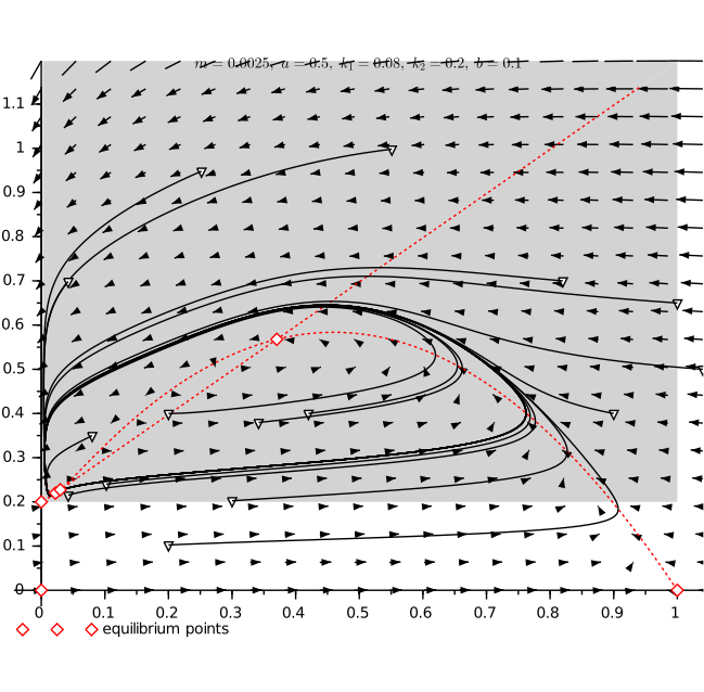
Figure 1: A phase portrait of (1.2) with three equilibrium points and a cycle in the interior of $\mathcal{A}$. The dashed lines are isoclines $y=\frac{x(1-x)(k_{1}+x-m)}{a(x-m)}$ and $y=k_{2}+x-m$. The grey region is the invariant attracting domain $\mathcal{A}$.
$m=0.0025$, $a=0.5$, $k_{1}=0.08$, $k_{2}=0.2$, $b=0.1$.

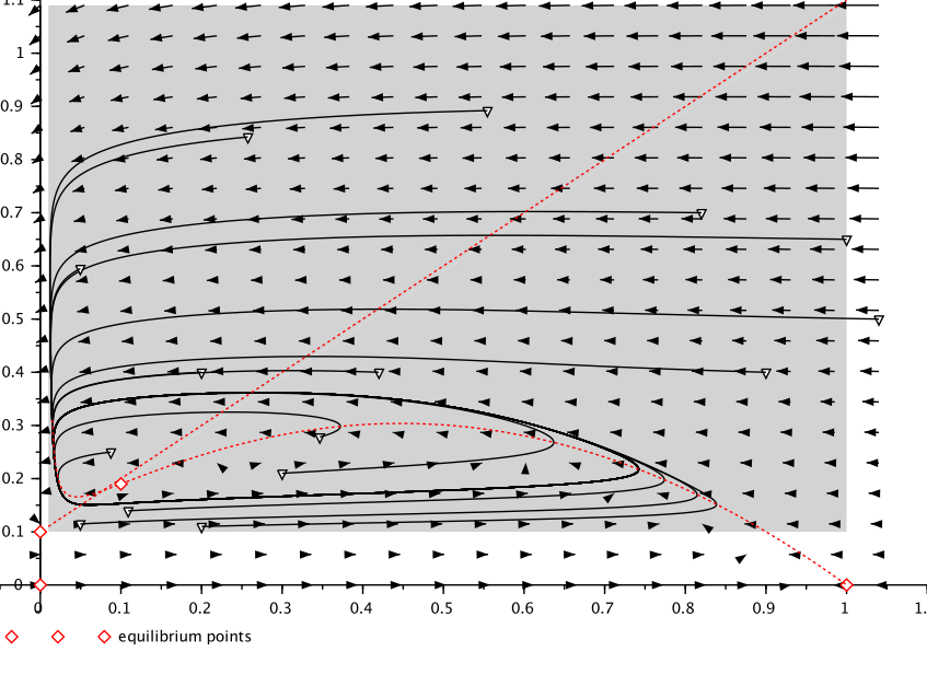
Figure 2: A phase portrait of (1.2) with an unstable equilibrium and a stable limit cycle.
$m=0.01$, $a=1$, $k_{1}=0.1$, $k_{2}=0.1$, $b=0.05$.

4.2 Stochastically perturbated system

We numerically simulate the solution to System (1.3). Using the Milstein scheme (see [19]), we consider the discretized system

(4.2) $$x_{k+1}= \ x_{k}+\left[{x_{k}(1-x_{k}-\frac{ay_{k}}{k_{1}+x_{k}-m})}\right]h+\sigma_{1}\,x_{k}\sqrt{h}\,\xi^{2}_{k}+\frac{1}{2}\sigma_{1}^{2}x_{k}(h\,\xi^{2}_{k}-h),$$

$$y_{k+1}= \,y_{k}+by_{k}\left[{1-\frac{y}{k_{2}+x}}\right]h+\sigma_{2}y_{k}\sqrt{h}\,\xi^{2}_{k}+\frac{1}{2}\sigma_{2}^{2}y_{k}(h\,\xi^{2}_{k}-h),$$

where $(\xi_{k})$ is an i.i.d. sequence of normalized centered Gaussian variables.

Simulations of the stochastically perturbated case are shown in Figure 4. These simulations show the permanence of the system (1.3).

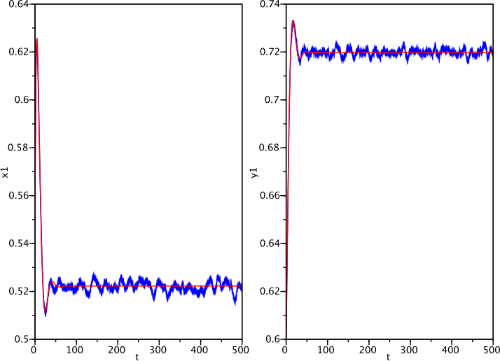
(a) $\sigma_{1}=0.01,\sigma_{2}=0.01$

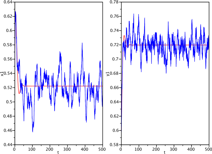
(b) $\sigma_{1}=0.3$, $\sigma_{2}=0.2$

Figure 4: Solutions to the stochastic system (1.3) and the corresponding deterministic system, represented respectively by the blue line and the red line.
$a=0.4$, $k_{1}=0.08$, $k_{2}=0.2$, $b=0.1$, $m=0.0025$, the initial value $(x(0),y(0))=(0.55,0.6),$ and the time step $h=0.01.$ The deterministic model has a globally stable equilibrium point $(x^{*},y^{*})=(0.55,0.75)$.

email address: slimani_safia@yahoo.fr
email address: prf@univ-rouen.fr
email address: islam.boussaada@l2s.centralesupelec.fr

References

- [1] W. Abid, R. Yafia, M. A. Aziz-Alaoui and A. Aghriche, Turing Instability and Hopf Bifurcation in a Modified Leslie–Gower Predator–Prey Model with Cross-Diffusion, Internat. J. Bifur. Chaos Appl. Sci. Engrg., 28 (2018), 1850089, 17, URL https://doi.org/10.1142/S021812741850089X.
- [2] W. Abid, R. Yafia, M. A. Aziz-Alaoui, H. Bouhafa and A. Abichou, Diffusion driven instability and Hopf bifurcation in spatial predator-prey model on a circular domain, Appl. Math. Comput., 260 (2015), 292–313, URL https://doi.org/10.1016/j.amc.2015.03.070.
- [3] M. A. Aziz-Alaoui and M. Daher Okiye, Boundedness and global stability for a predator-prey model with modified Leslie-Gower and Holling-type II schemes, Appl. Math. Lett., 16 (2003), 1069–1075, URL http://dx.doi.org/10.1016/S0893-9659(03)90096-6.
- [4] M. Bandyopadhyay and J. Chattopadhyay, Ratio-dependent predator-prey model: effect of environmental fluctuation and stability, Nonlinearity, 18 (2005), 913–936, URL https://doi.org/10.1088/0951-7715/18/2/022.
- [5] N. P. Bhatia and G. P. Szegö, Stability theory of dynamical systems, Die Grundlehren der mathematischen Wissenschaften, Band 161, Springer-Verlag, New York-Berlin, 1970.
- [6] B. I. Camara, Waves analysis and spatiotemporal pattern formation of an ecosystem model, Nonlinear Anal. Real World Appl., 12 (2011), 2511–2528, URL http://dx.doi.org/10.1016/j.nonrwa.2011.02.020.
- [7] F. Chen, L. Chen and X. Xie, On a Leslie-Gower predator-prey model incorporating a prey refuge, Nonlinear Anal. Real World Appl., 10 (2009), 2905–2908, URL http://dx.doi.org/10.1016/j.nonrwa.2008.09.009.
- [8] G. Da Prato and H. Frankowska, Stochastic viability of convex sets, J. Math. Anal. Appl., 333 (2007), 151–163, URL https://doi.org/10.1016/j.jmaa.2006.08.057.
- [9] M. Daher Okiye and M. A. Aziz-Alaoui, On the dynamics of a predator-prey model with the Holling-Tanner functional response, in Mathematical modelling & computing in biology and medicine, vol. 1 of Milan Res. Cent. Ind. Appl. Math. MIRIAM Proj., Esculapio, Bologna, 2003, 270–278.
- [10] N. Dalal, D. Greenhalgh and X. Mao, A stochastic model for internal HIV dynamics, J. Math. Anal. Appl., 341 (2008), 1084–1101, URL http://dx.doi.org/10.1016/j.jmaa.2007.11.005.
- [11] F. Dumortier, J. Llibre and J. C. Artés, Qualitative theory of planar differential systems, Universitext, Springer-Verlag, Berlin, 2006.
- [12] G. Ferreyra and P. Sundar, Comparison of solutions of stochastic equations and applications, Stochastic Anal. Appl., 18 (2000), 211–229, URL http://dx.doi.org/10.1080/07362990008809665.
- [13] J. Fu, D. Jiang, N. Shi, T. Hayat and A. Alsaedi, Qualitative analysis of a stochastic ratio-dependent Holling-Tanner system, Acta Math. Sci. Ser. B (Engl. Ed.), 38 (2018), 429–440, URL https://doi.org/10.1016/S0252-9602(18)30758-6.
- [14] F. R. Gantmacher, The theory of matrices. Vols. 1, 2, Translated by K. A. Hirsch, Chelsea Publishing Co., New York, 1959.
- [15] D. H. Gottlieb, A de Moivre like formula for fixed point theory, in Fixed point theory and its applications (Berkeley, CA, 1986), vol. 72 of Contemp. Math., Amer. Math. Soc., Providence, RI, 1988, 99–105, URL http://dx.doi.org/10.1090/conm/072/956481.
- [16] J. Guckenheimer and P. Holmes, Nonlinear oscillations, dynamical systems, and bifurcations of vector fields, vol. 42 of Applied Mathematical Sciences, Springer-Verlag, New York, 1983, URL http://dx.doi.org/10.1007/978-1-4612-1140-2.
- [17] C. Ji, D. Jiang and N. Shi, Analysis of a predator-prey model with modified Leslie-Gower and Holling-type II schemes with stochastic perturbation, J. Math. Anal. Appl., 359 (2009), 482–498, URL https://doi.org/10.1016/j.jmaa.2009.05.039.
- [18] R. Khasminskii, Stochastic stability of differential equations, vol. 66 of Stochastic Modelling and Applied Probability, 2nd edition, Springer, Heidelberg, 2012, URL http://dx.doi.org/10.1007/978-3-642-23280-0, With contributions by G. N. Milstein and M. B. Nevelson.
- [19] P. E. Kloeden and E. Platen, Numerical solution of stochastic differential equations, vol. 23 of Applications of Mathematics (New York), Springer-Verlag, Berlin, 1992, URL http://dx.doi.org/10.1007/978-3-662-12616-5.
- [20] P. H. Leslie and J. C. Gower, The properties of a stochastic model for the predator-prey type of interaction between two species, Biometrika, 47 (1960), 219–234, URL https://doi.org/10.1093/biomet/47.3-4.219.
- [21] L. Liu and Y. Shen, Sufficient and necessary conditions on the existence of stationary distribution and extinction for stochastic generalized logistic system, Adv. Difference Equ., 2015:10, 13, URL http://dx.doi.org/10.1186/s13662-014-0345-y.
- [22] Z. Liu, Stochastic dynamics for the solutions of a modified Holling-Tanner model with random perturbation, Internat. J. Math., 25 (2014), 1450105, 23, URL http://dx.doi.org/10.1142/S0129167X14501055.
- [23] J. Llibre and J. Villadelprat, A Poincaré index formula for surfaces with boundary, Differential Integral Equations, 11 (1998), 191–199.
- [24] J. Lv and K. Wang, Analysis on a stochastic predator-prey model with modified Leslie-Gower response, Abstr. Appl. Anal., Art. ID 518719, 16, URL http://dx.doi.org/10.1155/2011/518719.
- [25] J. Lv and K. Wang, Asymptotic properties of a stochastic predator-prey system with Holling II functional response, Commun. Nonlinear Sci. Numer. Simul., 16 (2011), 4037–4048, URL http://dx.doi.org/10.1016/j.cnsns.2011.01.015.
- [26] T. Ma and S. Wang, A generalized Poincaré-Hopf index formula and its applications to 2-D incompressible flows, Nonlinear Anal. Real World Appl., 2 (2001), 467–482, URL http://dx.doi.org/10.1016/S1468-1218(01)00004-9.
- [27] P. S. Mandal and M. Banerjee, Stochastic persistence and stability analysis of a modified Holling-Tanner model, Math. Methods Appl. Sci., 36 (2013), 1263–1280, URL http://dx.doi.org/10.1002/mma.2680.
- [28] R. M. May, Stability and Complexity in Model Ecosystems, Princeton University Press, Princeton, New Jersey, 1973.
- [29] A. F. Nindjin, M. A. Aziz-Alaoui and M. Cadivel, Analysis of a predator-prey model with modified Leslie-Gower and Holling-type II schemes with time delay, Nonlinear Anal. Real World Appl., 7 (2006), 1104–1118, URL https://doi.org/10.1016/j.nonrwa.2005.10.003.
- [30] E. C. Pielou, Mathematical ecology, 2nd edition, Wiley-Interscience [John Wiley & Sons], New York-London-Sydney, 1977.
- [31] C. C. Pugh, A generalized Poincaré index formula, Topology, 7 (1968), 217–226.
- [32] J. Tong, and , Math. Gaz., 88 (2004), 511–513.
- [33] R. Yafia and M. A. Aziz-Alaoui, Existence of periodic travelling waves solutions in predator prey model with diffusion, Appl. Math. Model., 37 (2013), 3635–3644, URL https://doi.org/10.1016/j.apm.2012.08.003.
- [34] R. Yafia, F. El Adnani and H. T. Alaoui, Limit cycle and numerical similations for small and large delays in a predator-prey model with modified Leslie-Gower and Holling-type II schemes, Nonlinear Anal. Real World Appl., 9 (2008), 2055–2067, URL https://doi.org/10.1016/j.nonrwa.2006.12.017.
- [35] R. Yafia, F. El Adnani and H. Talibi Alaoui, Stability of limit cycle in a predator-prey model with modified Leslie-Gower and Holling-type II schemes with time delay., Appl. Math. Sci., Ruse, 1 (2007), 119–131.