Recognizing Cuneiform Signs Using Graph Based Methods

Abstract

The cuneiform script constitutes one of the earliest systems of writing and is realized by wedge-shaped marks on clay tablets. A tremendous number of cuneiform tablets have already been discovered and are incrementally digitalized and made available to automated processing. As reading cuneiform script is still a manual task, we address the real-world application of recognizing cuneiform signs by two graph based methods with complementary runtime characteristics. We present a graph model for cuneiform signs together with a tailored distance measure based on the concept of the graph edit distance. We propose efficient heuristics for its computation and demonstrate its effectiveness in classification tasks experimentally. To this end, the distance measure is used to implement a nearest neighbor classifier leading to a high computational cost for the prediction phase with increasing training set size. In order to overcome this issue, we propose to use CNNs adapted to graphs as an alternative approach shifting the computational cost to the training phase. We demonstrate the practicability of both approaches in an experimental comparison regarding runtime and prediction accuracy. Although currently available annotated real-world data is still limited, we obtain a high accuracy using CNNs, in particular, when the training set is enriched by augmented examples.

1 Introduction

Besides the Egyptian hieroglyphs, the cuneiform script is the oldest writing system in the world. Since its emergence at the end of the 4th century BC the cuneiform writing system was in use for more than three millennia by various cultures (Rüster and Neu, 1989). It was eventually replaced by alphabetic writing systems, which were easier to learn. Cuneiform manuscripts were written predominantly on clay tablets, cf. fig:cuneiform_tablet. These tablets are an important source for revealing early human history, ranging from simple delivery notes over religious texts to contracts between empires. Cuneiform inscriptions were usually created by impressing an angular stylus into moist clay, resulting in signs consisting of tetrahedron shaped markings, called wedges (Fisseler et al., 2013), as shown in fig:cuneiform_wedge.

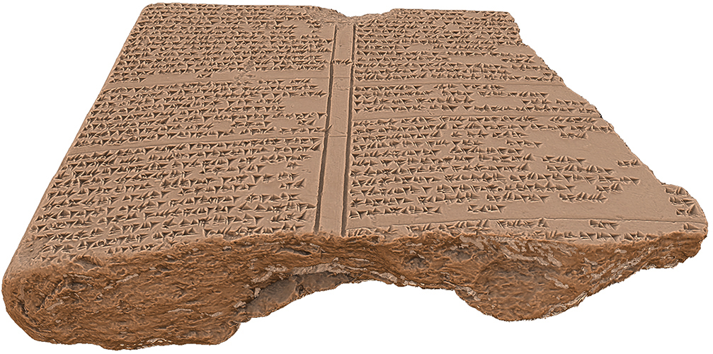
fig:cuneiform [Cuneiform tablet fragment] [Tetrahedron shaped markings]

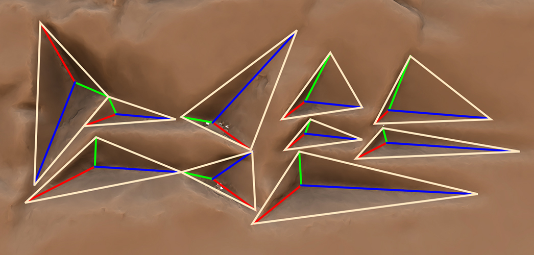
Figure 1: Example of a cuneiform tablet with tetrahedron shaped markings.

Over time, the inventory of cuneiform signs, i.e., groups of wedges, has been classified for various languages with values ranging from well over 1,000 signs for early cuneiform variants. For Hittite cuneiform, the visual appearance of wedges can be classified depending on the stylus orientation into vertical, horizontal and diagonal, so-called ‘Winkelhaken’ wedge types (Rüster and Neu, 1989). However, depending on the manuscripts state of conservation, it may not be possible to identify a wedge or sign solely based on its geometric appearance, but the geometric context in form of neighboring wedges and signs must also be considered.

Over 500,000 cuneiform fragments have been discovered so far and are digitalized with the help of high-resolution 3D measurement technologies (Rothacker et al., 2015). The resulting data provides a starting point for automated processing approaches to support philologists in their analysis. However, many script related aspects of the digitalized data are annotation-bound, as reading and analyzing cuneiform manuscripts is still a manual task, which is difficult and time consuming even for human experts. Due to the high data acquisition costs, classifiers need to be able to learn from a small number of examples and generalize well to a huge amount of unknown data.

1.1 Related work

We briefly summarize the related work on the cuneiform font metrology, the graph edit distance and geometric deep learning.

Cuneiform font metrology

Automated processing of digital cuneiform data can be conducted on a variety of representations, ranging from photographic reproductions to 3D scanned point clouds and derived representations. Fisseler et al. (2013) use a fault tolerant wedge extraction based on a tetrahedron model to create large amounts of data for statistical script analysis. This wedge model includes wedge component based features, like edges and depth points and a heuristic classification of wedge types. Based on generating 2D contour line vector representations of wedges, Bogacz et al. (2015a, b) proposed two approaches to classify cuneiform signs: One of them is based on graph representations, which are compared by graph kernels (Bogacz et al., 2015b), and the other computes the optimal assignment between vector representations (Bogacz et al., 2015a). Rothacker et al. (2015) proposed a Bag-of-Features and HMM based approach for automatically retrieving cuneiform structures on image representations from 3D scans.

Graph edit distance

Graph based methods have a long history in pattern recognition (Conte et al., 2004). In this domain, the graph edit distance has been proposed more than 30 years ago (Sanfeliu and Fu, 1983). Since then it has been proven to be a flexible method for error-tolerant graph matching with applications in numerous domains (Conte et al., 2004; Stauffer et al., 2017). Bunke (1997) has shown that computing the graph edit distance generalizes the classical maximum common subgraph problem, which is well known to be $\mathsf{NP}$-complete. Due to the high computational costs involved in solving such problems, the graph edit distance is usually not determined exactly in practice. Riesen and Bunke (2009) proposed a method to derive a series of edit operations from an optimal assignment between the vertices of the two input graphs. The method can be computed in cubic time, but not necessarily computes a minimum cost edit path from one graph to the other. However, the results have been shown to be sufficiently accurate for many applications (Stauffer et al., 2017). Recently, a binary linear programming formulation for computing the exact graph edit distance has been proposed (Lerouge et al., 2017). The method was shown to be efficient for several classes of real-world graphs with state-of-the art general purpose solvers.

Geometric deep learning

Upon the success of Convolutional Neural Networks (CNNs) on Euclidean domains with grid-based structured data, the generalization of CNNs on non-Euclidean domains, e.g., graphs or meshes, has drawn significant attention (Bronstein et al., 2017). Therefore, a set of methods emerged, which aim to extend the convolution operator in deep neural networks to handle irregular structured input data by preserving its main properties: local connectivity, weight sharing and shift invariance (LeCun et al., 1998).

Masci et al. (2015) introduced the first spatial mesh filtering approach by locally parameterizing the surface around each point using geodesic polar coordinates and defining convolutions on the resulting angular bins. Boscaini et al. (2016) improved this approach by introducing a patch rotation method to align extracted patches based on the local principal curvatures of the input manifold. Monti et al. (2017) proposed a method for continuous convolution kernels in the spatial domain by encoding spatial relations in edge attributes and using Gaussian kernels with trainable mean vector and covariance matrix as weight functions. Fey et al. (2018) introduced SplineCNN with continuous kernel functions based on B-splines, which make it possible to directly learn from the geometric structure of meshes.

1.2 Our contribution

We present two graph based methods for the classification of cuneiform signs represented by an original graph model. The first one compares two signs by the graph edit distance with a tailored cost function in order to implement a nearest neighbor classifier. The approach is able to take the relative relation between wedges into account and thereby overcomes limitations of approaches based on optimal assignments, where the costs are determined by the Euclidean distance in a global coordinate system. We present efficient problem-specific heuristics for finding suboptimal solutions, for which we show experimentally that they are sufficiently accurate for our application.

The second method employs the graph convolutional network SplineCNN. We show that augmentation on the training set, that is applying random affine transformation on vertex positions, yields significant improvements in accuracy. SplineCNN provides fast inference algorithms, so that graph neural networks offer a real alternative. We evaluate and compare both methods on a newly created, self-annotated graph based cuneiform dataset, which has been made publicly available to encourage further research.

2 Preliminaries

We consider directed graphs $G=(V,E)$, where $V$ are the vertices and $E\subseteq V\times V$ the edges. We allow vertices and edges to be annotated by arbitrary attributes or features and denote the $d$-dimensional position of the vertex $v_{i}$ by $\mathbf{p}_{i}\in\mathbb{R}^{d}$. For a vertex $v_{i}\in V$ its neighborhood set is denoted by $\set{N}(v_{i})$. We briefly recall the fundamentals of the two graph based techniques used for cuneiform recognition in the following.

2.1 Graph edit distance

The graph edit distance relies on the following elementary operations to edit a graph: vertex substitution, edge substitution, vertex deletion, edge deletion, vertex insertion and edge insertion. Each operation $o$ is assigned a cost $c(o)$, which may depend on the attributes associated with the affected vertices and edges. A sequence of edit operations $(o_{1},\dots,o_{k})$ that transforms a graph $G$ into another graph $H$ is called an edit path from $G$ to $H$. We denote the set of all possible edit paths from $G$ to $H$ by $\Upsilon(G,H)$. Let $G$ and $H$ be attributed graphs. The graph edit distance from $G$ to $H$ is defined by

$$d(G,H)=\min_{(o_{1},\dots,o_{k})\in\Upsilon(G,H)}\sum_{i=1}^{k}c(o_{i}).$$ (1)

In order to obtain a meaningful measure of dissimilarity for graphs, a cost function must be tailored to the particular attributes that are present in the considered graphs.

2.2 Graph convolutional network

For the graph convolutional network, we use SplineCNNs with their continuous spline-based convolution operator by Fey et al. (2018). SplineCNNs are a generalization of traditional CNNs for irregular structured data. For a graph $G$ with $n$ vertices we store the $m$ vertex attributes (without the positions) in a feature matrix $\mathbf{F}\in\mathbb{R}^{n\times m}$. Convolution over neighboring features for a vertex $v_{i}\in V$ is then defined by

$${(\mathbf{F}\star\mathbf{g})}_{i}=\frac{1}{|\set{N}(v_{i})|}\sum_{l=1}^{m}\sum_{v_{j}\in\set{N}(v_{i})}F_{j,l}\cdot g_{l}(\mathbf{p}_{i}-\mathbf{p}_{j}),$$ (2)

where $\mathbf{g}=(g_{1},\ldots,g_{m})$ defines $m$ continuous kernel functions, which weight the components of $\mathbf{F}_{j}$ based on the spatial relation $\mathbf{p}_{i}-\mathbf{p}_{j}$ between vertex $v_{i}$ and $v_{j}$. A kernel function $g_{l}$ is parameterized by a fixed number of trainable parameters. For computing $g_{l}(\mathbf{p}_{i}-\mathbf{p}_{j})$, the kernel function relies on the product of B-spline basis functions of a user-defined degree and can thus be evaluated very efficiently due to the local support property of B-splines. While training, the parameters of the convolution operator are optimized using gradient descent.

3 Representing cuneiform signs by graphs

The dataset used in this work has been generated using the approach of Fisseler et al. (2013) to automatically extract a tetrahedron based wedge model for individual wedges. The selected cuneiform tablets have been chosen to guarantee the inclusion of a sufficient number of individual cuneiform signs and a sufficient number of representatives for each class. As these requirements are difficult to meet on a small selection of ancient cuneiform fragments, we used a selection of nine cuneiform tablets written by scholars of Hittitology in the course of a study about individualistic characteristics of cuneiform hand writing. The tablets were provided by the Hethitologie-Portal Mainz (Müller, 2000). Each tablet contains up to 30 sylabic Hittite cuneiform signs, cf. fig:tablet, with each scribe contributing at least two tablets. This results in a total of nine samples and four different scribes for each sign. The signs were chosen to include either visually very distinctive wedge constellations and visually extremely similar signs. Therefore, the dataset includes both challenges to test the generalization and the discriminization capabilities of the methods. As the used segmentation approach extracts only individual wedge models, manual post-processing was applied to specify the affiliation of the wedges to the cuneiform signs.

3.1 Graph model

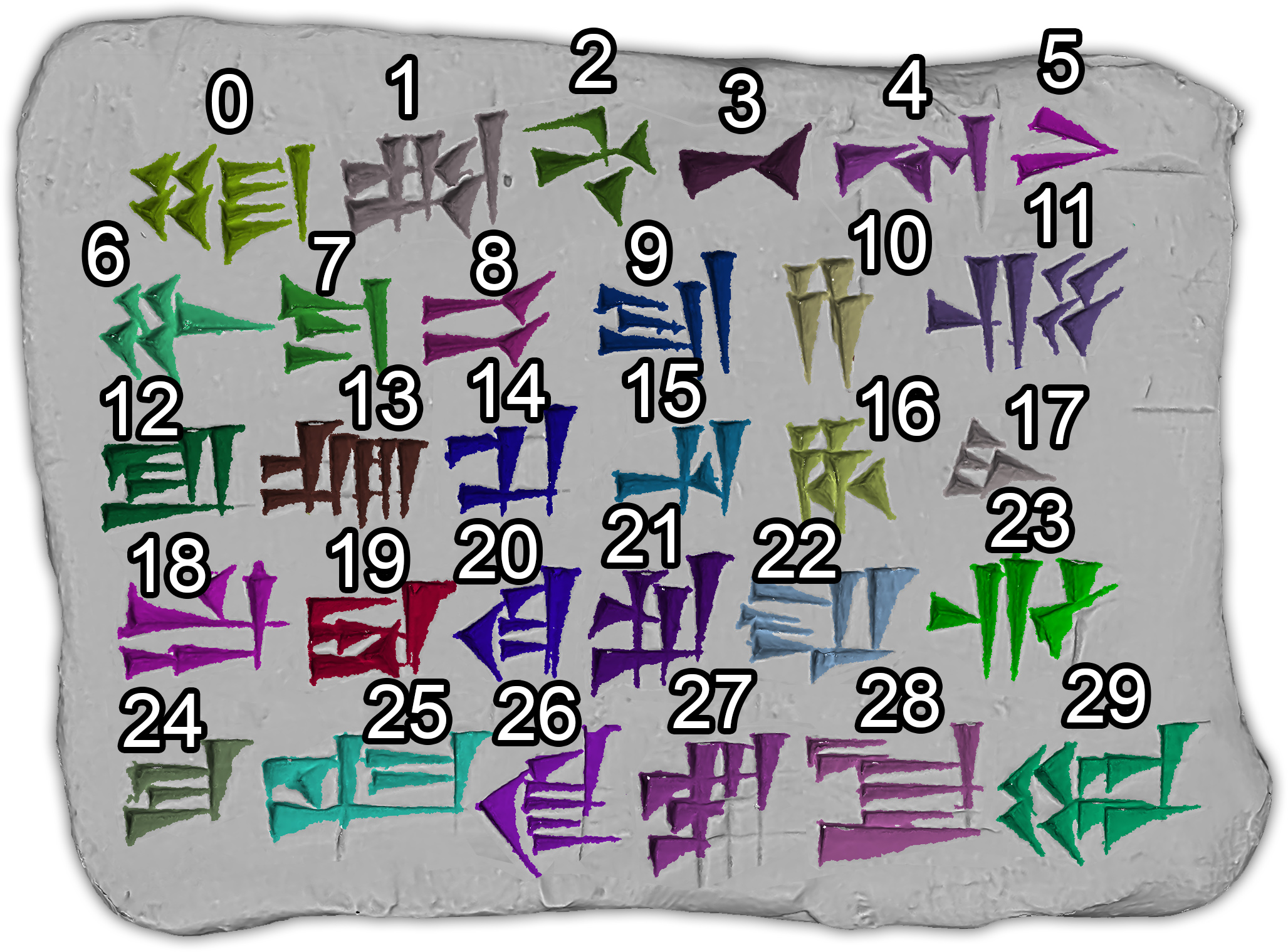
fig:tablet_graph [Cuneiform tablet] [Graph representation]

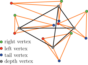
Figure 2: Cuneiform tablet and the graph representation of sign 2.

We represent each wedge by four vertices, which are labeled by their point (depth, tail, right, left) respectively glyph types (vertical, horizontal, ‘Winkelhaken’) and their spatial coordinates in $\mathbb{R}^{2}$. The vertices of the same wedge are pairwise adjacent and form a clique, as shown in fig:graph. The relative relation between individual wedges is not adequately modeled by their location in the global coordinate system. In fig:tablet the signs ‘tu’ (number 0) and ‘li’ (number 29) differ only by the arrangement of the four horizontal wedges, which are either ordered from top to bottom or arranged in a square. While this difference is easily recognized visually, the one sign can be turned into the other without shifting wedges far away. In order to obtain connected graphs we introduce additional edges between all pairs of depth vertices. These edges are also used to compare the relative positions of wedges and we refer to them as arrangement edges. In the following section we describe how arrangement edges are matched using the graph edit distance. Our experimental evaluation in sec:exp will show that these edges are crucial to obtain a meaningful distance in classification tasks for some cuneiform signs.

4 Comparing cuneiform signs using the graph edit distance

In order to obtain a meaningful distance measure for cuneiform graphs we employ the following cost function. The vertex substitution costs are $\infty$ for vertices with different labels (vertex type or glyph type) and the squared Euclidean distance between the associated coordinates otherwise. The costs for substituting arrangement edges are chosen to reflect the consistency of the relative relations between the associated wedges. Therefore, we annotate the arrangement edge $(v_{i},v_{j})$ by the Euclidean vector $\mathbf{p}_{j}-\mathbf{p}_{i}$. The cost for substituting an arrangement edge annotated by $\mathbf{x}$ for an arrangement edge annotated by $\mathbf{y}$ are then determined by the Cosine distance as $1-\mathbf{x}^{\top}\mathbf{y}/(\left\lVert\mathbf{x}\right\rVert\left\lVert\mathbf{y}\right\rVert)$ weighted by a parameter $\alpha$ in order to balance the influence of vertex and edge substitutions. The other edges are substituted at no cost; we forbid to substitute edges of different type by setting the cost function to $\infty$ in this case. In order to support error-tolerant graph matching, we allow vertex and edge deletion/insertion at a (typically high) cost of $D$. We exploit the characteristics of this cost function in order to find efficient heuristic solutions in the following.

4.1 Heuristics for computing the cuneiform graph edit distance

We present efficient heuristics for computing the edit distance between two cuneiform graphs. Riesen and Bunke (2009) proposed to derive a suboptimal edit path between graphs from an optimal assignment of their vertices, where the assignment costs encode the local edge structure.

Considering our graph model and cost function, we observe that the four vertices representing the same wedge in one graph must be mapped to the corresponding vertices of one wedge in the other graph to avoid high costs for deleting edges. This motivates to compute an optimal assignment between wedges to obtain an edit path. For computing the assignment we initially ignore the costs caused by substituting arrangement edges, but take them into account when computing the cost of the edit path derived from the assignment. In more detail, we proceed as follows: For two cuneiform graphs $G$ and $H$ with wedges $\set{A}=\{a_{1},\dots,a_{n}\}$ and $\set{B}=\{b_{1},\dots,b_{m}\}$, we create the assignment cost matrix $\mathbf{C}$ according to

$$\mathbf{C}=\begin{bmatrix}[cccc|cccc]c_{1,1}&c_{1,2}&\cdots&c_{1,m}&c_{1,\epsilon}&\infty&\cdots&\infty\\ c_{2,1}&c_{2,2}&\cdots&c_{2,m}&\infty&c_{2,\epsilon}&\ddots&\vdots\\ \vdots&\vdots&\ddots&\vdots&\vdots&\ddots&\ddots&\infty\\ c_{n,1}&c_{n,2}&\cdots&c_{n,m}&\infty&\cdots&\infty&c_{n,\epsilon}\\ \cline{1-8}\cr c_{\epsilon,1}&\infty&\cdots&\infty&0&0&\cdots&0\\ \infty&c_{\epsilon,2}&\ddots&\vdots&0&0&\ddots&\vdots\\ \vdots&\ddots&\ddots&\infty&\vdots&\ddots&\ddots&0\\ \infty&\cdots&\infty&c_{\epsilon,m}&0&\cdots&0&0\\ \end{bmatrix},$$ (3)

where $c_{i,j}$ denotes the cost of assigning the wedge $a_{i}$ to the wedge $b_{j}$ of the other sign, $c_{i,\epsilon}$ is the cost of deleting the wedge $a_{i}$ and $c_{\epsilon,j}$ the cost of inserting the wedge $b_{j}$. The cost for assigning two wedges is the sum of squared Euclidean distances between their vertices of the same type, if the wedges are of the same glyph type, and $\infty$ otherwise. Since the deletion (insertion) of a wedge involves at least the deletion (insertion) of four vertices and twelve directed edges, we set $c_{i,\epsilon}=c_{\epsilon,j}=16D$ for $i\in\{1,\dots,n\}$ and $j\in\{1,\dots,m\}$. It should be noted that the costs defined above do not take the deletion, insertion and substitution costs of arrangement edges into account.

We find the optimal assignment for the problem defined above in cubic time using the Hungarian method. From this approach we derive two approximation algorithms: First, we directly use the optimal assignment cost as an approximation of the graph edit distance (APX1). This approach ignores all costs caused by arrangement edges. The second approach (APX2) determines the mapping of vertices of $G$ and $H$ from the assignment of wedges and determines the associated edit path, which includes the substitution of arrangement edges. With this approach the exact cost of this (not necessarily optimal) edit path is used as an approximation of the graph edit distance. Comparing APX1 to APX2 allows us to evaluate the importance of the arrangement edges experimentally.

5 Classifying cuneiform graphs using graph convolutional networks

The used graph convolutional neural network takes 8-dimensional input features for each vertex and outputs a confidence distribution over the different cuneiform signs. Input features for a vertex are given by its point type (depth, tail, right and left) and glyph type (vertical, horizontal, ‘Winkelhaken’) as either $-1$ or $1$ as well as an additional $1$ for each vertex to be able to learn from the general geometry of cuneiform signs itself.

fig:network gives a comprehensive view of the used network architecture. The network consists of three convolutional layers and therefore aggregates local $3$-neighborhoods. We use Exponential Linear Units (ELUs) as non-linearities after each layer. In each layer, we extend the number of feature maps from 8 to 32 to finally 64 maps. For the spline-based convolution operator by Fey et al. (2018), we use a B-spline with degree of 1, which is parameterized by 25 trainable parameters. After that, we average features in the vertex dimension, which enables the use of a fully-connected layer from 64 to 30 neurons. Applying softmax, we obtain a confidence distribution over 30 different cuneiform signs.

fig:network

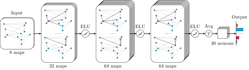
Figure 3: Graph convolutional network architecture for classifying 30 cuneiform signs.

5.1 Augmentation

We make heavy use of augmentation on the training set in order to reduce overfitting by applying random affine transformations on the graph vertices respectively graphs. Translation, scaling and rotation on a graph vertex with position $\mathbf{p}\in\mathbb{R}^{2}$ are therefore given by

$$\overline{\mathbf{p}}=\mathbf{p}+\begin{pmatrix}t_{1}\\ t_{2}\end{pmatrix},\quad\overline{\mathbf{p}}=\begin{pmatrix}s_{1}&0\\ 0&s_{2}\end{pmatrix}\cdot\mathbf{p},\quad\overline{\mathbf{p}}=\begin{pmatrix}\cos(\theta)&-\sin(\theta)\\ \sin(\theta)&\phantom{-}\cos(\theta)\end{pmatrix}\cdot\mathbf{p},$$ (4)

where $t_{1},t_{2}\in[-T,T]$, $s_{1},s_{2}\in[\frac{1}{S},S]$ and $\theta\in[-\Theta,\Theta]$ are randomly sampled within a given boundary. It should be noted that affine transformations are not commutative and one might also consider randomizing their order of application. Here, we use a fixed order by first rotating and scaling the whole graph and finally translating individual graph vertices.

6 Experimental evaluation

We are interested in answering the following questions:

Q1

Is the cuneiform graph edit distance with the suggested cost function a meaningful measure to compare cuneiform signs? How do the heuristics for computing the graph edit distance compare to exact methods in terms of runtime and solution quality?

Q2

How do CNNs perform in comparison to a nearest neighbor classifier using the cuneiform graph edit distance? How sensitive is the SplineCNN to the training set size?

Q3

How do both methods compare in terms of runtime? What is the impact of the training set size in practice?

6.1 Experimental setup

For all experiments, we used the dataset described in sec:dataset, which contains $267$ cuneiform signs with 5,680 vertices and 23,922 edges in total. A comprehensive overview of the dataset can be found in tab:dataset.

tab:dataset Class ‘ba’ ‘bi’ ‘bu’ ‘da’ ‘di’ ‘du’ ‘ha’ ‘hi’ ‘hu’ ‘ka’ ‘ki’ ‘ku’ ‘la’ ‘li’ ‘lu’ $\#G$ 9 9 9 9 9 9 9 9 9 9 9 9 9 9 9 $|V|$ 36 24 16 8 16 8 20 16 16 20 16 28 24 28 16 $|E|$ 180 102 60 26 60 26 80 60 60 80 60 126 102 126 60 $h_{\max}$ 7.5 7.4 10.0 5.3 7.5 7.7 7.3 7.9 7.5 9.1 9.1 7.4 7.7 6.7 7.5 $w_{\max}$ 12.7 11.7 13.4 7.3 14.7 8.7 13.9 10.0 9.4 11.1 5.8 13.7 11.4 10.6 15.0 Class ‘na’ ‘ni’ ‘nu’ ‘ra’ ‘ri’ ‘ru’ ‘sa’ ‘si’ ‘su’ ‘ta’ ‘ti’ ‘tu’ ‘za’ ‘zi’ ‘zu’ $\#G$ 9 9 9 9 9 9 9 9 9 9 9 9 8 8 8 $|V|$ 16 24 16 20 20 20 20 24 20 16 28 28 24 28 36 $|E|$ 60 102 60 80 80 80 80 102 80 60 126 126 102 126 180 $h_{\max}$ 8.5 9.9 10.2 7.7 8.9 8.2 10.0 9.2 8.2 8.3 12.6 10.5 9.1 8.9 10.3 $w_{\max}$ 14.4 7.6 8.6 9.6 11.5 10.2 10.4 11.2 11.7 8.4 15.2 12.4 9.2 13.2 21.0

Table 1: Dataset characteristics for all 30 classes: Number of graphs $\#G$, vertices $|V|$, edges $|E|$ and the maximum height $h_{\max}$ and width $w_{\max}$ of the axis-aligned minimum bounding boxes.

Edit distance

We implemented an exact method for computing the graph edit distance based on a recent binary linear programming formulation (Lerouge et al., 2017) and solved all instances using Gurobi v7.5.2. The exact method as well as the two heuristics were implemented in Java. The experiments were conducted using Java v1.8.0 on an Intel Core i7-3770 CPU at 3.4GHz with 16GB of RAM using a single processor only. We set the parameters $\alpha=1000$ and $D=1000$.

Graph convolutional network

We trained the proposed SplineCNN architecture on a single NVIDIA GTX 1080 Ti with 11GB of memory using PyTorch. Each experiment was trained for 300 epochs using Adam optimization (Kingma and Ba, 2015) and cross entropy loss, with a batch size of 32, dropout probability of 0.5, an initial learning rate of 0.01 and learning rate decay to 0.001 after 200 epochs. Hyperparameters for augmentation were set to $T=0.1$, $S=1.4$ and $\Theta=0.6$.

6.2 Evaluation of the cuneiform graph edit distance (Q1)

We compared the exact method and the two heuristics APX1 and APX2 described in sec:ged:apx. We used the signs of one tablet as a reference and, for each reference sign, sorted all the elements of the dataset according to their distance to the reference sign. We expect that the other instances of the same sign have a small distance and populate the top ranks. We consider a classifier which assigns the top $k$ elements in the ranking to the same class as the reference sign and considered the ROC curves obtained for varying $k$.

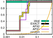
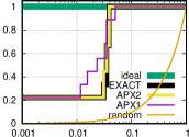
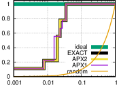
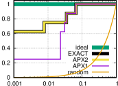
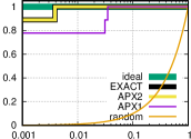
fig:roc_selection [Sign ‘ba’] [Sign ‘ki’] [Sign ‘ku’] [Sign ‘li’] [Sign ‘ni’] [Sign ‘tu’]

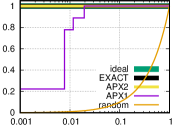
Figure 4: Selected ROC curves for the ranking experiments.

We obtained ideal results (AUC 1) for 16 of 30 signs by all three methods, i.e., most signs are perfectly recognized by APX1, APX2 and the exact method. fig:roc_selection shows a selection of the resulting ROC curves for more challenging signs, see Appendix A for a complete overview. Please note the logarithmic scale of the $x$-axis. fig:roc_selection:ba and fig:roc_selection:ku show a clear deviation from the ideal. The reason for this is that the signs ‘ba’ and ‘ku’ are often not correctly distinguished and have a small distance. On a purely geometric level without semantic context, these signs are difficult to distinguish even for human experts, see signs number 7 and 24 in fig:tablet. APX1 and APX2 both perform well in most cases. However, in order to distinguish ‘li’ and ‘tu’ the relative relation between wedges has to be taken into account, see signs number 0 and 29 in fig:tablet. For these two signs we observe that APX2 indeed outperforms APX1, cf. fig:roc_selection:li and fig:roc_selection:tu. The poor performance for the sign ‘ki’, cf. fig:roc_selection:ki, can be explained by the fact that the reference sign contains a scribal error on the reference tablet. fig:roc_selection:ni is a typical example showing a satisfying performance, where only very few instances of the reference signs were ranked slightly below other signs. In almost all experiments we observed that APX2 leads to the same ROC curve as the exact method. Moreover, we verified that both compute the same distance with very few exceptions primarily for examples widely separated.

The average runtime for computing the rankings for all 30 signs, which involves more than 80,000 distance computations, was 27.27 minutes for the exact method, 48.7 milliseconds for APX1 and 53.7 milliseconds for APX2. In summary, we have shown that the cuneiform graph edit distance provides an adequate measure for the comparison and recognition of cuneiform signs and can be efficiently approximated by APX2 without sacrificing accuracy.

6.3 Classification via edit distance and SplineCNN (Q2)

We performed $10$-fold cross validation on random splits of the dataset in order to provide a fair comparison. For SplineCNN, the accuracy for each split is given by the average over 10 experiments due to random uniform weight initialization. For the cuneiform graph edit distance we used a $3$-nearest neighbors classifier on the same splits. The accuracy results are summarized in Table LABEL:tab:results.

tab:results # Split Method Mean 1 2 3 4 5 6 7 8 9 10 GED EXACT 93.24 96.30 100.0 96.30 100.0 92.59 85.19 85.19 85.19 100.0 91.67 $\pm$ 5.94 GED APX1 89.17 92.59 96.30 96.30 88.89 85.19 81.48 81.48 81.48 96.30 91.67 $\pm$ 6.03 GED APX2 92.87 92.59 100.0 96.30 100.0 92.59 85.19 85.19 85.19 100.0 91.67 $\pm$ 5.86 CNN without 87.37 86.56 86.30 87.41 90.74 92.60 93.33 87.04 79.26 81.48 90.00 augmentation $\pm$ 6.16 $\pm$ 4.43 $\pm$ 3.92 $\pm$ 5.84 $\pm$ 6.11 $\pm$ 4.62 $\pm$ 2.92 $\pm$ 3.15 $\pm$ 5.00 $\pm$ 3.90 $\pm$ 4.89 CNN with 93.54 95.92 94.81 100.0 94.44 95.19 89.63 90.74 88.89 99.37 95.42 augmentation $\pm$ 4.40 $\pm$ 2.73 $\pm$ 2.59 $\pm$ 0.00 $\pm$ 3.15 $\pm$ 1.79 $\pm$ 2.92 $\pm$ 4.00 $\pm$ 4.62 $\pm$ 1.91 $\pm$ 3.65

Table 2: Cuneiform sign classification results of all proposed methods for each test split, overall mean accuracy and standard deviation.

The graph edit distance based classifiers provide a high classification accuracy. The exact method and APX2 both outperform APX1, which can be explained by the impact of arrangement edges. For SplineCNN, we obtain high accuracies, although deep learning is well known for demanding a huge amount of training data. We can even beat the proposed approaches by a small margin with the use of augmentation, that is generating augmented examples in each epoch, which differ from the training data by a random affine transformation. However, choosing a smaller amount of training data yields lower results due to an decrease in training and an increase in test data size. For example, on a pre-chosen 50/50 split, we obtain an accuracy of 90.23%, resulting in a quite sensitive approach to the training set size. Moreover, it is worth pointing out that the output accuracies of different test splits can yield quite varying results. This can be traced back to the small number of test graphs, approximately 27, where a single false classification leads to jumps in accuracy of approximately 3.70 percentage points.

It can be further observed that there exist a few test splits, where the exact method and APX2 both outperform APX1 and SplineCNN, cf. split 4. This indicates that SplineCNN faces difficulties identifying characters where arrangement edges play a crucial role. This behaviour might be explained by the uniform knot vectors of the B-spline kernels, as the kernel functions lose granular control for neighborhoods with very long as well as very short edges.

In summary, all methods provide a high classification accuracy with the SplineCNN performing best when the training set is augmented.

6.4 Evaluation of runtimes (Q3)

We experimentally evaluated the runtime of both methods for training and testing with varying dataset sizes. We report the runtimes averaged over 10 runs for SplineCNN, APX1 and APX2. For the nearest neighbor classifier no training is required and we report the prediction time for a fixed test set using training sets of varying size. tab:runtime summarizes the results. The runtimes generally grow linearly with the number of graphs in the training and test set. For SplineCNN, the runtime to train all 267 cuneiform signs is 6.7 seconds, whereas the runtime for classifying all signs is very fast with approximately 14 milliseconds. Classification using the exact method is very slow in practice, while APX1 and APX2 both are fast for our dataset. However, since their prediction time increases with the training set size these approaches can be expected to become less feasible when the available training data grows.

tab:runtime[SplineCNN] Size [%] Training [s] Test [ms] 25 $1.95\pm 0.02$ $3.56\pm 0.18$ 50 $3.51\pm 0.03$ $7.31\pm 0.49$ 75 $5.08\pm 0.01$ $11.46\pm 0.89$ 100 $6.66\pm 0.03$ $13.99\pm 0.39$   [GED] Size [%] EXACT [s] APX1 [ms] APX2 [ms] 25 1301.1 $52.8\pm 1.17$ $56.5\pm 2.94$ 50 2617.3 $108.2\pm 11.4$ $110.6\pm 1.74$ 75 4008.3 $153.1\pm 2.43$ $165.4\pm 5.04$ 100 5407.8 $204.5\pm 2.42$ $222.2\pm 8.36$

Table 3: Runtime analysis of the used SplineCNN architecture for varying training and test sizes ($a$) and for classifying 50% of the signs by the graph distance based nearest neighbor classifier for varying training set sizes ($b$).

7 Conclusion and future work

We have proposed two complementary graph based methods for the recognition of cuneiform signs, which yield a first step towards supporting philologists in their analysis. We have evaluated our methods on a newly created real-world dataset w.r.t. runtime and classification accuracy. While both methods obtain high accuracy and efficiency, CNN based approaches might be advantageous when the available training data grows.

For future work, we would like to investigate our methods in the presence of scanning errors and extend our dataset by cuneiform signs that can only be distinguished in context. For neural networks, a traditional approach for recognizing those would be the addition of recurrent modules.

This research was supported by the German Science Foundation (DFG) within the Collaborative Research Center SFB 876 ‘Providing Information by Resource-Constrained Data Analysis’, project A6. We thank our colleges from the Hethitologie-Portal Mainz (Müller, 2000) for providing the scanned cuneiform tablets and for supporting us with their philological expertise. We are also thankful to Jan Eric Lenssen and Pascal Libuschewski for proofreading and helpful advice.

Appendix A ROC curves for rankings based on the graph edit distance

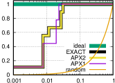
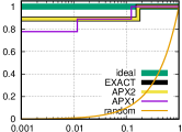
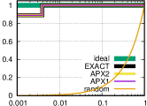
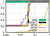
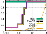
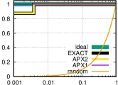
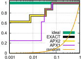
fig:roc1 [Sign ‘ba’] [Sign ‘bi’] [Sign ‘bu’] [Sign ‘da’] [Sign ‘di’] [Sign ‘du’] [Sign ‘ha’] [Sign ‘hi’] [Sign ‘hu’] [Sign ‘ka’] [Sign ‘ki’] [Sign ‘ku’] [Sign ‘la’] [Sign ‘li’] [Sign ‘lu’]

Figure 5: ROC curves for the ranking experiments (1/2).

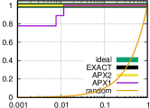
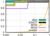
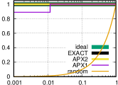
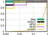
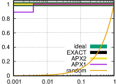
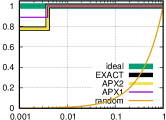
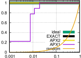
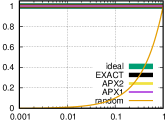
fig:roc2 [Sign ‘na’] [Sign ‘ni’] [Sign ‘nu’] [Sign ‘ra’] [Sign ‘ri’] [Sign ‘ru’] [Sign ‘sa’] [Sign ‘si’] [Sign ‘su’] [Sign ‘ta’] [Sign ‘ti’] [Sign ‘tu’] [Sign ‘za’] [Sign ‘zi’] [Sign ‘zu’]

Figure 6: ROC curves for the ranking experiments (2/2).

References

- Bogacz et al. (2015a) B. Bogacz, M. Gertz, and H. Mara. Cuneiform character similarity using graph representations. In Computer Vision Winter Workshop, 2015a.
- Bogacz et al. (2015b) B. Bogacz, M. Gertz, and H. Mara. Character retrieval of vectorized cuneiform script. In International Conference on Document Analysis and Recognition, 2015b.
- Boscaini et al. (2016) D. Boscaini, J. Masci, E. Rodolà, and Bronstein M. Learning shape correspondence with anisotropic convolutional neural networks. In Neural Information Processing Systems, 2016.
- Bronstein et al. (2017) M. M. Bronstein, J. Bruna, Y. LeCun, A. Szlam, and P. Vandergheynst. Geometric deep learning: Going beyond euclidean data. In IEEE Signal Processing Magazine, 2017.
- Bunke (1997) H. Bunke. On a relation between graph edit distance and maximum common subgraph. Pattern Recognition Letters, 1997.
- Conte et al. (2004) D. Conte, P. Foggia, C. Sansone, and M. Vento. Thirty years of graph matching in pattern recognition. International Journal of Pattern Recognition and Artificial Intelligence, 2004.
- Fey et al. (2018) M. Fey, J. E. Lenssen, F. Weichert, and H. Müller. SplineCNN: Fast geometric deep learning with continuous B-spline kernels. In Computer Vision and Pattern Recognition, 2018.
- Fisseler et al. (2013) D. Fisseler, F. Weichert, M. Cammarosano, and G. Müller. Towards an interactive and automated script feature analysis of 3D scanned cuneiform tablets. In Scientific Computing and Cultural Heritage, 2013.
- Kingma and Ba (2015) D. P. Kingma and J. L. Ba. Adam: A method for stochastic optimization. In International Conference on Learning Representations, 2015.
- LeCun et al. (1998) Y. LeCun, L. Bottou, Y. Bengio, and P. Haffner. Gradient-based learning applied to document recognition. In Proceedings of the IEEE, 1998.
- Lerouge et al. (2017) J. Lerouge, Z. Abu-Aisheh, R. Raveaux, P. Héroux, and S. Adam. New binary linear programming formulation to compute the graph edit distance. Pattern Recognition, 2017.
- Masci et al. (2015) J. Masci, D. Boscaini, M. M. Bronstein, and P. Vandergheynst. Geodesic convolutional neural networks on riemannian manifolds. In 3dRR, 2015.
- Monti et al. (2017) F. Monti, D. Boscaini, J. Masci, E. Rodolà, J. Svoboda, and M. M. Bronstein. Geometric deep learning on graphs and manifolds using mixture model CNNs. In Computer Vision and Pattern Recognition, 2017.
- Müller (2000) G. Müller. Hethitologie-Portal Mainz, 2000. URL http://www.hethiter.net. Akademie der Wissenschaften und Literatur Mainz (ADWM), and Julius-Maximilians-Universität Würzburg.
- Riesen and Bunke (2009) K. Riesen and H. Bunke. Approximate graph edit distance computation by means of bipartite graph matching. Image and Vision Computing, 2009.
- Rothacker et al. (2015) L. Rothacker, D. Fisseler, G. Müller, F. Weichert, and G. Fink. Retrieving cuneiform structures in a segmentation-free work spotting framework. In International Workshop on Historical Document Imaging and Processing, 2015.
- Rüster and Neu (1989) C. Rüster and E. Neu. Hethitisches Zeichenlexikon: Inventar und Interpretation der Keilschriftzeichen aus den Boğazköy-Texten. Studien zu den Boğazköy-Texten. O. Harrassowitz, 1989.
- Sanfeliu and Fu (1983) A. Sanfeliu and K. S. Fu. A distance measure between attributed relational graphs for pattern recognition. IEEE Transactions on Systems, Man, and Cybernetics, 1983.
- Stauffer et al. (2017) M. Stauffer, T. Tschachtli, A. Fischer, and K. Riesen. A survey on applications of bipartite graph edit distance. In Graph-Based Representations in Pattern Recognition, 2017.