Deep Generative Model for Joint Alignment and Word Representation

Abstract

This work exploits translation data as a source of semantically relevant learning signal for models of word representation. In particular, we exploit equivalence through translation as a form of distributed context and jointly learn how to embed and align with a deep generative model. Our EmbedAlign model embeds words in their complete observed context and learns by marginalisation of latent lexical alignments. Besides, it embeds words as posterior probability densities, rather than point estimates, which allows us to compare words in context using a measure of overlap between distributions (e.g. $\operatorname{KL}$ divergence). We investigate our model’s performance on a range of lexical semantics tasks achieving competitive results on several standard benchmarks including natural language inference, paraphrasing, and text similarity.

1 Introduction

Natural language processing applications often count on the availability of word representations trained on large textual data as a means to alleviate problems such as data sparsity and lack of linguistic resources (Collobert et al., 2011; Socher et al., 2011; Tu et al., 2017; Bowman et al., 2015).

Traditional approaches to inducing word representations circumvent the need for explicit semantic annotation by capitalising on some form of indirect semantic supervision. A typical example is to fit a binary classifier to detect whether or not a target word is likely to co-occur with neighbouring words (Mikolov et al., 2013). If the binary classifier represents a word as a continuous vector, that vector will be trained to be discriminative of the contexts it co-occurs with, and thus words in similar contexts will have similar representations.

The underlying assumption is that context (e.g. neighbouring words) stands for the meaning of the target word (Harris, 1954; Firth, 1957). The success of this distributional hypothesis hinges on the definition of context and different models are based on different definitions. Importantly, the nature of the context determines the range of linguistic properties the representations may capture (Levy and Goldberg, 2014b). For example, Levy and Goldberg (2014a) propose to use syntactic context derived from dependency parses. They show that their representations are much more discriminative of syntactic function than models based on immediate neighbourhood (Mikolov et al., 2013).

In this work, we take lexical translation as indirect semantic supervision (Diab and Resnik, 2002). Effectively we make two assumptions. First, that every word has a foreign equivalent that stands for its meaning. Second, that we can find this equivalent in translation data through lexical alignments. For that we induce both a latent mapping between words in a bilingual sentence pair and distributions over latent word representations.

To summarise our contributions:

• we model a joint distribution over sentence pairs that generates data from latent word representations and latent lexical alignments;

• we embed words in context mining positive correlations from translation data;

• we find that foreign observations are necessary for generative training, but test time predictions can be made monolingually;

• we apply our model to a range of semantic natural language processing tasks showing its usefulness.

2 EmbedAlign

In a nutshell, we model a distribution over pairs of sentences expressed in two languages, namely, a language of interest L1, and an auxiliary language L2 which our model uses to mine some learning signal. Our model, EmbedAlign, is governed by a simple generative story:

1. sample a length $m$ for a sentence in L1 and a length $n$ for a sentence in L2;

2. generate a sequence $z_{1},\ldots,z_{m}$ of $d$-dimensional random embeddings by sampling independently from a standard Gaussian prior;

3. generate a word observation $x_{i}$ in the vocabulary of L1 conditioned on the random embedding $z_{i}$;

4. generate a sequence $a_{i},\ldots,a_{n}$ of $n$ random alignments—each maps from a position $a_{j}$ in $x_{1}^{m}$ to a position $j$ in the L2 sentence;

5. finally, generate an observation $y_{j}$ in the vocabulary of L2 conditioned on the random embedding $z_{a_{j}}$ that stands for $x_{a_{j}}$.

The model is parameterised by neural networks and parameters are estimated to maximise a lowerbound on log-likelihood of joint observations. In the following, we present the model formally (§2.1), discuss efficient training (§2.2), and concrete architectures (§2.3).

2.1 Probabilistic model

Figure 1: A sequence $x_{1}^{m}$ is generated conditioned on a sequence of random embeddings $z_{1}^{m}$; generating the foreign sequence $y_{1}^{n}$ further requires latent lexical alignments $a_{1}^{n}$.

Notation

We use block capitals (e.g. $X$) for random variables, lowercase letters (e.g. $x$) for assignments, and the shorthand $X_{1}^{m}$ for a sequence $X_{1},\ldots,X_{m}$. Boldface letters are reserved for deterministic vectors (e.g. $\mathbf{v}$) and matrices (e.g. $\mathbf{W}$). Finally, $\mathbb{E}[f(Z);\alpha]$ denotes the expected value of $f(z)$ under a density $q(z|\alpha)$.

We model a joint distribution over bilingual parallel data, i.e., L1–L2 sentence pairs. An observation is a pair of random sequences $\langle X_{1}^{m},Y_{1}^{n}\rangle$, where a random variable $X$ ($Y$) takes on values in the vocabulary of L1 (L2). For ease of exposition, the length $m$ ($n$) of each sequence is assumed observed throughout. The L1 sentence is generated one word at a time from a random sequence of latent embeddings $Z_{1}^{m}$, each $Z$ taking on values in $\mathbb{R}^{d}$. The L2 sentence is generated one word at a time given a random sequence of latent alignments $A_{1}^{n}$, where $A_{j}\in\{1,\dotsc,m\}$ is the position in the L1 sentence to which $y_{j}$ aligns.

For $i\in\{1,\ldots,m\}$ and $j\in\{1,\ldots,n\}$ the generative story is

$$Z_{i} \sim\mathcal{N}(\mathbf{0},\mathbf{I})$$ (1a)

$$X_{i}|z_{i} \sim\operatorname{Cat}(f(z_{i};\theta))$$ (1b)

$$A_{j}|m \sim\mathcal{U}(1/m)$$ (1c)

$$Y_{j}|z_{1}^{m},a_{j} \sim\operatorname{Cat}(g(z_{a_{j}};\theta))$$ (1d)

and Figure 1 is a graphical depiction of our model. We map from latent embeddings to categorical distributions over either vocabulary using a neural network whose parameters are deterministic and collectively denote by $\theta$ (the generative parameters). The marginal likelihood of a sentence pair is shown in Equation (2).

$$P_{\theta}(x_{1}^{m},y_{1}^{n}|m,n)=\int p(z_{1}^{m})\prod_{i=1}^{m}P_{\theta}(x_{i}|z_{i})$$ (2)

$$\times\prod_{j=1}^{n}\sum_{a_{j}=1}^{m}P(a_{j}|m)P_{\theta}(y_{j}|z_{a_{j}})\differential z_{1}^{m}$$

Due to the conditional independences of our model, it is trivial to marginalise lexical alignments for any given latent embeddings $z_{1}^{m}$, but marginalising the embeddings themselves is intractable. Thus, we employ amortised mean field variational inference using the inference model

$$q_{\phi}(z_{1}^{m}|x_{1}^{m})\triangleq\prod_{i=1}^{m}\mathcal{N}(z_{i}|\mathbf{u}_{i},\operatorname{diag}(\mathbf{s}_{i}\odot\mathbf{s}_{i}))$$ (3)

where each factor is a diagonal Gaussian. We map from $x_{1}^{m}$ to a sequence $\mathbf{u}_{1}^{m}$ of independent posterior mean (or location) vectors, where $\mathbf{u}_{i}\triangleq\mu(\mathbf{h}_{i};\phi)$, as well as a sequence $\mathbf{s}_{1}^{m}$ of independent standard deviation (or scale) vectors, where $\mathbf{s}_{i}\triangleq\sigma(\mathbf{h}_{i};\phi)$, and $\mathbf{h}_{1}^{m}=\mathrm{enc}(x_{1}^{m};\phi)$ is a deterministic encoding of the L1 sequence (we discuss concrete architectures in §2.3). All mappings are realised by neural networks whose parameters are collectively denoted by $\phi$ (the variational parameters). Note that we choose to approximate the posterior without conditioning on $y_{1}^{n}$. This allows us to use the inference model for monolingual prediction in absence of L2 data.

Variational $\phi$ and generative $\theta$ parameters are jointly point-estimated to attain a local optimum of the evidence lowerbound (Jordan et al., 1999):

$$\log P_{\theta}(x_{1}^{m},y_{1}^{n}|m,n)\geq$$ (4)

$$\sum_{i=1}^{m}\mathbb{E}\left[\log P_{\theta}(x_{i}|Z_{i});\mathbf{u}_{i},\mathbf{s}_{i}\right]$$

$$+\sum_{j=1}^{n}\mathbb{E}\left[\log\sum_{a_{j}=1}^{m}P(a_{j}|m)P_{\theta}(y_{j}|Z_{a_{j}});\mathbf{u}_{1}^{m},\mathbf{s}_{1}^{m}\right]$$

$$-\sum_{i=1}^{m}\operatorname{KL}\left[\mathcal{N}(\mathbf{u}_{i},\operatorname{diag}(\mathbf{s}_{i}\odot\mathbf{s}_{i}))||\mathcal{N}(\mathbf{0},\mathbf{I})\right]\quad.$$

The variational family is location-scale, thus we can rely on stochastic optimisation (Robbins and Monro, 1951) and automatic differentiation (Baydin et al., 2015) with reparameterised gradient estimates (Kingma and Welling, 2014; Rezende et al., 2014; Titsias and Lázaro-Gredilla, 2014). Moreover, because the Gaussian density is an exponential family, the $\operatorname{KL}$ terms in (4) are available in closed-form (Kingma and Welling, 2014, Appendix B).

2.2 Efficient training

The likelihood terms in the ELBO (4) require evaluating two $\operatorname{softmax}$ layers over rather large vocabularies. This makes training prohibitively slow and calls for efficient approximation. We employ an approximation proposed by Botev et al. (2017) termed complementary sum sampling (CSS), which we review in this section.

Consider the likelihood term $\log P(X=\mathsf{x}|z)$ that scores an observation $\mathsf{x}$ given a sampled embedding $z$—we use serif font $\mathsf{x}$ to distinguish a particular observation from an arbitrary event $x\in\mathcal{X}$ in the support. The exact class probability

$$P(X=\mathsf{x}|z)=\frac{\exp(u(z,\mathsf{x}))}{\sum_{x\in\mathcal{X}}\exp(u(z,x))}$$ (5)

requires a normalisation over the complete support. CSS works by splitting the support into two sets, a set $\mathcal{C}$ that is explicitly summed over and must include the positive class $\mathsf{x}$, and another set $\mathcal{N}$ that is a subset of the complement set $\mathcal{X}\setminus C$. We obtain an estimate for the normaliser

$$\sum_{x\in\mathcal{C}}\exp(u(z,x))+\sum_{x\in\mathcal{N}}\kappa(x)\exp(u(z,x))$$ (6)

by importance- or Bernoulli-sampling from the support using a proposal distribution $Q(X)$, where $\kappa(x)$ corrects for bias as $\mathcal{N}$ tends to the entire complement set. In this paper, we design $\mathcal{C}$ and $\mathcal{N}$ per training mini-batch: we take $\mathcal{C}$ to consist of all unique words in a mini-batch of training samples and $\mathcal{N}$ to consist of $10^{3}$ negative classes uniformly sampled from the complement set $\mathcal{X}\setminus\mathcal{C}$, in which case $\kappa(x)=10^{-3}|\mathcal{X}\setminus\mathcal{C}|$.

CSS makes it particularly easy to approximate likelihood terms such as those with respect to L2 in Equation (4). Because those terms depend on a marginalisation over alignments, an approximation must give support to all words in the sequence $y_{1}^{n}$. With CSS this is extremely simple, we just need to make sure all unique words in $y_{1}^{n}$ are in the set $\mathcal{C}$—which our mini-batch procedure does guarantee. Botev et al. (2017) show that CSS is rather stable and superior to the most popular $\operatorname{softmax}$ approximations. Besides being simple to implement, CSS also addresses a few problems with other approximations. To name a few: unlike importance sampling approximations, CSS converges to the exact $\operatorname{softmax}$ with bounded computation (it takes as many samples as there are classes). Unlike hierarchical $\operatorname{softmax}$, CSS only affects training, that is, at test time we simply use the entire support instead of the approximation.

Without a $\operatorname{softmax}$ approximation, inference for our model would take time proportional to $O(m\times{v_{\texttt{x}}}+m\times{v_{\texttt{y}}}+m\times n)$ where ${v_{\texttt{x}}}$ (${v_{\texttt{y}}}$) corresponds to the size of the vocabulary of L1 (L2). The first term ($m\times{v_{\texttt{x}}}$) corresponds to projecting from $m$ latent embeddings to $m$ categorical distributions over the vocabulary of L1. The second term ($m\times{v_{\texttt{y}}}$) corresponds to projecting the same $m$ latent embeddings to $m$ categorical distributions over the vocabulary of L2. Finally, the third term ($m\times n$) is due to marginalisation of alignments. Note, however, that with the CSS approximation we drop the dependency on vocabulary sizes (as the combined sizes of $\mathcal{C}$ and $\mathcal{N}$ is an independent constant). Moreover, if inference is performed on GPU, the squared term ($m\times n\approx m^{2}$) is amortised due to parallelism. Thus, while training our model is somewhat slower than monolingual models of word representation, which typically run in $O(m)$, it is not at all impracticably slower.

2.3 Architectures

Here we present the neural network architectures that parameterise the different generative and variational components of §2.1. Refer to Appendix B for an illustration.

Generative model

We have two generative components, namely, a categorical distribution over the vocabulary of L1 and another over the vocabulary of L2. We predict the parameter (event probabilities) of each distribution with an affine transformation of a latent embedding followed by the $\operatorname{softmax}$ nonlinearity to ensure normalisation:

$$f(z_{i};\theta) =\operatorname{softmax}\left(\mathbf{W}_{\text{1}}z_{i}+\mathbf{b}_{\text{1}}\right)$$ (7a)

$$g(z_{a_{j}};\theta) =\operatorname{softmax}\left(\mathbf{W}_{\text{2}}z_{a_{j}}+\mathbf{b}_{\text{2}}\right)$$ (7b)

where $\mathbf{W}_{\text{1}}\in\mathbb{R}^{{v_{\texttt{x}}}\times d}$, $\mathbf{b}_{\text{1}}\in\mathbb{R}^{v_{\texttt{x}}}$, $\mathbf{W}_{\text{2}}\in\mathbb{R}^{{v_{\texttt{y}}}\times d}$, $\mathbf{b}_{\text{2}}\in\mathbb{R}^{v_{\texttt{y}}}$, and ${v_{\texttt{x}}}$ (${v_{\texttt{y}}}$) is the size of the vocabulary of L1 (L2). With the approximation of §2.2, we replace the L1 $\operatorname{softmax}$ layer (7a) by $\exp(z_{i}^{\top}\mathbf{c}_{x}+b_{x})$ normalised by the CSS estimate (6) at training, and similarly for the L2 $\operatorname{softmax}$ layer (7b). In that case, we have parameters for $\mathbf{c}_{x},\mathbf{c}_{y}\in\mathbb{R}^{d}$—deterministic embeddings for $x$ and $y$, respectively—as well as bias terms $b_{x},b_{y}\in\mathbb{R}$.

Inference model

We predict approximate posterior parameters using two independent transformations

$$\mathbf{u}_{i} =\mathbf{M}_{\text{1}}\mathbf{h}_{i}+\mathbf{d}_{\text{1}}$$ (8a)

$$\mathbf{s}_{i} =\operatorname{softplus}(\mathbf{M}_{\text{2}}\mathbf{h}_{i}+\mathbf{d}_{\text{2}})$$ (8b)

of a shared representation $\mathbf{h}_{i}\in\mathbb{R}^{d_{\texttt{x}}}$ of the $i$th word in the L1 sequence $x_{1}^{m}$—where $\mathbf{M}_{\text{1}},\mathbf{M}_{\text{2}}\in\mathbb{R}^{d\times{d_{\texttt{x}}}}$ are projection matrices, $\mathbf{d}_{\text{1}},\mathbf{d}_{\text{2}}\in\mathbb{R}^{d}$ are bias vectors, and the $\operatorname{softplus}$ nonlinearity ensures that standard deviations are non-negative. To obtain the deterministic encoding $\mathbf{h}_{1}^{m}$, we employ two different architectures: (1) a bag-of-words (BoW) encoder, where $\mathbf{h}_{i}$ is a deterministic projection of $x_{i}$ onto $\mathbb{R}^{d_{\texttt{x}}}$; and (2) a bidirectional (BiRNN) encoder, where $\mathbf{h}_{i}$ is the element-wise sum of two LSTM hidden states ($i$th step) that process the sequence in opposite directions. We use $128$ units for deterministic embeddings, and $100$ units for LSTMs (Hochreiter and Schmidhuber, 1997) and latent representations (i.e. $d=100$).

3 Experiments

We start the section describing the data used to estimate our model’s parameters as well as details about the optimiser. The remainder of the section presents results on various benchmarks.

Training data

We train our model on bilingual parallel data. In particular, we use parliament proceedings (Europarl-v7) (Koehn, 2005) from two language pairs: English-French and English-German. We employed very minimal preprocessing, namely, tokenisation and lowercasing using scripts from Moses (Koehn et al., 2007), and have discarded sentences longer than $50$ tokens. Table 1 lists more information about the training data, including the English-French Giga web corpus (Bojar et al., 2014) which we use in §3.4.

Corpus	Sentence pairs	Tokens
Europarl En-Fr	$1.7$	$42.5$
Europarl En-De	$1.7$	$43.5$
Giga En-Fr	$18.3$	$419.6$

Table 1: Training data size (in millions).

Optimiser

For all architectures, we use the Adam optimiser (Kingma and Ba, 2014) with a learning rate of $10^{-3}$. Except where explicitly indicated, we

• train our models for $30$ epochs using mini batches of $100$ sentence pairs;

• use validation alignment error rate for model selection;

• train every model $10$ times with random Glorot initialisation (Glorot and Bengio, 2010) and report mean and standard deviation;

• anneal the $\operatorname{KL}$ terms using the following schedule: we use a scalar $\alpha$ from $0$ to $1$ with additive steps of size $10^{-3}$ every $500$ updates. This means that at the beginning of the training, we allow the model to overfit to the likelihood terms, but towards the end we are optimising the true ELBO (Bowman et al., 2016).

It is also important to highlight that we do not employ regularisation techniques (such as batch normalisation, dropout, or $L_{2}$ penalty) for they did not seem to yield consistent results.

3.1 Word alignment

Since our model leverages learning signal from parallel data by marginalising latent lexical alignments, we use alignment error rate to double check whether the model learns sensible word correspondences. Intrinsic assessment of word alignment quality requires manual annotation. For English-French, we use the NAACL English-French hand-aligned data ($37$ sentence pairs for validation and $447$ for test) (Mihalcea and Pedersen, 2003). For English-German, we use the data by Padó and Lapata (2006) ($98$ sentence pairs for validation and $987$ for test). Alignment quality is then measured in terms of alignment error rate (AER) (Och and Ney, 2000)—an F-measure over predicted alignment links. For prediction we condition on the posterior means $\mathbb{E}[Z_{1}^{m}]$ which is just the predicted variational means $\mathbf{u}_{1}^{m}$ and select the L1 position for which $P(y_{j},a_{j}|\mathbf{u}_{1}^{m})$ is maximum (a form of approximate Viterbi alignment).

Model	L1 accuracy	L2 accuracy	$\downarrow$AER
BoW	$95.59\pm 2.22$	$5.69\pm 2.07$	$35.41\pm 1.16$
BoWα	$99.87\pm 0.22$	$6.16\pm 0.39$	$30.94\pm 2.49$
BiRNN	$95.72\pm 1.28$	$7.31\pm 0.64$	$34.32\pm 1.08$
BiRNNα	$99.97\pm 0.09$	$7.25\pm 0.62$	$29.18\pm 1.91$

Table 2: English-French validation $\uparrow$accuracy and $\downarrow$ AER results.

Model	L1 accuracy	L2 accuracy	$\downarrow$AER
BoW	$93.51\pm 0.56$	$10.09\pm 0.20$	$53.66\pm 0.36$
BoWα	$97.72\pm 2.28$	$9.71\pm 0.63$	$52.81\pm 1.47$
BiRNN	$99.78\pm 0.18$	$8.63\pm 0.35$	$55.55\pm 0.67$
BiRNNα	$99.96\pm 0.05$	$8.32\pm 0.29$	$52.32\pm 1.77$

Table 3: English-German validation $\uparrow$accuracy and $\downarrow$AER results.

We start by analysing validation results and selecting amongst a few variants of EmbedAlign. We investigate the use of annealing and the use of a bidirectional encoder in the variational approximation. Table 2 (3) lists $\downarrow$AER for En-Fr (En-De) as well as accuracy of word prediction. It is clear that both annealing (systems decorated with subscript $\alpha$) and bidirectional representations improve the results across the board. In the rest of the paper we still investigate whether or not recurrent encoders help, but we always report results based on annealing.

In order to establish baselines for our models we report IBM models 1 and 2 (Brown et al., 1993). In a nutshell, IBM models 1 and 2 both estimate the conditional $P(y_{j}|x_{1}^{m})=\sum_{a_{j}=1}^{m}P(a_{j}|m)P(y_{j}|x_{a_{j}})$ by marginalisation of latent lexical alignments. The only difference between the two models is the prior over alignments, which is uniform for IBM1 and categorical for IBM2. An important difference between IBM models and EmbedAlign concerns the lexical distribution. IBM models are parameterised with independent categorical parameters, while our model instead is parameterised by a neural network. IBM models condition on a single categorical event $x_{a_{j}}$, namely, the word aligned to. Our model instead conditions on the latent embedding $z_{a_{j}}$ that stands for the word aligned to.

In order to establish even stronger conditional alignment models, we embed the conditioning words and replace IBM1’s independent parameters by a neural network (single hidden layer MLP). We call this model a neural IBM1 (or NIBM for short). Note that in an IBM model, the sequence $x_{1}^{m}$ is never modelled, therefore we can condition on it without restrictions. For that reason, we also experiment with a bidirectional LSTM encoder and condition lexical distributions on its hidden states.

Model	En-Fr	En-De
IBM1	32.45	46.71
IBM2	22.61	40.11
NIBM${}_{\text{BoW}}$	$27.35\pm 0.19$	$46.22\pm 0.07$
NIBM${}_{\text{BiRNN}}$	$25.57\pm 0.40$	$43.37\pm 0.11$
EmbAlign${}_{\text{BoW}}$	$30.97\pm 2.53$	$49.46\pm 1.72$
EmbAlign${}_{\text{BiRNN}}$	$29.43\pm 1.84$	$48.09\pm 2.12$

Table 4: Test $\downarrow$AER.

Table 4 shows AER for test predictions. First observe that neural models outperform classic IBM1 by far, some of them even approach IBM2’s performance. Next, observe that bidirectional encodings make NIBM much stronger at inducing good word-to-word correspondences. EmbedAlign cannot catch up with NIBM, but that is not necessarily surprising. Note that NIBM is a conditional model, thus it can use all of its capacity to better explain L2 data. EmbedAlign, on the other hand, has to find a compromise between generating both streams of the data. To make that point a bit more obvious, Table 5 (6) lists accuracy of word prediction for En-Fr (En-De). Note that, without sacrificing L2 accuracy, and sometimes even improving it, EmbedAlign achieves very high L1 accuracy. This still does not imply that induced representations have captured aspects of lexical semantics such as word senses. All this means is that we have induced features that are jointly good at reconstructing both streams of the data one word at time. Of course it is tempting to conclude that our models must be capturing some useful generalisations. For that, the next sections will investigate a range of semantic NLP tasks.

Model	L1 accuracy	L2 accuracy
NIBM${}_{\text{BoW}}$	-	$7.21\pm 0.16$
NIBM${}_{\text{BiRNN}}$	-	$6.47\pm 0.45$
EmbAlign${}_{\text{BoW}}$	$98.90\pm 0.41$	$7.08\pm 0.34$
EmbAlign${}_{\text{BiRNN}}$	$99.21\pm 0.18$	$7.44\pm 0.61$

Table 5: English-French $\uparrow$accuracy in test set

Model	L1 accuracy	L2 accuracy
NIBM${}_{\text{BoW}}$	-	$7.94\pm 0.03$
NIBM${}_{\text{BiRNN}}$	-	$8.38\pm 0.10$
EmbAlign${}_{\text{BoW}}$	$96.86\pm 2.89$	$8.72\pm 0.39$
EmbAlign${}_{\text{BiRNN}}$	$99.32\pm 0.34$	$8.00\pm 0.12$

Table 6: English-German $\uparrow$accuracy in test set

Model	$\cos$	$\operatorname{KL}$
Random	$30.0$	-
SkipGram	$44.9$	-
BSG	-	$46.1$
En${}_{\text{BoW}}$	$29.75\pm 0.55$	$27.93\pm 0.25$
En${}_{\text{BiRNN}}$	$21.31\pm 1.05$	$27.64\pm 0.40$
En-Fr${}_{\text{BoW}}$	$42.72\pm 0.36$	$41.90\pm 0.35$
En-Fr${}_{\text{BiRNN}}$	$42.19\pm 0.57$	$41.61\pm 0.55$
En-De${}_{\text{BoW}}$	$41.90\pm 0.58$	$40.63\pm 0.55$
En-De${}_{\text{BiRNN}}$	$42.07\pm 0.47$	$40.93\pm 0.59$

Table 7: English $\uparrow$GAP on LST test data.

3.2 Lexical substitution task

The English lexical substitution task (LST) consists in selecting a substitute word for a target word in context (McCarthy and Navigli, 2009). In the most traditional variant of the task, systems are presented with a list of potential candidates and this list must be sorted by relatedness.

Dataset

The LST dataset includes $201$ target words present in $10$ sentences/contexts each, along with a manually annotated list of potential replacements. The data are split in $300$ instances for validation and $1,710$ for test. Systems are evaluated by comparing the predicted ranking to the manual one in terms of generalised average precision (GAP) (Melamud et al., 2015).

Prediction

We use EmbedAlign to encode each candidate (in context) as a posterior Gaussian density. Note that this task dispenses with inferences about L2. Each candidate is compared to the target word in context through a measure of overlap between their inferred densities—we take $\operatorname{KL}$ divergence. We then rank candidates using this measure.

Model	MR	CR	SUBJ	MPQA	SST	TREC	MRPC	SICK-R	SICK-E	SST14
w2vec	77.7	79.8	90.9	88.3	79.7	83.6	72.5/81.4	0.80	78.7	0.65/0.64
NMT	64.7	70.1	84.9	81.5	-	82.8	-/-	-	-	0.43/0.42
En	57.6	66.2	70.9	71.8	58.0	62.9	70.3/80.1	0.62	73.7	0.54/0.55
En-Fr	63.5	71.5	78.9	82.3	65.1	62.1	71.4/80.5	0.69	75.9	0.69/0.59
En-De	64.0	68.9	77.9	81.8	65.1	59.5	71.2/80.5	0.69	74.8	0.62/0.61
Combo	66.7	73.1	82.4	84.8	69.2	67.7	71.8/80.7	0.73	77.4	0.62/0.61

Table 8: English sentence evaluation results: the last four rows correspond to the mean of 10 runs with EmbedAlign models. All models, but w2vec, employ bidirectional encoders.

Table 7 lists GAP scores for variants of EmbedAlin (bottom section) as well as some baselines and other established methods (top section). For comparison, we also compute GAP by sorting candidates in terms of cosine similarity, in which case we take the Gaussian mean as a summary of the density. The top section of the table contains systems reported by Melamud et al. (2015) (Random and SkipGram) and by Brazinskas et al. (2017) (BSG). Note that both SkipGram (Mikolov et al., 2013) and BSG were trained on the very large ukWaC English corpus (Ferraresi et al., 2008). SkipGram is known to perform remarkably well regardless of its apparent insensitivity to context (in terms of design). BSG is a close relative of our model which gives SkipGram a Bayesian treatment (also by means of amortised variational inference) and is by design sensitive to context in a manner similar to EmbedAlign, that is, through its inferred posteriors.

Our first observation is that cosine seems to outperform $\operatorname{KL}$ slightly. Others have shown that $\operatorname{KL}$ can be used to predict directional entailment (Vilnis and McCallum, 2014; Brazinskas et al., 2017), since LST is closer to paraphrasing than to entailment directionality may be a distractor, but we leave it as a rather speculative point. One additional point worth highlighting: the middle section of Table 7. En${}_{\text{BoW}}$ and En${}_{\text{BiRNN}}$ show what happens when we do not give EmbedAlign L2 supervision at training. That is, imagine the model of Figure 1 without the bottom plate. In that case, the model representations overfit for L1 word-by-word prediction. Without the need to predict any notion of context (monolingual or otherwise), the representations drift away from semantic-driven generalisations and fail at lexical substitution.

3.3 Sentence Evaluation

Conneau et al. (2017) developed a framework to evaluate unsupervised sentence level representations trained on large amounts of data on a range of supervised NLP tasks. We assess our induced representations using their framework on the following benchmarks evaluated on classification $\uparrow$accuracy (MRPC is further evaluated on $\uparrow$F1)

MR

classification of positive or negative movie reviews;

SST

fined-grained labelling of movie reviews from the Stanford sentiment treebank (SST);

TREC

classification of questions into $k$-classes;

CR

classification of positive or negative product reviews;

SUBJ

classification of a sentence into subjective or objective;

MPQA

classification of opinion polarity;

SICK-E

textual entailment classification;

MRPC

paraphrase identification in the Microsoft paraphrase corpus;

as well as the following benchmarks evaluated on the indicated correlation metric(s)

SICK-R

semantic relatedness between two sentences ($\uparrow$Pearson);

SST-14

semantic textual similarity ($\uparrow$Pearson/Spearman).

Prediction

We use EmbedAlign to annotate every word in the training set of the benchmarks above with the posterior mean embedding in context. We then average embeddings in a sentence and give that as features to a logistic regression classifier trained with $5$-fold cross validation.

For comparison, we report a SkipGram model (here indicated as w2vec) as well as a model that uses the encoder of a neural machine translation system (NMT) trained on English-French Europarl data. In both cases, we report results by Conneau et al. (2017). Table 8 shows the results for all benchmarks. We report EmbedAlign trained on either En-Fr or En-De. The last line (Combo) shows what happens if we train logistic regression on the concatenation of embeddings inferred by both EmbedAlign models, that is, En-Fr and En-De. Note that these two systems perform sometimes better sometimes worse depending on the benchmark. There is no clear pattern, but differences may well come from some qualitative difference in the induced latent space. It is a known fact that different languages realise lexical ambiguities differently, thus representations induced towards different languages are likely to capture different generalisations. As Combo results show, the representations induced from different corpora are somewhat complementary. That same observation has guided paraphrasing models based on pivoting (Bannard and Callison-Burch, 2005). Once more we report a monolingual variant of EmbedAlign (indicated by En) in an attempt to illustrate how crucial the translation signal is.

3.4 Word similarity

Word similarity benchmarks are composed of word pairs which are manually ranked out of context. For completeness, we also tried evaluating our embeddings in such benchmarks despite our work being focussed on applications where context matters.

Prediction

To assign an embedding for a word type, we infer Gaussian posteriors for all training instances of that type in context and aggregate the posterior means through an average (effectively collapsing all instances).

To cover the vocabulary of the typical benchmark, we have to use a much larger bilingual collection than Europarl. Based on the results of §3.1, we decided to proceed with English-French only—recall that models based on that pair performed better in terms of AER. Results in this section are based on EmbedAlign (with bidirectional variational encoder) trained on the Giga web corpus (see Table 1 for statistics). Due to the scale of the experiment, we report on a single run.

We trained on Giga with the same hyperparameters that we trained on Europarl, however, for $3$ epochs instead of $30$ (with this dataset an epoch amounts to $183,000$ updates). Again, we performed model selection on AER. Table 9 shows the results for several datasets using the framework of Faruqui and Dyer (2014a). Note that EmbedAlign was designed to make use of context information, thus this evaluation setup is a bit unnatural for our model. Still, it outperforms SkipGram on 5 out of 13 benchmarks, in particular, on SIMLEX-999, whose relevance has been argued by Upadhyay et al. (2016). We also remark that this model achieves $0.25$ test AER and $45.16$ test GAP on lexical substitution—a considerable improvement compared to models trained on Europarl and reported in Tables 4 (AER) and 7 (GAP).

Dataset	SkipGram	EmbedAlign
MTurk-771	0.5679	0.5229
SIMLEX-999	0.3131	0.3887
WS-353-ALL	0.6392	0.3968
YP-130	0.3992	0.4784
VERB-143	0.2728	0.4593
MEN-TR-3k	0.6462	0.4191
SimVerb-3500	0.2172	0.3539
RG-65	0.5384	0.6389
WS-353-SIM	0.6962	0.4509
RW-STANFORD	0.3878	0.3278
WS-353-REL	0.6094	0.3494
MC-30	0.6258	0.5559
MTurk-287	0.6698	0.3965

Table 9: Evaluation of English word embeddings out of context in terms of Spearman’s rank correlation coefficient ($\uparrow$). The first column is from (Faruqui and Dyer, 2014a).

4 Related work

Our model is inspired by lexical alignment models such as IBM1 (Brown et al., 1993), however, we generate words $y_{1}^{n}$ from a latent vector representation $z_{1}^{m}$ of $x_{1}^{m}$, rather than directly from the observation $x_{1}^{m}$. IBM1 takes L1 sequences as conditioning context and does not model their distribution. Instead, we propose a joint model, where L1 sentences are generated from latent embeddings.

There is a vast literature on exploiting multilingual context to strengthen the notion of synonymy captured by monolingual models. Roughly, the literature splits into two groups, namely, approaches that derive additional features and/or training objectives based on pre-trained alignments (Klementiev et al., 2012; Faruqui and Dyer, 2014b; Luong et al., 2015; Šuster et al., 2016), and approaches that promote a joint embedding space by working with sentence level representations that dispense with explicit alignments (Hermann and Blunsom, 2014; AP et al., 2014; Gouws et al., 2015; Hill et al., 2014).

The work of Kočiský et al. (2014) is closer to ours in that they also learn embeddings by marginalising alignments, however, their model is conditional—much like IBM models—and their embeddings are not part of the probabilistic model, but rather part of the architecture design. The joint formulation allows our latent embeddings to harvest learning signal from L2 while still being driven by the learning signal from L1—in a conditional model the representations can become specific to alignment deviating from the purpose of well representing the original language. In §3 we show substantial evidence that our model performs better when using both learning signals.

Vilnis and McCallum (2014) first propose to map words into Gaussian densities instead of point estimates for better word representation. For example, a distribution can capture asymmetric relations that a point estimate cannot. Brazinskas et al. (2017) recast the skip-gram model as a conditional variational auto-encoder. They induce a Gaussian density for each occurrence of a word in context, and for that their model is the closest to ours, but training is based on prediction of neighbouring words. Unlike our model, the Bayesian skip-gram still requires generation of negative samples for discriminative training. It is perhaps worth highlighting that, in principle, both strategies can be combined.

5 Discussion

We have presented a generative model of word representation that learns from positive correlations implicitly expressed in translation data. In order to make these correlations surface, we induce and marginalise latent lexical alignments.

Embedding models such as CBOW and skip-gram (Mikolov et al., 2013) are essentially speaking supervised classifiers. This means they depend on somewhat artificial strategies to derive labelled data from monolingual corpora—words far from the central word still have co-occurred with it even though they are taken as negative evidence. Training our proposed model does not require a heuristic notion of negative training data. However, the model is also based on a somewhat artificial assumption: L1 words do not necessarily need to have an L2 equivalent and, even when they do, this equivalent need not be realised as a single word.

We have shown with extensive experiments that our model can induce representations useful to several tasks including but not limited to alignment (the task it most obviously relates to). We observed interesting results on semantic natural language processing benchmarks such as natural language inference, lexical substitution, paraphrasing, and sentiment classification.

We are currently expanding the notion of distributional context to multiple auxiliary foreign languages at once. This seems to only require minor changes to the generative story and could increase the model’s disambiguation power dramatically. Another direction worth exploring is to extend the model’s hierarchy with respect to how parallel sentences are generated. For example, modelling sentence level latent variables may capture global constraints and expose additional correlations to the model.

Appendix A Multiple runs sentence evaluation

Figure 2 shows multiple runs of our proposed model on sentence evaluation. The first figure reports the mean and two standard deviations (error bars) for benchmarks based on accuracy (ACC), the second figure reports benchmarks based on F1, and finally the third figure reports benchmarks based on correlation metrics Spearman (S) and Pearson (P).

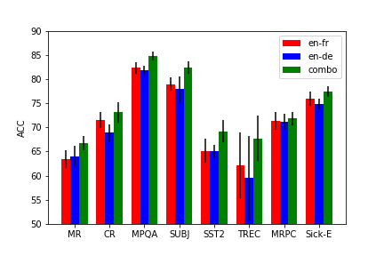
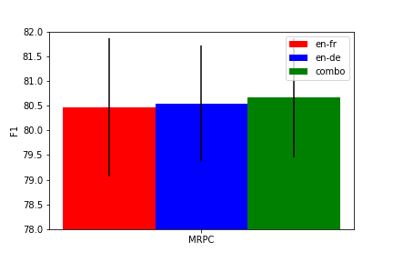
Figure 2: Mean and two standard deviations (error bars) for 10 runs of EmbedAlign on the sentence evaluation benchmarks.

Appendix B Architecture

Figure 3 shows the architecture for the inference and generative models in EmbedAlign, with BiRNN encoder ($h$).

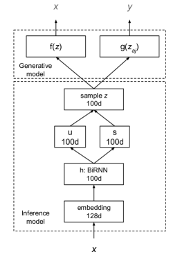
Figure 3: Architecture for EmbedAlign.

References

- AP et al. (2014) Sarath Chandar AP, Stanislas Lauly, Hugo Larochelle, Mitesh Khapra, Balaraman Ravindran, Vikas C Raykar, and Amrita Saha. 2014. An autoencoder approach to learning bilingual word representations. In Advances in Neural Information Processing Systems. pages 1853–1861.
- Bannard and Callison-Burch (2005) Colin Bannard and Chris Callison-Burch. 2005. Paraphrasing with bilingual parallel corpora. In Proceedings of the 43rd Annual Meeting on Association for Computational Linguistics. Association for Computational Linguistics, Stroudsburg, PA, USA, ACL ’05, pages 597–604. https://doi.org/10.3115/1219840.1219914.
- Baydin et al. (2015) Atilim Gunes Baydin, Barak A Pearlmutter, Alexey Andreyevich Radul, and Jeffrey Mark Siskind. 2015. Automatic differentiation in machine learning: a survey. arXiv preprint arXiv:1502.05767 .
- Bojar et al. (2014) Ondrej Bojar, Christian Buck, Christian Federmann, Barry Haddow, Philipp Koehn, Johannes Leveling, Christof Monz, Pavel Pecina, Matt Post, Herve Saint-Amand, Radu Soricut, Lucia Specia, and Aleš Tamchyna. 2014. Findings of the 2014 workshop on statistical machine translation. In Proceedings of the Ninth Workshop on Statistical Machine Translation. Association for Computational Linguistics, Baltimore, Maryland, USA, pages 12–58. http://www.aclweb.org/anthology/W/W14/W14-3302.
- Botev et al. (2017) Aleksandar Botev, Bowen Zheng, and David Barber. 2017. Complementary sum sampling for likelihood approximation in large scale classification. In Artificial Intelligence and Statistics. pages 1030–1038.
- Bowman et al. (2015) Samuel R. Bowman, Gabor Angeli, Christopher Potts, and Christopher D. Manning. 2015. A large annotated corpus for learning natural language inference. In Proceedings of the 2015 Conference on Empirical Methods in Natural Language Processing. Association for Computational Linguistics, Lisbon, Portugal, pages 632–642. http://aclweb.org/anthology/D15-1075.
- Bowman et al. (2016) Samuel R. Bowman, Luke Vilnis, Oriol Vinyals, Andrew M. Dai, Rafal Józefowicz, and Samy Bengio. 2016. Generating sentences from a continuous space. In Proceedings of the 20th SIGNLL Conference on Computational Natural Language Learning, CoNLL 2016, Berlin, Germany, August 11-12, 2016. pages 10–21.
- Brazinskas et al. (2017) Arthur Brazinskas, Serhii Havrylov, and Ivan Titov. 2017. Embedding words as distributions with a bayesian skip-gram model. Arxiv: 1711.11027 .
- Brown et al. (1993) Peter F. Brown, Vincent J. Della Pietra, Stephen A. Della Pietra, and Robert L. Mercer. 1993. The mathematics of statistical machine translation: parameter estimation. Computational Linguistics 19(2):263–311.
- Collobert et al. (2011) Ronan Collobert, Jason Weston, Léon Bottou, Michael Karlen, Koray Kavukcuoglu, and Pavel Kuksa. 2011. Natural language processing (almost) from scratch. J. Mach. Learn. Res. 12:2493–2537. http://dl.acm.org/citation.cfm?id=1953048.2078186.
- Conneau et al. (2017) Alexis Conneau, Douwe Kiela, Holger Schwenk, Loic Barrault, and Antoine Bordes. 2017. Supervised learning of universal sentence representations from natural language inference data. arXiv preprint arXiv:1705.02364 .
- Diab and Resnik (2002) Mona Diab and Philip Resnik. 2002. An unsupervised method for word sense tagging using parallel corpora. In Proceedings of 40th Annual Meeting of the Association for Computational Linguistics. Association for Computational Linguistics, Philadelphia, Pennsylvania, USA, pages 255–262. https://doi.org/10.3115/1073083.1073126.
- Faruqui and Dyer (2014a) Manaal Faruqui and Chris Dyer. 2014a. Community evaluation and exchange of word vectors at wordvectors.org. In Proceedings of the 52nd Annual Meeting of the Association for Computational Linguistics: System Demonstrations. Association for Computational Linguistics, Baltimore, USA.
- Faruqui and Dyer (2014b) Manaal Faruqui and Chris Dyer. 2014b. Improving vector space word representations using multilingual correlation. In Proceedings of the 14th Conference of the European Chapter of the Association for Computational Linguistics. Association for Computational Linguistics, Gothenburg, Sweden, pages 462–471. http://www.aclweb.org/anthology/E14-1049.
- Ferraresi et al. (2008) Adriano Ferraresi, Eros Zanchetta, Marco Baroni, and Silvia Bernardini. 2008. Introducing and evaluating ukwac, a very large web-derived corpus of english. In In Proceedings of the 4th Web as Corpus Workshop (WAC-4.
- Firth (1957) J. R. Firth. 1957. A synopsis of linguistic theory 1930-1955. Studies in Linguistic Analysis pages 1–32.
- Glorot and Bengio (2010) Xavier Glorot and Yoshua Bengio. 2010. Understanding the difficulty of training deep feedforward neural networks. In Yee Whye Teh and Mike Titterington, editors, Proceedings of the Thirteenth International Conference on Artificial Intelligence and Statistics. PMLR, Chia Laguna Resort, Sardinia, Italy, volume 9 of Proceedings of Machine Learning Research, pages 249–256. http://proceedings.mlr.press/v9/glorot10a.html.
- Gouws et al. (2015) Stephan Gouws, Yoshua Bengio, and Greg Corrado. 2015. Bilbowa: Fast bilingual distributed representations without word alignments. In Francis Bach and David Blei, editors, Proceedings of the 32nd International Conference on Machine Learning. PMLR, Lille, France, volume 37 of Proceedings of Machine Learning Research, pages 748–756. http://proceedings.mlr.press/v37/gouws15.html.
- Harris (1954) Zellig S. Harris. 1954. Distributional structure. Word 10(23):146–162.
- Hermann and Blunsom (2014) Karl Moritz Hermann and Phil Blunsom. 2014. Multilingual models for compositional distributed semantics. In Proceedings of the 52nd Annual Meeting of the Association for Computational Linguistics (Volume 1: Long Papers). Association for Computational Linguistics, Baltimore, Maryland, pages 58–68. http://www.aclweb.org/anthology/P14-1006.
- Hill et al. (2014) Felix Hill, Kyunghyun Cho, Sebastien Jean, Coline Devin, and Yoshua Bengio. 2014. Embedding word similarity with neural machine translation. arXiv preprint arXiv:1412.6448 .
- Hochreiter and Schmidhuber (1997) Sepp Hochreiter and Jürgen Schmidhuber. 1997. Long short-term memory. Neural Comput. 9(8):1735–1780. https://doi.org/10.1162/neco.1997.9.8.1735.
- Jordan et al. (1999) MichaelI. Jordan, Zoubin Ghahramani, TommiS. Jaakkola, and LawrenceK. Saul. 1999. An introduction to variational methods for graphical models. Machine Learning 37(2):183–233.
- Kingma and Ba (2014) Diederik P. Kingma and Jimmy Ba. 2014. Adam: A method for stochastic optimization. CoRR abs/1412.6980.
- Kingma and Welling (2014) Diederik P. Kingma and Max Welling. 2014. Auto-encoding variational bayes. In International Conference on Learning Representations.
- Klementiev et al. (2012) Alexandre Klementiev, Ivan Titov, and Binod Bhattarai. 2012. Inducing crosslingual distributed representations of words. In Proceedings of COLING 2012. The COLING 2012 Organizing Committee, Mumbai, India, pages 1459–1474. http://www.aclweb.org/anthology/C12-1089.
- Koehn (2005) Philipp Koehn. 2005. Europarl: A Parallel Corpus for Statistical Machine Translation. In Conference Proceedings: the tenth Machine Translation Summit. AAMT, AAMT, Phuket, Thailand, pages 79–86. http://mt-archive.info/MTS-2005-Koehn.pdf.
- Koehn et al. (2007) Philipp Koehn, Hieu Hoang, Alexandra Birch, Chris Callison-Burch, Marcello Federico, Nicola Bertoldi, Brooke Cowan, Wade Shen, Christine Moran, Richard Zens, Chris Dyer, Ondřej Bojar, Alexandra Constantin, and Evan Herbst. 2007. Moses: Open source toolkit for statistical machine translation. In Proceedings of the 45th Annual Meeting of the ACL on Interactive Poster and Demonstration Sessions. Association for Computational Linguistics, Stroudsburg, PA, USA, ACL ’07, pages 177–180. http://dl.acm.org/citation.cfm?id=1557769.1557821.
- Kočiský et al. (2014) Tomáš Kočiský, Karl Moritz Hermann, and Phil Blunsom. 2014. Learning Bilingual Word Representations by Marginalizing Alignments. In Proceedings of ACL.
- Levy and Goldberg (2014a) Omer Levy and Yoav Goldberg. 2014a. Dependency-based word embeddings. In Proceedings of the 52nd Annual Meeting of the Association for Computational Linguistics (Volume 2: Short Papers). Association for Computational Linguistics, Baltimore, Maryland, pages 302–308. http://www.aclweb.org/anthology/P14-2050.
- Levy and Goldberg (2014b) Omer Levy and Yoav Goldberg. 2014b. Linguistic regularities in sparse and explicit word representations. In Proceedings of the Eighteenth Conference on Computational Natural Language Learning. Association for Computational Linguistics, Ann Arbor, Michigan, pages 171–180. http://www.aclweb.org/anthology/W14-1618.
- Luong et al. (2015) Thang Luong, Hieu Pham, and Christopher D Manning. 2015. Bilingual word representations with monolingual quality in mind. In Proceedings of the 1st Workshop on Vector Space Modeling for Natural Language Processing. pages 151–159.
- McCarthy and Navigli (2009) Diana McCarthy and Roberto Navigli. 2009. The english lexical substitution task. Language Resources and Evaluation 43(2):139–159.
- Melamud et al. (2015) Oren Melamud, Omer Levy, and Ido Dagan. 2015. A simple word embedding model for lexical substitution. In Proceedings of the 1st Workshop on Vector Space Modeling for Natural Language Processing, VS@NAACL-HLT 2015, June 5, 2015, Denver, Colorado, USA. pages 1–7.
- Mihalcea and Pedersen (2003) Rada Mihalcea and Ted Pedersen. 2003. An evaluation exercise for word alignment. In Proceedings of the HLT-NAACL 2003 Workshop on Building and Using Parallel Texts: Data Driven Machine Translation and Beyond - Volume 3. Association for Computational Linguistics, Stroudsburg, PA, USA, HLT-NAACL-PARALLEL ’03, pages 1–10. https://doi.org/10.3115/1118905.1118906.
- Mikolov et al. (2013) Tomas Mikolov, Ilya Sutskever, Kai Chen, Greg S Corrado, and Jeff Dean. 2013. Distributed representations of words and phrases and their compositionality. In C.J.C. Burges, L. Bottou, M. Welling, Z. Ghahramani, and K.Q. Weinberger, editors, Advances in Neural Information Processing Systems 26, Curran Associates, Inc., pages 3111–3119.
- Och and Ney (2000) Franz Josef Och and Hermann Ney. 2000. Improved statistical alignment models. In 38th Annual Meeting of the Association for Computational Linguistics, Hong Kong, China, October 1-8, 2000..
- Padó and Lapata (2006) Sebastian Padó and Mirella Lapata. 2006. Optimal constituent alignment with edge covers for semantic projection. In Proceedings of the 21st International Conference on Computational Linguistics and 44th Annual Meeting of the Association for Computational Linguistics. Association for Computational Linguistics, Sydney, Australia, pages 1161–1168. https://doi.org/10.3115/1220175.1220321.
- Rezende et al. (2014) Danilo Jimenez Rezende, Shakir Mohamed, and Daan Wierstra. 2014. Stochastic backpropagation and approximate inference in deep generative models. In Proceedings of the 31th International Conference on Machine Learning, ICML 2014, Beijing, China, 21-26 June 2014. pages 1278–1286.
- Robbins and Monro (1951) Herbert Robbins and Sutton Monro. 1951. A stochastic approximation method. The Annals of Mathematical Statistics 22(3):400–407.
- Schulz et al. (2016) Philip Schulz, Wilker Aziz, and Khalil Sima’an. 2016. Word alignment without null words. In Proceedings of the 54th Annual Meeting of the Association for Computational Linguistics (Volume 2: Short Papers). Association for Computational Linguistics, Berlin, Germany, pages 169–174. http://anthology.aclweb.org/P16-2028.
- Socher et al. (2011) Richard Socher, Jeffrey Pennington, Eric H. Huang, Andrew Y. Ng, and Christopher D. Manning. 2011. Semi-supervised recursive autoencoders for predicting sentiment distributions. In Proceedings of the 2011 Conference on Empirical Methods in Natural Language Processing. Association for Computational Linguistics, Edinburgh, Scotland, UK., pages 151–161. http://www.aclweb.org/anthology/D11-1014.
- Titsias and Lázaro-Gredilla (2014) Michalis Titsias and Miguel Lázaro-Gredilla. 2014. Doubly stochastic variational bayes for non-conjugate inference. In Proceedings of the 31st International Conference on Machine Learning (ICML-14). pages 1971–1979.
- Tu et al. (2017) Lifu Tu, Kevin Gimpel, and Karen Livescu. 2017. Learning to embed words in context for syntactic tasks. In Proceedings of the 2nd Workshop on Representation Learning for NLP. Association for Computational Linguistics, Vancouver, Canada, pages 265–275. http://www.aclweb.org/anthology/W17-2632.
- Upadhyay et al. (2016) Shyam Upadhyay, Manaal Faruqui, Chris Dyer, and Dan Roth. 2016. Cross-lingual models of word embeddings: An empirical comparison. In Proceedings of the 54th Annual Meeting of the Association for Computational Linguistics (Volume 1: Long Papers). Association for Computational Linguistics, Berlin, Germany, pages 1661–1670. http://www.aclweb.org/anthology/P16-1157.