Nonlinear spherical perturbations in Quintessence Models of Dark Energy

Abstract

Observations have confirmed the accelerated expansion of the universe. The accelerated expansion can be modelled by invoking a cosmological constant or a dynamical model of dark energy. A key difference between these models is that the equation of state parameter $w$ for dark energy differs from $-1$ in dynamical dark energy (DDE) models. Further, the equation of state parameter is not constant for a general DDE model. Such differences can be probed using the variation of scale factor with time by measuring distances. Another significant difference between the cosmological constant and DDE models is that the latter must cluster. Linear perturbation analysis indicates that perturbations in quintessence models of dark energy do not grow to have a significant amplitude at small length scales. In this paper we study the response of quintessence dark energy to non-linear perturbations in dark matter. We use a fully relativistic model for spherically symmetric perturbations. In this study we focus on thawing models. We find that in response to non-linear perturbations in dark matter, dark energy perturbations grow at a faster rate than expected in linear perturbation theory. We find that dark energy perturbation remains localised and does not diffuse out to larger scales. The dominant drivers of the evolution of dark energy perturbations are the local Hubble flow and a supression of gradients of the scalar field. We also find that the equation of state parameter $w$ changes in response to perturbations in dark matter such that it also becomes a function of position. The variation of $w$ in space is correlated with density contrast for matter. Variation of $w$ and perturbations in dark energy are more pronounced in response to large scale perturbations in matter while the dependence on the amplitude of matter perturbations is much weaker.

1 Introduction

One of the central themes of modern cosmology is the quest for understanding the source of the observed acceleration of the expansion rate of the Universe. Early evidence for an accelerating universe came from clustering of galaxies[1]. There were several independent observations indicating that the density parameter for matter is well below unity[2, 3, 4]. The observations of high redshift supernovae of type Ia ruled out a universe without dark energy[7, 5, 6]. Observations of the cosmic microwave background radiation temperature anisotropies require the total density parameter to be very close to unity[8, 9], thus the universe is a mix of normal matter, radiation, dark matter and dark energy[10]. Latest constraints on dark energy models and some discussion around the origin of these constraints may be found in [11, 12, 13, 14, 15, 17, 16, 18].

A number of theoretical models have been proposed to explain the accelerated expansion of the universe. The simplest model that is consistent with observations is the so called cosmological constant $\Lambda$, this suffers from the problem of fine tuning[19, 20]. A number of dynamical dark energy models like Quintessence, k-essence, chaplygin gas, etc. have been proposed, for an overview see the book Dark Energy: Theory and Observations[21]. There are many models that rely on modified theories of gravity. We refer the readers to recent reviews for more details on models of dark energy and observational constraints[20, 22, 23, 24, 25].

Given the large number of possible explanations, the task is to constrain these using observations and also rule out some possibilities. However, all the models can be tuned to produce almost any specified evolution of the scale factor[26]. Thus it is not possible to distinguish between different classes of models using only the evolution of the scale factor. It has been pointed out that the evolution of perturbations in dark energy may be used to distinguish between different classes of models[27]. Perturbative analysis shows that the growth of perturbations in dark energy at small length scales is strongly suppressed, whereas dark energy perturbations can develop a comparable amplitude to perturbations in matter at very large length scales[56].

In this paper we study the evolution of dark energy perturbations at small scales. Our aim is to study the response of dark energy to non-linear perturbations in matter, and to check whether perturbations in dark energy have any discernible effect on dark matter perturbations. In order to simplify analysis, we restrict ourselves to spherically symmetric perturbations.

The spherical collapse model was introduced by Gunn & Gott[32] where they used it to make a theoretical connection with observational properties of Coma cluster. The spherical collapse model has been used very successfully to understand many aspects of structure formation. A mapping between the linear and non-linear collapse is used in the theory of mass function of collapsed halos and its generalisations. Thus a detailed study of spherical collapse for any dark energy model has many potential applications.

Dynamics in a model with a cosmological constant has been studied by many authors, including studies of spherical collapse[33, 34, 35, 36]. Barrow & Saich [36] generalised the spherical collapse model to include the cosmological constant. In this case the equations can be reduced to quadrature and expressed in terms of elliptic integrals. They found that the presence of dark energy leads to a competition between attractive gravity and repulsive dark energy, and small density perturbations do not collapse. Over densities need to be higher than a threshold if these are to form a collapsed object. Perturbations take longer time to collapse, collapsed perturbations are larger for the given mass and hence have a lower density as compared to perturbations in the Einstein-deSitter model.

In this article we present results from study of spherical collapse in a cosmology with dark energy modeled by a minimally coupled canonical scalar field called ’Quintessence’[37] (also see [23]). While there have been earlier attempts at modelling spherical collapse of matter with Quintessence or other models of dark energy, e.g., see [38, 39, 41, 42, 43, 44, 40, 45, 46, 47, 48, 49, 50, 51], almost all of these employ either some perturbative approximation scheme, or make a strong assumption about quintessence field like non-clustering, zero speed of sound, etc. In this study, we do not make any assumption/approximation for field or metric apart from spherical symmetry. We consider fully non-linear, relativistic dynamics of space-time, matter and scalar field. In §2, we introduce the formalism and equations. Initial conditions are presented in §2.0.1, while virialisation conditions and approach after virialisation is described in §2.1. The discussion of results (§3) is organized as follows: §3.1 deals with dark matter perturbations, whereas dark energy/scalar field perturbation are discussed in §3.2. Finally we highlight important results along with a discussion of their implications in §4.

2 Spherical Collapse

In this section we outline our model in terms of equations. The spherical collapse of non-relativistic matter, aka dust can be studied using a metric with spherical symmetry. In case of a universe with any combination of matter, curvature and dust, it can be shown that the Newtonian limit is exact. We are dealing with non-relativistic matter and a scalar field, and in this case there is no appropriate Newtonian limit. Hence we have to work with a fully relativistic model in order to provide a self consistent treatment for the combination of dust and the scalar field.

For modelling spatially isotropic perturbations, we start by considering a general spatially isotropic metric in comoving frame[52, 53]:

$$ds^{2}\,=\,-e^{(2B)}dr^{2}-R^{2}(d\theta^{2}+sin^{2}\theta d\phi^{2})+dt^{2}$$ (2.1)

where $B(t,r)$ and $R(t,r)$ are arbitrary functions of $r$ and $t$. Some of the characteristics of the metric in presence of pressure are discussed by Lynden-Bell, D. and Bičák, J.[54]. We have to solve for these two functions by solving the Einstein’s equations along with field equations and equations governing the evolution of matter density. The full set of equations is as follows:

$$\ddot{B} = -c^{2}e^{-2B}\frac{R^{\prime 2}}{R^{2}}+\frac{c^{2}}{R^{2}}+\frac{\dot{R}^{2}}{R^{2}}-\dot{B}^{2}-4\pi G\rho-\frac{8\pi G}{c}\left[\frac{\dot{\psi}^{2}}{2c^{2}}-e^{-2B}\frac{\psi^{\prime 2}}{2}\right]$$ (2.2)

$$\frac{\ddot{R}}{R} = -\frac{4\pi G}{c}\left[\frac{\dot{\psi}^{2}}{2c^{2}}+\frac{e^{-2B}\psi^{\prime 2}}{2}-V\right]-\frac{1}{2}\frac{\dot{R}^{2}}{R^{2}}+\frac{c^{2}}{2}\left[e^{-2B}\frac{R^{\prime 2}}{R^{2}}-\frac{1}{R^{2}}\right]$$ (2.3)

$$\ddot{\psi} = c^{2}\left[-\frac{\partial V}{\partial\psi}+e^{-2B}\left\{\psi^{{}^{\prime\prime}}-\left(B^{\prime}-\frac{2R^{\prime}}{R}\right)\psi^{\prime}\right\}\right]-\left(\dot{B}+\frac{2\dot{R}}{R}\right)\dot{\psi}$$ (2.4)

$$\dot{\rho_{m}} = -\left(\dot{B}+\frac{2\dot{R}}{R}\right)\rho_{m}$$ (2.5)

Here a dash represents a partial derivative with respect to $r$ and a dot represents a partial derivative with respect to $t$. In this problem, these are the two independent variables. In the present study we work with two potentials($V\propto\psi^{2}$ and $V\propto\exp(-\psi)$).

The structure of the equations is amenable to defining the initial conditions for the variables $B$, $R$, $\dot{B}$, $\dot{R}$, $\rho_{m}$, $\phi$ and $\dot{\phi}$ at all $r$ and then evolving the system. We use a RK-4 based numerical scheme to solve these equations. See Appendix C for details.

2.0.1 Initial conditions

We first solve the equations in absence of any perturbations. In this case there is no dependence on $r$ and the system is identical to a FLRW universe[28, 29, 30, 31]. In the FLRW limit $B(t,r)\rightarrow log(a(t))$ and $R(r,t)\rightarrow a(t)r$. We require the universe to have $30\%$ dust or non-relativistic matter, and $70\%$ dark energy at the present epoch. The latter is contributed by the scalar field. Further, we require $w$, the effective equation of state to be close to $-1$. We also use an additional assumption that $\dot{\psi}=0$ at the initial time. These requirements allow us to fix all unknown parameters related to the scalar field. We set the initial conditions at $z\sim 1000$.

We first solve for evolution of the scale factor. We start the field with zero kinetic energy, i.e., $w=-1$. We see that for both potentials being considered here, we can get solutions where the equation of state parameter stays fairly close to $w=-1$ up to the present time. We have shown the evolution of $w$ and the density parameter for matter ($\Omega_{nr}$) and field ($\Omega_{\psi}$) in figure 1. This exercise allows us to set the parameters of the scalar field at the initial time for the case where we study non-linear evolution of perturbations.

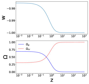
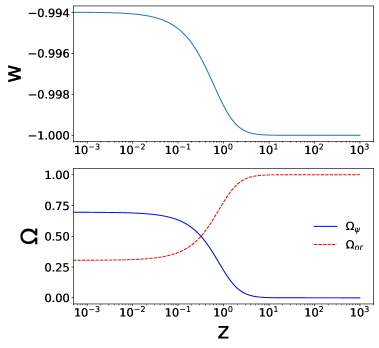
Figure 1: Evolution of the model without any perturbations. This is shown for the two potentials: $V\propto\psi^{2}$ (left column) and $V\propto\exp(-\psi)$ (right column). The top row shows the evolution of the equation of state parameter $w$ as a function of redshift $z$. The lower row shows the evolution of the density parameter for non-relativistic matter and the dark energy components. We use initial conditions for the scalar field used here in all the simulations presented here unless mentioned otherwise. Initial conditions for dark matter at large $r$ also fall back to this set.

We set the initial conditions for the case with perturbations at $z\sim 10^{3}$. We assume that the scalar field representing dark energy is uniform at this time. This has been shown to lead to the expected adiabatic mode for quintessence models [56]. This has also been noted by other authors who have studied attractors for dark energy perturbations [43]. We study results of our calculations at late times, $z\leq 10$ and hence there is adequate time for the solution to approach the attractor. As mentioned above, the scalar field initial conditions are set by assuming that there are no perturbations and we start with $w=-1$:

$$\psi_{i}^{\prime} = 0=\psi_{i}^{\prime\prime}$$

$$\dot{\psi}_{i} = 0$$

$$\psi_{i} = 1$$ (2.6)

Functional form of potentials have some parameters like amplitude of potential $V_{0}$ and $\lambda$ in $V=V_{0}\exp(-\lambda\psi)$. These parameters and initial values are chosen to get the desired background evolution.

The matter distribution has a small initial perturbation. The profile of matter perturbation is compensated, i.e, the central perturbation is offset by a perturbation of opposite sign so that at large $r$, the net perturbation integrated over volume goes to zero. We use the following functional form:

$$\delta_{i}(r)=\left\{\begin{array}[]{lll}\alpha_{0}\left[1-\left(\frac{r}{\sigma_{0}}\right)^{2}\right]^{2}-\alpha_{1}\left[1-\left(\frac{r}{\sigma_{1}}\right)^{2}\right]^{2}&}{&\left(r\leq\sigma_{0}\right)\\ -\alpha_{1}\left[1-\left(\frac{r}{\sigma_{1}}\right)^{2}\right]^{2}&}{&\left(\sigma_{0}<r\leq\sigma_{1}\right)\\ 0&}{&\left(r>\sigma_{1}\right)\\ \end{array}\right.$$ (2.7)

Here we require $\sigma_{0}<\sigma_{1}$. The requirement of net perturbation after averaging over volume to $r=\sigma_{1}$ can be stated as:

$$\int\limits_{0}^{\sigma_{1}}\delta_{i}(r)r^{2}dr=0$$ (2.8)

Thus there is no net perturbation at scales larger than $\sigma_{1}$ and these regions should evolve as a smooth universe. This leads to the following relation between $\alpha_{0}$ and $\alpha_{1}$:

$$\alpha_{1}=\alpha_{0}\left(\frac{\sigma_{0}}{\sigma_{1}}\right)^{3}$$ (2.9)

We set initial velocity of each shell by assuming that these are comoving with the uniform Hubble expansion. This facilitates comparison as this assumption has been used in earlier studies [36] [32] as well. In comparison with linear theory it is important to recall that only $3/5$ of the initial density perturbation in such a case is in the growing mode. Using this with initial condition $R_{i}=a_{i}r$, we can obtain initial conditions for metric coefficients and their time derivatives. For numerical convenience, we redefine the time variable as $t\rightarrow tH_{i}$ where $H_{i}$ is initial value of the Hubble parameter.

$$B_{i} = \ln(a_{i})-\frac{1}{2}\ln\left[1-\frac{3}{r}\frac{\Omega_{im}a_{i}^{2}}{c^{2}}\int drr^{2}\delta(r)\right]$$ (2.10)

$$\dot{B}_{i} = 1$$ (2.11)

$$R_{i} = a_{i}r$$ (2.12)

$${\dot{R}}_{i} = R_{i}$$ (2.13)

$$R^{\prime} = a_{i}$$ (2.14)

$$R^{\prime\prime} = 0$$ (2.15)

The subscript $i$ refers to the initial value of the variable, $a$ is the scale factor and $H$ is the Hubble parameter. $\Omega_{im}$ is the initial value of density parameter for matter.

The argument of the logarithm in the second term in the expression for $B_{i}$ must be positive and hence there is a restriction of the amplitude and scale of perturbations we can simulate. In particular this affects simulations of large scale over densities: comoving initial conditions for arbitrarily large perturbations are not allowed.

The generic solution for a shell with over density is that it expands with the universe at early times. The expansion rate slows down as the gravitational pull of excess mass leads to a more rapid deceleration. The shell reaches a maximum radius, also known as turn around. This is followed by a collapsing phase where the shell falls towards the centre.

2.1 Virialisation and beyond

Mathematical solutions to general spherical collapse lead to formation of a singularity as each shell with a sufficiently high over density collapses to the origin. In a realistic scenario, velocity dispersion as well as non-radial motions that are negligible in the early phase dominate at late times. It is also expected that violent relaxation will drive the system towards virial equilibrium. These are expected to play an important role for dark matter as it cannot radiate or loose energy via any other channel. We proceed with a simplistic approach assuming that in-falling perturbation stabilizes at radius where kinetic energy and potential energy satisfy virial theorem (2.17). In case of Einstein-deSitter universe, this leads to a simple expression for the virial radius: the radius of the virialised halo is exactly half of the maximum or the turn around radius for the shell [32]. Barrow and Saich[36] generalised this to the case when a non-zero cosmological constant is present besides non-relativistic matter.

$$\begin{split}R_{V}=&\left(\frac{2}{3}\right)^{1/3}\left(\frac{\Omega_{\Lambda}R_{T}^{3}+\Omega_{M}(\frac{a_{0}}{a_{in}})^{3}(1+\delta_{in})R_{in}^{3}}{\Omega_{\Lambda}R_{T}}\right)^{1/2}\\ &\sin\left[\frac{1}{3}\arcsin\left\{\frac{\Omega_{M}a_{0}^{3}(1+\delta_{in})R_{in}^{3}}{a_{in}^{3}R_{T}^{3}}\left(\frac{1.5}{1+\frac{\Omega_{M}}{\Omega_{\Lambda}}(\frac{a_{0}R_{in}}{a_{in}R_{T}})^{3}(1+\delta_{in})}\right)^{3/2}\right\}\right]\end{split}$$ (2.16)

Here, $R_{in}$ is the initial radius, $R_{T}$ is the maximum or the turn around radius, $\delta_{in}$ is the initial density contrast inside the shell, $a_{in}$ is the initial value of the scale factor and $a_{0}$ is its present value, $\Omega_{\Lambda}$ is the density parameter corresponding to the cosmological constant at present and $\Omega_{M}$ is the density parameter for non-relativistic matter.

Calculations are much harder in the case of dynamical dark energy. Maor and Lahav [55] summarize two limiting cases for a fluid model of dark energy. They point out that there are significant differences that arise depending upon whether or not dark energy participates in the virialisation process. The two limiting cases they consider are: only dark matter virialises and dark energy does not cluster, and, both dark matter and dark energy virialise. Maor and Lahav [55] show that if only dark matter virialises, then the ratio of virial radius to turn around radius is on lower side of Einstein-DeSitter value of $0.5$, while if the two component system of dark energy plus dark matter virialises together, then this ratio is larger than half. It is relevant to note here that in the case of a cosmological constant, the expected ratio of virial radius to turn around radius is less than half.

As we shall see below, we find that in the case of scalar field, the ratio of virial radius to the turn around radius is less than half.

2.1.1 Evolution of dark energy beyond virialisation

We use the Virialisation condition:

$$<T>+\frac{1}{2}\left\langle R\,F_{R}\right\rangle=0$$ (2.17)

here $T$ is the kinetic energy, $R$ is the radius of the shell and $F_{R}$ is the radial force on the shell. Angular brackets denote averaging over time.

$$T=\frac{1}{2}\dot{R}^{2}\quad F_{R}=\ddot{R}$$ (2.18)

In case of cosmological constant one can use this relation to get an analytical form (2.16) for $R_{V}$ is terms of $R_{T}$ [36]. In case of quintessence being considered here, we track the value of the right hand side of Eqn.2.17 after turn around and declare the shell to have virialised when this value becomes zero for the first time.

It is pertinent to note that this implicitly takes the time of virialisation to be the time when the shell reaches virial radius during the collapsing phase. This is different from the usual interpretation where it is assumed that virialisation happens at the time when the shell collapses to the origin. An implication of this is that the density contrast at the time of virialisation computed here is lower than that obtained with the usual method as the background density is higher. For reference, note that in case of an Einstein-deSitter background, the density contrast at virialisation with this approach is $145$, as compared to $168$ that we obtain using the usual method.

After turn around, we check for condition (2.17) and at that particular $R(r)$ we freeze the metric terms $B(t,r)$ and $R(t,r)$, and we do so because $R(t,r)$ has physical meaning of physical radius which stabilizes at virialisation. In case of $B(t,r)$ we take a cue from $\Lambda CDM$ where $B(t,r)$ is dependent on spatial derivatives of $R(t,r)$. Further, consistency requires that we set time derivatives of the two variables to zero.

As we freeze the metric coefficients, the set of equations we have can no longer be evolved self consistently. Therefore the solutions at later times, after virialisation of the innermost shells, are approximate solutions. As we shall see, dark matter dominates over dark energy in the virialised region and hence an approximate solution can be attempted without expecting a significant back reaction and an implied variation of metric coefficients. The scalar field equations need to be solved over the entire range of scales and it is not obvious whether any choices we make for the solution in the interior of the virialised region will have an impact on the evolution of the field at large scales.

We try three approaches to approximate solution for the scalar field in the virialised region.

1. The scalar field can be evolved as a test field in the space-time determined by the frozen metric coefficients in the virialised region.

2. The scalar field can also be frozen in the virialised region, i.e., we put $\dot{\psi}=0=\ddot{\psi}$ in this region.

3. We put $\ddot{\psi}=0$ and freeze the value of $\dot{\psi}(r)$ inside the virial region.

We compare the three approaches and show that these lead to similar evolution at scales around the virial radius. Further, we show that the solutions are indistinguishable at scales larger than the turn around radius.

In the first approach given above, we solve for the scalar field inside the virial radius according to the following equation:

$$\ddot{\psi}=c^{2}\left[-\frac{\partial V}{\partial\psi}+e^{-2B_{vir}}\left\{\psi^{{}^{\prime\prime}}-\left(B^{\prime}_{vir}-\frac{2R^{\prime}_{vir}}{R_{vir}}\right)\psi^{\prime}\right\}\right]$$ (2.19)

Here, $R_{vir}$ and $B_{vir}$ are the frozen values of metric coefficients inside the virial radius. We solve the full set of equations outside the virial radius.

A comparison of the three approaches is shown in Figure 2. We have plotted the density contrast $\delta_{de}$ for dark energy (top panel) and the equation of state parameter $w$ (lower panel) as a function of scale $r$. The two columns are for two different potentials: the left column is for $V\propto\psi^{2}$ whereas the right column is for $V\propto\exp\left[-\psi\right]$. We have marked the turn around radius with a vertical line on these plots. We find that the qualitative trend is the same for the three approaches. The three approaches have differences at scales close to the virial radius, however the differences decrease rapidly beyond the turn around scale. Percentage difference among three approaches outside virial radius is less than $1\%$ at all scales. The approach where we set $\dot{\psi}=0$ deviates most from the other two approaches and the differences are most obvious in the plot of $w$ as a function of scale $r$.

We use the first approach where the scalar field is evolved as a test field in the fixed background inside the virial radius in the following discussion.

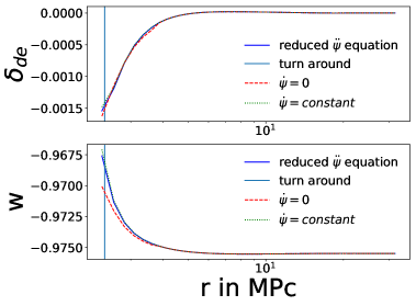
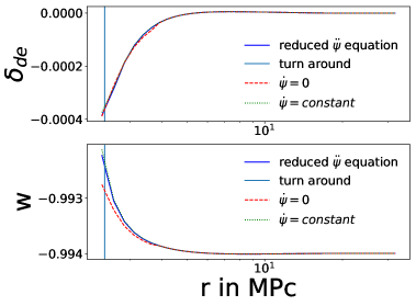
Figure 2: A comparison of the three approaches for evolving the scalar field in the virialised region. Here we show $\delta_{de}$ and $w$ as a function of $r$ at scales outside the virial radius at the present epoch. The left column is for $V\propto\psi^{2}$ and the right column is for $V\propto\exp(-\psi)$ The turn around radius is marked by the vertical line. The amplitude of perturbations is adjusted so that the innermost shells virialise at $z\simeq 1.5$. Simulation OD1 was used for these plots. We find that the three approaches match very well at all scales away from the virial radius. Differences between the three approaches are less than a few percent at all scales, and less than a percent at all scales larger than twice the virial radius.

Simulation	$\sigma_{0}$	$\sigma_{1}$	$\alpha_{0}$	$z_{vir}$
OD1	3	18	0.0068	1.5
OD2	3	18	0.0136	4.0
OD3	6	18	0.0068	1.5
UD1	150	250	-0.0136	-
UD2	20	200	-0.0068	-
UD3	40	200	-0.0068	-
UD4	20	200	-0.0136	-
UD5	100	200	-0.0136	-

Table 1: Parameters used in simulations in this work. Note that for simplicity we have stated the approximate value of the redshift at which the first shell virialises in the case of simulations with over-densities. The simulations are referred to by the Simulation code in figure captions.

3 Results

In this section we present the results of our analysis of the system of spherically symmetric perturbations in dark matter and dark energy. The complete list of simulations with the relevant parameters is given in table 1. The section is divided into sub-sections where we separately study the effect of dark energy perturbations on collapse of dark matter, evolution of dark energy perturbations: both in the case of over density and an under density, analysis of variations with the scale as well as the amplitude of dark matter perturbations, and, a comparison of the evolution of dark energy perturbations with the linear perturbation theory.

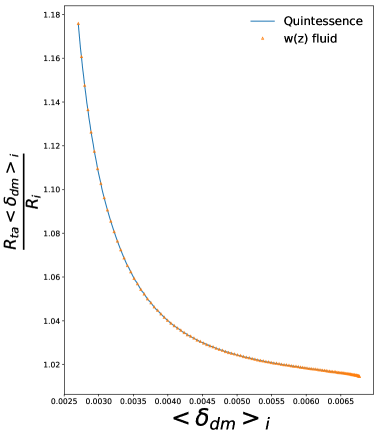
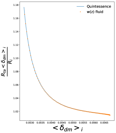
Figure 3: We have plotted the turn around radius in the combination $R_{ta}\langle\delta_{dm}\rangle_{i}/R_{i}$ as a function of the initial density contrast. The expected value of the combination is unity for the Einstein-deSitter model and we see that at large values of $\langle\delta_{dm}\rangle_{i}$ we indeed approach this value. The left panel is for $V\propto\psi^{2}$ while the right panel is for $V\propto\exp(-\psi)$. Simulation OD1 and the same initial conditions for the case without dark energy perturbations have been used for these plots. We plot values from our simulations with perturbations in dark energy as well as from a model where the dark energy does not have any perturbations. The two curves match to better than $0.03\%$ at all scales, indicating that perturbations in dark energy do not influence collapse of dark matter perturbations.

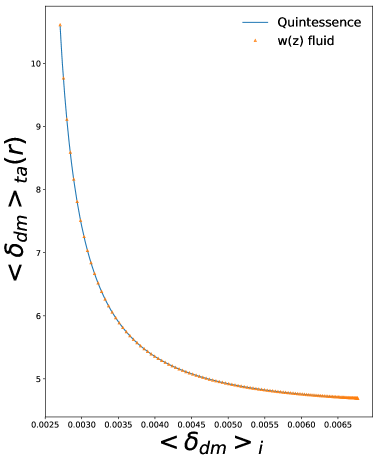
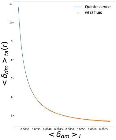
Figure 4: Density contrast at turn around is shown here as a function of the initial density contrast. The expected value of the combination is $4.55$ for the Einstein-deSitter model and we see that at large values of $\langle\delta_{dm}\rangle_{i}$ we indeed approach this value. The left panel is for $V\propto\psi^{2}$ while the right panel is for $V\propto\exp(-\psi)$. We plot values from our simulations with perturbations in dark energy as well as from a model where the dark energy does not have any perturbations. Initial dark matter perturbations here correspond to simulation OD1. The two curves match to better than $0.06\%$ at all scales, indicating that perturbations in dark energy do not influence collapse of dark matter perturbations.

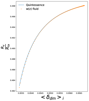
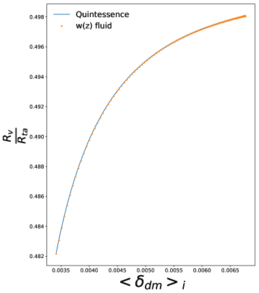
Figure 5: Ratio of virial radius to turn around radius is shown here as a function of the initial density contrast in dark matter. The expected value of the combination is $0.5$ for the Einstein-deSitter model and we see that at large values of $\langle\delta_{dm}\rangle_{i}$ we indeed approach this value. A value lower than $0.5$ signifies that dark energy does not cluster significantly [55]. The left panel is for $V\propto\psi^{2}$ while the right panel is for $V\propto\exp(-\psi)$. We plot values from our simulations (OD1) with perturbations in dark energy as well as from a model where the dark energy does not have any perturbations. The two curves match to better than $0.01\%$ at all scales, indicating that perturbations in dark energy do not influence collapse of dark matter perturbations.

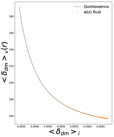
Figure 6: Density contrast at virialisation as a function of the initial density contrast in dark matter. The expected value in our approach for Einstein-deSitter universe is $145$ (see text). We see that the curve is tending towards that value at large initial density contrast. The left panel is for $V\propto\psi^{2}$ while the right panel is for $V\propto\exp(-\psi)$. We plot values from our simulations (OD1) with perturbations in dark energy as well as from a model where the dark energy does not have any perturbations. The two curves match to better than $0.3\%$ at all scales, indicating that perturbations in dark energy do not influence collapse of dark matter perturbations.

3.1 Dark matter perturbations

In order to study the effects of DE perturbations of dark matter, we ran, besides simulations mentioned above, a dark energy model simulation by taking $w(z)$ from the same background and then implementing a non-clustering fluid with same numerical evolution of $w$ to act as DE with following dynamics:

$$\frac{d{\rho_{de}}}{dt}=-3\frac{\dot{a}}{a}(1+w)\rho_{de}$$ (3.1)

Results of a comparative study of this fluid model with full-fledged spherical collapse in quintessence are presented here. We show the comparison for various quantities related to turn around and virialisation. We choose to plot these as a function of the initial density contrast $\delta_{i}$. The choice is motivated by the emergence of a critical value for density contrast required for collapse in the case of the cosmological constant. We find that just like the cosmological constant model for dark energy, there is a critical value that emerges in the dynamical dark energy models. Perturbations with a lower initial density contrast do not enter a collapsing phase. Further, we find that various quantities of interest approach the values obtained in the Einstein-deSitter model as $\delta_{i}$ becomes much larger than the critical value. On the other hand, as we approach the critical initial density contrast from above, dark energy becomes more and more important, and hence it takes longer to begin collapse. Thus the universe expands by a significantly larger amount by the time such perturbations reach turn around or virialisation and hence the average density of matter in the universe is much lower.

Figure 3 shows the turn around radius as a function of $\delta_{i}$. Instead of the turn around radius, we choose to plot the combination $R_{ta}\langle\delta_{i}\rangle/R_{i}$. Here $R_{i}$ is the initial radius of the shell and $\langle\delta_{i}\rangle$ is the average density contrast inside this shell at the initial time. This combination is unity for spherical collapse in the Einstein-deSitter model. The top left panel is for the $\psi^{2}$ potential whereas the top right panel is for the exponential potential. Curve for the model with dark energy perturbations and points for the corresponding model without dark energy perturbations are plotted in the same panels. The difference between the two cases is too small to be seen from these panels. In both models, and for the cases with and without dark energy perturbations, the qualitative trend is the same: the turn around radius is larger for smaller $\delta_{i}$. At large $\delta_{i}$, we approach the turn around radius approaches the expected value in the Einstein-deSitter model. We find that the percentage difference is well below one percent for the turn around radius.

Figure 4 shows the turn around density contrast for different shells in the same format as Figure 3. We find that the density contrast at turn around for shells with large $\delta_{i}$ approaches the expected value for the Einstein-deSitter model. As we approach lower $\delta_{i}$, we find that the density contrast at turn around increases rapidly. This is largely because it takes longer to reach turn around for shells with a smaller initial density contrast, and in this time the density of matter in the universe decreases significantly, leading to a larger density contrast within the perturbation. In this case too, the difference between the model with dark energy clustering and without dark energy clustering is smaller than a percent at all scales for the two potentials studied here.

Figure 5 and Figure 6 show the virial radius (in units of the turn around radius) and the density contrast at the time of virialisation, respectively. We find that the two quantities approach the values expected for the Einstein-deSitter model at large $\delta_{i}$. For shells with smaller $\delta_{i}$, the virial radius is less than half the turn around radius with the ratio decreasing as we get to shells with a smaller initial $\delta_{i}$. The density contrast at virialisation increases rapidly for smaller initial $\delta_{i}$, whereas for larger $\delta_{i}$, we get the value expected in the Einstein-deSitter model ($145$).

3.2 Dark Energy Perturbations

Here we study the evolution of dark energy perturbations in spherical collapse. As stated above, the dark energy component does not have any initial perturbations and therefore perturbations evolve in response to the density contrast in dark matter. The discussion is divided into two segments, one each for an over density in matter, and an under density in matter.

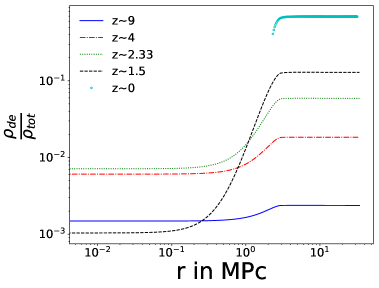
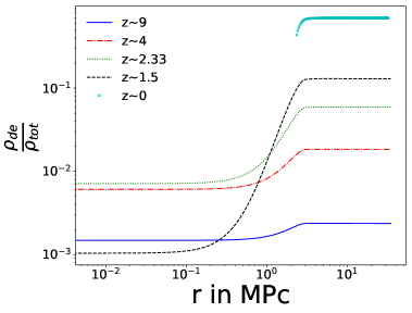
Figure 7: Contribution of Dark Energy to total energy density for over dense case (simulation OD1). We see that at large $r$, the relative contribution of dark energy increases monotonically. However, within the over dense region the contribution of dark energy reaches a maximum of $\sim 0.007$ and then drops to lower values. The left panel is for $V\propto\psi^{2}$ while the right panel is for $V\propto\exp(-\psi)$. We have shown curves outside the virial radius while omitting the values inside the virial radius as we do not have a self-consistent evolution inside the virialised halo. This omission of data within the virial radius impacts only one of the curves shown here.

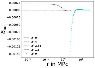
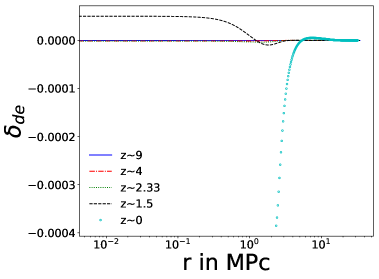
Figure 8: Density contrast for dark energy as a function of scale at different epochs. We see that the amplitude of perturbations in dark energy remains small at all scales and at all times. We have plotted values only at scales outside the virial radius for simulation OD1. The left panel is for $V\propto\psi^{2}$ while the right panel is for $V\propto\exp(-\psi)$.

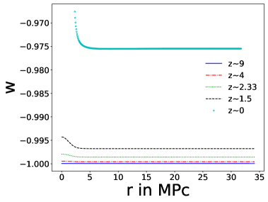
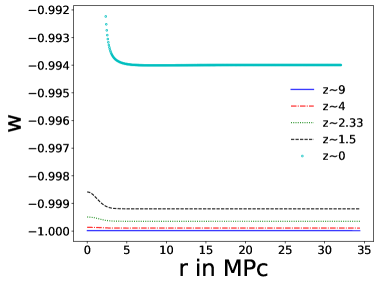
Figure 9: The equation of state parameter for dark energy as a function of scale at different epochs from simulation OD1. We see that the variation in $w$ with scale is fairly significant, particularly at late times. The lower row of plots shows the variation of $w$ with respect to the value in the background model, or the asymptotic value at large scales. We have plotted values only at scales outside the virial radius. The left panel is for $V\propto\psi^{2}$ while the right panel is for $V\propto\exp(-\psi)$.

3.2.1 Over dense Profile

In a region with an initial over density in matter, gravitational instability ensures that the density of dark matter in the region increases monotonically when compared with the average density of matter in the universe. If the initial density contrast is sufficiently high, we find that gravitational instability leads to local collapse and a sharp increase in the density of matter within the collapsed region. It is important to assess the evolution of dark energy density in the region. We show the relative contribution of energy density of dark energy as compared to dark matter drops significantly in the region where dark matter collapses. We show this for a model with $\sigma_{0}=3$ Mpc, $\sigma_{1}=18$ Mpc and the redshift of virialisation $z\sim 1.5$. This is shown in Figure 7 Each curve refers to a specific epoch as marked in the legend. We find that at very large scales dark energy becomes more and more dominant with time, as is expected for the background model that is dominated by dark energy at present. However, within the collapsed region, the relative role of dark energy diminishes strongly at late times. We see that even before virialisation, the energy density of dark energy drops to less than a few percent of its background value near the centre of the perturbation. Thus in terms of the local contribution to the energy budget, dark energy plays a negligible role inside the perturbation.

We plot the density contrast for dark energy as a function of scale for the same model used above. We find that the density contrast for dark energy grows in response to the dark matter perturbation, however its amplitude remains small as compared to unity through the non-linear evolution of dark matter perturbations. Thus we do not expect any significant impact of dark energy density contrast and its variations on observables at small scales.

A surprising feature that may have implications for observations and hence work as a diagnostic for dynamical dark energy models is the spatial variation in the equation of state parameter $w$. We already know from background evolution and our choice of initial conditions that $w=-1$ at early times and it increases slowly with time. We show variation of $w$ as a function of $r$ in Figure 9. This is shown for four epochs leading up to the epoch of virialisation. We find that $w$ increases more rapidly in regions around the collapsing dark matter perturbations.

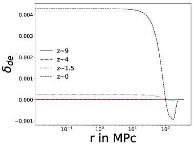
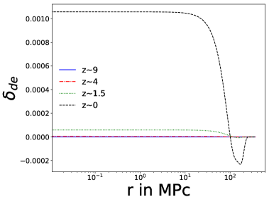
Figure 10: Density contrast for dark energy as a function of scale $r$ for a void, i.e., a matter under-density from simulation UD1. This is plotted at multiple epochs. We find that dark energy perturbations grow but the amplitude remains small in absolute terms. The left panel is for $V\propto\psi^{2}$ while the right panel is for $V\propto\exp(-\psi)$.

Figure 11: Equation of state parameter $w$ as a function of scale $r$ for a void, i.e., a matter under-density for simulation UD1. This is plotted at multiple epochs. We find that $w$ inside the void is smaller than at large scales. The left panel is for $V\propto\psi^{2}$ while the right panel is for $V\propto\exp(-\psi)$.

3.2.2 Under dense Profile

So far we have discussed the evolution of matter over densities. We now turn our attention to the evolution of under densities, or voids. The large scale of voids coupled with the fact that the magnitude of the spatial variation of $w$ is larger for perturbations at large scales makes these a potential test bed for observing the effects of dynamical dark energy.

We show results for a model with $\sigma_{0}=150$ and $\sigma_{1}=250$, thus the characteristic length scale of the perturbation is $250$. We find that the dark energy contributes a very significant fraction to the total energy budget mainly due to depletion of matter. This becomes clear in figure 10 that shows the density contrast in dark energy as a function of scale $r$. We find that the amplitude of density contrast is very small compared to unity at all scales and at all times.

We have plotted the variation of $w$, the equation of state parameter, as a function of scale at different epochs in figure 11. We find that the increase in $w$ with time slows down in under dense regions. This is mainly due to the faster than average expansion rate in the voids. We find that the differential in $w$ is larger for larger voids. The variation with the initial density contrast for matter is less significant, but a larger initial under density leads to a larger differential in $w$.

Voids may be the optimal sites for testing changes in $w$. This is primarily because dark energy dominates in terms of the overall energy budget.

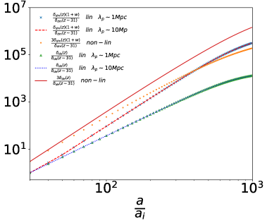
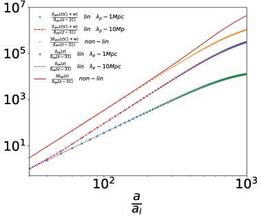
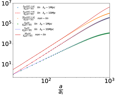
Figure 12: A comparison of the evolution of dark energy perturbations in our simulations UD1 (top panel) and OD1 (lower panel). Left panels are for $V\propto\psi^{2}$ while right one are for $V\propto\exp(-\psi)$. At very large scales the linear theory prediction for the magnitude of dark energy perturbations scales as $(1+w)\delta_{dm}$. We have plotted this combination for linearly evolved $\delta_{dm}$ for two scales: $1$ Mpc (cross) and $10$ Mpc (dashed line). Linear evolution of dark energy density contrast for the two scales is also shown here as triangles ($1$ Mpc) and dotted line ($10$ Mpc). We find that the linear evolution for dark energy perturbations is slower at small scales as compared to the expected variation at large scales. All points pertaining to linear evolution are normalised to unity at the left corner. Also shown in each panel is the combination $\delta_{dm}(1+w)$ at a scale of $6$ Mpc in OD1 and $20$ Mpc in UD1 simulations as small circles. We compare this with the evolution of dark energy density contrast at the same scale in simulations (solid curve). These two sets of points are anchored at $3$ on the left corner: this has been done to facilitate comparison and avoid crowding. We find that the rate of growth of dark energy perturbations in simulations is higher than the linear rate, and also the combination $\delta_{dm}(1+w)$. Thus dark energy perturbations grow at a faster rate in presence of non-linear dark matter perturbations.

3.2.3 Comparison with Linear Perturbation Theory

We have seen that the density contrast in dark energy remains much smaller than unity in all cases considered here. This makes it possible to consider density fluctuations in dark energy at a perturbative level. We compare the rate of growth of dark energy perturbations in our simulations with the rate of growth expected in linear perturbation theory. Such a comparison is useful as it allows us to assess the significance of non-linear dark matter perturbations that our model takes into account.

Before carrying out the comparison, we note that the growth of dark energy perturbations has been studied and it has been found that the growth of perturbations is stunted at small scales. It has been shown that at very large scales $\delta_{DE}\propto(1+w)\delta_{DM}$, which is the expected relation for adiabatic perturbations. For thawing models, $w\simeq-1$ at early times and increases slowly over time. Thus the rate of growth of dark energy perturbations in such models can be much larger than the rate of growth of perturbations of dark matter perturbations. However, same studies indicate that the rate of growth of dark energy perturbations at small scales is slower than the rate at large scales. Specifically, it has been shown that at scales much smaller than the Hubble radius, the linear growth rate is independent of scale.

In figure  12, we show the growth in density contrast for a particular co-moving radius for non-linear spherical case and the corresponding Fourier space amplitude ($\delta_{k}$) for two length scales $1$ Mpc and $10$ Mpc. We show results from two simulations: OD1 (upper panel) and UD1 (lower panel). The curves are normalised at the left corner to avoid crowding and facilitate comparison. This also subsumes an offset required due to different initial conditions (growing mode vs. comoving initial conditions for the two calculations) used in the two different calculations. We find that the rate of growth in the two calculations differs. In particular, at late times, the growth rate of density perturbations in dark energy in the simulation increases and the final amplification factor is more than a factor of ten higher than expected in the linear perturbation theory. In particular, we find that the dark energy density contrast grows faster than the combination $\delta_{dm}(1+w)$ in the simulation whereas the expectation from linear calculation is for a slower growth rate. Thus the non-linear evolution of density fluctuations in dark matter leads to a more rapid growth of perturbations in dark energy.

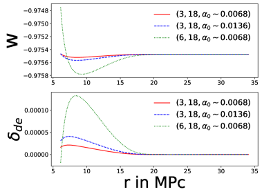
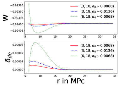
Figure 13: In this figure we explore the dependence of the variation of $w$ on the scale of perturbations in dark matter and also on the amplitude of initial density contrast for dark matter. We plot the variation of $w$ with scale for three models (OD1, OD2 and OD3). Two of the models are for the same initial density contrast in matter but for different scales of perturbation. The third model has the same scale of perturbation as our fiducial model, but has a significantly higher amplitude of the initial matter perturbation. We find that the variation of $w$ is strongest in the model with the larger scale but same amplitude as the fiducial model. The variation with the change in amplitude of perturbation is much smaller. The left panel is for $V\propto\psi^{2}$ while the right panel is for $V\propto\exp(-\psi)$.

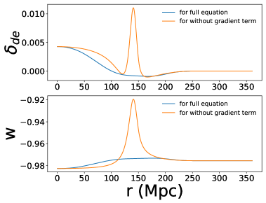
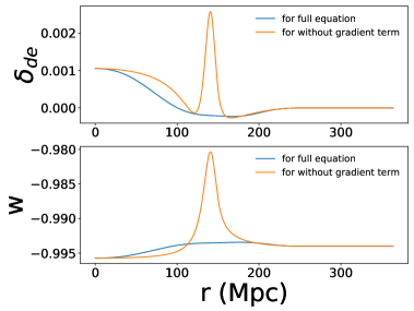
Figure 14: In this figure we explore the leading cause of variation of equation of state parameter $w$ for simulation UD1. We show the variation computed by retaining only the local Hubble expansion terms in the equation of motion and compare it with the full simulation. In the former case, we ignore the gradient term. We find that the variation of $w$ is fairly strong and has some localised features when the gradient terms are ignored. The localised features are not present in the full simulation indicating that the gradients of the scalar field are suppressed in the evolution, and the local Hubble expansion is not the only determining factor.

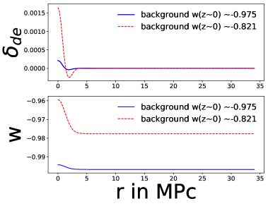
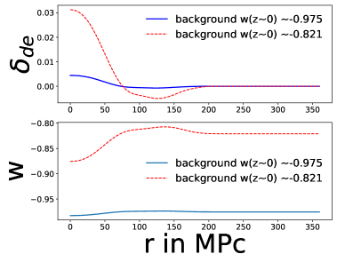
Figure 15: In this figure we study the impact of the equation of state parameter $w$ for the background on the growth of dark energy perturbations and the radial variation of the equation of state parameter. Here we show perturbation growth in two different background models for $V\propto\psi^{2}$. Curves are labeled by present day values of $w$ for the background model. We see that the perturbations have a larger amplitude and $w$ has a larger variation for a larger $1+w_{0}$. The left panel here is for an over-density (OD1) and the right panel is for a void (UD5). We see that the effect is strongly pronounced for under density partly because larger scales are involved. The curves for over density are plotted for $z=1.5$, before virialisation of the innermost shells. Curves for UD5 are plotted at $z=0$.

3.2.4 Exploring dark energy perturbations

The variation in $w$ around a dark matter over density is caused mainly by the slower expansion rate that leads to a more rapid rolling down of the scalar field. In case of under dense regions, the faster expansion slows down the rolling of the field further. We test this conjecture by running a simulation with only the local Hubble flow terms retained. The field equation in this case reduces to:

$$\ddot{\psi}=-c^{2}\frac{\partial V}{\partial\psi}-\left(\dot{B}+\frac{2\dot{R}}{R}\right)\dot{\psi}$$ (3.2)

where we have dropped the terms related to $\psi^{\prime}$ and $\psi^{\prime\prime}$. We find that evolving the system with this equation gives rise to sharp features that are not seen in the full simulation as shown in Figure 14. We surmise that in addition to the variation in expansion rate, there is also a suppression of gradient of the scalar field.

The variation of $w$ around matter perturbations is interesting and we investigate it further. This is important in order to ascertain the possibility of constraining models using observations. Specifically, we explore the magnitude of variation as a function of the amplitude of perturbation, i.e., $\delta_{i}$, and also as a function of the scale of perturbation.

We find that the effect of the scale of perturbation is much more important than the effect of the amplitude of initial perturbation in matter. In Figure 13, we see that for two perturbations with the same amplitude, variation of the scale of perturbation has more pronounced effect than variation of amplitude of perturbation for same scale of perturbation.

We note that we have explored the parameter space for models in the vicinity of the cosmological constant by requiring $w\sim-1$ through the evolution. In models that deviate strongly from the cosmological constant, the perturbations in dark energy become more significant. Example in figure 15 illustrates this where we compare perturbations in models with different present values of the equation of state parameter $w(z=0)$. The amplitude of density contrast in dark energy as well as the radial variation in $w$ is much stronger in the model with the larger $1+w$. We also see that the spatial variation of $w$ for the void is very significant when the present day value for the background deviates strongly from $-1$.

4 Discussion

We have presented results of our analysis of spherical collapse of dark matter and dark energy for a canonical scalar field model. In this section we review these results, discuss the implications and also future directions for our study.

We find that the evolution of dark matter density contrast as well as turn around radius and virialisation are unaffected by dark energy perturbations. This is demonstrated by comparing the evolution in our model with an equivalent model with the same background evolution and no perturbations in dark energy. This result provides justification for ignoring the role of dark energy perturbations while studying collapse of dark matter perturbations. This also implies that there is no significant effect of dark energy perturbations on structure formation. Such effects have been studied earlier in effective models, e.g., [57].

We have shown that the evolution of dark energy perturbations outside the virial radius is insensitive to the scheme used to evolve dark energy perturbations within the virial radius. We have used the approximation of treating the scalar field as a test field inside the virial radius, patching up with the self consistent evolution outside the virial radius. In all plots we have either restricted ourselves to epochs prior to virialisation, or we have plotted functions at scales larger than the virial radius.

We find that the dark energy perturbations remain small, i.e., $|\delta_{DE}|\ll 1$ at all scales and times. This is not to say that there is no effect of non-linear evolution of dark matter perturbations. We show, by comparing with the expected linear growth rate for dark energy perturbations, that the rate of growth of dark energy perturbations is strongly enhanced in the vicinity of non-linear dark matter perturbations. This is encouraging and we plan to study collapse in other dark energy models to explore if dark energy perturbations grow to a significant amplitude in some cases.

This finding encourages us to explore approximations between linear perturbation theory and full non-linear collapse, where we may consider the dark energy to have small perturbations but dark matter may be allowed to have large over densities. It may be possible to relax the restriction of spherical collapse in a suitable approximation scheme.

The most remarkable finding of our work is that the equation of state parameter $w$ becomes a function of space. This has been reported for fluid based models where the equation of state parameter and the effect speed of sound for dark energy perturbations are not the same [58].

The evolution of $w$ in the models being studied here shows a steady increase from the initial value that is close to $-1$ for the background. In the vicinity of over dense regions, this value increases at a faster rate as the local Hubble expansion is slowed down and halted. In voids, the local Hubble expansion is faster than the background and the change in $w$ away from $w=-1$ is slowed down. As a result, $w$ takes on larger values around collapsed halos and it takes on smaller values in voids. Thus $w$ becomes a weak function of over density and we get an interesting coupling between the non-relativistic matter and dark energy sectors even though we are working with a model with minimal coupling.

We find that the effects of dark energy clustering and spatial variation of $w$ are strongest for large scale perturbations. Thus the largest over-densities and voids may be appropriate places to look for observational evidence.

We have considered two thawing models here but we expect that the variation of $w$ will have an opposite trend for freezing models, i.e., it will take on values closer to $-1$ around collapsed halos and values away from this in voids. This expectation follows from the evolution of the field towards the asymptotic value of $-1$, which is slowed down or hastened by the variations in local Hubble flow.

We may model the relation of equation of state parameter as:

$$w\left(\mathbf{r},t\right)=\bar{w}(t)+\epsilon f\left(\delta_{DM},\ldots\right)$$ (4.1)

where $\bar{w}$ is the value for the background model, $\epsilon$ is a small number, and $f$ is a suitable function of density contrast and possibly other quantities such as the velocity field. Such models can be used to explore the impact of spatial variation in $w$ on weak lensing and other physical quantities of interest. It may also be possible to test for such variations by stacking over many objects/voids. We are studying potential avenues for testing the variation of $w$ in space.

We are studying spherical collapse for other models of dark energy. The motivation for these studies is to see whether we can differentiate between such models on the basis of perturbations even if the background evolution is identical. We are aware of the fact that for any given form of the Lagrangian, we can tune the potential to produce a suitable expansion history in the form of an $a(t)$, where $a$ is the scale factor. However, if we fix $a(t)$ then we have precisely one model for each form of Lagrangian. A comparison of perturbations in models with the same expansion history will allow us to explore the information that we may extract from observational probes of perturbations in dark energy.

Appendix A $T^{\mu}_{\nu}$ for scalar field

In order to get Einstein’s equation in the familiar form, we define the stress-energy tensor as follows:

$$T_{\mu\nu}=-2c\left[\frac{\partial L_{\psi}}{\partial g^{\mu\nu}}-\frac{1}{2}L_{\psi}g_{\mu\nu}\right]$$ (A.1)

Owing to spherical symmetry we get the following non-vanishing components.

$$T_{\mu\nu}=c\left[\partial_{\mu}\psi\partial_{\nu}\psi\,-\,L_{\psi}g_{\mu\nu}\right]$$ (A.2)

$$T_{0}^{0}=c\left[\frac{\dot{\psi}^{2}}{2c^{2}}+\frac{e^{-2B}\psi^{\prime 2}}{2}+V\right]$$ (A.3)

$$T_{1}^{1}=-c\left[\frac{\dot{\psi}^{2}}{2c^{2}}+\frac{e^{-2B}\psi^{\prime 2}}{2}-V\right]$$ (A.4)

$$T_{2}^{2}=T_{3}^{3}=-c\left[\frac{\dot{\psi}^{2}}{2c^{2}}-\frac{e^{-2B}\psi^{\prime 2}}{2}-V\right]$$ (A.5)

$$T_{0}^{1}=-ce^{-2B}\dot{\psi}\psi^{\prime}$$ (A.6)

$$T_{1}^{0}=\frac{\dot{\psi}\psi^{\prime}}{c}$$ (A.7)

Vanishing of four divergence of stress energy tensor gives us the equation of motion for the scalar field:

$${T_{0}^{\mu},}_{\mu}=c\dot{\psi}\left[e^{-2B}\left(B^{\prime}\psi^{\prime}-\psi^{\prime\prime}-2\frac{R^{\prime}}{R}\psi^{\prime}\right)+\frac{\dot{B}\dot{\psi}}{c^{2}}+\frac{2\dot{\psi}\dot{R}}{Rc^{2}}+\frac{\ddot{\psi}}{c^{2}}+{V,}_{\psi}\right]=0$$ (A.8)

Appendix B Einstein Equations

Variation of Einstein-Hilbert action gives us:

$$\delta I_{Ein-Hilb}=\frac{c^{3}}{16\pi G}\int{(drd\theta d\phi dt)\sqrt{-g}\left[R_{\mu\nu}-\frac{1}{2}g_{\mu\nu}R_{E}\right]\delta g^{\mu\nu}}$$

where Ricci scalar is represented as $R_{E}$ to distinguish it from metric coefficient $R$. Combining this variation with the stress- energy tensor for $\psi$ in previous sub-subsection, we get Einstein’s equations

$$G^{\mu}_{\nu}=R^{\mu}_{\nu}-\frac{1}{2}\delta^{\mu}_{\nu}R_{E}=\frac{8\pi G}{c^{4}}T^{\mu}_{\nu}$$

$\left({}^{1}_{1}\right)$ component

$$\left[\frac{1}{R^{2}}-e^{-2B}\frac{R^{\prime 2}}{R^{2}}+\frac{\dot{R}^{2}}{c^{2}R^{2}}+\frac{2\ddot{R}}{c^{2}R}\right]=-\frac{8\pi G}{c^{3}}\left[\frac{\dot{\psi}^{2}}{2c^{2}}+\frac{e^{-2B}\psi^{\prime 2}}{2}-V\right]$$ (B.1)

$\left({}^{2}_{2}\right)$ and $\left({}^{3}_{3}\right)$ component

$$e^{-2B}\left[\frac{R^{\prime}B^{\prime}}{R}-\frac{R^{\prime\prime}}{R}\right]+\frac{1}{c^{2}}\left[\frac{\dot{R}\dot{B}}{R}+\frac{\ddot{R}}{R}+\dot{B}^{2}+\ddot{B}\right]=-\frac{8\pi G}{c^{3}}\left[\frac{\dot{\psi}^{2}}{2c^{2}}-\frac{e^{-2B}\psi^{\prime 2}}{2}-V\right]$$ (B.2)

$\left({}^{0}_{0}\right)$ component

$$\begin{split}-e^{-2B}\left[\left(\frac{R^{\prime}}{R}\right)^{2}-\frac{2R^{\prime}B^{\prime}}{R}+\frac{2R^{\prime\prime}}{R}\right]+\frac{1}{R^{2}}+\frac{\dot{R}^{2}}{c^{2}R^{2}}+\frac{2\dot{R}\dot{B}}{c^{2}R}=\\ \frac{8\pi G\rho}{c^{2}}+\frac{8\pi G}{c^{3}}\left[\frac{\dot{\psi}^{2}}{2c^{2}}+\frac{e^{-2B}\psi^{\prime 2}}{2}+V\right]\end{split}$$ (B.3)

$\left({}^{1}_{0}\right)$ and $\left({}^{0}_{1}\right)$ components yield same equation

$$R^{\prime}\dot{B}-\dot{R}^{\prime}=\frac{4\pi G}{c^{3}}\dot{\psi}\psi^{\prime}R$$ (B.4)

Combining equations for $\left({}^{0}_{0}\right)$,$\left({}^{1}_{1}\right)$ and $\left({}^{2}_{2}\right)$ components, we obtain:

$$\ddot{B}=\frac{8\pi G}{c}\left[e^{-2B}\psi^{\prime 2}+V+\frac{\rho c}{2}\right]+2e^{-2B}c^{2}\left[\frac{R^{\prime\prime}}{R}-\frac{R^{\prime}B^{\prime}}{R}\right]-\frac{2\dot{B}\dot{R}}{R}-\dot{B}^{2}$$ (B.5)

or equivalently we can obtain

$$\ddot{B}=-c^{2}e^{-2B}\frac{R^{\prime 2}}{R^{2}}+\frac{c^{2}}{R^{2}}+\frac{\dot{R}^{2}}{R^{2}}-\dot{B}^{2}-4\pi G\rho-\frac{8\pi G}{c}\left[\frac{\dot{\psi}^{2}}{2c^{2}}-e^{-2B}\frac{\psi^{\prime 2}}{2}\right]$$ (B.6)

and from $\left({}^{1}_{1}\right)$, we already have eqn.(B.1). Rewriting it again

$$\frac{\ddot{R}}{R}=-\frac{4\pi G}{c}\left[\frac{\dot{\psi}^{2}}{2c^{2}}+\frac{e^{-2B}\psi^{\prime 2}}{2}-V\right]-\frac{1}{2}\frac{\dot{R}^{2}}{R^{2}}+\frac{c^{2}}{2}\left[e^{-2B}\frac{R^{\prime 2}}{R^{2}}-\frac{1}{R^{2}}\right]$$ (B.7)

Appendix C Numerical Methods

Three second order partial differential equations, eq (2.2),(2.3) and (2.4), can be written as 6 first order partial differential equations and we have two first order partial differential equations for $\rho$ and $R^{\prime}$ giving us total of 8 first order partial differential equations.

$$\dot{x}_{i}(r)=f_{i}\left[x_{1}(r),x_{2}(r),..,x_{8}(r),x^{\prime}_{1}(r),x^{\prime\prime}_{1}(r),x^{\prime}_{3}(r)\right]$$ (C.1)

$$\left\{x_{1},x_{2},x_{3},x_{4},x_{5},x_{6},x_{7},x_{8}\right\}=\left\{\psi,R,B,\dot{\psi},\dot{R},\dot{B},\rho,R^{\prime}\right\}$$ (C.2)

But solving these equations using time ’t’ as parameter turns out to be time consuming, so we switch to background scale factor ’a(t)’ as independent parameter. Switching from ’t’ to ’a’ requires simultaneously solving two more equations for $\dot{a}$ and $\ddot{a}$:

Having structured equations in above form, we used a RK4 algorithm to solve the equations in following flow:

• Initialise all variables

• Loop over ”a” begins

  Calculate spatial derivatives

  RK4 first predictor step to calculate $x_{i}k1$’s

  Calculate spatial derivatives

  RK4 second predictor step to calculate $x_{i}k2$’s

  Calculate spatial derivatives

  RK4 third predictor step to calculate $x_{i}k3$’s

  Calculate spatial derivatives

  RK4 fourth predictor step to calculate $x_{i}k4$’s and correction.

• Loop over ”a” ends

We have tested the algorithm for numerical convergence by varying $\Delta t$ and $\Delta r$. Further, the epoch of virialisation scales correctly with initial density contrasts. We have also solved the equations in the case of $\Lambda$CDM and compared with the solutions obtained using the first integral. These tests have been used to validate the code.

References

- [1] G. Efstathiou, W. J. Sutherland, and S. J. Maddox. The cosmological constant and cold dark matter. Nature, 348:705–707, December 1990.
- [2] S. D. M. White, J. F. Navarro, A. E. Evrard, and C. S. Frenk. The baryon content of galaxy clusters: a challenge to cosmological orthodoxy. Nature, 366:429–433, December 1993.
- [3] J. P. Ostriker and P. J. Steinhardt. The observational case for a low-density Universe with a non-zero cosmological constant. Nature, 377:600–602, October 1995.
- [4] J. S. Bagla, T. Padmanabhan, and J. V. Narlikar. Crisis in Cosmology: Observational Constraints on and H 0. Comments on Astrophysics, 18:275, 1996.
- [5] A. G. Riess, A. V. Filippenko, P. Challis, A. Clocchiatti, A. Diercks, P. M. Garnavich, R. L. Gilliland, C. J. Hogan, S. Jha, R. P. Kirshner, B. Leibundgut, M. M. Phillips, D. Reiss, B. P. Schmidt, R. A. Schommer, R. C. Smith, J. Spyromilio, C. Stubbs, N. B. Suntzeff, and J. Tonry. Observational Evidence from Supernovae for an Accelerating Universe and a Cosmological Constant. AJ, 116:1009–1038, September 1998.
- [6] S. Perlmutter, G. Aldering, G. Goldhaber, R. A. Knop, P. Nugent, P. G. Castro, S. Deustua, S. Fabbro, A. Goobar, D. E. Groom, I. M. Hook, A. G. Kim, M. Y. Kim, J. C. Lee, N. J. Nunes, R. Pain, C. R. Pennypacker, R. Quimby, C. Lidman, R. S. Ellis, M. Irwin, R. G. McMahon, P. Ruiz-Lapuente, N. Walton, B. Schaefer, B. J. Boyle, A. V. Filippenko, T. Matheson, A. S. Fruchter, N. Panagia, H. J. M. Newberg, W. J. Couch, and T. S. C. Project. Measurements of and from 42 High-Redshift Supernovae. ApJ, 517:565–586, June 1999.
- [7] B. P. Schmidt, N. B. Suntzeff, M. M. Phillips, R. A. Schommer, A. Clocchiatti, R. P. Kirshner, P. Garnavich, P. Challis, B. Leibundgut, J. Spyromilio, A. G. Riess, A. V. Filippenko, M. Hamuy, R. C. Smith, C. Hogan, C. Stubbs, A. Diercks, D. Reiss, R. Gilliland, J. Tonry, J. Maza, A. Dressler, J. Walsh, and R. Ciardullo. The High-Z Supernova Search: Measuring Cosmic Deceleration and Global Curvature of the Universe Using Type IA Supernovae. ApJ, 507:46–63, November 1998.
- [8] A. Melchiorri, P. A. R. Ade, P. de Bernardis, J. J. Bock, J. Borrill, A. Boscaleri, B. P. Crill, G. De Troia, P. Farese, P. G. Ferreira, K. Ganga, G. de Gasperis, M. Giacometti, V. V. Hristov, A. H. Jaffe, A. E. Lange, S. Masi, P. D. Mauskopf, L. Miglio, C. B. Netterfield, E. Pascale, F. Piacentini, G. Romeo, J. E. Ruhl, and N. Vittorio. A Measurement of from the North American Test Flight of Boomerang. ApJ, 536:L63–L66, June 2000.
- [9] D. N. Spergel, L. Verde, H. V. Peiris, E. Komatsu, M. R. Nolta, C. L. Bennett, M. Halpern, G. Hinshaw, N. Jarosik, A. Kogut, M. Limon, S. S. Meyer, L. Page, G. S. Tucker, J. L. Weiland, E. Wollack, and E. L. Wright. First-Year Wilkinson Microwave Anisotropy Probe (WMAP) Observations: Determination of Cosmological Parameters. ApJS, 148:175–194, September 2003.
- [10] Planck Collaboration, P. A. R. Ade, N. Aghanim, M. Arnaud, M. Ashdown, J. Aumont, C. Baccigalupi, A. J. Banday, R. B. Barreiro, J. G. Bartlett, and et al. Planck 2015 results. XIII. Cosmological parameters. A&A, 594:A13, September 2016.
- [11] H. K. Jassal, J. S. Bagla, and T. Padmanabhan. Understanding the origin of CMB constraints on dark energy. MNRAS, 405:2639–2650, July 2010.
- [12] E. Piedipalumbo, E. Della Moglie, M. De Laurentis, and P. Scudellaro. High-redshift investigation on the dark energy equation of state. MNRAS, 441:3643–3655, July 2014.
- [13] S. Hotchkiss, S. Nadathur, S. Gottlöber, I. T. Iliev, A. Knebe, W. A. Watson, and G. Yepes. The Jubilee ISW Project - II. Observed and simulated imprints of voids and superclusters on the cosmic microwave background. MNRAS, 446:1321–1334, January 2015.
- [14] D. O. Jones, D. M. Scolnic, A. G. Riess, A. Rest, R. P. Kirshner, E. Berger, R. Kessler, Y.-C. Pan, R. J. Foley, R. Chornock, C. A. Ortega, P. J. Challis, W. S. Burgett, K. C. Chambers, P. W. Draper, H. Flewelling, M. E. Huber, N. Kaiser, R.-P. Kudritzki, N. Metcalfe, J. Tonry, R. J. Wainscoat, C. Waters, E. E. E. Gall, R. Kotak, M. McCrum, S. J. Smartt, and K. W. Smith. Measuring Dark Energy Properties with Photometrically Classified Pan-STARRS Supernovae. II. Cosmological Parameters. ArXiv e-prints, October 2017.
- [15] Gong-Bo Zhao, Marco Raveri, Levon Pogosian, Yuting Wang, Robert G. Crittenden, Will J. Handley, Will J. Percival, Florian Beutler, Jonathan Brinkmann, Chia-Hsun Chuang, Antonio J. Cuesta, Daniel J. Eisenstein, Francisco-Shu Kitaura, Kazuya Koyama, Benjamin L’Huillier, Robert C. Nichol, Matthew M. Pieri, Sergio Rodriguez-Torres, Ashley J. Ross, Graziano Rossi, Ariel G. Sánchez, Arman Shafieloo, Jeremy L. Tinker, Rita Tojeiro, Jose A. Vazquez, and Hanyu Zhang. Dynamical dark energy in light of the latest observations. Nature Astronomy, 8 2017. 27 pages, 3 figures and one table. A supplementary document is included. The BOSS DR12 BAO data used in the work can be downloaded from the SDSS website.
- [16] A. Tripathi, A. Sangwan, and H. K. Jassal. Dark energy equation of state parameter and its evolution at low redshift. J. Cosmology Astropart. Phys., 2017:012, June 2017.
- [17] S. Dhawan, A. Goobar, E. Mörtsell, R. Amanullah and U. Feindt. Narrowing down the possible explanations of cosmic acceleration with geometric probes. J. Cosmology Astropart. Phys., 2017:40, July 2017.
- [18] S. Vagnozzi, S. Dhawan, M. Gerbino, K. Freese, A. Goobar and O. Mena. Constraints on the sum of the neutrino masses in dynamical dark energy models with are tighter than those obtained in CDM. arXiv: 1801.08553, January 2018.
- [19] S. Weinberg. The cosmological constant problem. Reviews of Modern Physics, 61:1–23, January 1989.
- [20] T. Padmanabhan. Dark energy and gravity. General Relativity and Gravitation, 40:529–564, February 2008.
- [21] L. Amendola and S. Tsujikawa. Dark Energy: Theory and Observations. Cambridge University Press, 2010.
- [22] K. Bamba, S. Capozziello, S. Nojiri, S. D. Odintsov Dark energy cosmology: the equivalent description via different theoretical models and cosmography tests. Ap&SS, 342:155-228, November 2012
- [23] S. Tsujikawa. Quintessence: a review. Classical and Quantum Gravity, 30(21):214003, November 2013.
- [24] D. H. Weinberg, M. J. Mortonson, D. J. Eisenstein, C. Hirata, A. G. Riess, and E. Rozo. Observational probes of cosmic acceleration. Phys. Rep., 530:87–255, September 2013.
- [25] D. Huterer and D. L. Shafer. Dark energy two decades after: observables, probes, consistency tests. Reports on Progress in Physics, 81(1):016901, January 2018.
- [26] T. Padmanabhan. Accelerated expansion of the universe driven by tachyonic matter. Phys. Rev. D, 66(2):021301, June 2002.
- [27] H. K. Jassal. Comparison of perturbations in fluid and scalar field models of dark energy. Phys. Rev. D, 79(12):127301, June 2009.
- [28] Friedmann, A.. Über die Krümmung des Raumes. Zeitschrift fur Physik, 10:377-385, 1922.
- [29] Lemaître, G.. Expansion of the universe, A homogeneous universe of constant mass and increasing radius accounting for the radial velocity of extra-galactic nebulae. MNRAS, 91:483-490, March 1931.
- [30] Robertson, H. P.. Kinematics and World-Structure. ApJ, 82:284, Nov.1935.
- [31] Walker A. G.. On Riemannian spaces with spherical symmetry about a line, and the conditions for isotropy in general relativity. The Quarterly Journal of Mathematics, 6:81-93, 1935.
- [32] J. E. Gunn and J. R. Gott, III. On the Infall of Matter Into Clusters of Galaxies and Some Effects on Their Evolution. ApJ, 176:1, August 1972.
- [33] Peebles P. J. E.. Tests of cosmological models constrained by inflation. ApJ, 284:439-444, September 1984.
- [34] Eke V. R., Cole S., Frenk C. S.. Cluster evolution as a diagnostic for Omega. MNRAS, 282:263-280, September 1996.
- [35] Lahav O., Lilje P. B., Primack J. R., Rees M. J.. Dynamical effects of the cosmological constant. MNRAS, 251:128-136, July 1991.
- [36] J. D. Barrow and P. Saich. Growth of large-scale structure with a cosmological constant. MNRAS, 262:717–725, June 1993.
- [37] R. R. Caldwell, R. Dave, and P. J. Steinhardt. Cosmological Imprint of an Energy Component with General Equation of State. Physical Review Letters, 80:1582–1585, February 1998.
- [38] L. R. Abramo, R. C. Batista, L. Liberato and R. Rosenfeld. Structure formation in the presence of dark energy perturbations. J. Cosmology Astropart. Phys., 2007:12, November 2007.
- [39] L. R. Abramo, R. C. Batista, L. Liberato and R. Rosenfeld. Physical approximations for the nonlinear evolution of perturbations in inhomogeneous dark energy scenarios. Phys. Rev. D, 79:023516, January 2009.
- [40] V. Marra and M. Pääkkönen. Exact spherically-symmetric inhomogeneous model with n perfect fluids. J. Cosmology Astropart. Phys., 2012:25, January 2012.
- [41] Z. Roupas, M. Axenides, G. Georgiou and E. N. Saridakis. Galaxy clusters and structure formation in quintessence versus phantom dark energy universe. Phys. Rev. D, 89.083002, April 2014.
- [42] P. Creminelli, G. D’Amico, J. Noreña, L. Senatore, and F. Vernizzi. Spherical collapse in quintessence models with zero speed of sound. J. Cosmology Astropart. Phys., 2010:027, March 2010.
- [43] G. Ballesteros and J. Lesgourgues. Dark energy with non-adiabatic sound speed: initial conditions and detectability. J. Cosmology Astropart. Phys., 2010:014, October 2010.
- [44] S. Anselmi, G. Ballesteros, and M. Pietroni. Non-linear dark energy clustering. J. Cosmology Astropart. Phys., 2011:014, November 2011.
- [45] M. Tsizh and B. Novosyadlyj. Dynamics of dark energy in collapsing halo of dark matter. Advances in Astronomy and Space Physics, 5:51–56, September 2015.
- [46] Christian Fidler, Thomas Tram, Cornelius Rampf, Robert Crittenden, Kazuya Koyama, and David Wands. Relativistic interpretation of newtonian simulations for cosmic structure formation. Journal of Cosmology and Astroparticle Physics, 2016(09):031, 2016.
- [47] J. Rekier, A. Füzfa, and I. Cordero-Carrión. Nonlinear cosmological spherical collapse of quintessence. Phys. Rev. D, 93:043533, Feb 2016.
- [48] D. Herrera, I. Waga, and S. E. Jorás. Calculation of the critical overdensity in the spherical-collapse approximation. Phys. Rev. D, 95:064029, Mar 2017.
- [49] Shuxun Tian, Shuo Cao, and Zong-Hong Zhu. The dynamics of inhomogeneous dark energy. The Astrophysical Journal, 841(1):63, 2017.
- [50] I. Achitouv. Improved model of redshift-space distortions around voids: Application to quintessence dark energy. Phys. Rev. D, 96(8):083506, October 2017.
- [51] C.-C. Chang, W. Lee, and K.-W. Ng. Spherical collapse models with clustered dark energy. Physics of the Dark Universe, 19:12–20, March 2018.
- [52] Tolman, R. C. Effect of Inhomogeneity on Cosmological Models. Proceedings of the National Academy of Science, 20:169–176, March 1934.
- [53] Bondi, H. Spherically symmetrical models in general relativity. MNRAS. 107:410–425, 1947.
- [54] Lynden-Bell, D. and Bičák, J. Pressure in Lemaître-Tolman-Bondi solutions and cosmologies. Classical and Quantum Gravity. 33:075001, April 2016.
- [55] I. Maor and O. Lahav. On virialization with dark energy. J. Cosmology Astropart. Phys., 7:003, July 2005.
- [56] S. Unnikrishnan, H. K. Jassal, and T. R. Seshadri. Scalar field dark energy perturbations and their scale dependence. Phys. Rev. D, 78(12):123504, December 2008.
- [57] R. C. Batista and V. Marra. Clustering dark energy and halo abundances. J. Cosmology Astropart. Phys., 2017:48, November 2017.
- [58] L. R. Abramo, R. C. Batista, L. Liberato and R. Rosenfeld. Dynamical mutation of dark energy. Phys. Rev. D, 77:067301, March 2008.