Abstract

A fast and automated scheme for general polarization transformations holds great value in adaptive optics, quantum information, and virtually all applications involving light-matter and light-light interactions. We present an experiment that uses a liquid crystal on silicon spatial light modulator (LCOS-SLM) to perform polarization transformations on a light field. We experimentally demonstrate the point-by-point conversion of uniformly polarized light fields across the wave front to realize arbitrary, spatially varying polarization states. Additionally, we demonstrate that a light field with an arbitrary spatially varying polarization can be transformed to a spatially invariant (i.e., uniform) polarization.

OCIS codes: (070.6120) Spatial light modulators; (110.1080) Active or adaptive optics; (260.5430) Polarization; (230.3720) Liquid-crystal devices; (270.5585) Quantum information and processing.

1 Introduction

In conventional photonic applications, the polarization state of a light field is often considered to be uniform across the wave front, i.e., the same polarization exists at each position in the field’s transverse profile. Conventional optical elements, such as waveplates, are transversely invariant and, thus, maintain this polarization uniformity. While these uniform polarization transformations have proven useful in a variety of quantum and classical applications such as quantum key distribution (QKD), Stokes polarimetry, and ellipsometry, there has been considerable recent interest in non-uniform polarization structures [1, 2]. In [3], it was shown that radially polarized light fields can be focused to a smaller spot than similar uniformly polarized fields. In telecommunications, spatially distinct regions of the light field can function as independent, polarization-encoded channels. Non-uniform polarization states push the boundaries of polarization imaging [4], where graphical information is encoded in a light field in such a way that is invisible to the naked eye. These nascent applications show that a means of arbitrarily manipulating polarization in full generality has considerable potential in both science and industry. This work demonstrates a method for such manipulation that uses liquid crystal spatial light modulators (SLMs).

Over the past three decades, SLMs have been used to generate light fields with specific intensity and phase profiles [5, 6, 7]. Beginning with some initial work in 2000, a few research groups have also begun producing spatially varying polarization profiles using SLMs. However, the full potential of this approach has yet to be realized. In [8, 9], the set of produced polarization states were limited to those in a plane of the Poincaré sphere. Other previous experiments often suffer from an inherent optical loss due to their diffractive or interferometric design [10, 11, 12, 13, 14, 15, 16, 17, 18]. Unlike in classical imaging or telecommunications, where substantial optical loss can be tolerated, even small loss can stop quantum information and quantum metrology applications from functioning at all. Moreover, quantum applications often require sophisticated state transformations, whereas past work has focused on producing particular non-uniform polarization states [19, 20, 21, 22, 23, 24].

In our demonstration, SLMs are used without any diffractive or interferometric methods to exploit the device’s ability to perform various polarization transformations. Following the proposal in [25], we show that two sequential SLM incidences will induce a controllable, near- arbitrary conversion of the polarization point-by-point across the wave front of a light field. In our demonstration, both incidences are on the same SLM device. While routing the light for this scheme necessitates considerable loss, the setup serves as a proof-of-principle demonstration for a design that has no inherent loss. Specifically, a setup based on two transmissive SLMs will only suffer from loss due to technical issues, such as the SLM array fill-factor or anti-reflection coating performance, both of which can be improved through technical refinements. In summary, we demonstrate the production of sophisticated spatially varying polarization profiles, and, more generally, we show that we can transform polarizations in a similarly sophisticated manner.

We begin in Section 2 by reviewing the theory behind our method, as first described in [25]. The experimental setup is detailed in Section 3. The key to our successful demonstration is a careful procedure, described in Section 4, to calibrate the operation of the device. We present the experimental results in Section 5. There, we demonstrate the production of arbitrary, spatially varying polarization states from a known uniform polarization state. The degree of control and sophistication that we can achieve in our scheme is demonstrated by our ability to paint with polarization: we render Van Gogh’s painting Starry Night in elliptical polarization states. We then demonstrate the scheme’s ability to convert arbitrary input polarizations by homogenizing a beam with dramatic spatial polarization variation. In short, we ‘heal’ the polarization of an aberrated light field.

2 Theory

2.1 Polarization transformations with SLMs

In this work, we restrict ourselves to perfectly polarized fields. These are represented by reduced Stokes vectors $\mathbf{S}=[s_{1},s_{2},s_{3}]$ in the Poincaré sphere (having orthogonal axes $\mathbf{S_{1}},\mathbf{S_{2}},$ and $\mathbf{S_{3}}$) with $\mathbf{\left|S\right|}^{2}=s_{1}^{2}+s_{2}^{2}+s_{3}^{2}=1$. The conventions and notation used for this formalism are identical to those used by Sit et al. and can be found in Appendix A of their work [25]. A general unitary (i.e., lossless and noiseless) polarization transformation is most simply described by a rotation $\hat{R}(\zeta,\mathbf{k})$ of a Stokes vector $\mathbf{S}$ about an axis $\mathbf{k}$ of the Poincaré sphere by an angle $\zeta$ known as the retardance.

The work horse behind polarization transformations in our experiment is the SLM – a spatial array of liquid crystal (LC) cells with a common optical axis. Under standard SLM mounting, this axis is oriented along the horizontal or vertical laboratory direction, which in our convention is along the $\pm\mathbf{S_{1}}$ polarizations. It follows that each cell, labelled by $(i,j)$, in the SLM array induces the rotation $\hat{R}(\zeta_{ij},\mathbf{S_{1}})$, where $\zeta_{ij}$ is set by the birefringence of the cell. In turn, the birefringence of each individual cell can be controlled by an applied voltage. Consequently, distinct transverse positions $(x_{j},y_{i})$ of a light field incident on an SLM can acquire distinct polarizations, thereby creating a spatially non-uniform polarization.

2.2 The two-step scheme

In order to rotate about other axes in the Poincaré sphere without physically rotating the SLM, the SLM can be sandwiched between matched sets of waveplates. In effect, these waveplates rotate the polarization basis in which the SLM acts. For example, if the SLM is preceded by a half waveplate (HWP) with its optic axis oriented at $22.5^{\circ}$ to the horizontal and followed by another HWP at $22.5^{\circ}+90^{\circ}$, then it will effectively rotate the polarization about $\mathbf{S_{2}}$, the diagonal and anti-diagonal polarization axis.

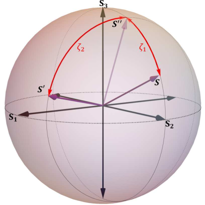
Fig. 1: The two-step scheme. The first step is a rotation in the Poincaré sphere about $\mathbf{S_{1}}$, the second is a rotation about $\mathbf{S_{2}}$. The point at which the first rotation ends and second rotation starts is denoted by $\mathbf{S}"$. This intermediate point is described by Eq. (7) in the appendix.

This second axis comes in to use in the two-step transformation scheme, theoretically described by Sit et al. in [25] and shown in Fig. 1. This scheme is composed of two successive rotations with fixed rotation axes $\mathbf{S_{1}}$ and $\mathbf{S_{2}}$, i.e., $\hat{R}(\zeta_{2,ij},\mathbf{S_{2}})\hat{R}(\zeta_{1,ij},\mathbf{S_{1}})$. It converts an arbitrary input state $\mathbf{S}{}_{ij}=[s_{1,ij},s_{2,ij},s_{3,ij}]$ to any arbitrary output state $\mathbf{S}^{\prime}_{ij}=[s^{\prime}_{1,ij},s^{\prime}_{2,ij},s^{\prime}_{3,ij}]$ with $(s^{\prime}_{2,ij})^{2}\leq 1-(s_{1,ij})^{2}$. The initial Stokes vector is rotated about $\mathbf{S_{1}}$ until the desired $s_{2,ij}$ component of $\mathbf{S}^{\prime}_{ij}$ is reached. Then, this intermediate Stokes vector is rotated about $\mathbf{S_{2}}$ until the desired $s_{1,ij}$ component of $\mathbf{S}^{\prime}_{ij}$ is reached. The sign of the last component $s_{3,ij}$ is set by either the first or second rotation and its magnitude is set by our normalization, $|\mathbf{S}^{\prime}_{ij}|=1$. The exact formulae for the rotation angles $\zeta_{1,ij}$ and $\zeta_{2,ij}$ are non-trivial. They are derived in [25] and given in Appendix A2 for convenience. In our experiment, two successive incidences on a single SLM compose the two steps in the two-step scheme.

While this two-step transformation is, seemingly, almost completely general, it is not. A crucial distinction is that the input and output states must be known a priori since the rotation angles $\zeta_{1,ij}$ and $\zeta_{2,ij}$ depend on them [25]. The output state can be chosen as a target, whereas the input state can either be determined experimentally point-by-point or produced via a trusted procedure (e.g., a polarizer). Consequently, the two-step scheme could not be used to completely compensate for a general unitary polarization transformation, such as those occurring in optical fibres. Any chosen pair of orthogonal states could be compensated, but no others.

Still, the capabilities of the two-step scheme are substantial. For example, as long as the input state $\mathbf{S}{}_{ij}$ has $s_{1,ij}=0$, any output polarization $\mathbf{S}^{\prime}_{ij}$ can be attained. Conversely, any input polarization state can be transformed to any desired $\mathbf{S}^{\prime}_{ij}$ that has $s^{\prime}_{2,ij}=0$.

2.3 Characterizing spatially varying polarizations

To operate and evaluate the two-step scheme, we completely determine the polarization $\mathbf{S}^{\prime}_{ij}$ point-by-point across the output field using Stokes polarimetry (see Section 3 for technical details). In order to visualize the system performance, we will create two dimensional density plots for each of the three Stokes components. While these are a complete characterization of the output field’s polarization, it is more useful to distill relevant characteristics of the $\mathbf{S}{}_{ij}$ matrix into a quantitative performance metric.

First, we identify a spatial region of interest $A$ in the field in which we reduce the $\mathbf{S}{}_{ij}$ matrix to an average Stokes vector given by,

$$\bar{\mathbf{S}}=\frac{\sum_{i,j=1}^{A}\mathbf{S}{}_{ij}}{|\sum_{i,j=1}^{A}\mathbf{S}{}_{ij}|}.$$ (1)

In most measurements, we will be analyzing the full spatial extent of the field. However, we limit the region $A$ to a circle with a diameter equal to the full width at tenth maximum (FWTM) beam waist in order to avoid the noisy signal in regions of vanishing light intensity. In some measurements, we will set $A$ to be a wedge (i.e., circular sector) of this FWTM circle. The wedge is chosen so that it is contained within a chosen spatial quadrant of the beam.

Our first metric is reminiscent of the well-known degree of polarization [26], but is specifically for non-uniformly polarized light fields. We define the uniformity $U$ of the polarization of the light field to be the length of the average Stokes vector,

$$U\equiv\left|\bar{\mathbf{S}}\right|.$$ (2)

The uniformity metric varies from $U=0$ for spatially varying polarizations to $U=1$ for a light field that has the same polarization everywhere in region $A$. For example, if half the region is any particular polarization and the other half is the orthogonal polarization then $U=0$.

Our second metric, fidelity $F,$ parametrizes the similarity of two polarization states,

$$F\left(\bar{\mathbf{S}}_{\mathrm{exp}},\mathbf{S}_{\mathrm{ideal}}\right)\equiv\frac{1}{2}\left(1+\bar{\mathbf{S}}_{\mathrm{exp}}\cdot\mathbf{S}_{\mathrm{ideal}}\right).$$ (3)

The $\cdot$ symbol denotes the standard vector dot product. The average Stokes vector $\bar{\mathbf{S}}_{\mathrm{exp}}$, typically calculated from the output of the experiment, is potentially imperfect in two ways; the direction of the Stokes vector can differ from $\mathbf{S}_{\mathrm{ideal}}$ and it might have a norm of less than one, signifying non-uniformity. In contrast, the ideal state $\mathbf{S}_{\mathrm{ideal}}$, typically the target state, always has a norm of one. This ensures that $F$ matches a well-known measure from quantum information theory known as the Uhlmann fidelity [27]. The fidelity varies from $F=0$, for two orthogonal polarization states, to $F=1$, for two identical polarization states. These two bounds can only be reached when $\bar{\mathbf{S}}_{\mathrm{exp}}$ is uniform, $U=1$.

With these two metrics in hand, we will be able to characterize how well we can produce a target state and the degree to which we can change the spatial variation of polarization across a region $A$.

3 Experimental Setup

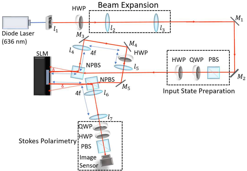
Fig. 2: Schematic of experimental setup (see text for details). The NPBS are tilted by a small angle $\delta$ to ensure that unwanted reflections from the faces of the NPBS are directed away. Lenses $l_{4}-l_{7}$ each have a focal length $f=100mm$. Note: $\textrm{M}_{i}$: mirror, SLM: spatial light modulator, HWP: half waveplate, QWP: quarter waveplate, NPBS: non-polarizing beamsplitter, PBS: polarizing beamsplitter.

Ideally, one would use two transmissive SLMs in sequence to implement the two polarization rotations of the two-step scheme. The only loss would be from non-ideal performance of the optical elements. Currently, however, reflective SLMs have better performance specifications and are more common in optics laboratories. Consequently, we adapt the simple (and ideal) transmissive SLM scheme to reflective SLMs by using 50:50 non-polarizing beamsplitters (NPBS) to separate the incident and reflected light. This has the disadvantage that 50% of the light is lost at each encounter with a NPBS. Since each of the two NPBSs is passed through twice, the total optical transmission is at most 6.25%. Nonetheless, most of the techniques developed here will be applicable in the future to the lossless, transmissive SLM scheme. In this way, it functions as proof-of-principle demonstration and a prototype. Moreover, using a reflective SLM enables us to use the two halves of a single SLM array for the two rotations. A schematic of the setup can be found in Fig. 2.

We begin by describing our source of light and how we produce input polarizations. A continuous wave single-mode fibre-pigtailed diode laser is operated at a sub-threshold bias current in order to achieve a full-width half-maximum spectral bandwidth of 13.2 nm. This is critical for mitigating interference between reflections from, say, the front glass surface and the back silicon surface of the SLM, a topic discussed in [28]. The fibre output is collimated and then expanded by lenses $l_{1},$ $l_{2},$ and $l_{3}$ to have a $1/e^{2}$ beam radius of 1.28 mm. The light then passes through a PBS, QWP, and HWP to generate a well-defined uniform input polarization state. We optionally insert spatially varying birefringent elements here in order to create a non-uniform polarization state.

The light passes through the first 50:50 NPBS and is then incident on the right half of the SLM (Hamamatsu X10468-07, $792\times 600$ pixels, pixel size $20\times 20$ $\mu$m, 256 phase increments) normal to its surface. Here, the first polarization rotation, $\hat{R}(\zeta_{1,ij},\mathbf{S_{1}})$, occurs. The light then reflects from this half of the SLM and the first NPBS and is directed by silver mirrors through a HWP with its optical axis oriented at $22.5^{\circ}$ from the horizontal. The light transmits through a second 50:50 NPBS before its incidence on the left half of the SLM, where a second polarization rotation occurs. When this rotation is considered with the HWP, this rotation is $\hat{R}(\zeta_{2,ij},\mathbf{S_{2}})$. Finally, the light reflects from the SLM and the second NPBS and heads towards the Stokes polarimetry apparatus.

The two-step scheme is capable of tailoring highly non-uniform output polarization profiles. To do so, the SLM must impart a large phase gradient across the light field, which, in turn, creates components of the field travelling at large angles. In order to retain this angular spread, a $4f$ imaging system is used to image the field on each half of the SLM. Each 4f imaging system consists of a pair of lenses ($f=100$ mm, diameter $2.5$ cm, planoconvex) separated by $2f$. The first and last lens are positioned a distance $f$ away from the object and image plane, respectively. The first 4f system ($l_{4},$ $l_{5}$) images the field at the right half of the SLM onto the left half of the SLM. The second $4f$ system ($l_{6},$ $l_{7}$) images the field at the left half of the SLM onto an image sensor. In the appendix, we detail how we compensate for image flips caused by the mirrors and lenses.

Following this last lens, we characterize the output polarization by conducting standard Stokes polarimetry using a QWP, HWP, and PBS [29]. Combined with a digital image sensor (Basler aca1600-20gm, $1626\times 1236$ pixels, pixel size of $4.4\times 4.4$ $\mu$m, 12-bit bit depth, zero gain, 0.65 s exposure), this allows us to measure each Stokes component at each sensor pixel, thereby determining the polarization state point-by-point across the light field. In order to reduce the effect of waveplate retardance errors, we eliminate the second HWP that is nominally required for a rotation about $\mathbf{S_{2}}$. Its absence can be compensated for in the data analysis by simply swapping the definitions of the Stokes components $s_{1}$ and $s_{2}$ with one another. All waveplates are true zero-order with a design wavelength of 633 nm.

4 Experimental Setup Calibration

4.1 SLM Phase-Grey Calibration

The amount of phase that the SLM imparts at a given pixel is directly proportional to an 8-bit value at that pixel. Since the SLM is electronically controlled by a standard digital video signal, we refer to this as a greyscale. The phase to greyscale relationship is nominally given by the manufacturer as a linear function, $\zeta_{ij}\left(g_{ij}\right)=Cg_{ij}$, where $g_{ij}\in[0,255]$ is the greyscale value at pixel $(i,j)$ and $C=2\pi/118$ is the nominal phase-grey proportionality constant provided by the manufacturer. However, we have found that the value of $C$ varies from one pixel to the next, as seen in Fig. 3. To accurately program the SLM, an independent calibration of each illuminated pixel was carried out. This was accomplished by measuring the rotation in polarization at discrete points $(i,j)$ of the output light field as a function of greyscale on the corresponding pixels $(i^{\prime},j^{\prime})$ on the SLM. We used look up tables (LUTs) to define this exact phase-grey relationship $\zeta_{ij}\left(g_{ij}\right)$ for each SLM pixel.

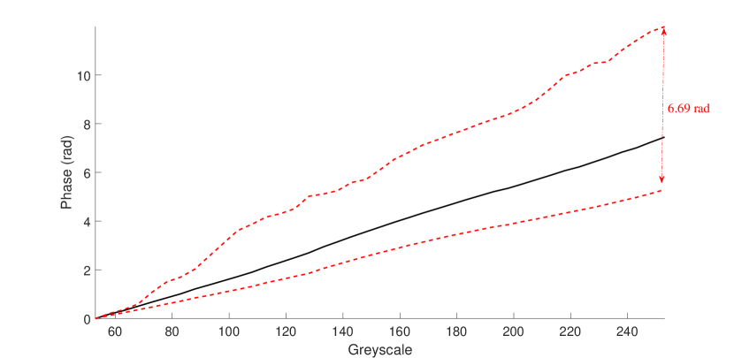
Fig. 3: The phase-grey relationship is plotted for pixels within the $1/e^{2}$ beam waist across the wave front. The red dashed curves correspond to the pixels which had the largest and smallest changes in phase for a change in greyscale, and the black curve denotes the average phase-grey relationship amongst all beam waist pixels. A maximum phase discrepancy of 6.69 rad (roughly $120$ greyscale levels), occurs at a maximum greyscale value of 253.

Since there are two incidences on the SLM, two separate calibration runs were carried out. Performing the calibration of either side independently is not necessary, but is useful in what it reveals about the setup, as explained in the appendix.

4.2 Phase Offset Determination

It is possible that at zero greyscale, the SLM still imparts a phase-shift between $\ket{H}$ and $\ket{V}$. Moreover, every mirror and NPBS can impart a phase-shift between $\ket{H}$ and $\ket{V}$, due to the oblique (typically 45^∘) beam incidence angle. Since these and the intrinsic SLM phase are both rotations around $\mathbf{S_{1}}$, their effect can simply be summed and then compensated by a greyscale pattern on the SLM. However, between the two SLM reflections is a HWP, which induces a rotation about $\mathbf{k}=(\mathbf{S_{1}}+\mathbf{\mathbf{S}_{2}})/\sqrt{2}$. Thus, we determine a phase offset for each half of the SLM (before and after the HWP). We compensate for this phase offset pixel-by-pixel by applying a greyscale offset-compensation matrix, $A_{ij}$, on each half of the SLM.

This offset-compensation is found as follows: a uniform, diagonally polarized state, $\mathbf{\mathbf{S}}_{ij}=[0,1,0]$, is used as the input state to the setup and the output polarization $\mathbf{S}^{\prime}_{ij}$ is measured at each pixel. The change in polarization from $\mathbf{S}{}_{ij}$ to $\mathbf{S}^{\prime}_{ij}$ is described by an angular displacement on the Poincaré sphere. This angle is decomposed into two components; the first is a rotation of angle $\phi_{1}$ about $\mathbf{S_{1}}$. The second component is a rotation of angle $\phi_{2}$ about $\mathbf{S_{2}}$. The phases $\phi_{1}$ and $\phi_{2}$ are given by Eq. (5) and Eq. (6) in the appendix, respectively. The compensating phase is merely $\zeta_{1,ij}=2\pi-\phi_{1}$ and $\zeta_{2,ij}=2\pi-\phi_{2}$ for the first and second halves of the SLM, respectively. These phases vary from one pixel to the next. The corresponding greyscales for all the pixels comprise matrix $A_{ij}$. The matrices for the two SLM halves, positioned properly, constitute the image that is shown in Fig. 4. This image is added in greyscale (modulo 255) to all greyscale images used to implement an arbitrary two-step transformation.

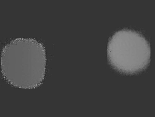
Fig. 4: The greyscale offset-compensation matrix, $A_{ij}$ for each half of the SLM. Black pixels (zero greyscale) represent zero imparted phase and white pixels (255 greyscale) represent a maximum imparted phase. On average, the compensation requires roughly 2.25 rad of phase about $\mathbf{S_{2}}$ and 0.86 rad of phase about $\mathbf{S_{1}}$.

With this compensation in place, the system should not modify the input polarization. Thus, the output polarization $\bar{\mathbf{S}}^{\prime}$ should be identical to any chosen input polarization. We test this with the nominal uniform input polarization state, $\mathbf{S}_{\mathrm{ideal}}=[0,1,0]$. This is our target state. To distinguish the performance of the polarization system from our ability to produce and measure polarizations, we also characterize the nominal input state by sending it directly to the polarimetry setup. We call the latter the experimental input state. In Table 1, we compare the target state to the experimental input, the output without compensation, and the output with compensation. When the phase compensation is used, the fidelity of $\bar{\mathbf{S}}^{\prime}$ with respect to the target input state improves by a percent difference of 85%, and the uniformity improves by a percent difference of 5%. Both measures indicate that the compensation significantly improves the system performance.

Table 1: Performance evaluation of phase-offset compensation.

State	Avg. Stokes Vector, $\bar{\mathbf{S}}_{\mathrm{exp}}$	Fidelity, $F$	Uniformity, $U$
input, target	$\mathbf{\mathbf{S}_{\mathrm{ideal}}}$ = [0,1,0]	1	1
experimental input	$\bar{\mathbf{S}}$ = [0.075, 0.986, 0.012]	0.993	0.988
w/o compensation	$\bar{\mathbf{S}}^{\prime}$ = [0.244, 0.056, -0.889]	0.528	0.924
with compensation	$\bar{\mathbf{S}}^{\prime}$ = [-0.114, 0.957, 0.071]	0.978	0.966

* The fidelity is $F=F(\bar{\mathbf{S}}{}_{\mathrm{exp}},\mathbf{S}{}_{\mathrm{ideal}})$.

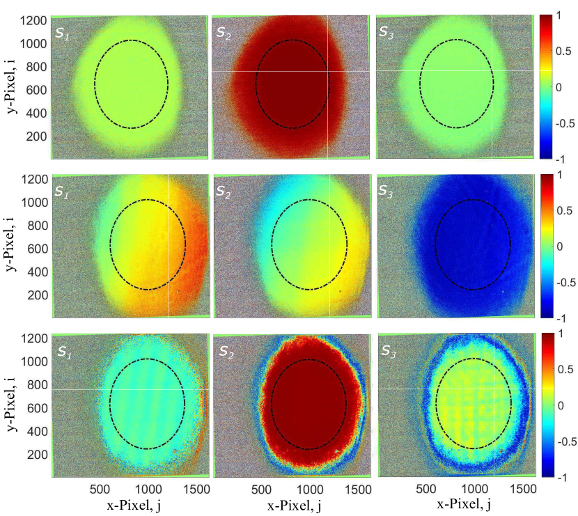
Fig. 5: Performance of the phase offset compensation. Each density plot shows the Stokes components across the wave front for $s_{1}$, $s_{2}$, and $s_{3}$ organized from left to right, and the black dotted line corresponds to the FWTM beam waist. The first row contains density plots for an experimentally measured input state $\mathbf{S}_{ij}$. Ideally, $\mathbf{S}_{ij}=\mathbf{S}_{\mathrm{ideal}}=[0,1,0]$. This data characterizes the performance of our polarimetry and input polarization state production. The other rows contain density plots for the measured output state for the input $\mathbf{S}_{ij}$ when there is no phase compensation (second row) and when there is phase compensation (third row). If the phase compensation was completely perfect, the first and third rows would be identical.

5 Experimental Results

5.1 Uniform to Non-Uniform Transformations

To demonstrate the capability of performing non-uniform polarization transformations, in this section we transform a uniformly $\ket{D}$-polarized beam to a different output polarization in each quadrant of the light field. We choose target states $\mathbf{S}^{\prime}_{\mathrm{ideal}}$ that constitute a set forming a symmetric, informationally complete positive-operator valued measure (SIC-POVM) [31]. These are known to be optimal for performing quantum polarization state tomography [31]. When the SIC-POVM states are plotted on the Poincaré sphere, the Stokes vector tips point to the vertices of a tetrahedron. Since they are equally distributed around the Poincaré sphere, our ability to produce them is a good indication that any arbitrary output polarization can be created.

Table 2: Performance of uniform to non-uniform transformations.

	Quadrant 1	Quadrant 2	Quadrant 3	Quadrant 4
$\mathbf{S}^{\prime}_{\mathrm{ideal}}$	$\frac{-1}{\sqrt{3}}[1,1,1]$	$\frac{1}{\sqrt{3}}[-1,1,1]$	$\frac{1}{\sqrt{3}}[1,1,-1]$	$\frac{1}{\sqrt{3}}[1,-1,1]$
$\bar{\mathbf{S}}^{\prime}_{\mathrm{exp}}$	$[-0.44,-0.70,-0.51]$	$[-0.50,0.58,0.51]$	$[0.53,0.41,-0.48]$	$[0.49,-0.43,0.61]$
$U$	0.93	0.88	0.88	0.95
$F$	0.96	0.94	0.93	0.97

*The uniformity is $U$. The fidelity is $F=F(\bar{\mathbf{S}}^{\prime}_{\mathrm{exp}},\mathbf{S}^{\prime}_{\mathrm{ideal}})$, where $\bar{\mathbf{S}}^{\prime}_{\mathrm{exp}}$ is the measured state and $\mathbf{S}^{\prime}_{\mathrm{ideal}}$ is the target state. Note that $\frac{1}{\sqrt{3}}=0.58.$

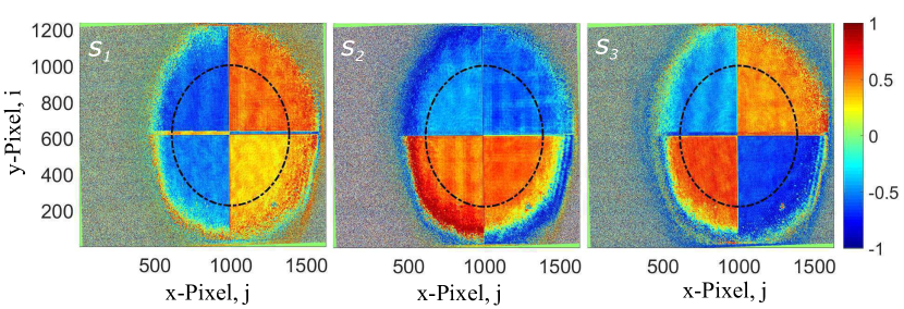
Fig. 6: The Stokes components for an ouput light field that contains polarization states equally distributed around the Poincaré sphere. Each quadrant is transformed to contain one such SIC-POVM state. For the purpose of Table 3, the quadrants are numbered starting from the bottom left and moving clockwise.

The results of this transformation are given in Table 2. The experimental average Stokes vector for each output quadrant $\bar{\mathbf{S}}^{\prime}_{\mathrm{exp}}$ are calculated over a circular sector (i.e., wedge) $A$ wholly within that quadrant. The fidelities of the four quadrants with respect to their target polarization states range from 0.93 to 0.97 and the uniformities range from 0.88 to 0.95. While all the states are produced reasonably well, the uniformity is significantly lower in some quadrants than others. Our investigations into this effect revealed that each pixel actually has a different axis of rotation in the Poincaré sphere, as seen in Fig. 7. In some cases, this difference is quite large and can change the intended transformation of one pixel by a phase corresponding to as much as ten greyscale increments. This error will also be more profound for some states than others. In particular, the axes differ in such a way that any state with a negative $s_{2}$ component will be constructed more accurately than states with a positive $s_{2}$ component.

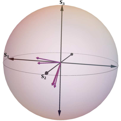
Fig. 7: The axes of rotation are plotted for five distinct SLM pixels in the FWTM beam waist. These particular axes exhibit the greatest deviations from the ideal axis of rotation, $\mathbf{S_{2}}$, and this deviation can be as large as 0.29 rad.

Another cause for imperfect results is the presence of a grid-like pattern in polarization that shows up in the density plots of the Stokes parameters (e.g., Fig. 5). This grid-like polarization effect is thought to be a diffraction effect from the pixels of the SLM. One can see in Fig. 4 that this pattern is noticeable at the greyscale level.

5.2 Painting with Polarization

While this non-uniform transformation successfully resulted in the desired state, only four distinct transformations were performed at once. This is a small number of transformations when one considers that each pixel of the SLM can transform light independently. To demonstrate this versatility we use the setup to implement polarization imaging. Here, full images can be encoded in polarization that are hidden to humans, a species whose vision is mostly polarization insensitive, but can be revealed through Stokes polarimetry and graphical representations of polarization.

Here, a cropped image of Van Gogh’s painting Starry Night was encoded in polarization. This painting is ideal for this because of its characteristic feature, the distinctly clear brush strokes that form swirls reminiscent of a vector field. Each region $(i,j)$ of the painting is converted to a target polarization state $\mathbf{S}^{\prime}_{ij}$. The darkness $D(i,j)$ of the region sets the polarization ellipticity through $s_{3,ij}=1-2(D(i,j)/D_{max})$, where $D_{max}$ is the maximum darkness in the painting. The angle $\psi(i,j)$ of the brush stroke in the region is converted to the dominant polarization direction through $s_{1,ij}=\sqrt{1-s_{3,ij}^{2}}\cos(2\psi(i,j))$ and $s_{2,ij}=\sqrt{1-s_{3,ij}^{2}}\sin(2\psi(i,j))$. With this target $\mathbf{S}^{\prime}_{ij}$ and a known input polarization $\mathbf{S}{}_{ij}$, the two-step scheme can be used to imprint a polarization image of Starry Night on a light field. We do so with a nominal uniformly diagonally polarized input field, $\mathbf{S}=[0,1,0]$. A species that could see linear polarization (e.g., octopus or mantas shrimp) might be able to perceive this image directly. Conceivably, they would see something similar to the left image in Fig. 8, where we have converted the polarizations $\mathbf{S}^{\prime}_{ij}$ back to line segments at angles $\psi(i,j)$. The darkness $D(i,j)$ sets the thickness of the line segment. We, however, must use our Stokes polarimetry setup to perceive the image. We similarly convert the experimentally measured Stokes vectors to the right image in Fig. 8. It is, unmistakably, Starry Night, therein demonstrating our ability to effectively paint with polarization.

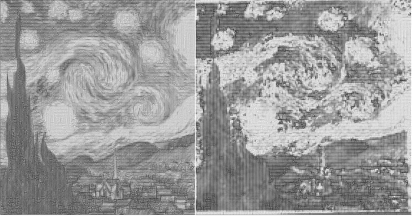
Fig. 8: Van Gogh’s painting Starry Night, painted in polarization. On the left is the simulated target image, on the right is the experimental result. In each region, the line segment angle corresponds to the dominant polarization direction. The thickness of the line segment is set by the ellipticity of the polarization in that region of the light field.

5.3 Non-Uniform to Uniform Transformations

Performing non-uniform-to-uniform transformations may also offer applications in beam healing, where polarization aberrations and undesired non-uniformities can be corrected for by bringing a light field back to a uniform polarization state. To demonstrate that the setup is capable of these transformations, a liquid crystal cell with a spatially varying optic axis orientation was added between the input polarization state preparation stage and the two-step scheme setup. This transforms a uniform, circularly polarized state to a highly non-uniform polarization input state. With only the phase-offset compensation in place, we measured this non-uniform polarization profile. We took this pre-corrected state as our input $\mathbf{S}{}_{ij}$. We then used the setup to transform to the uniformly polarized target state, $\mathbf{S}^{\prime}_{\mathrm{ideal}}=[0,0,1]$. The experimentally measured pre-corrected state $\mathbf{S}{}_{ij}$ and corrected state $\mathbf{S}^{\prime}_{ij}$ are respectively shown in the top and bottom of Fig. 9. To the eye, the uniformity of the light field is considerably improved. As summarized in Table 3, this impression is confirmed by the nearly 40% increase in uniformity of the light field. This demonstrates that the two-step scheme can be used to heal polarization aberrations in beams.

Table 3: Homogenizing a highly non-uniformly polarized light field towards a target of $\mathbf{S}^{\prime}_{\mathrm{ideal}}=[0,0,1]$.

Polarization field	Avg. Stokes vector, $\bar{\mathbf{S}}{}_{\mathrm{exp}}$	Fidelity, $F(\bar{\mathbf{S}}_{\mathrm{exp}},\mathbf{S}^{\prime}_{\mathrm{ideal}})$	Uniformity, $U$
Pre-corrected state, $\mathbf{S}{}_{ij}$	$\bar{\mathbf{S}}$	0.799	0.632
Corrected state, $\mathbf{S}^{\prime}{}_{ij}$	$\bar{\mathbf{S}}^{\prime}$	0.933	0.869
% Difference		17 %	38 %

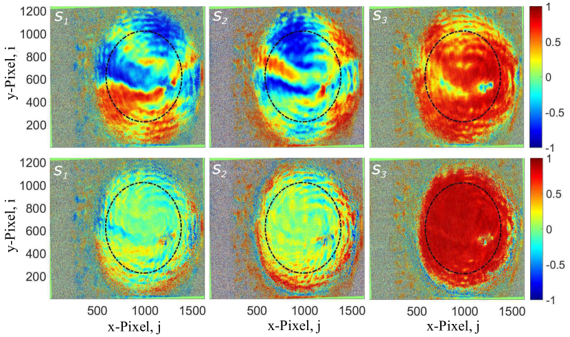
Fig. 9: Correcting polarization aberrations. We transform a light field with a highly non-uniform polarization $\mathbf{S}_{ij}$ (top row) to a more uniform polarization $\mathbf{S}^{\prime}_{ij}$ (bottom row).

6 Conclusion

We have shown that two-step polarization transformations can be used to produce arbitrary, spatially varying polarization states from a known polarization state. In particular, polarizations in each quadrant of a wave front were produced as desired with fidelities upwards of 0.93. It was also shown that these transformations can be used to paint with polarization, where Van Gogh’s painting Starry Night was embedded in the polarization of a light field through the use of elliptical polarization states. Finally, it was shown that these transformations can be used to ‘heal’ the polarization of a light field, where a light field with an initial uniformity of 0.632 was transformed to have a uniformity of 0.869.

Future directions of this work include using the system to perform transformations that bring a non-uniform state to another non-uniform state. Such transformations would be useful in spatially multiplexed polarization-based quantum cryptography. Another noteworthy application is the non-diffractive patterning of passive liquid crystal devices. Standard techniques used to pattern liquid crystal devices use photoalignment methods involving a digital micro-mirror device (DMD) for micro-lithography [32]. In them, arbitrarily complex liquid crystal patterns are created by sequentially exposing various regions of a dye or polymer to various polarizations. The two-step scheme would require only a single exposure, thereby increasing production throughput. These patterned liquid crystal devices (e.g., q-plates) are static. They are each designed to generate select subsets of vector beams. In contrast, the two-step scheme can create any arbitrary spatial polarization, which itself can be changed at a rate of 60 Hz. If transmissive SLMs are improved, one may reduce the complexity of the setup by using transmissive devices in place of reflective ones in order to avoid stray reflections and their associated spurious optical interference. As well, transmissive SLMs would make experiments based on three successive phase modulations more feasible. These could implement even more general transformations than those presented here, transformations with an arbitrary Poincaré sphere axis and angle of rotation at each pixel [25].

Funding

This research was undertaken, in part, thanks to funding from the following organizations: Canada Research Chairs, NSERC Discovery, Canada Foundation for Innovation, Canada First Research Excellence Fund, and Canada Excellence Research Chairs program.

Appendix

A1 Alignment and Mapping of the SLM to the CCD

For the two-step scheme to function we must program particular SLM pixels to modify particular regions of the light field. We now describe an alignment procedure and mapping between the pixels illuminated by the light field on each of the two separate incidences of the SLM, $(i_{1}^{SLM},j_{1}^{SLM})$ and $(i_{2}^{SLM},j_{2}^{SLM})$, and the pixels of the CCD camera, $(i^{CCD},j^{CCD})$, which are at position $(x_{j},y_{i})$ of the wave front. The alignment and mapping is accomplished by displaying a fiducial greyscale pattern on each half of the SLM. In the left of Fig. 10, we show this pattern in the case when it is present only on the left half of the SLM. After passing through the SLM part of the setup, the light travels through the Stokes polarimetry apparatus to form a clear image of the pattern on the CCD, as shown on the right in Fig. 10. Our mapping function, this vector formula, compensates for four issues: scaling, offset, reflection, and rotation:

$$\begin{bmatrix}i_{k}^{SLM}-i_{k,0}^{SLM}\\ j_{k}^{SLM}-j_{k,0}^{SLM}\end{bmatrix}=\begin{bmatrix}\cos\theta_{k}&-\sin\theta_{k}\\ \sin\theta_{k}&\cos\theta_{k}\end{bmatrix}\begin{bmatrix}\lfloor m_{k,y}\left(i^{CCD}-i_{0}^{CCD}\right)\rfloor\\ \lfloor m_{k,x}\left(j^{CCD}-j_{0}^{CCD}\right)\rfloor\end{bmatrix}.$$ (4)

In the following sections, we explain this mapping, define the parameters in it, and describe how they were determined.

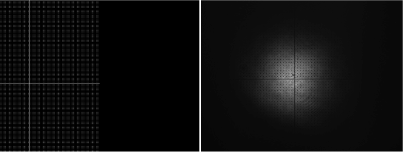
Fig. 10: The fiducial greyscale pattern on the left half of the SLM (left) and the resulting image on the CCD (right).

A1.1 Image Offset

The pattern on each half of the SLM has an offset in reference to the CCD array. The image of the bright central cross-hair in Fig. 10 from the left and right halves of the SLM were manually aligned to the center of the light field by shifting the corresponding greyscale patterns. The exact position of the cross-hair on the CCD is used to set an origin for the CCD $(i_{0}^{CCD},j_{0}^{CCD})$, as well as the two SLM offsets $(i_{k,0}^{SLM},j_{k,0}^{SLM}$), where $k=1,2$ corresponding to the left and right half of the SLM. This fixes all the pixel offsets in Eq. (4).

A1.2 Image Scaling

While the $4f$ imaging nominally has a magnification of one, it might deviate from this experimentally. As well, the pixel sizes of the CCD and SLM are different. We account for these issues with two components in our mapping, scaling and resampling. The scaling is accounted for by the $m_{k,y}$ and $m_{k,x}$ magnification factors in Eq. (4), for the first and second SLM halves, $k=1,2$. We determine these factors using the grid of dots in the fiducial pattern. To accurately determine the scaling we take a Fourier transform of the CCD image to determine the spatial frequency of the pattern. With this, we determine that $m_{y}=0.209$ and $m_{x}=0.208$. Identical results were obtained for both halves of the SLM, so we have dropped the $k$ subscript for now. According to the pixel size specifications of the CCD and SLM, and if we had an optical magnification of one, we would expect $m_{x}=m_{y}=0.22$. This is $5.5\%$ larger than the experimental values.

Since the magnification factors are less than one, there are $1/m_{x}m_{y}$ CCD pixels for each SLM pixel. This many-to-one mapping, i.e., resampling, is accomplished using a floor function, denoted by the $\lfloor\rfloor$ symbols in Eq. (4). The floor function rounds to the nearest lower integer. In doing so it fixes only one CCD pixel to correspond to each SLM pixel. An alternative would be to average over a region of $1/m_{x}m_{y}$ CCD pixels to derive one effective CCD pixel for each SLM pixel. Standard imaging specific resampling functions (e.g., bicubic) could also be used, though these are less transparent in their functioning. All three methods were attempted and flooring was chosen as the most robust in its functioning.

A1.3 Image Reflections

There are multiple sources of image flips (e.g., invert horizontally, $x\rightarrow-x$) in the system. These flips can occur between incidences on the SLM and between the SLM and CCD. Every reflection from a mirror, beamsplitter or the SLM will invert $x$. Each $4f$ lens system inverts both $x$ and $y$. Lastly, the orientation (i.e., the default direction of increasing pixel number) of the CCD sensor can be different from that of the SLM. Mathematically, this translates to negation of either or both magnification factors, $m_{k,y}$ and $m_{k,x}$ for Eq. (4) for the first and second SLM halves, $k=1,2$. These negations can be determined by placing non-symmetric images (e.g., the letter F) on each of the two SLM halves and simply observing on the CCD in which directions they have each been flipped. In our system, only the second half of the SLM must be flipped. Consequently, the magnification factor $m_{2,x}=-0.208$ has been negated.

A1.4 Image Rotation

The image can rotate if the light propagation axis is not parallel with the optical table. This deviation from parallel occurs in some places in our setup, as is evident by the offset between the left and right greyscale patterns in Fig. 4. We incorporated this rotation in Eq. (4) with a standard rotation matrix that rotates the $x-y$ plane by an angle of $\theta_{k}$. This rotation can be determined directly by the orientation of the cross-hair or through a Fourier transform of the grid of dots in the fiducial pattern. From this, we find that there is no rotation between the second half of the SLM and the CCD. However, the fiducial on the first half on the SLM appears rotated relative the CCD sensor edges by $0.0321$ radians. We set $\theta_{1}=0$ and $\theta_{2}=0.0321$ radians so that light incident on a pixel on the second half of the SLM is reflected from the corresponding pixel on the first have of the SLM. i.e., $i_{1}^{SLM}=i_{2}^{SLM}$ and $j_{1}^{SLM}=j_{2}^{SLM}$. The result is that fiducials that are aligned with the pixel columns on the first and second half of the SLM will appear on CCD exactly aligned (i.e., superposed). However, they will be rotated with respect to CCD sensor axes. We rotate the final image is back by $-\theta_{2}$ during post-processing to ensure the polarization pattern (and fiducial) appears upright as intended. In any of the experimental density plots of the Stokes components, one can see signs of this rotation at the plot edges.

A1.5 Nonlinear Image Distortion

We also used the fiducial grid to look for evidence of a nonlinear component to our mapping, such as pincushion or barrel distortion. Such distortions are not included in our linear mapping, Eq. (4). We measured the grid spacing across the extent of the CCD image. To within an uncertainty equal to the width of the image of a grid dot, we observed no variation in the grid spacing, confirming the absence of nonlinear image distortion.

A2 Calculating Required Retardances

For a desired transformation from $\mathbf{S}=[s_{1},s_{2},s_{3}]$ to $\mathbf{S}^{\prime}=[s^{\prime}_{1},s^{\prime}_{2},s^{\prime}_{3}]$, the retardances $\zeta_{1}$ and $\zeta_{2}$ must be calculated for each desired transformation. They are given by Sit et al. [25] as,

$$\zeta_{1}=\mathrm{atan2}\left([0,s_{2},s_{3}]\cdotp[0,s^{\prime\prime}{}_{2},s^{\prime\prime}{}_{3}],\textrm{sgn}(s_{2}s^{\prime\prime}{}_{3}-s_{3}s^{\prime\prime}{}_{2})\left|[0,s_{2},s_{3}]\times[0,s^{\prime\prime}{}_{2},s^{\prime\prime}{}_{3}]\right|\right)\textrm{ mod }2\pi$$ (5)

$$\zeta_{2}=\mathrm{atan2}\left([s^{\prime\prime}_{1},0,s^{\prime\prime}{}_{3}]\cdotp[s^{\prime}_{1},0,s^{\prime}_{3}],\textrm{sgn}(s^{\prime}_{1}s^{\prime\prime}{}_{3}-s^{\prime}_{3}s^{\prime\prime}{}_{1})\left|[s^{\prime\prime}_{1},0,s^{\prime\prime}{}_{3}]\times[s^{\prime}_{1},0,s^{\prime}_{3}]\right|\right)\textrm{ mod }2\pi$$ (6)

$$\mathbf{S}^{\prime\prime}=\left[s_{1},s^{\prime}_{2},\textrm{sgn}\left(s^{\prime}_{3}\right)\left(\left(s_{3}\right)^{2}+\left(s_{2}\right)^{2}-\left(s^{\prime}_{2}\right)^{2}\right)^{(1/2)}\right]=[s^{\prime\prime}{}_{1},s^{\prime\prime}{}_{2},s^{\prime\prime}{}_{3}]$$ (7)

Where $\mathbf{S}^{\prime\prime}=\hat{R}(\mathbf{S_{1}},\zeta_{1})\mathbf{S}$ is an intermediate polarization state resulting from the first rotation and serves as the starting point for the second rotation. The four quadrant inverse tangent function, $-\pi\leq\mathrm{atan2(x,y)\leq\pi}$, gives the angle from the positive $x$ axis to the point $(x,y)$. The $\mathrm{sgn}$ function is the signum function with the convention $\mathrm{sgn}(0)=1$. The modulo function $\mathrm{mod}2\pi\geq 0$ by convention, and $\times$ and $\cdot$ are the standard cross and dot products, respectively. Geometrically, $\zeta_{1}$ is the positive angle between the projections of the $\mathbf{S}$ and $\mathbf{S}^{\prime\prime}$ vectors onto the $\mathbf{S_{2}}-\mathbf{S_{3}}$ plane. Similarly, $\zeta_{2}$ is the positive angle between the projections of the $\mathbf{S}^{\prime\prime}$ and $\bar{\mathbf{S}}^{\prime}$vectors onto the $\mathbf{S_{1}}-\mathbf{S_{3}}$ plane.