Optimal Actuator Design for Semi-linear Systems

Abstract

Actuator location and design are important choices in controller design for distributed parameter systems. Semi-linear partial differential equations model a wide spectrum of physical systems with distributed parameters. It is shown that under certain conditions on the nonlinearity and the cost function, an optimal control input together with an optimal actuator choice exists. First-order necessary optimality conditions are derived. The results are applied to optimal actuator and controller design in a nonlinear railway track model as well as semi-linear wave models.

49J27, 49K27, 49J20, 49J50, 35L71

1 Introduction

Actuator location and design are important design variables in controller synthesis for distributed parameter systems. Finding the best actuator location to control a distributed parameter system can significantly reduce the cost of the control and improve its effectiveness; see for example, [19, 39, 40]. The optimal actuator location problem has been discussed by many researchers in various contexts; see [22, 53] for a review of applications and [44] for optimal location of actuators to maximize controllability in the wave equation. In [38], it was proved that an optimal actuator location exists for linear-quadratic control. Conditions under which using approximations in optimization yield the optimal location are also established. Similar results have been obtained for $H_{2}$ and $H_{\infty}$ controller design objectives with linear models [27, 41]. Results for optimal design of linear PDE’s have been obtained [26, 42]. There are also results on the related problem of optimal sensor location for linear PDE’s; see [45] for locations of maximum observability in the wave equation and [55, 58] for concurrent sensor choice/estimator design to minimize the error variance.

Nonlinearities can have a significant effect on dynamics, and such systems cannot be accurately modelled by linear differential equations. Optimal control of systems modelled by nonlinear partial differential equations (PDE’s) has been studied for a number of applications, including wastewater treatment systems [34], steel cooling plants [52], oil extraction through a reservoir [32], solidification models in metallic alloys [8], thermistors [25], Schlögl model [9, 11], FitzHugh–Nagumo system [11], static elastoplasticity [15], type-II superconductivity [56], Fokker-Planck equation [21], Schrödinger equation with bilinear control [13], Cahn-Hilliard-Navier-Stokes system [23], wine fermentation process [35], time-dependent Kohn-Sham model [50], elastic crane-trolley-load system [29]. A review of PDE-constrained optimization theory can be found in the books [24, 31, 51]. State-constrained optimal control of PDEs has also been studied. In [7], the authors investigated the structure of Lagrange multipliers for state constrained optimal control problem of linear elliptic PDEs. Research on optimal control of PDEs, such as [10, 46], has focused on parabolic models of partial differential equations with certain structures. Optimal control of differential equations in abstract spaces has rarely been discussed [36]. This paper extends previous results to abstract differential equations without an assumption of stability.

Optimal actuator location has been addressed for some applications modeled by nonlinear distributed parameter systems using a finite dimensional approximation of the original partial differential equation model. In [3], authors investigated the optimal actuator and sensor location problem for a transport-reaction process using a finite-dimensional model. Similarly, in [33], the optimal actuator and sensor location of Kuramoto-Sivashinsky equation was studied using a finite-dimensional approximation. Other research concerned with optimal actuator location in problems with nonlinear distributed parameter dynamics can be found in [4, 37, 47]. To our knowledge, there are no theoretical results on optimal actuator location of nonlinear PDE’s.

Theory for concurrent optimal control and actuator design of a class of controlled semi-linear PDE’s is described in this paper. The research described extends previous work on optimal control of PDE’s in that the linear part of the partial differential equation is not constrained to be the generator of an analytic semigroup. The input operator of the system is parametrized by the possible actuator designs. A general class of PDE’s with weakly continuous nonlinear part is considered. Optimality equations explicitly characterizing the optimal control and actuator are obtained.

Location of actuators on flexible structures has been one of the motivators for research into optimal actuator location [22]. Various models have been studied. Classical results in the literature concern control of linear and nonlinear Euler Bernoulli and Timoshenko beam models [28, 30, e.g.]. In recent years, non-classical models of flexible beams such as micro-beam models have also attracted attention [16, e.g.]. In nonlinear flexible structures, the nonlinearity typically is on deformations, not on the rate of deformations. The space in which deformations evolve is compactly embedded in that of rate of deformations. As a result, the nonlinear terms are weakly continuous in the underlying state space. One application of the results in this paper is to the development of an optimal control strategy for the vibration suppression of railway tracks [2, 14, 17]. The theory is also illustrated by application to concurrent optimal control and actuator design for semi-linear waves in two space dimensions.

The paper is organized as follows. After a short paragraph on notation, the problem definition as well as the main results are stated in section 2. Section 3 discusses the existence of a solution to the semi-linear partial differential equation. The existence of an optimizer is established in section 4. First-order necessary condition for the optimizer are provided in section 5. In section 6 and 7, the results of the previous sections are applied to the railway track model and semi-linear wave models, respectively.

Notation

Throughout this paper, the letters $c$, $t$, and $\xi$ denote a generic positive constant, temporal variable, and spatial variable, respectively. The blackboard letters as in ${\mathbb{X}}$ denote Banach spaces, the calligraphic letters as in $\mathcal{A}$ denote operators on a Banach space. If an operator is nonlinear its argument is shown in parenthesis as in ${\mathcal{F}}(\cdot)$. The bold letters as in ${\bm{x}}$ refer to states evolving in a Banach space; the rest of letters represent physical or generic constants. The adjoint of an operator is denoted by $\mathcal{A}^{*}$. The superscript ${\cdot}^{o}$ shows that a state or an input is optimal, and the tilde overscript $\tilde{\cdot}$ is reserved for the state of a linearized system unless otherwise stated. Norms and inner products on the underlying state space are typed without any subscript, but on any other spaces, they are shown with a suitable subscript to avoid confusion. The norm on $L^{p}(0,\tau;{\mathbb{U}})$ is denoted by $\left\|\cdot\right\|_{p}$. Strong convergences on a Banach space are shown by $\to$, whereas a weak convergence is shown by $\rightharpoonup$. If the Banach space ${\mathbb{X}}_{1}$ is continuously embedded in ${\mathbb{X}}_{2}$, we write ${\mathbb{X}}_{1}\hookrightarrow{\mathbb{X}}_{2}$. The Banach space $C([0,\tau];{\mathbb{X}})$ will often be indicated by $C(0,\tau;{\mathbb{X}})$ for simplicity of notation.

2 Main Results

Consider a semi-linear system with state ${\bm{x}}(t)$ on a separable reflexive Banach space ${\mathbb{X}}$:

(1) $$\dot{{\bm{x}}}(t)=\mathcal{A}{\bm{x}}(t)+{\mathcal{F}}({\bm{x}}(t))+\mathcal{B}({\bm{r}}){\bm{u}}(t),\quad{\bm{x}}(0)={\bm{x}}_{0}\in{\mathbb{X}},$$

The function ${\bm{u}}(t)$ is the input to the system, and takes values in a reflexive Banach space ${\mathbb{U}}$. The control operator $\mathcal{B}({\bm{r}})$ depends on a parameter ${\bm{r}}$ that takes values in a set $K_{ad}$ in a topological space $\mathbb{K}$. The parameter ${\bm{r}}$ typically has interpretation as possible actuator designs. The operators $\mathcal{A}$, ${\mathcal{F}}(\cdot)$, and $\mathcal{B}(\cdot)$ satisfy the following assumptions.

Assumption A.

1. The state operator $\mathcal{A}$ with domain $D(\mathcal{A})$ generates a strongly continuous semigroup $\mathcal{T}(t)$ on ${\mathbb{X}}$.

2. Let ${\mathcal{F}}(0)=0$; the nonlinear operator ${\mathcal{F}}(\cdot)$ is locally Lipschitz continuous on ${\mathbb{X}}$; that is, for every positive number $\delta$, there exists $L_{{\mathcal{F}}\delta}>0$ such that

   $$\left\|{\mathcal{F}}({\bm{x}}_{2})-{\mathcal{F}}({\bm{x}}_{1})\right\|\leq L_{{\mathcal{F}}\delta}\left\|{\bm{x}}_{2}-{\bm{x}}_{1}\right\|,$$

   for all $\left\|{\bm{x}}_{2}\right\|\leq\delta$ and $\left\|{\bm{x}}_{1}\right\|\leq\delta$.

3. For each ${\bm{r}}\in K_{ad}$, the input operator $\mathcal{B}({\bm{r}})$ is a linear bounded operator that maps the input space ${\mathbb{U}}$ into the state space ${\mathbb{X}}$. This family of operators is uniformly bounded over $K_{ad}$, i.e., there exist a positive number $M_{\mathcal{B}}$ such that $\left\|\mathcal{B}({\bm{r}})\right\|_{\mathcal{L}({\mathbb{U}},{\mathbb{X}})}\leq M_{\mathcal{B}}$ for all ${\bm{r}}\in K_{ad}$.

In some cases, due to lack of regularity of the input ${\bm{u}}$, a classical solution to (1) is not assured.

Definition 2.1.

If ${\bm{x}}\in C(0,\tau;{\mathbb{X}})$ satisfies

(2) $${\bm{x}}(t)=\mathcal{T}(t){\bm{x}}_{0}+\int_{0}^{t}\mathcal{T}(t-s){\mathcal{F}}({\bm{x}}(s))ds+\int_{0}^{t}\mathcal{T}(t-s)\mathcal{B}({\bm{r}}){\bm{u}}(s)ds,$$

for every ${\bm{x}}_{0}\in{\mathbb{X}}$, it is said to be a mild solution to (1).

In Section 3, the existence of a unique mild solution to the initial value problem (IVP) (1) is proven for ${\bm{u}}(t)$ in the set

$$U_{ad}=\{{\bm{u}}\in L^{p}(0,\tau;{\mathbb{U}}):\,\left\|{\bm{u}}\right\|_{p}\leq R\},$$

where $1<p<\infty$.

Theorem 3.1: Under assumption A, for each ${\bm{x}}_{0}\in{\mathbb{X}}$ and positive number $R$, there exists $\tau>0$ such that (1) admits a unique local mild solution ${\bm{x}}\in C(0,\tau;{\mathbb{X}})$ for all ${\bm{u}}\in U_{ad}$, and all ${\bm{r}}\in K_{ad}$.

For functionals $\phi({\bm{x}})$ on ${\mathbb{X}}$ and $\psi({\bm{u}})$ on ${\mathbb{U}}$, consider the cost function

$$J({\bm{u}},{\bm{r}};{\bm{x}}_{0})=\int_{0}^{\tau}\phi({\bm{x}}(t))+\psi({\bm{u}}(t))\,dt.$$

The optimization problem is to minimize $J({\bm{u}},{\bm{r}};{\bm{x}}_{0})$ over all admissible control inputs ${\bm{u}}\in U_{ad}$, and also over all admissible actuator designs ${\bm{r}}\in K_{ad}$, subject to (1) with a fixed initial condition ${\bm{x}}_{0}\in{\mathbb{X}}$. That is,

(P) $$\left\{\begin{array}[]{ll}\min&J({\bm{u}},{\bm{r}};{\bm{x}}_{0})\\ \text{s.t.}&\dot{{\bm{x}}}(t)=\mathcal{A}{\bm{x}}(t)+{\mathcal{F}}({\bm{x}}(t))+\mathcal{B}({\bm{r}}){\bm{u}}(t),\quad\forall t\in(0,\tau],\\ &{\bm{x}}(0)={\bm{x}}_{0},\\ &{\bm{u}}\in U_{ad},\\ &{\bm{r}}\in K_{ad}.\end{array}\right.$$

To guarantee the existence of a unique optimizer, further assumptions are needed on the operators ${\mathcal{F}}(\cdot)$, $\mathcal{B}(\cdot)$, the set $K_{ad}$, and the cost function $J({\bm{u}},{\bm{r}};{\bm{x}}_{0})$.

Assumption B.

1. Let ${\bm{x}}_{n}(t)$ be a bounded sequence in $C(0,\tau;{\mathbb{X}})$ such that ${\bm{x}}_{n}\rightharpoonup{\bm{x}}$ in $L^{p}(0,\tau;{\mathbb{X}})$. Then, ${\mathcal{F}}({\bm{x}}_{n})\rightharpoonup{\mathcal{F}}({\bm{x}})$ in $L^{p}(0,\tau;{\mathbb{X}})$.

2. Let $K_{ad}$ be a compact convex set in the actuator design space $\mathbb{K}$. The family of input operators $\mathcal{B}(\cdot):K_{ad}\to\mathcal{L}({\mathbb{U}},{\mathbb{X}})$ are continuous with respect to ${\bm{r}}$ in the operator norm topology:

   $$\lim_{{\bm{r}}_{2}\to{\bm{r}}_{1}}\left\|\mathcal{B}({\bm{r}}_{2})-\mathcal{B}({\bm{r}}_{1})\right\|_{\mathcal{L}({\mathbb{U}},{\mathbb{X}})}=0.$$

3. The functionals $\phi(\cdot)$ and $\psi(\cdot)$ are weakly lower semi-continuous non-negative functionals on ${\mathbb{X}}$ and ${\mathbb{U}}$, respectively.

It is shown in Section 4 that under these assumptions, an optimal control and actuator design exist.

Theorem 4.1: For initial condition ${\bm{x}}_{0}\in{\mathbb{X}}$, let $\tau$ be such that the mild solution exists for all ${\bm{u}}\in U_{ad}$, and all ${\bm{r}}\in K_{ad}$. Under assumptions A and B, there exists a control input ${\bm{u}}^{o}\in U_{ad}$ together with an actuator design ${\bm{r}}^{o}\in K_{ad}$, that solves the optimization problem P.

To characterize an optimizer to the optimization problem, further assumptions on differentiability of the nonlinear operators $\mathcal{F}(\cdot)$ and ${\mathcal{B}}(\cdot)$, and the cost function are needed.

Assumption C.

1. The nonlinear operator ${\mathcal{F}}(\cdot)$ is Gâteaux differentiable on ${\mathbb{X}}$ ([24, Def. 1.29]). Indicate the Gâteaux derivative of ${\mathcal{F}}(\cdot)$ at ${\bm{x}}$ in the direction ${\bm{p}}$ by ${\mathcal{F}}^{\prime}_{{\bm{x}}}{\bm{p}}$. Furthermore, the mapping ${\bm{x}}\mapsto{\mathcal{F}}^{\prime}_{{\bm{x}}}$ is bounded; that is, bounded sets in ${\mathbb{X}}$ are mapped to bounded sets in $\mathcal{L}({\mathbb{X}})$.

2. The control operator $\mathcal{B}({\bm{r}})$ is Gâteaux differentiable with respect to ${\bm{r}}$ from $K_{ad}$ to $\mathcal{L}({\mathbb{U}},{\mathbb{X}})$. Indicate the Gâteaux derivative of $\mathcal{B}({\bm{r}})$ at ${\bm{r}}^{o}$ in the direction ${\bm{r}}$ by $\mathcal{B}^{\prime}_{{\bm{r}}^{o}}{\bm{r}}$. Furthermore, the mapping ${\bm{r}}^{o}\mapsto{\mathcal{B}}^{\prime}_{{\bm{r}}^{o}}$ is bounded; that is, bounded sets in ${\mathbb{K}}$ are mapped to bounded sets in $\mathcal{L}({\mathbb{K}},\mathcal{L}({\mathbb{U}},{\mathbb{X}}))$.

3. The spaces ${\mathbb{X}}$, ${\mathbb{U}}$, and ${\mathbb{K}}$ are Hilbert spaces, and p=2. Also, in the cost function, set

   (3) $$\phi({\bm{x}})=\left\langle\mathcal{Q}{\bm{x}},{\bm{x}}\right\rangle,\quad\psi({\bm{u}})=\left\langle\mathcal{R}{\bm{u}},{\bm{u}}\right\rangle_{{\mathbb{U}}},$$

   where the linear operator $\mathcal{Q}$ is a positive semi-definite, self-adjoint bounded operator on ${\mathbb{X}}$, and the linear operator $\mathcal{R}$ is a positive definite, self-adjoint bounded operator on ${\mathbb{U}}$.

Since ${\mathbb{X}}$, ${\mathbb{U}}$, and ${\mathbb{K}}$ are assumed to be Hilbert spaces in assumption C3, the dual of each of these spaces can be identified with the space itself. The operator $(\mathcal{B}^{\prime}_{{\bm{r}}^{o}}{\bm{u}})^{*}:{\mathbb{X}}\to\mathbb{K}$ is defined as

$$\left\langle(\mathcal{B}^{\prime}_{{\bm{r}}^{o}}{\bm{u}})^{*}{\bm{p}},{\bm{r}}\right\rangle_{\mathbb{K}}=\left\langle{\bm{p}},(\mathcal{B}^{\prime}_{{\bm{r}}^{o}}{\bm{r}}){\bm{u}}\right\rangle,\quad\forall({\bm{u}},{\bm{p}},{\bm{r}})\in{\mathbb{U}}\times{\mathbb{X}}\times\mathbb{K}.$$

The following theorem is proved in Section 5. In this theorem ${\bm{x}}=\mathcal{S}({\bm{u}};{\bm{r}},{\bm{x}}_{0})$ denotes the control-to-state map (see Definition 5.1).

Theorem 5.10: Suppose assumptions A1 and C hold, For any initial condition ${\bm{x}}_{0}\in{\mathbb{X}}$, let the pair $({\bm{u}}^{o},{\bm{r}}^{o}){\in U_{ad}\times K_{ad}}$ be a local minimizer of the optimization problem P with the optimal trajectory ${\bm{x}}^{o}=\mathcal{S}({\bm{u}}^{o};{\bm{r}}^{o},{\bm{x}}_{0})$ and let ${\bm{p}}^{o}(t)$, the adjoint state, indicate the mild solution of the final value problem

$$\dot{{\bm{p}}}^{o}(t)=-(\mathcal{A}^{*}+{\mathcal{F}}^{\prime*}_{{\bm{x}}^{o}(t)}){\bm{p}}^{o}(t)-\mathcal{Q}{\bm{x}}^{o}(t),\quad{\bm{p}}^{o}(\tau)=0.$$

If $({\bm{u}}^{o},{\bm{r}}^{o})$ is in the interior of $U_{ad}\times K_{ad}$ then $({\bm{u}}^{o},{\bm{r}}^{o})$ satisfies

$${\bm{u}}^{o}(t)=-\mathcal{R}^{-1}\mathcal{B}^{*}({\bm{r}}^{o}){\bm{p}}^{o}(t),$$

$$\int_{0}^{\tau}(\mathcal{B}^{\prime}_{{\bm{r}}^{o}}{\bm{u}}^{o}(t))^{*}{\bm{p}}^{o}(t)\,dt.$$

3 Existence of a Solution to the IVP

In the existing literature, the existence of a unique local solution to (1) is guaranteed for continuously differentiable control inputs (see e.g. [43, Thm. 6.1.5]). Requiring that ${\bm{u}}\in C^{1}(0,\tau;{\mathbb{U}})$ is too restrictive for establishing existence of an optimal control. The following theorem guarantees the existence of a unique local mild solution under a weaker assumption on the input.

Theorem 3.1.

Under assumption A, for each ${\bm{x}}_{0}\in{\mathbb{X}}$ and positive number $R$, there exists $\tau>0$ such that (1) admits a unique local mild solution ${\bm{x}}\in C(0,\tau;{\mathbb{X}})$ for all ${\bm{u}}\in U_{ad}$, and all ${\bm{r}}\in K_{ad}$.

Proof 3.2.

The idea of the proof is similar to [43, Thm. 6.1.4], with a slight modification that here ${\bm{u}}(t)$ is in $L^{p}(0,\tau;{\mathbb{U}})$. For any ${\bm{x}}_{0}\in{\mathbb{X}}$ choose constants $\delta_{0}>0$ and $\tau>0$ such that for all $t\in[0,\tau]$

$$\left\|\mathcal{T}(t){\bm{x}}_{0}-{\bm{x}}_{0}\right\|\leq\delta_{0}.$$

Let $\mathbb{S}$ be the closed bounded subset of $C(0,\tau;{\mathbb{X}})$ defined as

(5) $$\mathbb{S}=\left\{{\bm{x}}\in C(0,\tau;{\mathbb{X}})|\;{\bm{x}}(0)={\bm{x}}_{0},\,\left\|{\bm{x}}(t)-{\bm{x}}_{0}\right\|\leq 2\delta_{0},\;\forall t\in[0,\tau]\right\}.$$

Define the operator $\mathcal{G}$ on $\mathbb{S}$ to be

(6) $$\mathcal{G}({\bm{x}})(t)=\mathcal{T}(t){\bm{x}}_{0}+\int_{0}^{t}\mathcal{T}(t-s){\mathcal{F}}({\bm{x}}(s))\,ds+\int_{0}^{t}\mathcal{T}(t-s)\mathcal{B}({\bm{r}}){\bm{u}}(s)\,ds.$$

It will be shown that for sufficiently small $\tau$, $\mathcal{G}$ maps $\mathbb{S}$ into $\mathbb{S}$ and is a contraction on $\mathbb{S}.$

Use the triangle inequality and write

(7) $$\left\|\mathcal{G}({\bm{x}})(t)-{\bm{x}}_{0}\right\|\leq \left\|\mathcal{T}(t){\bm{x}}_{0}-{\bm{x}}_{0}\right\|+\left\|\int_{0}^{t}\mathcal{T}(t-s){\mathcal{F}}({\bm{x}}(s))\,ds\right\|$$

$$+\left\|\int_{0}^{t}\mathcal{T}(t-s)\mathcal{B}({\bm{r}}){\bm{u}}(s)\,ds\right\|.$$

There exist a number $M_{{\mathcal{T}}}>0$ that $\left\|\mathcal{T}(t)\right\|\leq M_{{\mathcal{T}}}$ for all $t\in[0,\tau]$. Also, recall from assumption A2 that there is $L_{{\mathcal{F}}\delta}>0$ so that $\|{\mathcal{F}}({\bm{x}}(s))\|\leq L_{{\mathcal{F}}\delta}\|{\bm{x}}(s)\|$ on a ball of radius $\delta=\left\|{\bm{x}}_{0}\right\|+2\delta_{0}$ centered at the origin. This gives a bound for the second term on the left hand side of the inequality (7)

(8) $$\left\|\int_{0}^{t}\mathcal{T}(t-s){\mathcal{F}}({\bm{x}}(s))\,ds\right\|\leq M_{{\mathcal{T}}}L_{{\mathcal{F}}\delta}\delta\tau.$$

Using assumption A3, an upper bound for the third right hand side term is

(9) $$\left\|\int_{0}^{t}\mathcal{T}(t-s)\mathcal{B}({\bm{r}}){\bm{u}}(s)\,ds\right\|\leq M_{{\mathcal{T}}}M_{\mathcal{B}}\left\|{\bm{u}}\right\|_{p}\tau^{(p-1)/p}.$$

Applying these bounds to inequality (7), it follows for all ${\bm{u}}\in U_{ad}$ that

(10) $$\left\|\mathcal{G}({\bm{x}})(t)-{\bm{x}}_{0}\right\|\leq\delta_{0}+M_{{\mathcal{T}}}L_{{\mathcal{F}}\delta}\delta\tau+M_{{\mathcal{T}}}M_{\mathcal{B}}R\tau^{(p-1)/p}.$$

Choose $\tau$ small enough that the right hand side in (10) is less than $2\delta_{0}.$ For such $\tau$, $\mathcal{G}:\mathbb{S}\to\mathbb{S}.$

Because of the local Lipschitz continuity of ${\mathcal{F}}(\cdot)$

$$\left\|\mathcal{G}({\bm{x}}_{2})-\mathcal{G}({\bm{x}}_{1})\right\|_{C(0,\tau;{\mathbb{X}})} \leq\sup_{t\in[0,\tau]}\left\|\int_{0}^{t}\mathcal{T}(t-s)\left({\mathcal{F}}({\bm{x}}_{2}(s))-{\mathcal{F}}({\bm{x}}_{1}(s))\right)\,ds\right\|$$

(11) $$\leq M_{{\mathcal{T}}}L_{{\mathcal{F}}\delta}\tau\left\|{\bm{x}}_{2}-{\bm{x}}_{1}\right\|_{C(0,\tau;{\mathbb{X}})}.$$

Choosing $\tau$ so $M_{{\mathcal{T}}}L_{{\mathcal{F}}\delta}\tau<1$ yields that $\mathcal{G}$ is a contraction on $\mathbb{S}.$ Thus, the operator $\mathcal{G}$ has a unique fixed point in $\mathbb{S}$ that satisfies

(12) $${\bm{x}}(t)=\mathcal{T}(t){\bm{x}}_{0}+\int_{0}^{t}\mathcal{T}(t-s){\mathcal{F}}({\bm{x}}(s))\,ds+\int_{0}^{t}\mathcal{T}(t-s)\mathcal{B}({\bm{r}}){\bm{u}}(s)\,ds\,.$$

Therefore, ${\bm{x}}(t)$ is the unique local mild solution of (1).

Corollary 3.3.

Under assumption A, for all ${\bm{u}}\in U_{ad}$, there exists a positive number $c_{\tau}$ such that the mild solution to (1) satisfies

(13) $$\left\|{\bm{x}}\right\|_{{C(0,\tau;{\mathbb{X}})}}\leq c_{\tau}\left(\left\|{\bm{x}}_{0}\right\|+\left\|\mathcal{B}({\bm{r}})\right\|_{\mathcal{L}({\mathbb{U}},{\mathbb{X}})}\left\|{\bm{u}}\right\|_{p}\right).$$

Proof 3.4.

Let $\tau$ be as in Theorem 3.1. Take the norm of both sides of (2) and apply assumption A together with the triangle inequality to obtain

$$\left\|{\bm{x}}(t)\right\| \leq\left\|\mathcal{T}(t){\bm{x}}_{0}\right\|+\left\|\int_{0}^{t}\mathcal{T}(t-s){\mathcal{F}}({\bm{x}}(s))\,ds\right\|+\left\|\int_{0}^{t}\mathcal{T}(t-s)\mathcal{B}({\bm{r}}){\bm{u}}(s)\,ds\right\|$$

(14) $$\leq M_{{\mathcal{T}}}\left\|{\bm{x}}_{0}\right\|+M_{{\mathcal{T}}}L_{{\mathcal{F}}\delta}\int_{0}^{t}\left\|{\bm{x}}(t)\right\|dt$$

$$\quad+M_{{\mathcal{T}}}\tau^{(p-1)/p}\left\|\mathcal{B}({\bm{r}})\right\|_{\mathcal{L}({\mathbb{U}},{\mathbb{X}})}\left\|{\bm{u}}\right\|_{p}.$$

Defining the constant

$$c_{\tau}=\max\left\{1,M_{{\mathcal{T}}}e^{M_{{\mathcal{T}}}L_{{\mathcal{F}}\delta}\tau}\right\},$$

and applying Gronwall’s lemma [57, Thm. 1.4.1] to inequality (14) yield

(15) $$\left\|{\bm{x}}(t)\right\|\leq c_{\tau}\left(\left\|{\bm{x}}_{0}\right\|+\left\|\mathcal{B}({\bm{r}})\right\|_{\mathcal{L}({\mathbb{U}},{\mathbb{X}})}\left\|{\bm{u}}\right\|_{p}\right).$$

Taking supremum of both side over $[0,\tau]$ results in (13).

4 Existence of an Optimizer

The following theorem ensures that the optimization problem P admits an optimal control input ${\bm{u}}^{o}\in U_{ad}$ together with an optimal actuator design ${\bm{r}}^{o}\in K_{ad}$.

Theorem 4.1.

For initial condition ${\bm{x}}_{0}\in{\mathbb{X}}$, let $\tau$ be such that the mild solution exists for all ${\bm{u}}\in U_{ad}$, and all ${\bm{r}}\in K_{ad}$. Under assumptions A and B, there exists a control input ${\bm{u}}^{o}\in U_{ad}$ together with an actuator design ${\bm{r}}^{o}\in K_{ad}$, that solves the optimization problem P.

Proof 4.2.

The cost function $J({\bm{u}},{\bm{r}};{\bm{x}}_{0})$ is bounded from below, and thus it has an infimum, say $j({\bm{x}}_{0})$. This infimum is finite by assumption. As a result, there is a sequence of inputs ${\bm{u}}_{n}\in U_{ad}$ and actuator design ${\bm{r}}_{n}\in K_{ad}$ such that

(16) $$\lim_{n\to\infty}J({\bm{u}}_{n},{\bm{r}}_{n};{\bm{x}}_{0})=j({\bm{x}}_{0}).$$

The set $U_{ad}$ is a bounded subset of the reflexive space $L^{p}(0,\tau;{\mathbb{U}})$, $1<p<\infty$, and hence it is weakly sequentially compact [54, Thm. 9.4.3]. Since $U_{ad}$ is closed and convex, it is also weakly closed [51, Thm. 2.11.]. These statements mean that there is a subsequence of ${\bm{u}}_{n}$ that converges weakly to some element ${\bm{u}}^{o}\in U_{ad}$. To simplify the notation, we denote the weakly convergent subsequence by ${\bm{u}}_{n}$:

(17) $${\bm{u}}_{n}(t)\rightharpoonup{\bm{u}}^{o}(t)\quad\text{as}\quad n\to\infty.$$

The compactness of $K_{ad}$ implies that there is also a subsequence of ${\bm{r}}_{n}$ that converges to some ${\bm{r}}^{o}$ in $K_{ad}$. This subsequence is also indicated by ${\bm{r}}_{n}$; that is

(18) $${\bm{r}}_{n}\to{\bm{r}}^{o}\quad\text{as}\quad n\to\infty.$$

Using assumption B2, it follows that

(19) $$\mathcal{B}({\bm{r}}_{n}){\bm{u}}_{n}(t)\rightharpoonup\mathcal{B}({\bm{r}}^{o}){\bm{u}}^{o}(t)\quad\text{in}\quad L^{p}(0,\tau;{\mathbb{X}})\quad\text{as}\quad n\to\infty.$$

According to Proposition 1.84 of [6], every continuous linear map is weakly continuous, yielding

(20) $$\int_{0}^{t}{\mathcal{T}}(t-s){\mathcal{B}}({\bm{r}}_{n}){\bm{u}}_{n}(s)ds\rightharpoonup\int_{0}^{t}{\mathcal{T}}(t-s)\mathcal{B}({\bm{r}}^{o}){\bm{u}}^{o}(s)ds\quad\text{in }C(0,\tau;{\mathbb{X}}).$$

Moreover, by Theorem 3.1, for every pair $({\bm{u}}_{n},{\bm{r}}_{n})$, there exists a state ${\bm{x}}_{n}(t)\in C(0,\tau;{\mathbb{X}})$. The sequence $\{{\bm{x}}_{n}(t)\}$ is also bounded in $C(0,\tau;{\mathbb{X}})$ by Corollary 3.3; that is

(21) $$\|{\bm{x}}_{n}\|_{C(0,\tau;{\mathbb{X}})}\leq c_{\tau}\left(\left\|{\bm{x}}_{0}\right\|+M_{\mathcal{B}}R\right).$$

The sequence ${\bm{x}}_{n}(t)$ is bounded in $C(0,\tau;{\mathbb{X}})$ and so in $L^{p}(0,\tau;{\mathbb{X}})$ as well. The latter is a reflexive Banach space; this means that a subsequence of ${\bm{x}}_{n}(t)$, denote it by ${\bm{x}}_{n}(t)$ for simplicity, weakly converges to an element of ${\bm{x}}^{o}$ in $L^{p}(0,\tau;{\mathbb{X}})$. By assumption B1, it follows that

(22) $${\mathcal{F}}({\bm{x}}_{n}(t))\rightharpoonup{\mathcal{F}}({\bm{x}}^{o}(t)),\quad\text{in }L^{p}(0,\tau;{\mathbb{X}}),$$

and also by Proposition 1.84 of [6]

(23) $$\int_{0}^{t}{\mathcal{T}}(t-s){\mathcal{F}}({\bm{x}}_{n}(s))ds\rightharpoonup\int_{0}^{t}{\mathcal{T}}(t-s){\mathcal{F}}({\bm{x}}^{o}(s))ds,\quad\text{in}\quad C(0,\tau;{\mathbb{X}}).$$

Recall that each $({\bm{x}}_{n},{\bm{u}}_{n},{\bm{r}}_{n})$ satisfies

(24) $${\bm{x}}_{n}(t)=\mathcal{T}(t){\bm{x}}_{0}+\int_{0}^{t}\mathcal{T}(t-s){\mathcal{F}}({\bm{x}}_{n}(s))ds+\int_{0}^{t}{\mathcal{T}}(t-s)\mathcal{B}({\bm{r}}_{n}){\bm{u}}_{n}(s)ds.$$

Apply (20) and (23) to (24), it follows that ${\bm{x}}^{o}(t)$ is in $C(0,\tau;{\mathbb{X}})$. Note that the mild solution is unique; thus, ${\bm{x}}^{o}(t)$ is the mild solution to IVP (1) with input ${\bm{u}}^{o}(t)$ and actuator design ${\bm{r}}^{o}$, satisfying

(25) $${\bm{x}}^{o}(t)=\mathcal{T}(t){\bm{x}}_{0}+\int_{0}^{t}\mathcal{T}(t-s){\mathcal{F}}({\bm{x}}^{o}(s))ds+\int_{0}^{t}{\mathcal{T}}(t-s)\mathcal{B}({\bm{r}}^{o}){\bm{u}}^{o}(s)ds.$$

It remains to show that $({\bm{x}}^{o}(t),{\bm{u}}^{o}(t),{\bm{r}}^{o})$ minimizes $J({\bm{u}},{\bm{r}};{\bm{x}}_{0})$. Recall from definition of the sequence ${\bm{u}}_{n}$ and ${\bm{r}}_{n}$ that

$$j({\bm{x}}_{0}) =\liminf_{n\to\infty}J({\bm{u}}_{n},{\bm{r}}_{n};{\bm{x}}_{0})$$

(26) $$=\liminf_{n\to\infty}\int_{0}^{\tau}\phi({\bm{x}}_{n}(t))\,dt+\liminf_{n\to\infty}\int_{0}^{\tau}\psi({\bm{u}}_{n}(t))\,dt.$$

From assumption B3, the cost function is weakly lower semi-continuous in ${\bm{x}}$ and ${\bm{u}}$. This together with Fatou’s Lemma implies

(27) $$j({\bm{x}}_{0})\geq\int_{0}^{\tau}\phi({\bm{x}}^{o}(t))\,dt+\int_{0}^{\tau}\psi({\bm{u}}^{o}(t))\,dt=J({\bm{u}}^{o},{\bm{r}}^{o};{\bm{x}}_{0}).$$

Since $j({\bm{x}}_{0})$ was defined to be the infimum,

$$j({\bm{x}}_{0})=J({\bm{u}}^{o},{\bm{r}}^{o};{\bm{x}}_{0}).$$

Therefore, for every initial condition ${\bm{x}}_{0}\in{\mathbb{X}}$, there exists an control input ${\bm{u}}^{o}(t)$ together with an actuator design ${\bm{r}}^{o}$, with corresponding mild solution ${\bm{x}}^{o}(t)$ that achieves the minimum value of the cost function.

For a linear partial differential equation and quadratic cost, the optimal actuator problem may not be convex; see for example [38, Fig. 7]. Uniqueness of the optimal control and actuator is not guaranteed.

5 Optimality Conditions

In order to establish the first order optimality condition for an optimizer $({\bm{u}}^{o},{\bm{r}}^{o})$, further regularity on the control-to-state map is needed.

Definition 5.1.

For each initial condition ${\bm{x}}_{0}\in{\mathbb{X}}$, and actuator design ${\bm{r}}\in K_{ad}$, the control-to-state operator is the operator $\mathcal{S}({\bm{u}};{\bm{r}},{\bm{x}}_{0}):U_{ad}\subset(L^{p}(0,\tau;{\mathbb{U}}))\to L^{p}(0,\tau;{\mathbb{X}})$ that maps every input ${\bm{u}}\in U_{ad}$ to the state ${\bm{x}}\in L^{p}(0,\tau;{\mathbb{X}}).$ It is described by

$${\bm{x}}(t)=\mathcal{T}(t){\bm{x}}_{0}+\int_{0}^{t}\mathcal{T}(t-s){\mathcal{F}}({\bm{x}}(s))ds+\int_{0}^{t}\mathcal{T}(t-s)\mathcal{B}({\bm{r}}){\bm{u}}(s)ds.$$

In next two theorems, it is proved that under certain assumptions, the control-to-state map is Lipschitz continuous in both ${\bm{u}}$ and ${\bm{r}}$. For the Lipschitz continuity with respect to the actuator design, a stronger assumption on the input operator $\mathcal{B}({\bm{r}})$ than continuity in ${\bm{r}}$ is needed.

Proposition 5.2.

1. Under assumption A, for any initial condition ${\bm{x}}_{0}\in{\mathbb{X}}$, the control-to-state map $\mathcal{S}({\bm{u}};{\bm{r}},{\bm{x}}_{0})$ is Lipschitz continuous in ${\bm{u}}$, i.e., there exists a positive constant $L_{{\bm{u}}}$ such that

   (28) $$\left\|\mathcal{S}({\bm{u}}_{2};{\bm{r}},{\bm{x}}_{0})-\mathcal{S}({\bm{u}}_{1};{\bm{r}},{\bm{x}}_{0})\right\|_{C(0,\tau;{\mathbb{X}})}\leq L_{{\bm{u}}}\left\|{\bm{u}}_{2}-{\bm{u}}_{1}\right\|_{p},$$

   for all ${\bm{u}}_{1}$ and ${\bm{u}}_{2}$ in $U_{ad}$, and ${\bm{r}}\in K_{ad}$.

2. Under extra assumptions C2 and the space ${\mathbb{K}}$ being a Banach space, the control-to-state map $\mathcal{S}({\bm{u}};{\bm{r}},{\bm{x}}_{0})$ is Lipschitz continuous in ${\bm{r}}$, i.e., there exists a positive constant $L_{{\bm{r}}}$ such that

   (29) $$\left\|\mathcal{S}({\bm{u}};{\bm{r}}_{2},{\bm{x}}_{0})-\mathcal{S}({\bm{u}};{\bm{r}}_{1},{\bm{x}}_{0})\right\|_{C(0,\tau;{\mathbb{X}})}\leq L_{{\bm{r}}}\left\|{\bm{r}}_{2}-{\bm{r}}_{1}\right\|_{\mathbb{K}},$$

   for all ${\bm{r}}_{1}$ and ${\bm{r}}_{2}$ in $K_{ad}$, and ${\bm{u}}\in U_{ad}$.

The proof of this proposition is straightforward; a proof is provided in Appendix A.

Gâteaux differentiability of the control-to-state map as well as its derivatives need to be formulated in order to characterize an optimizer.

For any ${\bm{x}}^{o}\in C(0,\tau;{\mathbb{X}})$ define the time-varying operator operator ${\mathcal{F}}^{\prime}_{{\bm{x}}^{o}(t)}$. At any $t>0$, this operator is linear on ${\mathbb{X}}$. Consider the time-varying IVP

(30) $$\dot{\tilde{{\bm{x}}}}(t)=(\mathcal{A}+{\mathcal{F}}^{\prime}_{{\bm{x}}^{o}(t)})\tilde{{\bm{x}}}(t)+\mathcal{B}({\bm{r}})\tilde{{\bm{u}}}(t),\quad\tilde{{\bm{x}}}(0)=0.$$

The mild solution is described by a two-parameter family of operators, say $\mathcal{U}(t,s)$, known as an evolution operator.

The following lemma relies on the existence results: Theorem 5.5.6 and Theorem 5.5.10 in [20].

Lemma 5.3.

1. The mild solution of IVP problem (30) is described by

   (31) $$\tilde{{\bm{x}}}(t)=\int_{0}^{t}\mathcal{U}(t,s)\mathcal{B}({\bm{r}})\tilde{{\bm{u}}}(s)\,ds,$$

   in which $\mathcal{U}(t,s)$ is a strongly continuous evolution operator on ${\mathbb{X}}$ for $0\leq s\leq t\leq\tau$.

2. Let ${\bm{f}}\in L^{1}(0,\tau;{\mathbb{X}})$, and consider the following final value problem (FVP) backward in time

   (32) $$\dot{\tilde{{\bm{p}}}}(s)=-(\mathcal{A}^{*}+{\mathcal{F}}^{\prime*}_{{\bm{x}}^{o}(s)})\tilde{{\bm{p}}}(s)-{\bm{f}}(s),\quad\tilde{{\bm{p}}}(\tau)=0,$$

   then, the mild solution of this evolution equation satisfies

   (33) $$\tilde{{\bm{p}}}(s)=\int_{s}^{\tau}\mathcal{U}^{*}(t,s){\bm{f}}(t)\,dt,$$

   where $\mathcal{U}^{*}(t,s)$ is the adjoint of $\mathcal{U}(t,s)$ on ${\mathbb{X}}$ for every $0\leq s\leq t\leq\tau$.

Proof 5.4.

The time-invariant part of the state operator in (30), $\mathcal{A}$, is the generator of an strongly continuous semigroup. According to [20, Thm. 5.5.6], in order for a strongly continuous evolution operator $\mathcal{U}(t,s)$ to exist so that (31) is the mild solution to the (30), it is sufficient that for every $\tilde{{\bm{x}}}\in{\mathbb{X}}$ the mapping $t\mapsto{\mathcal{F}}^{\prime}_{{\bm{x}}^{o}(t)}\tilde{{\bm{x}}}$ is strongly measurable and that a function $\alpha(t)\in L^{1}(0,\tau)$ exists such that

(34) $$\left\|{\mathcal{F}}^{\prime}_{{\bm{x}}^{o}(t)}\right\|\leq\alpha(t),\quad t\in[0,\tau].$$

By assumption C1, since the state ${\bm{x}}^{o}(t)$ is uniformly bounded, the operator norm of ${\mathcal{F}}^{\prime}_{{\bm{x}}^{o}(t)}$ admits an upper bound for all $t\in[0,\tau]$. Consequently, a strongly continuous evolution operator $\mathcal{U}(t,s)$ exists so that (31) is the mild solution to (30).

Since the state space ${\mathbb{X}}$ is a separable reflexive Banach space, Theorem 5.5.10 of [20] implies that the mild solution of (32) is described by an evolution operator. Moreover, for every $0\leq s\leq t\leq\tau$, this evolution operator is the adjoint on ${\mathbb{X}}$ of the evolution operator $\mathcal{U}(t,s).$

Proposition 5.5.

Under assumption A, and C1, for every initial condition ${\bm{x}}_{0}\in{\mathbb{X}}$ and actuator design ${\bm{r}}\in K_{ad}$, the control-to-state map $\mathcal{S}({\bm{u}};{\bm{r}},{\bm{x}}_{0})$ is Gâteaux differentiable in ${\bm{u}}$ in the interior of $U_{ad}$. The Gâteaux derivative of $\mathcal{S}({\bm{u}};{\bm{r}},{\bm{x}}_{0})$ at ${\bm{u}}^{o}$ in the direction $\tilde{{\bm{u}}}$ is

(35) $$\mathcal{S}^{\prime}_{{\bm{u}}^{o}}\tilde{{\bm{u}}}=\tilde{{\bm{x}}},\quad\forall\tilde{{\bm{u}}}\in L^{p}(0,\tau;\mathbb{U}),$$

where, defining ${\bm{x}}^{o}(t)=\mathcal{S}({\bm{u}}^{o};{\bm{r}},{\bm{x}}_{0})$, $\tilde{{\bm{x}}}$ is the mild solution to the IVP

(36) $$\dot{\tilde{{\bm{x}}}}(t)=(\mathcal{A}+{\mathcal{F}}^{\prime}_{{\bm{x}}^{o}(t)})\tilde{{\bm{x}}}(t)+\mathcal{B}({\bm{r}})\tilde{{\bm{u}}}(t),\quad\tilde{{\bm{x}}}(0)=0.$$

The mild solution to this equation is given by the evolution operator $\,\mathcal{U}(t,s)$ in Lemma 5.3(a).

Proof 5.6.

For sufficiently small $\epsilon$, there is a mild solution to IVP (1) with input ${\bm{u}}^{o}+\epsilon\tilde{{\bm{u}}}$. Denote by ${\bm{x}}=\mathcal{S}({\bm{u}}^{o}+\epsilon\tilde{{\bm{u}}};{\bm{r}},{\bm{x}}_{0})$ the mild solution to the IVP

(37) $$\dot{{\bm{x}}}(t)=\mathcal{A}{\bm{x}}(t)+{\mathcal{F}}({\bm{x}}(t))+\mathcal{B}({\bm{r}})({\bm{u}}^{o}(t)+\epsilon\tilde{{\bm{u}}}(t)),\quad{\bm{x}}(0)={\bm{x}}_{0}.$$

The state ${\bm{x}}^{o}=\mathcal{S}({\bm{u}}^{o};{\bm{r}},{\bm{x}}_{0})$ is by definition the mild solution of the IVP

(38) $$\dot{{\bm{x}}}^{o}(t)=\mathcal{A}{\bm{x}}^{o}(t)+{\mathcal{F}}({\bm{x}}^{o}(t))+\mathcal{B}({\bm{r}}){\bm{u}}^{o}(t),\quad{\bm{x}}^{o}(0)={\bm{x}}_{0}.$$

Define ${\bm{x}}_{e}=({\bm{x}}-{\bm{x}}^{o})/\epsilon-\tilde{{\bm{x}}}$, subtract the equations (38) and (36) from (37) to obtain

$$\dot{{\bm{x}}}_{e}(t)= (\mathcal{A}+{\mathcal{F}}^{\prime}_{{\bm{x}}^{o}(t)}){\bm{x}}_{e}(t)$$

(39) $$+\frac{1}{\epsilon}\left({\mathcal{F}}({\bm{x}}(t))-{\mathcal{F}}({\bm{x}}^{o}(t))-{\mathcal{F}}^{\prime}_{{\bm{x}}^{o}(t)}({\bm{x}}(t)-{\bm{x}}^{o}(t))\right),\quad{\bm{x}}_{e}(0)=0.$$

Define ${\bm{e}}_{\mathcal{F}}(t)$ as

(40) $${\bm{e}}_{\mathcal{F}}(t)\coloneqq\frac{1}{\epsilon}\left({\mathcal{F}}({\bm{x}}(t))-{\mathcal{F}}({\bm{x}}^{o}(t))-{\mathcal{F}}^{\prime}_{{\bm{x}}^{o}(t)}({\bm{x}}(t)-{\bm{x}}^{o}(t))\right)$$

Assumption C1 ensures that for each $t\in[0,\tau]$, ${\bm{e}}_{\mathcal{F}}(t)\to 0$ as $\epsilon\to 0$. It will be shown that ${\bm{e}}_{\mathcal{F}}(t)$ is uniformly bounded. By Corollary 3.3, the norm of the states ${\bm{x}}(t)$ and ${\bm{x}}^{o}(t)$ is uniformly bounded over $[0,\tau]$ by some number $\delta$,

(41) $$\delta\leq c_{\tau}\left(\left\|{\bm{x}}_{0}\right\|+M_{\mathcal{B}}R\right).$$

Use the local Lipschitz continuity of ${\mathcal{F}}(\cdot)$ (assumption A2) and Proposition 5.2(a) to obtain

$$\frac{1}{\epsilon}\left\|{\mathcal{F}}({\bm{x}}(t))-{\mathcal{F}}({\bm{x}}^{o}(t))\right\| \leq\frac{1}{\epsilon}L_{{\mathcal{F}}\delta}\left\|{\bm{x}}(t)-{\bm{x}}^{o}(t)\right\|$$

(42) $$\leq L_{{\mathcal{F}}\delta}L_{\bm{u}}\left\|\tilde{{\bm{u}}}\right\|_{p}.$$

Letting $M_{{\mathcal{F}}^{\prime}}=\sup\{\|{\mathcal{F}}^{\prime}_{{\bm{x}}^{o}(t)}\|:\;t\in[0,\tau]\}$, assumption C1 together with Proposition 5.2(a) also yields

(43) $$\frac{1}{\epsilon}\left\|{\mathcal{F}}^{\prime}_{{\bm{x}}^{o}(t)}({\bm{x}}(t)-{\bm{x}}^{o}(t))\right\| \leq M_{{\mathcal{F}}^{\prime}}L_{\bm{u}}\left\|\tilde{{\bm{u}}}\right\|_{p}.$$

Combining (42) and (43) leads to

(44) $$\left\|{\bm{e}}_{\mathcal{F}}(t)\right\|\leq\left(L_{{\mathcal{F}}\delta}+M_{{\mathcal{F}}^{\prime}}\right)L_{\bm{u}}\left\|\tilde{{\bm{u}}}\right\|_{p},\quad\forall t\in[0,\tau].$$

Now substitute (40) into (5.6). The state ${\bm{x}}_{e}$ is the mild solution to the IVP

(45) $$\dot{{\bm{x}}}_{e}(t)=(\mathcal{A}+{\mathcal{F}}^{\prime}_{{\bm{x}}^{o}(t)}){\bm{x}}_{e}(t)+{\bm{e}}_{\mathcal{F}}(t),\quad{\bm{x}}_{e}(0)=0.$$

Recall that the mild solution of this evolution equation is described by an evolution operator $\mathcal{U}(t,s)$ by Lemma 5.3(a). Let $M_{\mathcal{U}}$ be an upper bound for the operator norm of $\mathcal{U}(t,s)$ over $0\leq t\leq s\leq\tau$, the mild solution to (45) satisfies the estimate

$$\left\|{\bm{x}}_{e}\right\|_{L^{p}(0,\tau;{\mathbb{X}})} \leq\tau^{1/p}\left\|{\bm{x}}_{e}\right\|_{C(0,\tau;{\mathbb{X}})}$$

(46) $$\leq\tau^{1/p}M_{\mathcal{U}}\int_{0}^{\tau}\left\|{\bm{e}}_{\mathcal{F}}(t)\right\|dt.$$

Since $\lim_{\epsilon\to 0}\left\|{\bm{e}}_{\mathcal{F}}(t)\right\|=0$ for each $t\in[0,\tau]$ and $\left\|{\bm{e}}_{\mathcal{F}}(t)\right\|$ is uniformly bounded over $[0,\tau]$ for all $\epsilon,$ the bounded convergence theorem implies that the integral in (46) converges to zero. Thus,

$$\lim_{\epsilon\to 0}\left\|\frac{1}{\epsilon}\left(\mathcal{S}({\bm{u}}^{o}+\epsilon\tilde{{\bm{u}}};{\bm{r}},{\bm{x}}_{0})-\mathcal{S}({\bm{u}}^{o};{\bm{r}},{\bm{x}}_{0})\right)-\mathcal{S}^{\prime}_{{\bm{u}}^{o}}{\tilde{{\bm{u}}}}\right\|_{L^{p}(0,\tau;{\mathbb{X}})}=\lim_{\epsilon\to 0}\left\|{\bm{x}}_{e}\right\|_{L^{p}(0,\tau;{\mathbb{X}})}=0.$$

This proves that $\mathcal{S}^{\prime}_{{\bm{u}}^{o}}{\tilde{{\bm{u}}}}$ is the Gâteaux derivative of $\mathcal{S}({\bm{u}};{\bm{r}},{\bm{x}}_{0})$ at ${\bm{u}}^{o}$ in the direction $\tilde{{\bm{u}}}$.

Proposition 5.7.

Under assumption A, C1-C3, for every initial condition ${\bm{x}}_{0}\in{\mathbb{X}}$ and control input ${\bm{u}}\in U_{ad}$, the control-to-state map $\mathcal{S}({\bm{u}};{\bm{r}},{\bm{x}}_{0})$ is Gâteaux differentiable in ${\bm{r}}$ in the interior of $K_{ad}$. The Gâteaux derivative of $\mathcal{S}({\bm{u}};{\bm{r}},{\bm{x}}_{0})$ at ${\bm{r}}^{o}$ in the direction $\tilde{{\bm{r}}}$ is

(47) $$\mathcal{S}^{\prime}_{{\bm{r}}^{o}}\tilde{{\bm{r}}}=\tilde{{\bm{y}}},\quad\forall\tilde{{\bm{r}}}\in\mathbb{K},$$

where, defining ${\bm{x}}^{o}(t)=\mathcal{S}({\bm{u}};{\bm{r}}^{o},{\bm{x}}_{0})$, $\tilde{{\bm{y}}}$ is the mild solution to the IVP

(48) $$\dot{\tilde{{\bm{y}}}}(t)=(\mathcal{A}+{\mathcal{F}}^{\prime}_{{\bm{x}}^{o}(t)})\tilde{{\bm{y}}}(t)+\left(\mathcal{B}^{\prime}_{{\bm{r}}^{o}}\tilde{{\bm{r}}}\right){\bm{u}}(t),\quad\tilde{{\bm{y}}}(0)=0.$$

The proof of this proposition is similar to that of Proposition 5.5; a proof is provided in Appendix B.

Now that differentiability and derivatives of the control-to-state map has been established, the first order necessary conditions for a pair $({\bm{u}}^{o},{\bm{r}}^{o})$ to be a local optimizer can be derived. In order to place the problem in a Hilbert space, assumptions C3 and C3 are used, assuming that the spaces are Hilbert spaces and defining a cost function. It will also be assumed that $p=2$, considering inputs in $L^{2}(0,\tau;{\mathbb{U}})$. It is shown in the following lemma that this cost function is consistent with previous assumptions on the cost function (assumption B3).

Lemma 5.8.

The cost function in assumption C3 satisfies assumption B3; that is, it is weakly lower semi-continuous in ${\bm{x}}$ and ${\bm{u}}$.

Proof 5.9.

The cost function $J({\bm{u}},{\bm{r}};{\bm{x}}_{0})$ in assumption C3 is continuous and convex function in both ${\bm{x}}$ and ${\bm{u}}$. That is, letting $\lambda\in(0,1)$,

$$\int_{0}^{\tau}\left\langle\mathcal{Q}{\bm{x}}_{n}(t),{\bm{x}}_{n}(t)\right\rangle\,dt\to\int_{0}^{\tau}\left\langle\mathcal{Q}{\bm{x}}(t),{\bm{x}}(t)\right\rangle\,dt\quad\text{as}\quad{\bm{x}}_{n}\to{\bm{x}}\quad\text{in}\quad L^{p}(0,\tau;{\mathbb{X}}),$$

$$\left\langle\lambda\mathcal{Q}{\bm{x}}_{1}+(1-\lambda)\mathcal{Q}{\bm{x}}_{2},\lambda{\bm{x}}_{1}+(1-\lambda){\bm{x}}_{2}\right\rangle\leq\lambda\left\langle\mathcal{Q}{\bm{x}}_{1},{\bm{x}}_{1}\right\rangle+(1-\lambda)\left\langle\mathcal{Q}{\bm{x}}_{2},{\bm{x}}_{2}\right\rangle,$$

and a similar argument for ${\bm{u}}$. According to Theorem 13.2.2 in [54] and the corollary thereafter, if a functional defined on a Banach space is continuous and convex; then, it is also weakly lower semi-continuous. Therefore, the cost function $J({\bm{u}},{\bm{r}};{\bm{x}}_{0})$ is weakly lower semi-continuous in both ${\bm{x}}$ and ${\bm{u}}$.

The next theorem derives the first order necessary conditions for an optimizer of the optimization problem P.

Theorem 5.10.

Suppose assumptions A1 and C hold, For any initial condition ${\bm{x}}_{0}\in{\mathbb{X}}$, let the pair $({\bm{u}}^{o},{\bm{r}}^{o}){\in U_{ad}\times K_{ad}}$ be a local minimizer of the optimization problem P with the optimal trajectory ${\bm{x}}^{o}=\mathcal{S}({\bm{u}}^{o};{\bm{r}}^{o},{\bm{x}}_{0}).$ Let ${\bm{p}}^{o}(t)$, the adjoint state, indicate the mild solution of the final value problem

$$\dot{{\bm{p}}}^{o}(t)=-(\mathcal{A}^{*}+{\mathcal{F}}^{\prime*}_{{\bm{x}}^{o}(t)}){\bm{p}}^{o}(t)-\mathcal{Q}{\bm{x}}^{o}(t),\quad{\bm{p}}^{o}(\tau)=0.$$

If $({\bm{u}}^{o},{\bm{r}}^{o})$ is in the interior of $U_{ad}\times K_{ad}$ then $({\bm{u}}^{o},{\bm{r}}^{o})$ satisfies

(49a) $${\bm{u}}^{o}(t)=-\mathcal{R}^{-1}\mathcal{B}^{*}({\bm{r}}^{o}){\bm{p}}^{o}(t),$$

(49b) $$\int_{0}^{\tau}(\mathcal{B}^{\prime}_{{\bm{r}}^{o}}{\bm{u}}^{o}(t))^{*}{\bm{p}}^{o}(t)\,dt.$$

Proof 5.11.

To derive the optimality conditions (49), the Gâteaux derivative of the cost function $J({\bm{u}},{\bm{r}};{\bm{x}}_{0})$ with respect to ${\bm{u}}\in U_{ad}$ and ${\bm{r}}\in K_{ad}$ is calculated. Use assumption C3, the cost function is sum of two inner products in the Hilbert spaces $L^{2}(0,\tau;{\mathbb{X}})$ and $L^{2}(0,\tau;{\mathbb{U}})$; that is

(50) $$J({\bm{u}},{\bm{r}};{\bm{x}}_{0})=\left\langle\mathcal{Q}{\bm{x}},{\bm{x}}\right\rangle_{L^{2}(0,\tau;{\mathbb{X}})}+\left\langle\mathcal{R}{\bm{u}},{\bm{u}}\right\rangle_{L^{2}(0,\tau;{\mathbb{U}})}.$$

Thus, Gâteaux derivative of $J$ at ${\bm{u}}^{o}$ along ${\bm{h}}_{{\bm{u}}}$ is

$$J^{\prime}_{{\bm{u}}^{o}}{\bm{h}}_{{\bm{u}}} =2\left\langle\mathcal{Q}\mathcal{S}({\bm{u}}^{o};{\bm{r}}^{o},{\bm{x}}_{0}),\mathcal{S}^{\prime}_{{\bm{u}}^{o}}{\bm{h}}_{{\bm{u}}}\right\rangle_{L^{2}(0,\tau;{\mathbb{X}})}+2\left\langle\mathcal{R}{\bm{u}}^{o},{\bm{h}}_{{\bm{u}}}\right\rangle_{L^{2}(0,\tau;{\mathbb{U}})}$$

(51) $$=2\left\langle\mathcal{S}_{{\bm{u}}^{o}}^{\prime*}\mathcal{Q}\mathcal{S}({\bm{u}}^{o};{\bm{r}}^{o},{\bm{x}}_{0})+\mathcal{R}{\bm{u}}^{o},{\bm{h}}_{{\bm{u}}}\right\rangle_{L^{2}(0,\tau;{\mathbb{U}})}.$$

To calculate the adjoint operator $\mathcal{S}_{{\bm{u}}^{o}}^{\prime*}$, let $\tilde{{\bm{u}}}(t)\in L^{2}(0,\tau;\mathbb{U})$, $\tilde{{\bm{x}}}(t)\in L^{2}(0,\tau;{\mathbb{X}})$ be arbitrary. Using Lemma 5.3,

$$\left\langle\tilde{{\bm{x}}},{\mathcal{S}^{\prime}_{{\bm{u}}^{o}}}\tilde{{\bm{u}}}\right\rangle_{L^{2}(0,\tau;{\mathbb{X}})} =\int_{0}^{\tau}\left\langle\tilde{{\bm{x}}}(t),\int_{0}^{t}\mathcal{U}(t,s)\mathcal{B}({\bm{r}}^{o})\tilde{{\bm{u}}}(s)\,ds\right\rangle\,dt$$

$$=\int_{0}^{\tau}\int_{s}^{\tau}\left\langle\tilde{{\bm{x}}}(t),\mathcal{U}(t,s)\mathcal{B}({\bm{r}}^{o})\tilde{{\bm{u}}}(s)\right\rangle\,dtds$$

(52) $$=\int_{0}^{\tau}\left\langle\mathcal{B}^{*}({\bm{r}}^{o})\int_{s}^{\tau}\mathcal{U}^{*}(t,s)\tilde{{\bm{x}}}(t)dt,\tilde{{\bm{u}}}(s)\right\rangle_{\mathbb{U}}\,ds.$$

Thus,

$$(\mathcal{S}_{{\bm{u}}^{o}}^{\prime*}\tilde{{\bm{x}}})(s)=\mathcal{B}^{*}({\bm{r}}^{o})\int_{s}^{\tau}\mathcal{U}^{*}(t,s)\tilde{{\bm{x}}}(t)dt.$$

Define $\tilde{{\bm{p}}}(s)=\int_{s}^{\tau}\mathcal{U}^{*}(t,s)\tilde{{\bm{x}}}(t)dt.$ By Lemma 5.3(b), $\tilde{{\bm{p}}}(s)$ is the mild solution of the following FVP solved backward in time

(53) $$\dot{\tilde{{\bm{p}}}}(s)=-(\mathcal{A}^{*}+{\mathcal{F}}^{\prime*}_{{\bm{x}}^{o}(s)})\tilde{{\bm{p}}}(s)-\tilde{{\bm{x}}}(s),\quad\tilde{{\bm{p}}}(\tau)=0.$$

It follows that

(54) $$(\mathcal{S}_{{\bm{u}}^{o}}^{\prime*}\tilde{{\bm{x}}})(s)=\mathcal{B}^{*}({\bm{r}}^{o})\tilde{{\bm{p}}}(s).$$

Incorporating (54) into (51), and using Theorem 1.46 of [24] yields the optimality condition

(55) $$\left\langle\mathcal{B}^{*}({\bm{r}}^{o}){\bm{p}}^{o}+\mathcal{R}{\bm{u}}^{o},{\bm{u}}-{\bm{u}}^{o}\right\rangle_{{L^{2}(0,\tau;{\mathbb{U}})}}\geq 0,\quad\forall{\bm{u}}\in U_{ad},$$

where ${\bm{p}}^{o}(s)$ solves

(56) $$\dot{{\bm{p}}}^{o}(s)=-(\mathcal{A}+{\mathcal{F}}^{\prime}_{{\bm{x}}^{o}(s)})^{*}{\bm{p}}^{o}(s)-\mathcal{Q}{\bm{x}}^{o}(s),\quad{\bm{p}}^{o}(\tau)=0.$$

Since $\mathcal{R}$ is positive-definite, and hence, invertible, inequality (49a) follows.

Taking the directional derivative of $J({\bm{u}}^{o},\cdot\,;{\bm{x}}_{0})$ at ${\bm{r}}^{o}$ along ${\bm{h}}_{{\bm{r}}}$ yields

$$J^{\prime}_{{\bm{r}}^{o}}{\bm{h}}_{{\bm{r}}} =2\left\langle\mathcal{Q}\mathcal{S}({\bm{u}}^{o};{\bm{r}}^{o},{\bm{x}}_{0}),\mathcal{S}^{\prime}_{{\bm{r}}^{o}}{\bm{h}}_{{\bm{r}}}\right\rangle_{L^{2}(0,\tau;{\mathbb{X}})}$$

(57) $$=2\left\langle\mathcal{S}_{{\bm{r}}^{o}}^{\prime*}\mathcal{Q}\mathcal{S}({\bm{u}}^{o};{\bm{r}}^{o},{\bm{x}}_{0}),{\bm{h}}_{{\bm{r}}}\right\rangle_{\mathbb{K}}.$$

To calculate the adjoint operator $\mathcal{S}_{{\bm{r}}^{o}}^{\prime*}$, use Lemma 5.3(b), and proceed as follows

$$\left\langle\mathcal{Q}\mathcal{S}({\bm{u}}^{o};{\bm{r}}^{o},{\bm{x}}_{0}),\mathcal{S}^{\prime}_{{\bm{r}}^{o}}{\bm{h}}_{{\bm{r}}}\right\rangle_{L^{2}(0,\tau;{\mathbb{X}})} =\int_{0}^{\tau}\left\langle\mathcal{Q}{\bm{x}}^{o}(t),\int_{0}^{t}\mathcal{U}(t,s)(\mathcal{B}^{\prime}_{{\bm{r}}^{o}}{\bm{h}}_{{\bm{r}}}){\bm{u}}^{o}(s)\,ds\right\rangle dt$$

$$=\int_{0}^{\tau}\left\langle\int_{s}^{\tau}\mathcal{U}^{*}(t,s)\mathcal{Q}{\bm{x}}^{o}(t)\,dt,(\mathcal{B}^{\prime}_{{\bm{r}}^{o}}{\bm{h}}_{{\bm{r}}}){\bm{u}}^{o}(s)\right\rangle ds$$

(58) $$=\int_{0}^{\tau}\left\langle{\bm{p}}^{o}(s),(\mathcal{B}^{\prime}_{{\bm{r}}^{o}}{\bm{h}}_{{\bm{r}}}){\bm{u}}^{o}(s)\right\rangle ds.$$

For each ${\bm{u}}\in{\mathbb{U}}$, $(\mathcal{B}^{\prime}_{{\bm{r}}^{o}}{\bm{h}}_{{\bm{r}}})u$ is an element of ${\mathbb{X}}.$ This defines a bounded linear map from ${\bm{h}}_{{\bm{r}}}\in\mathbb{K}$ to ${\mathbb{X}}.$ There exists a bounded linear operator $(\mathcal{B}^{\prime}_{{\bm{r}}^{o}}{\bm{u}})^{*}$: ${\mathbb{X}}\to\mathbb{K}$ satisfying

(59) $$\left\langle(\mathcal{B}^{\prime}_{{\bm{r}}^{o}}{\bm{u}})^{*}{\bm{p}},{\bm{h}}_{{\bm{r}}}\right\rangle_{\mathbb{K}}=\left\langle{\bm{p}},(\mathcal{B}^{\prime}_{{\bm{r}}^{o}}{\bm{h}}_{{\bm{r}}})u\right\rangle.$$

Incorporate this into (5.11) to obtain

$$\left\langle\mathcal{Q}\mathcal{S}({\bm{u}}^{o};{\bm{r}}^{o},{\bm{x}}_{0}),\mathcal{S}^{\prime}_{{\bm{r}}^{o}}{\bm{h}}_{{\bm{r}}}\right\rangle_{L^{2}(0,\tau;{\mathbb{X}})} =\int_{0}^{\tau}\left\langle(\mathcal{B}^{\prime}_{{\bm{r}}^{o}}{\bm{u}}^{o}(s))^{*}{\bm{p}}^{o}(s),{\bm{h}}_{{\bm{r}}}\right\rangle_{\mathbb{K}}ds$$

(60) $$=\left\langle\int_{0}^{\tau}(\mathcal{B}^{\prime}_{{\bm{r}}^{o}}{\bm{u}}^{o}(s))^{*}{\bm{p}}^{o}(s)\,ds,{\bm{h}}_{{\bm{r}}}\right\rangle_{\mathbb{K}}.$$

This gives an explicit form of the adjoint operator $\mathcal{S}_{{\bm{r}}^{o}}^{\prime*}$. Similarly, by Theorem 1.46 of [24], inner product (24) must be non-negative for any direction ${\bm{r}}-{\bm{r}}^{o}$ in $K_{ad}$ yielding (49b).

Remark 5.12.

Under assumptions A1 and C, if there is an open set $U\times K\supset U_{ad}\times K_{ad}$ on which the control-to-state map $\mathcal{S}({\bm{u}};{\bm{r}},{\bm{x}}_{0})$ is Gáteaux differentiable in $({\bm{u}},{\bm{r}})$, then, using [24, Thm.146] and a proof identical to that of Theorem 5.10, it follows that every local minimizer $({\bm{u}}^{o},{\bm{r}}^{o})\in U_{ad}\times K_{ad}$ satisfies

(61a) $$\left\langle{\bm{u}}^{o}+\mathcal{R}^{-1}\mathcal{B}^{*}({\bm{r}}^{o}){\bm{p}}^{o},{\bm{u}}-{\bm{u}}^{o}\right\rangle_{L^{2}(0,\tau;{\mathbb{U}})}\geq 0,\quad \forall{\bm{u}}\in U_{ad},$$

(61b) $$\left\langle\int_{0}^{\tau}(\mathcal{B}^{\prime}_{{\bm{r}}^{o}}{\bm{u}}^{o}(t))^{*}{\bm{p}}^{o}(t)\,dt,{\bm{r}}-{\bm{r}}^{o}\right\rangle_{{\mathbb{K}}}\geq 0,\quad \forall{\bm{r}}\in K_{ad}.$$

Together with the original PDE, Theorem 5.10 provides the following system of equations characterizing an optimizer $({\bm{x}}^{o},{\bm{p}}^{o},{\bm{u}}^{o},{\bm{r}}^{o})$:

(62) $$\left\{\begin{array}[]{ll}\dot{{\bm{x}}}^{o}(t)=\mathcal{A}{\bm{x}}^{o}(t)+{\mathcal{F}}({\bm{x}}^{o}(t))+\mathcal{B}({\bm{r}}^{o}){\bm{u}}^{o}(t),&{\bm{x}}^{o}(0)={\bm{x}}_{0},\\[5.69054pt] \dot{{\bm{p}}}^{o}(t)=-(\mathcal{A}^{*}+{\mathcal{F}}^{\prime*}_{{\bm{x}}^{o}(t)}){\bm{p}}^{o}(t)-\mathcal{Q}{\bm{x}}^{o}(t),&{\bm{p}}^{o}(\tau)=0,\\[5.69054pt] {\bm{u}}^{o}(t)=-\mathcal{R}^{-1}\mathcal{B}^{*}({\bm{r}}^{o}){\bm{p}}^{o}(t),\\[5.69054pt] \int_{0}^{\tau}(\mathcal{B}^{\prime}_{{\bm{r}}^{o}}{\bm{u}}^{o}(t))^{*}{\bm{p}}^{o}(t)\,dt=0.\end{array}\right.$$

If the control space $\mathbb{U}$ and actuator design space $\mathbb{K}$ are separable Hilbert spaces, the optimizing control and actuator can be characterized further. Let ${\bm{e}}^{\mathbb{K}}_{j}$, ${\bm{e}}^{\mathbb{U}}_{i}$, and ${\bm{e}}^{\mathbb{X}}_{k}$ be orthonormal bases for $\mathbb{K}$, ${\mathbb{U}}$, and ${\mathbb{X}}$, respectively. Then there exists $\bm{b}_{i}({\bm{r}})\in{\mathbb{X}}$, ${\bm{r}}\in\mathbb{K}$ so that for any ${\bm{u}}\in\mathbb{U}$,

(63) $$\mathcal{B}({\bm{r}}){\bm{u}}=\sum_{i=1}^{\infty}\left\langle{\bm{u}},{\bm{e}}^{\mathbb{U}}_{i}\right\rangle_{\mathbb{U}}\bm{b}_{i}({\bm{r}}).$$

Since the operator $\mathcal{B}(\cdot){\bm{u}}:\mathbb{K}\to{\mathbb{X}}$ is Gâteaux differentiable with respect to ${\bm{r}}$, each $\bm{b}_{i}(\cdot)$ is a Gâteaux differentiable map from $\mathbb{K}$ to ${\mathbb{X}}$. Denote the Gâteaux derivative of $\bm{b}_{i}({\bm{r}})$ at ${\bm{r}}^{o}$ by $\bm{b}^{\prime}_{i,{\bm{r}}^{o}}:\mathbb{K}\to{\mathbb{X}}$, then

(64) $$(\mathcal{B}^{\prime}_{{\bm{r}}^{o}}{\bm{r}}){\bm{u}}=\sum_{i=1}^{\infty}\sum_{j=1}^{\infty}\left\langle{\bm{u}},{\bm{e}}^{\mathbb{U}}_{i}\right\rangle_{\mathbb{U}}\left\langle{\bm{r}},{\bm{e}}^{\mathbb{K}}_{j}\right\rangle_{\mathbb{K}}\bm{b}^{\prime}_{i,{\bm{r}}^{o}}{\bm{e}}^{\mathbb{K}}_{j}.$$

Corollary 5.13.

Assume further that the input space $\mathbb{U}$ and actuator design space $\mathbb{K}$ are separable. Let ${\bm{e}}^{\mathbb{U}}_{i}$, ${\bm{e}}^{\mathbb{K}}_{j}$ and ${\bm{e}}^{\mathbb{X}}_{k}$ be orthonormal bases for $\mathbb{K}$, ${\mathbb{U}}$, and ${\mathbb{X}}$, respectively. Define ${\bm{u}}^{o}_{j}(t)$ and ${\bm{p}}_{k}(t)$ as

(65a) $${\bm{u}}^{o}_{j}(t) \coloneqq\left\langle{\bm{u}}^{o}(t),{\bm{e}}^{\mathbb{U}}_{j}\right\rangle_{\mathbb{U}},$$

(65b) $${\bm{p}}^{o}_{k}(t) \coloneqq\left\langle{\bm{p}}^{o}(t),{\bm{e}}^{\mathbb{X}}_{k}\right\rangle.$$

The optimality conditions (49) in the interior of $U_{ad}\times K_{ad}$ can be written as

(66a) $${\bm{u}}^{o}_{j}(t)+\sum_{i=1}^{\infty}\sum_{k=1}^{\infty}\left\langle\bm{b}_{i}({\bm{r}}^{o}),{\bm{e}}^{\mathbb{X}}_{k}\right\rangle\left\langle\mathcal{R}^{-1}{\bm{e}}_{i}^{\mathbb{U}},{\bm{e}}_{j}^{\mathbb{U}}\right\rangle_{\mathbb{U}}{\bm{p}}_{k}^{o}(t) =0,\quad\text{for each}\;j,$$

(66b) $$\sum_{i=1}^{\infty}\sum_{k=1}^{\infty}\left\langle\bm{b}^{\prime}_{i,{\bm{r}}^{o}}{\bm{e}}_{j}^{\mathbb{K}},{\bm{e}}_{k}^{\mathbb{X}}\right\rangle\int_{0}^{\tau}{\bm{u}}^{o}_{i}(s){\bm{p}}^{o}_{k}(s)\,ds =0,\quad\text{for each}\;j.$$

Proof 5.14.

For every ${\bm{p}}\in{\mathbb{X}}$, the element $\mathcal{B}^{*}({\bm{r}}^{o}){\bm{p}}\in{\mathbb{U}}$ can by obtained by using (63), and doing the calculation

$$\left\langle\mathcal{B}^{*}({\bm{r}}^{o}){\bm{p}},{\bm{u}}\right\rangle_{\mathbb{U}} =\left\langle{\bm{p}},\mathcal{B}({\bm{r}}^{o}){\bm{u}}\right\rangle$$

$$=\sum_{i=1}^{\infty}\left\langle{\bm{u}},{\bm{e}}^{\mathbb{U}}_{i}\right\rangle_{\mathbb{U}}\left\langle{\bm{p}},\bm{b}_{i}({\bm{r}}^{o})\right\rangle$$

(67) $$=\left\langle\sum_{i=1}^{\infty}\left\langle\bm{b}_{i}({\bm{r}}^{o}),{\bm{p}}\right\rangle{\bm{e}}^{\mathbb{U}}_{i},{\bm{u}}\right\rangle_{\mathbb{U}}.$$

This yields

(68) $$\mathcal{B}^{*}({\bm{r}}^{o}){\bm{p}}=\sum_{i=1}^{\infty}\left\langle\bm{b}_{i}({\bm{r}}^{o}),{\bm{p}}\right\rangle{\bm{e}}^{\mathbb{U}}_{i}.$$

Similarly, using (64), for every ${\bm{u}}\in{\mathbb{U}}$, the operator $(\mathcal{B}^{\prime}_{{\bm{r}}^{o}}{\bm{u}})^{*}$ maps ${\bm{p}}\in{\mathbb{X}}$ to $\mathbb{K}$ as follows

(69) $$(\mathcal{B}^{\prime}_{{\bm{r}}^{o}}{\bm{u}}^{o})^{*}{\bm{p}} =\sum_{j=1}^{\infty}\sum_{i=1}^{\infty}\left\langle{\bm{u}}^{o},{\bm{e}}_{i}^{\mathbb{U}}\right\rangle_{\mathbb{U}}\left\langle\bm{b}^{\prime}_{i,{\bm{r}}^{o}}{\bm{e}}_{j}^{\mathbb{K}},{\bm{p}}\right\rangle{\bm{e}}^{\mathbb{K}}_{j}.$$

Substituting these elements into the optimality conditions (49) and using (65) leads to (66).

6 Railway Track Model

Railway tracks are rested on ballast which are known for exhibiting nonlinear viscoelastic behavior [2]. If a track beam is made of a Kelvin-Voigt material, then the railway track model will be a semi-linear partial differential equation on $\xi\in[0,\ell]$ as follows:

(70) $$\rho a\frac{\partial^{2}w}{\partial t^{2}}+\frac{\partial}{\partial\xi^{2}}(EI\frac{\partial^{2}w}{\partial\xi^{2}}+C_{d}\frac{\partial^{3}w}{\partial\xi^{2}\partial t})+\mu\frac{\partial w}{\partial t}+kw+\alpha w^{3}=b(\xi;r)u(t),$$

$$w(\xi,0)=w_{0}(\xi),\quad\frac{\partial w}{\partial t}(\xi,0)=v_{0}(\xi),$$

$$w(0,t)=w(\ell,t)=0,$$

$$EI\frac{\partial^{2}w}{\partial\xi^{2}}(0,t)+C_{d}\frac{\partial^{3}w}{\partial\xi^{2}\partial t}(0,t)=EI\frac{\partial^{2}w}{\partial\xi^{2}}(\ell,t)+C_{d}\frac{\partial^{3}w}{\partial\xi^{2}\partial t}(\ell,t)=0,$$

where the positive constants $E$, $I$, $\rho$, $a$, and $\ell$ are the modulus of elasticity, second moment of inertia, density of the beam, cross-sectional area, and length of the beam, respectively. The linear and nonlinear parts of the foundation elasticity correspond to the coefficients $k$ and $\alpha$, respectively. The constant $\mu\geq 0$ is the damping coefficient of the foundation, and $C_{d}\geq 0$ is the coefficient of Kelvin-Voigt damping in the beam. The track deflection is controlled by an external force $u(t)$; $u(t)$ will be assumed to be a scalar input in order to simplify the exposition. The shape influence function $b(\xi;r)$ is a continuous function over $[0,\ell]$ parametrized by the parameter $r$ that describes its dependence on actuator location. For example, as shown in Figure 1, the control force is typically localized at some point $r$ and $b(\xi;r)$ models the distribution of the force $u(t)$ along the beam. The function $b(\xi;r)$ is assumed continuously differentiable with respect to $r$ over $\mathbb{R}$ (assumptions B2 and C2); a suitable function for the case of actuator location is illustrated in Figure 1.

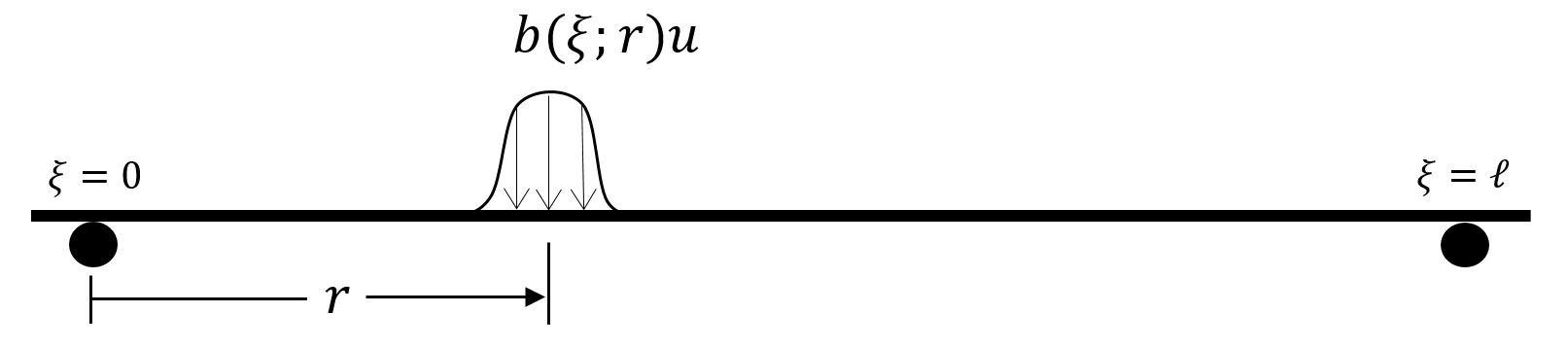
Figure 1: Schematic of an actuator on the railway track beam.

Define the closed self-adjoint positive operator $\mathcal{A}_{0}$ on $L^{2}(0,\ell)$ as:

$$\mathcal{A}_{0}w\coloneqq w_{\xi\xi\xi\xi},$$

(71) $$D(\mathcal{A}_{0})\coloneqq\left\{w\in H^{4}(0,\ell)|\,w(0)=w(\ell)=0,\;w_{\xi\xi}(0)=w_{\xi\xi}(\ell)=0\right\},$$

where the subscript $\cdot_{\xi}$ denote the derivative with respect to the spatial variable. As a result, the state operator associated with the Kelvin-Voigt beam is

(72) $$\mathcal{A}_{\scriptscriptstyle KV}(w,v)\coloneqq\left(v,-\frac{1}{\rho a}\mathcal{A}_{0}(EIw+C_{d}v)\right),$$

which is defined on the state space ${\mathbb{X}}=H^{2}(0,\ell)\cap H_{0}^{1}(0,\ell)\times L^{2}(0,\ell)$ equipped with the norm

(73) $$\|(w,v)\|^{2}=\int_{0}^{\ell}EIw_{\xi\xi}^{2}+kw^{2}+\rho av^{2}\,d\xi.$$

Accordingly, the domain of the state operator is

(74) $$D(\mathcal{A}_{\scriptscriptstyle KV})\coloneqq\left\{(w,v)\in{\mathbb{X}}|\,v\in H^{2}(0,\ell)\cap H_{0}^{1}(0,\ell),\;EIw+C_{d}v\in D(\mathcal{A}_{0})\right\}.$$

The underlying state space ${\mathbb{X}}$ is separable since the spaces $H^{2}(0,\ell)\cap H_{0}^{1}(0,\ell)$ and $L^{2}(0,\ell)$ are separable. Furthermore, define the linear operators $\mathcal{K}$, $\mathcal{B}(r)$, and the nonlinear operator ${\mathcal{F}}(\cdot)$ as

(75) $$\mathcal{K}(w,v)\coloneqq(0,-\frac{1}{\rho a}(\mu v+kw)),$$

(76) $$\mathcal{B}(r)u\coloneqq(0,\frac{1}{\rho a}b(\xi;r)u),$$

(77) $${\mathcal{F}}(w,v)\coloneqq(0,-\frac{\alpha}{\rho a}w^{3}).$$

The operator $\mathcal{K}$ is a bounded linear operator on ${\mathbb{X}}$. For each $r$, operator $\mathcal{B}(r)$ is also a bounded operator that maps an input $u\in\mathbb{R}$ to the state space ${\mathbb{X}}$. Since the space $H^{2}(0,\ell)$ is contained in the space of continuous functions over $[0,\ell]$, the the nonlinear term $w^{3}$ is in $L^{2}(0,\ell)$. Thus, the nonlinear operator ${\mathcal{F}}(\cdot)$ is well-defined on ${\mathbb{X}}$. Lastly, define the operator $\mathcal{A}=\mathcal{A}_{\scriptscriptstyle KV}+\mathcal{K}$, with the same domain as $\mathcal{A}_{\scriptscriptstyle KV}$. With these definition and by setting ${\bm{x}}=(w,v)$, the state space representation of the railway model (6) is

(78) $$\dot{{\bm{x}}}(t)=\mathcal{A}{\bm{x}}(t)+{\mathcal{F}}({\bm{x}}(t))+\mathcal{B}(r)u(t),\quad{\bm{x}}(0)={\bm{x}}_{0}\in D(\mathcal{A}).$$

It is straightforward to show that the operator $\mathcal{A}_{0}$ is closed, densely-defined, self-adjoint, and positive; it also has a compact resolvent. As a result, the operator $\mathcal{A}_{\scriptscriptstyle KV}$ will be a special case of the operator $\mathscr{A}_{B}$ in [12] with $\alpha=1$. According to Theorem 1.1 in [12], such operators are generator of an analytic semigroup (also see [5, Sec. 3] for a different approach). Furthermore, the operator $\mathcal{A}_{\scriptscriptstyle KV}+\mathcal{K}$ is a bounded perturbation of the operator $\mathcal{A}_{\scriptscriptstyle KV}$. By Corollary 3.2.2 in [43], $\mathcal{A}_{\scriptscriptstyle KV}+\mathcal{K}$ also generates an analytic semigroup.

The railway track model in [2] neglects the Kelvin-Voigt damping in the beam (i.e. $C_{d}=0$), and only includes Kelvin-Voigt damping in the ballast. In this case, the semigroup generated by $\mathcal{A}$ is not analytic. The results of this paper hold true for both models.

To guarantee the existence of a unique solution to the PDE (70), the nonlinear operator ${\mathcal{F}}(\cdot)$ needs to fall into assumption A2, B1, C1, and C2. The following result is due to Simon [49, Thm. 3], and will be used to check assumption B1.

Theorem 6.1.

[49, Thm. 3] Let ${\mathbb{X}}$ and $\mathbb{Y}$ be Banach spaces, and $\mathbb{Y}\hookrightarrow{\mathbb{X}}$ with compact embedding. Assume $X\subset L^{p}(0,\tau;{\mathbb{X}})$ where $1\leq p\leq\infty$, and

(79) $$X\text{ is bounded in }L^{1}_{loc}(0,\tau;\mathbb{Y}),$$

(80) $$\int_{0}^{\tau-h}\left\|{\bm{x}}(t+h)-{\bm{x}}(t)\right\|_{{\mathbb{X}}}^{p}dt\to 0\text{ as }h\to 0\text{ uniformly for }{\bm{x}}\in X.$$

Then, $X$ is relatively compact in $L^{p}(0,\tau;{\mathbb{X}})$ (and in $C(0,\tau;{\mathbb{X}})$ if $p=\infty$).

Lemma 6.2.

The operator ${\mathcal{F}}(\cdot)$

1. is continuously Fréchet differentiable on ${\mathbb{X}}$; the Fréchet derivative of this operator at ${\bm{x}}=(w,v)$ maps every ${\bm{p}}=(f,g)$ to ${\mathcal{F}}^{\prime}_{{\bm{x}}}{\bm{p}}=(0,-3\alpha w^{2}f/\rho a)$,

2. the mapping ${\bm{x}}\mapsto{\mathcal{F}}^{\prime}_{{\bm{x}}}$ is bounded, and

3. ${\mathcal{F}}(\cdot)$ satisfies assumption B1.

Proof 6.3.

If ${\mathcal{F}}^{\prime}_{{\bm{x}}}$ is the Fréchet derivative of ${\mathcal{F}}(\cdot)$ at ${\bm{x}}$, this operator must satisfy

(81) $$\lim_{{\bm{p}}\to 0}\frac{\|{\mathcal{F}}({\bm{x}}+{\bm{p}})-{\mathcal{F}}({\bm{x}})-{\mathcal{F}}^{\prime}_{{\bm{x}}}{\bm{p}}\|}{\|{\bm{p}}\|}=0.$$

Recall the definition of the operator ${\mathcal{F}}$ and that of norm on the space ${\mathbb{X}}$, above limit simplifies to

(82) $$\lim_{\|{f}\|_{H^{2}}\to 0}\frac{\|{f}^{3}+3{f}^{2}{w}\|_{L^{2}}}{\|{f}\|_{H^{2}}}=0.$$

Notice that functions $f$ and $w$ are in $H^{2}(0,\ell)$, and thus, continuous on $[0,\ell]$. Use triangle inequality, and Hölder’s inequality to obtain

$$\|{f}^{3}+3{f}^{2}{w}\|_{L^{2}} \leq\|{f}^{3}\|_{L^{2}}+\|3{f}^{2}{w}\|_{L^{2}}$$

(83) $$\leq\|{f}\|_{L^{6}}^{3}+3\|{f}\|_{L^{8}}^{2}\|{w}\|_{L^{4}}.$$

Apply the Sobolev embedding result $H^{2}(0,\ell)\hookrightarrow L^{p}(0,\ell)$ and let $c_{p}$ be the embedding constant

(84) $$\|{f}^{3}+3{f}^{2}{w}\|_{L^{2}} \leq c_{6}^{3}\|{f}\|_{H^{2}}^{3}+3c_{8}^{2}c_{4}\|{f}\|_{H^{2}}^{2}\|{w}\|_{H^{2}},$$

As a result, the expression in (82) is bounded above according to

(85) $$\frac{\|{f}^{3}+3{f}^{2}{w}\|_{L^{2}}}{\|{f}\|_{H^{2}}}\leq c_{6}^{3}\|f\|^{2}_{H^{2}}+3c_{8}^{2}c_{4}\|w\|_{H^{2}}\|f\|_{H^{2}}.$$

This shows that the limit in (82) holds, and the operator ${\mathcal{F}}(\cdot)$ is indeed Fréchet differentiable.

Furthermore, select ${\bm{x}}_{1}=(w_{1},v_{1})$, ${\bm{x}}_{2}=(w_{2},v_{2})$, and ${\bm{p}}=(f,g)$ as generic elements of ${\mathbb{X}}$. The Fréchet derivative of ${\mathcal{F}}(\cdot)$ at ${\bm{x}}_{2}-{\bm{x}}_{1}$ is

$${\mathcal{F}}^{\prime}_{{\bm{x}}_{2}-{\bm{x}}_{1}}{\bm{p}}=(0,-\frac{3\alpha}{\rho a}(w_{2}-w_{1})^{2}f).$$

Take the norm of ${\mathcal{F}}^{\prime}_{{\bm{x}}_{2}-{\bm{x}}_{1}}{\bm{p}}$, and use Hölder’s inequality to obtain

$$\left\|{\mathcal{F}}^{\prime}_{{\bm{x}}_{2}-{\bm{x}}_{1}}{\bm{p}}\right\| =\frac{3\alpha}{\sqrt{\rho a}}\left(\int_{0}^{\ell}(w_{2}(\xi)-w_{1}(\xi))^{4}f^{2}(\xi)\,d\xi\right)^{\frac{1}{2}}$$

(86) $$\leq\frac{3\alpha}{\sqrt{\rho a}}\left\|w_{2}-w_{1}\right\|_{L^{8}}^{2}\left\|f\right\|_{L^{4}}.$$

Applying the Sobolev embedding result $H^{2}(0,\ell)\hookrightarrow L^{p}(0,\ell)$ yields

$$\left\|{\mathcal{F}}^{\prime}_{{\bm{x}}_{2}-{\bm{x}}_{1}}{\bm{p}}\right\| \leq\frac{3\alpha}{\sqrt{\rho a}}c_{8}^{2}c_{4}\left\|w_{2}-w_{1}\right\|_{H^{2}}^{2}\left\|f\right\|_{H^{2}}$$

(87) $$\leq\frac{3\alpha}{\sqrt{\rho a}}c_{8}^{2}c_{4}\left\|{\bm{x}}_{2}-{\bm{x}}_{1}\right\|^{2}\left\|{\bm{p}}\right\|.$$

The last inequality indicates that the operator norm of ${\mathcal{F}}^{\prime}_{{\bm{x}}}$ continuously depends on ${\bm{x}}$.

Inequality (87) also yields

(88) $$\left\|{\mathcal{F}}^{\prime}_{{\bm{x}}}\right\|_{\mathcal{L}({\mathbb{X}})}\leq\frac{3\alpha}{\sqrt{\rho a}}c_{8}^{2}c_{4}\left\|{\bm{x}}\right\|^{2}.$$

This shows that the mapping ${\bm{x}}\mapsto{\mathcal{F}}^{\prime}_{{\bm{x}}}$ is bounded.

To show that the nonlinear operator ${\mathcal{F}}(\cdot)$ satisfies assumption B1, consider a bounded sequence ${\bm{x}}_{n}(t)=(w_{n}(t),v_{n}(t))$ in $C(0,\tau;{\mathbb{X}})$ weakly converging to some element ${\bm{x}}(t)=(w(t),v(t))$ in $L^{p}(0,\tau;{\mathbb{X}})$. It is shown that the sequence $w_{n}(t)$ satisfies conditions of Theorem 6.1. The sequence $w_{n}(t)$ is by assumption bounded in $C(0,\tau;H^{2}(0,\ell)\cap H^{1}_{0}(0,\ell))$, and so in $C(0,\tau;L^{6}(0,\ell))$. This ensures that for all $p\in[1,\infty)$

(89) $$\int_{0}^{\tau-h}\left\|w_{n}(t+h)-w_{n}(t)\right\|_{L^{6}(0,\ell)}^{p}dt\to 0\text{ as }h\to 0\text{ uniformly for all }n.$$

Also, the space $H^{2}(0,\ell)\cap H^{1}_{0}(0,\ell)$ is compactly embedded in $L^{6}(0,\ell)$ by Rellich-Kondrachov compact embedding theorem [1, Ch. 6]. According to Theorem 6.1, $w_{n}(t)$ has a strongly convergent subsequence in $L^{p}(0,\tau;L^{6}(0,\ell))$. Recall that $w_{n}(t)$ weakly converges to $w(t)$ in $L^{2}(0,\tau;H^{2}(0,\ell)\cap H^{1}_{0}(0,\ell))$ as well. A weak limit is unique; thus, $w_{n}\to w$ in $L^{p}(0,\tau;L^{6}(0,\ell))$. This further implies that $w_{n}^{3}\to w^{3}$ in $L^{p}(0,\tau;L^{2}(0,\ell))$. The nonlinear operator ${\mathcal{F}}(\cdot)$ maps ${\bm{x}}_{n}(t)$ to

(90) $${\mathcal{F}}(w_{n}(t),v_{n}(t))=(0,\frac{\alpha}{\rho a}w_{n}^{3}(t)).$$

Thus, the sequence ${\mathcal{F}}(w_{n}(t),v_{n}(t))$ strongly (and so weakly) converges to ${\mathcal{F}}(w(t),v(t))$ in $L^{2}(0,\tau;{\mathbb{X}})$.

The previous lemma ensures that the nonlinear operator ${\mathcal{F}}(\cdot)$ satisfies assumption A2. By Theorem 3.1, for control inputs $u\in L^{p}(0,\tau)$, $1<p<\infty$, the existence of a unique local mild solution is guaranteed.

To address the optimization problem P for the railway track model, assumption B and C need to be satisfied. In Lemma 5.8, it was shown that assumption B3 will hold for the particular choice of the cost function in assumption C3. As a result, the existence of an optimal pair $(u^{o},r^{o})$ together with an optimal trajectory ${\bm{x}}^{o}$ follows from Theorem 4.1.

Accordingly, using Theorem 5.10, the optimal pair $(u^{o},r^{o})$ satisfies the equation (62). In order to characterize the optimizers (62) some adjoint operators need to be calculated. Calculation of the operator $\mathcal{A}^{*}$ is straightforward; it is

(91) $$\mathcal{A}^{*}(f,g)=\left(-g,\frac{1}{\rho a}\mathcal{A}_{0}(EIf-C_{d}g)+\frac{k}{\rho a}f-\frac{\mu}{\rho a}g\right),\$$

for all $(f,g)$ in the domain

(92) $$D(\mathcal{A}^{*})=\left\{(f,g)\in{\mathbb{X}}|\,g\in H^{2}(0,\ell)\cap H_{0}^{1}(0,\ell),\;EIf-C_{d}g\in D(\mathcal{A}_{0})\right\}.$$

Let ${\bm{x}}^{o}(t)=(w^{o},v^{o})$ be the optimal trajectory evaluated at time $t\in[0,\tau]$. To calculate the adjoint of the operator ${\mathcal{F}}^{\prime}_{{\bm{x}}^{o}(t)}$ for every $t\in[0,\tau]$ on ${\mathbb{X}}$, take the inner product ${\mathcal{F}}^{\prime}_{{\bm{x}}^{o}(t)}(w,v)$ with $(f,g)\in{\mathbb{X}}$; that is

(93) $$\left\langle{\mathcal{F}}^{\prime}_{{\bm{x}}^{o}(t)}(w,v),(f,g)\right\rangle=\int_{0}^{\ell}-{3\alpha}(w^{o}(\xi))^{2}w(\xi)g(\xi)\,d\xi.$$

For any $g\in L^{2}(0,\ell)$, consider the function $h\in H^{2}(0,\ell)\cap H^{1}_{0}(0,\ell)$ satisfying the differential equation

$$EIh_{\xi\xi\xi\xi}(\xi)+kh(\xi)=-{3\alpha}(w^{o}(\xi))^{2}g(\xi),$$

$$h(0)=h(\ell)=0,$$

(94) $$h_{\xi\xi}(0)=h_{\xi\xi}(\ell)=0.$$

An explicit solution $h(\xi)$ to (6) can be calculated using a Green’s function:

$$h(\xi) =-{3\alpha}\int_{0}^{\ell}G(\xi,{\eta})(w^{o}({\eta}))^{2}g({\eta})\,d{\eta},$$

(97) $$G(\xi,{\eta}) =\frac{1}{6\ell}\left\{\begin{array}[]{ll}(2\ell^{2}{\eta}-3\ell{\eta}^{2}+{\eta}^{3})\xi+({\eta}-\ell)\xi^{3},\quad\xi\leq{\eta}\\ ({\eta}^{3}-\ell^{2}{\eta})\xi+{\eta}\xi^{3},\quad\xi>{\eta}\,.\\ \end{array}\right.$$

With this calculation, for any $(w,v)\in{\mathbb{X}},$

$$\left\langle(w,v),(h,0)\right\rangle =\int_{0}^{\ell}EIw_{\xi\xi}(\xi)h_{\xi\xi}(\xi)+kw(\xi)h(\xi)\,d\xi$$

$$=EI[h_{\xi\xi}w_{\xi}]_{0}^{\ell}-EI[h_{\xi\xi\xi}w]_{0}^{\ell}+\int_{0}^{\ell}(EIh_{\xi\xi\xi\xi}(\xi)+kh(\xi))w(\xi)\,d\xi$$

(98) $$=\int_{0}^{\ell}-{3\alpha}(w^{o}(\xi))^{2}w(\xi)g(\xi)\,d\xi.$$

Comparing this equation to (93); the adjoint of ${\mathcal{F}}^{\prime}_{{\bm{x}}^{o}(t)}$ is defined by

(99) $${\mathcal{F}}^{\prime*}_{{\bm{x}}^{o}(t)}(f,g)=(h,0).$$

The adjoint of the operator $\mathcal{B}(r)$ for every $(f,g)\in{\mathbb{X}}$ is

(100) $$\mathcal{B}^{*}(r)(f,g)=\int_{0}^{\ell}b(\xi;r)g(\xi)\,d\xi.$$

Also, denote $b_{r}(\xi;r)$ to be the derivative of $b(\xi;r)$ with respect to $r$ and let ${\bm{p}}^{o}(t)=(f,g)$ at time $t\in[0,\tau]$. Use Corollary 5.13 to find

(101) $$({\mathcal{B}}^{\prime}_{r}u)^{*}{\bm{p}}^{o}(t)=u\int_{0}^{\ell}b_{r}(\xi;r)g(\xi)d\xi,\quad\forall(f,g)\in{\mathbb{X}}.$$

Furthermore, let $q_{1}\in C^{2}([0,\ell])$ and $q_{2}\in C([0,\ell])$ be some non-negative functions. Set $\mathcal{Q}(w,v)=(q_{1}w,q_{2}v)$ and $\mathcal{R}=1$ in the cost function of assumption C3.

In conclusion, assuming that $(u^{o},r^{o})$ is in the interior of $U_{ad}\times K_{ad}$, the following set of equations yields an optimizer for every initial condition ${\bm{x}}_{0}=(w_{0},v_{0})\in{\mathbb{X}}$:

(IVP) $$\begin{cases}\rho aw^{o}_{tt}+(EIw^{o}_{\xi\xi}+C_{d}w^{o}_{t\xi\xi})_{\xi\xi}+\mu w^{o}_{t}+kw^{o}+\alpha(w^{o})^{3}=b(\xi;r^{o})u^{o}(t),\\ w^{o}(0,t)=w^{o}(\ell,t)=0,\\ EIw^{o}_{\xi\xi}(0,t)+C_{d}w^{o}_{t\xi\xi}(0,t)=EIw^{o}_{\xi\xi}(\ell,t)+C_{d}w^{o}_{t\xi\xi}(\ell,t)=0\\ w^{o}(\xi,0)=w_{0}(\xi),\;w^{o}_{t}(\xi,0)=v_{0}(\xi),\end{cases}$$

(FVP) $$\begin{cases}\rho af^{o}_{t}-\rho ag^{o}+3\alpha\int_{0}^{\ell}G(\xi,{\eta})(w^{o}({\eta}))^{2}g^{o}({\eta})\,d{\eta}=-\rho aq_{1}(\xi)w^{o},\\ \rho ag^{o}_{t}+(EIf^{o}_{\xi\xi}-C_{d}g^{o}_{\xi\xi})_{\xi\xi}-\mu g^{o}+kf^{o}=-\rho aq_{2}(\xi)w^{o}_{t},\\ f^{o}(0,t)=f^{o}(\ell,t)=0,\;g^{o}(0,t)=g^{o}(\ell,t)=0,\\ EIf^{o}_{\xi\xi}(0,t)-C_{d}g^{o}_{\xi\xi}(0,t)=EIf^{o}_{\xi\xi}(\ell,t)-C_{d}g^{o}_{\xi\xi}(\ell,t)=0\\ f^{o}(\xi,T)=0,\;g^{o}(\xi,T)=0,\end{cases}$$

(OPT) $$\begin{cases}u^{o}(t)=-\int_{0}^{\ell}b(\xi;r^{o})g^{o}(\xi,t)\,d\xi,\\ \int_{0}^{\tau}\int_{0}^{\ell}u^{o}(t)b_{r}(\xi;r^{o})g^{o}(\xi,t)\,d\xi dt=0.\end{cases}$$

7 Nonlinear Waves

Nonlinear waves occur in many applications, including fluid mechanics, electromagnetism, elasticity, and also relativistic quantum mechanics. Let the wave evolve on a region $\Omega$ that is a bounded, open, connected subset of $\mathbb{R}^{2}$. It is assumed that $\Omega$ has a Lipschitz boundary separated into $\partial\Omega=\overline{\Gamma_{0}\cup\Gamma_{1}}$ where $\Gamma_{0}\cap\Gamma_{1}=\emptyset$ and $\Gamma_{0}\neq\emptyset$. Denote by $\nu$ the unit outward normal vector field on $\partial\Omega$. Figure 2 illustrates the region and the shape of an actuator. Define ${\mathbb{K}}=L^{2}(\Omega)$ and let $r(\xi)$, $\xi\in\Omega$, be the actuator shape design. There are many possible choices of admissible shapes. One is

$$K_{ad}=\{r\in C^{1}(\overline{\Omega}):\left\|r\right\|_{C^{1}(\overline{\Omega})}\leq 1\}.$$

A nonlinear wave model with initial conditions $w_{0}(\xi)$ and $v_{0}(\xi)$ is

$$\begin{cases}\begin{aligned} &\frac{\partial^{2}w}{\partial t^{2}}(\xi,t)=\Delta w(\xi,t)+F(w(\xi,t))+r(\xi)u(t),&(\xi,t)&\in\Omega\times(0,\infty),\\ &w(\xi,0)=w_{0}(\xi),\;\frac{\partial w}{\partial t}(\xi,0)=v_{0}(\xi),&\xi&\in\Omega,\\ &w(\xi,t)=0,&(\xi,t)&\in\Gamma_{0}\times[0,\infty),\\ &\frac{\partial w}{\partial\nu}(\xi,t)=0,&(\xi,t)&\in\Gamma_{1}\times[0,\infty).\end{aligned}\end{cases}$$

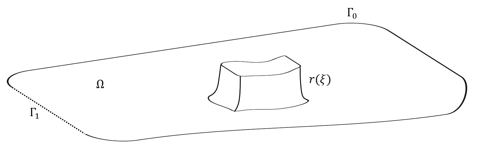
Figure 2: Schematic of an actuator on the wave region.

Let ${\mathbb{X}}=H^{1}_{\Gamma_{0}}(\Omega)\times L^{2}(\Omega)$ and define ${\mathcal{A}}:D({\mathcal{A}})\to{\mathbb{X}}$ as

(102) $${\mathcal{A}}(w,v)=(v,\nabla w),$$

$$D({\mathcal{A}})=\left\{(w,v)\in{\mathbb{X}}\,|\,w\in H^{2}(\Omega)\cap H_{\Gamma_{0}}^{1}(\Omega),\;v\in H^{1}_{\Gamma_{0}}(\Omega),\;\frac{\partial w}{\partial\nu}{\Big{|}}_{\Gamma_{1}}=0\right\}.$$

The operator ${\mathcal{A}}$ is skew-adjoint and generates a strongly continuous unitary group on ${\mathbb{X}}$; see for example, [18, Thm. 3.24].

Assumption D.

1. The function $F(\zeta)$ is twice continuously differentiable over $\mathbb{R}$; denote its derivatives by $F^{\prime}(\zeta)$ and $F^{\prime\prime}(\zeta)$.

2. There are numbers $a_{0}>0$ and $b>1/2$ such that $|F^{\prime\prime}(\zeta)|\leq a_{0}(1+|\zeta|^{b})$.

The nonlinear operator ${\mathcal{F}}(\cdot):{\mathbb{X}}\to{\mathbb{X}}$ is defined as

(103) $${\mathcal{F}}(w,v)=(0,F(w)).$$

Assumption D is needed to ensure that ${\mathcal{F}}(\cdot):{\mathbb{X}}\to{\mathbb{X}}$ and satisfies assumption B1 and that the Gâteaux derivative of ${\mathcal{F}}(\cdot)$ is also an operator on ${\mathbb{X}}$. Some examples of $F(\cdot)$ satisfying this assumption are $F(w)=\sin(w)$ in the Sine-Gordon equation and $F(w)=|w|^{k}w,\;k\geq 2$ in the Klein-Gordon equation [48, Sec. 5.2].

Lemma 7.1.

Under assumption D,

1. the operator ${\mathcal{F}}(\cdot)$ is Gâteaux differentiable on ${\mathbb{X}}$, with the Gâteaux derivative at ${\bm{x}}=(w,v)$ in the direction ${\bm{p}}=(f,g)$ given by ${\mathcal{F}}^{\prime}_{{\bm{x}}}{\bm{p}}=(0,F^{\prime}(w)f)$,

2. the mapping ${\bm{x}}\mapsto{\mathcal{F}}^{\prime}_{{\bm{x}}}$ is bounded, and

3. ${\mathcal{F}}(\cdot)$ satisfies assumption B1.

Proof 7.2.

To prove the first part of the lemma, it must be shown that for any variation $f\in H^{1}_{\Gamma_{0}}(\Omega),$

(104) $$\lim_{\epsilon\to 0}\left\|\frac{1}{\epsilon}\left(F(w+\epsilon f)-F(w)\right)-F^{\prime}(w)f\right\|_{L^{2}(\Omega)}=0,$$

or

(105) $$\lim_{\epsilon\to 0}\int_{\Omega}{\big{|}}\frac{1}{\epsilon}\left(F(w(\xi)+\epsilon f(\xi))-F(w(\xi))\right)-F^{\prime}(w(\xi))f(\xi){\big{|}}^{2}\,d\xi=0.$$

Recall that because of the continuous embedding $H^{1}_{\Gamma_{0}}(\Omega)\hookrightarrow L^{p}(\Omega)$, the functions $f$ and $w$ belong to $L^{p}(\Omega)$ for all $p\in[1,\infty)$. Use of assumption D, applying Taylor’s theorem with integral reminder to $F(\cdot)$, and using Jensen’s inequality, the integral in (105) becomes

$$\int_{\Omega}\left(\int_{0}^{1}\epsilon(1-\eta)F^{\prime\prime}(w(\xi)+\eta\epsilon f(\xi))f^{2}(\xi)d\eta\right)^{2}d\xi$$

$$\leq\int_{\Omega}\int_{0}^{1}\epsilon^{2}(1-\eta)^{2}F^{\prime\prime 2}(w(\xi)+\eta\epsilon f(\xi))f^{4}(\xi)d\eta d\xi$$

(106) $$\leq\int_{\Omega}\int_{0}^{1}\epsilon^{2}(1-\eta)^{2}a_{0}^{2}\left(2+2^{2b}|w(\xi)|^{2b}+2^{2b}\eta^{2b}|\epsilon|^{2b}|f(\xi)|^{2b}\right)f^{4}(\xi)d\eta d\xi$$

Applying Hölder’s inequality shows that integral (106) is bounded above by a number, and also converges to zero as $\epsilon\to 0$.

Furthermore, the operator ${\mathcal{F}}^{\prime}_{{\bm{x}}}$ satisfies, for any ${\bm{x}}=(w,v)$ and ${\bm{p}}=(f,g)$ in ${\mathbb{X}}$,

(107) $$\left\|{\mathcal{F}}^{\prime}_{{\bm{x}}}{\bm{p}}\right\|^{2}=\int_{\Omega}F^{\prime 2}(w(\xi))f^{2}(\xi)d\xi.$$

Assumption D1 ensures that there is a number $a_{1}>0$ such that $|F^{\prime}(\zeta)|\leq a_{1}(1+|\zeta|^{b+1})$. Use this together with Hölder’s inequality to obtain

$$\left\|{\mathcal{F}}^{\prime}_{{\bm{x}}}{\bm{p}}\right\|^{2} \leq\int_{\Omega}2a_{1}^{2}(1+w^{2b+2}(\xi))f^{2}(\xi)d\xi.$$

(108) $$\leq 2a^{2}_{1}\left(\left\|f\right\|_{L^{2}(\Omega)}^{2}+\left\|w\right\|_{L^{4b+4}(\Omega)}^{2b+2}\left\|f\right\|_{L^{4}(\Omega)}^{2}\right)$$

Apply the embeddings $H^{1}_{\Gamma_{0}}(\Omega)\hookrightarrow L^{p}(\Omega)$; letting $c_{p}$ indicates the various embedding constants,

$$\left\|{\mathcal{F}}^{\prime}_{{\bm{x}}}{\bm{p}}\right\|^{2} \leq 2a^{2}_{1}\left(c^{2}_{2}+c_{4b+4}^{2b+2}c_{4}^{2}\left\|w\right\|_{H^{1}_{\Gamma_{0}}(\Omega)}^{2b}\right)\left\|f\right\|_{H^{1}_{\Gamma_{0}}(\Omega)}^{2}$$

(109) $$\leq 2a^{2}_{1}\left(c^{2}_{2}+c_{4b+4}^{2b+2}c_{4}^{2}\left\|{\bm{x}}\right\|^{2b}\right)\left\|{\bm{p}}\right\|^{2}.$$

Inequality (109) implies that

(110) $$\left\|{\mathcal{F}}^{\prime}_{{\bm{x}}}\right\|_{\mathcal{L}({\mathbb{X}})}^{2}\leq 2a^{2}_{1}\left(c^{2}_{2}+c_{4b+4}^{2b+2}c_{4}^{2}\left\|{\bm{x}}\right\|^{2b}\right).$$

This inequality shows that the mapping ${\bm{x}}\mapsto{\mathcal{F}}^{\prime}_{{\bm{x}}}$ is bounded.

It will now be shown that ${\mathcal{F}}(\cdot)$ satisfies assumption B1. Consider a bounded sequence ${\bm{x}}_{n}(t)=(w_{n}(t),v_{n}(t))$ in $C(0,\tau;{\mathbb{X}})$ that weakly converges to some element ${\bm{x}}(t)=(w(t),v(t))$ in $L^{p}(0,\tau;{\mathbb{X}})$. The sequence $w_{n}(t)$ is bounded in $C(0,\tau;H^{1}_{\Gamma_{0}}(\Omega))$ and so it is in $C(0,\tau;L^{q}(\Omega))$ for all $q\in[1,\infty)$. This together with the bounded convergence theorem ensures that for every $p\in[1,\infty)$

(111) $$\int_{0}^{\tau-h}\left\|w_{n}(t+h)-w_{n}(t)\right\|_{L^{q}(\Omega)}^{p}dt\to 0\text{ as }h\to 0\text{ uniformly for all }n.$$

The space $H^{1}_{\Gamma_{0}}(\Omega)$ is compactly embedded in $L^{q}(\Omega)$ by Rellich-Kondrachov compact embedding theorem [1, Ch. 6]. By Theorem 6.1, this embedding together with (111) ensures that $w_{n}(t)$ has a strongly convergent subsequence in $L^{p}(0,\tau;L^{q}(\Omega))$. The sequence $w_{n}(t)$ by assumption converges weakly to $w(t)$ in $L^{p}(0,\tau;H^{1}_{\Gamma_{0}}(\Omega))$; a weak limit is unique, so $w_{n}(t)$ converges strongly to $w(t)$ in $L^{p}(0,\tau;L^{q}(\Omega))$. The nonlinear operator ${\mathcal{F}}(\cdot)$ maps ${\bm{x}}_{n}(t)$ to

(112) $${\mathcal{F}}(w_{n}(t),v_{n}(t))=(0,F(w_{n}(t))).$$

Use Taylor’s theorem with integral reminder, and let $h(\xi,t;\eta)=w(\xi,t)+\eta(w_{n}(\xi,t)-w(\xi,t))$, $\eta\in[0,1]$, to obtain

(113) $$|F(w_{n}(\xi,t))-F(w(\xi,t))| \leq\left(\int_{0}^{1}|F^{\prime}(h(\xi,t;\eta))|d\eta\right)|w_{n}(\xi,t)-w(\xi,t)|.$$

Let

$$M_{1}(\xi,t)=a_{1}\left(1+\int_{0}^{1}|h(\xi,t;\eta)|^{b+1}d\eta\right).$$

Taking integral of both side of (113) and using Hölder inequality yield

$$\left\|F(w_{n})-F(w)\right\|_{L^{p}(0,\tau;L^{2}(\Omega))}^{p} \leq\int_{0}^{\tau}\left(\int_{\Omega}M_{1}^{2}(\xi,t)|w_{n}(\xi,t)-w(\xi,t)|^{2}d\xi\right)^{\frac{p}{2}}dt$$

(114) $$\leq\left\|M_{1}\right\|_{L^{2p}(0,\tau;L^{4}(\Omega))}^{p}\left\|w_{n}-w\right\|_{L^{2p}(0,\tau;L^{4}(\Omega))}^{p}.$$

Note that $\left\|M_{1}\right\|_{L^{2p}(0,\tau;L^{4}(\Omega))}<\infty$ since $w(\xi,t)$ and $w_{n}(\xi,t)$ are in $L^{p}(0,\tau;L^{q}(\Omega))$ for all $p\in[1,\infty)$ and $q\in[1,\infty)$. From (114), it follows that $F(w_{n})$ strongly converges to $F(w)$ in $L^{p}(0,\tau;L^{2}(\Omega))$. Therefore, the sequence ${\mathcal{F}}(w_{n}(t),v_{n}(t))$ strongly (and so weakly) converges to ${\mathcal{F}}(w(t),v(t))$ in $L^{p}(0,\tau;{\mathbb{X}})$.

Let ${\bm{x}}^{o}(t)=(w^{o},v^{o})$ at time $t\in[0,\tau]$. As for the railway track example, in order to obtain an expression for the adjoint of the operator ${\mathcal{F}}^{\prime}_{{\bm{x}}^{o}(t)}$, the following boundary-value problem needs to be solved:

(115) $$\begin{cases}\begin{aligned} &\Delta h(\xi)=-F^{\prime}(w^{o}(\xi))g(\xi),\quad&\xi&\in\Omega,\\ &h(\xi)=0,\quad&\xi&\in\Gamma_{0},\\ &\frac{\partial h}{\partial\nu}(\xi)=0,\quad&\xi&\in\Gamma_{1}.\end{aligned}\end{cases}$$

The adjoint with respect to ${\mathbb{X}}$ of ${\mathcal{F}}^{\prime}_{{\bm{x}}^{o}(t)}$ is

(116) $${\mathcal{F}}^{\prime*}_{{\bm{x}}^{o}(t)}(f,g)=(h,0),$$

where $h$ solves (115). Define ${\mathbb{U}}=\mathbb{R}$ and the input operator ${\mathcal{B}}(r)\in\mathcal{L}({\mathbb{U}},{\mathbb{X}})$ by

(117) $${\mathcal{B}}(r)u=(0,r(\xi)u).$$

The adjoint of this operator is

(118) $${\mathcal{B}}^{*}(r)(f,g)=\int_{\Omega}r(\xi)g(\xi)d\xi,\quad\forall(f,g)\in{\mathbb{X}}.$$

Let ${\bm{p}}^{o}(t)=(f,g)$ at time $t\in[0,\tau]$. Use Corollary 5.13 to find

(119) $$({\mathcal{B}}^{\prime}_{r}u)^{*}{\bm{p}}^{o}(t)=ug.$$

Furthermore, let $q_{1}\in C^{1}(\overline{\Omega})$ and $q_{2}\in C(\overline{\Omega})$ be some non-negative functions. Set $\mathcal{Q}(w,v)=(q_{1}w,q_{2}v)$ and $\mathcal{R}=1$ in the cost function of assumption C3.

If the optimal control $u^{o}$ and optimal actuator design $r^{o}$ are in the interior of $U_{ad}\times K_{ad}$, then by Corollary 5.13 the following equations are satisfied:

(IVP) $$\begin{cases}\begin{aligned} &\frac{\partial^{2}w^{o}}{\partial t^{2}}(\xi,t)=\Delta w^{o}(\xi,t)+F(w^{o}(\xi,t))+r^{o}(\xi)u^{o}(t),&(\xi,t)&\in\Omega\times(0,\tau],\\ &w^{o}(\xi,0)=w_{0}(\xi),\;\frac{\partial w^{o}}{\partial t}(\xi,0)=v_{0}(\xi),&\xi&\in\Omega,\\ &w^{o}(\xi,t)=0,&(\xi,t)&\in\Gamma_{0}\times[0,\tau],\\ &\frac{\partial w^{o}}{\partial\nu}(\xi,t)=0,&(\xi,t)&\in\Gamma_{1}\times[0,\tau],\end{aligned}\end{cases}$$

(FVP) $$\begin{cases}\begin{aligned} &\frac{\partial f^{o}}{\partial t}(\xi,t)=-g^{o}(\xi,t)-h^{o}(\xi,t)-q_{1}(\xi)w^{o}(\xi,t),&(\xi,t)&\in\Omega\times(0,\tau],\\[2.84526pt] &\frac{\partial g^{o}}{\partial t}(\xi,t)=-\Delta f^{o}(\xi,t)-q_{2}(\xi)\frac{\partial w^{o}}{\partial t}(\xi,t),&(\xi,t)&\in\Omega\times(0,\tau],\\[2.84526pt] &f^{o}(\xi,\tau)=0,\;g^{o}(\xi,\tau)=0,&\xi&\in\Omega,\\[2.84526pt] &f^{o}(\xi,t)=0,&(\xi,t)&\in\Gamma_{0}\times[0,\tau],\\[2.84526pt] &\frac{\partial f^{o}}{\partial\nu}(\xi,t)=0,&(\xi,t)&\in\Gamma_{1}\times[0,\tau],\end{aligned}\end{cases}$$

(OPT) $$\begin{cases}\begin{aligned} &u^{o}(t)=-\int_{\Omega}r^{o}(\xi)g^{o}(\xi,t)d\xi,&t&\in[0,\tau],\\ &\int_{0}^{\tau}u^{o}(t)g^{o}(\xi,t)dt=0,&\xi&\in\Omega.\end{aligned}\end{cases}$$

8 Conclusions

Optimal control of semi-linear infinite-dimensional systems was considered in this paper where the optimal controller design involves both the controlled input and the actuator design. It was shown that the existence of an optimal control together with an optimal actuator design is guaranteed under some assumptions. Moreover, first-order necessary optimality conditions were obtained. The theory was illustrated with several applications.

Current work is concerned with developing numerical methods for solution of the optimality equations and also the consideration of a wider class of nonlinearities. Extension of these problems to situations where the input operator is not bounded on the state space is also of interest.

Appendix A Proof of Proposition 5.2

For ${\bm{x}}_{0}\in{\mathbb{X}}$ and ${\bm{r}}\in K_{ad}$, consider ${\bm{x}}_{1}(t)$ and ${\bm{x}}_{2}(t)$ as the mild solutions to (1) corresponding to the inputs ${\bm{u}}_{1}(t)$ and ${\bm{u}}_{2}(t)$, respectively. The inputs are in a ball of radius $R$ contained in $L^{p}(0,\tau;{\mathbb{U}})$, $1<p<\infty$; consequently, by Corollary 3.3 and assumption A3, the states ${\bm{x}}_{1}(t)$ and ${\bm{x}}_{2}(t)$ are contained in a ball of radius

(A.1) $$\delta=c_{\tau}(\left\|{\bm{x}}_{0}\right\|+M_{\mathcal{B}}R).$$

From (2), it follows that

$${\bm{x}}_{2}(t)-{\bm{x}}_{1}(t)= \int_{0}^{t}\mathcal{T}(t-s)\left({\mathcal{F}}({\bm{x}}_{2}(s))-{\mathcal{F}}({\bm{x}}_{1}(s))\right)ds$$

(A.2) $$+\int_{0}^{t}\mathcal{T}(t-s)\mathcal{B}({\bm{r}})\left({\bm{u}}_{2}(s)-{\bm{u}}_{1}(s)\right)ds.$$

Recall that $\mathcal{T}(t)$ satisfies $\left\|\mathcal{T}(t)\right\|\leq M_{{\mathcal{T}}}$ for all $t\in[0,\tau]$ and some number $M_{{\mathcal{T}}}>0$. Also, remember that the operator ${\mathcal{F}}(\cdot)$ is locally Lipschitz continuous, and $\mathcal{B}({\bm{r}})$ is uniformly bounded in ${\mathbb{X}}$ for all ${\bm{r}}\in K_{ad}$. Taking the norm in ${\mathbb{X}}$ of both sides of this equation yields

$$\left\|{\bm{x}}_{2}(t)-{\bm{x}}_{1}(t)\right\|\leq M_{{\mathcal{T}}}L_{{\mathcal{F}}\delta}\int_{0}^{t}\left\|{\bm{x}}_{2}(s)-{\bm{x}}_{1}(s)\right\|\,ds$$

(A.3) $$+M_{{\mathcal{T}}}M_{\mathcal{B}}\tau^{(p-1)/p}\left\|{\bm{u}}_{2}-{\bm{u}}_{1}\right\|_{p}.$$

Define the constant $L_{{\bm{u}}}$ as

(A.4) $$L_{{\bm{u}}}=e^{M_{{\mathcal{T}}}L_{{\mathcal{F}}\delta}\tau}M_{{\mathcal{T}}}M_{\mathcal{B}}\tau^{(p-1)/p}.$$

By Gronwall’s Lemma [57, Thm. 1.4.1], it follows that

(A.5) $$\left\|{\bm{x}}_{2}-{\bm{x}}_{1}\right\|_{C(0,\tau;{\mathbb{X}})}\leq L_{{\bm{u}}}\left\|{\bm{u}}_{2}-{\bm{u}}_{1}\right\|_{p}.$$

This is in fact the inequality (28).

Similarly, for a fixed initial condition ${\bm{x}}_{0}\in{\mathbb{X}}$ and control input ${\bm{u}}\in U_{ad}$, consider ${\bm{x}}_{1}(t)$ and ${\bm{x}}_{2}(t)$ as the mild solutions to (1) corresponding to the actuator designs ${\bm{r}}_{1}$ and ${\bm{r}}_{2}$, respectively. Use local Lipschitz continuity of ${\mathcal{F}}(\cdot)$ and growth condition on semigroup $\mathcal{T}(t)$ and obtain

$$\left\|{\bm{x}}_{2}(t)-{\bm{x}}_{1}(t)\right\|\leq M_{{\mathcal{T}}}L_{{\mathcal{F}}\delta}\int_{0}^{t}\left\|{\bm{x}}_{2}(s)-{\bm{x}}_{1}(s)\right\|\,ds$$

(A.6) $$+M_{{\mathcal{T}}}\tau^{(p-1)/p}\left\|{\bm{u}}\right\|_{p}\left\|\mathcal{B}({\bm{r}}_{2})-\mathcal{B}({\bm{r}}_{1})\right\|_{\mathcal{L}({\mathbb{U}},{\mathbb{X}})}.$$

Assumption C2 implies that the control operator $\mathcal{B}({\bm{r}})$ is locally Lipschitz continuous with respect to ${\bm{r}}$. That is, letting

$$L_{\mathcal{B}}=\sup\{\left\|{\mathcal{B}}^{\prime}_{\bm{r}}\right\|_{\mathcal{L}({\mathbb{K}},\mathcal{L}({\mathbb{U}},{\mathbb{X}}))}:{\bm{r}}\in K_{ad}\},$$

operator ${\mathcal{B}}({\bm{r}})$ for all ${\bm{r}}_{1}$ and ${\bm{r}}_{2}$ in $K_{ad}$ satisfies

(A.7) $$\left\|\mathcal{B}({\bm{r}}_{2})-\mathcal{B}({\bm{r}}_{1})\right\|_{\mathcal{L}({\mathbb{U}},{\mathbb{X}})}\leq L_{\mathcal{B}}\left\|{\bm{r}}_{2}-{\bm{r}}_{1}\right\|_{\mathbb{K}}.$$

Accordingly, the inequality (A) can be re-written as

$$\left\|{\bm{x}}_{2}(t)-{\bm{x}}_{1}(t)\right\|\leq M_{{\mathcal{T}}}L_{{\mathcal{F}}\delta}\int_{0}^{t}\left\|{\bm{x}}_{2}(s)-{\bm{x}}_{1}(s)\right\|\,ds$$

(A.8) $$+M_{{\mathcal{T}}}\tau^{(p-1)/p}RL_{\mathcal{B}}\left\|{\bm{r}}_{2}-{\bm{r}}_{1}\right\|_{\mathbb{K}}.$$

Denote the constant $L_{{\bm{r}}}$ by

(A.9) $$L_{{\bm{r}}}=e^{M_{{\mathcal{T}}}L_{{\mathcal{F}}\delta}\tau}M_{{\mathcal{T}}}\tau^{(p-1)/p}RL_{\mathcal{B}}.$$

Use Gronwall’s Lemma [57, Thm. 1.4.1] to derive

(A.10) $$\left\|{\bm{x}}_{2}-{\bm{x}}_{1}\right\|_{C(0,\tau;{\mathbb{X}})}\leq L_{{\bm{r}}}\left\|{\bm{r}}_{2}-{\bm{r}}_{1}\right\|_{\mathbb{K}}.$$

This is in fact the inequality (29).

Appendix B Proof of Proposition 5.7

Let number $\epsilon$ be small enough so that ${\bm{r}}^{o}+\epsilon\tilde{{\bm{r}}}\in K_{ad}$. Denote by ${\bm{x}}=\mathcal{S}({\bm{u}};{\bm{r}}^{o}+\epsilon\tilde{{\bm{r}}},{\bm{x}}_{0})$ the mild solution to the IVP

(B.1) $$\dot{{\bm{x}}}(t)=\mathcal{A}{\bm{x}}(t)+{\mathcal{F}}({\bm{x}}(t))+\mathcal{B}({\bm{r}}^{o}+\epsilon\tilde{{\bm{r}}}){\bm{u}}(t),\quad{\bm{x}}(0)={\bm{x}}_{0}.$$

The state ${\bm{x}}^{o}=\mathcal{S}({\bm{u}};{\bm{r}}^{o},{\bm{x}}_{0})$ is the mild solution of the IVP

(B.2) $$\dot{{\bm{x}}}^{o}(t)=\mathcal{A}{\bm{x}}^{o}(t)+{\mathcal{F}}({\bm{x}}^{o}(t))+\mathcal{B}({\bm{r}}^{o}){\bm{u}}(t),\quad{\bm{x}}^{o}(0)={\bm{x}}_{0}.$$

Define ${\bm{x}}_{e}=({\bm{x}}-{\bm{x}}^{o})/\epsilon-\tilde{{\bm{y}}}$, subtract the equations (B.2) and (48) from (B.1), obtain

$$\dot{{\bm{x}}}_{e}(t)= (\mathcal{A}+{\mathcal{F}}^{\prime}_{{\bm{x}}^{o}(t)}){\bm{x}}_{e}(t)+\frac{1}{\epsilon}\left({\mathcal{F}}({\bm{x}}(t))-{\mathcal{F}}({\bm{x}}^{o}(t))-{\mathcal{F}}^{\prime}_{{\bm{x}}^{o}(t)}({\bm{x}}(t)-{\bm{x}}^{o}(t))\right)$$

(B.3) $$+\left(\frac{1}{\epsilon}\left({\mathcal{B}}({\bm{r}}^{o}+\epsilon\tilde{{\bm{r}}})-{\mathcal{B}}({\bm{r}}^{o})\right)-{\mathcal{B}}^{\prime}_{{\bm{r}}^{o}}\tilde{{\bm{r}}}\right){\bm{u}}(t),\quad{\bm{x}}_{e}(0)=0.$$

Define $\bm{{\bm{e}}}_{{\mathcal{F}}}(t)$ and $\bm{{\bm{e}}}_{{\mathcal{B}}}$ as

(B.4a) $$\bm{{\bm{e}}}_{{\mathcal{F}}}(t) \coloneqq\frac{1}{\epsilon}\left({\mathcal{F}}({\bm{x}}(t))-{\mathcal{F}}({\bm{x}}^{o}(t))-{\mathcal{F}}^{\prime}_{{\bm{x}}^{o}(t)}({\bm{x}}(t)-{\bm{x}}^{o}(t))\right),$$

(B.4b) $$\bm{{\bm{e}}}_{{\mathcal{B}}} \coloneqq\frac{1}{\epsilon}\left({\mathcal{B}}({\bm{r}}^{o}+\epsilon\tilde{{\bm{r}}})-{\mathcal{B}}({\bm{r}}^{o})\right)-{\mathcal{B}}^{\prime}_{{\bm{r}}^{o}}\tilde{{\bm{r}}}.$$

Assumption C1 and C2 ensure that as $\epsilon\to 0$

(B.5a) $$\left\|\bm{{\bm{e}}}_{{\mathcal{F}}}(t)\right\|\to 0,\quad\forall t\in[0,\tau],$$

(B.5b) $$\left\|\bm{{\bm{e}}}_{{\mathcal{B}}}\right\|_{\mathcal{L}({\mathbb{U}},{\mathbb{X}})}\to 0.$$

Also, similar to inequality (44), using Proposition 5.2(b), and letting $\delta=c_{\tau}(\left\|{\bm{x}}_{0}\right\|+M_{{\mathcal{B}}}R)$ and $M_{{\mathcal{F}}^{\prime}}=\sup\{\|{\mathcal{F}}^{\prime}_{{\bm{x}}^{o}(t)}\|:\;t\in[0,\tau]\}$, the following upper bounded can be obtained

(B.6) $$\left\|{\bm{e}}_{\mathcal{F}}(t)\right\|\leq\left(L_{{\mathcal{F}}\delta}+M_{{\mathcal{F}}^{\prime}}\right)L_{\bm{r}}\left\|\tilde{{\bm{r}}}\right\|_{{\mathbb{K}}},\quad\forall t\in[0,\tau].$$

Rewrite (B) as follows

(B.7) $$\dot{{\bm{x}}}_{e}(t)= (\mathcal{A}+{\mathcal{F}}^{\prime}_{{\bm{x}}^{o}(t)}){\bm{x}}_{e}(t)+\bm{{\bm{e}}}_{{\mathcal{F}}}(t)+\bm{{\bm{e}}}_{{\mathcal{B}}}{\bm{u}}(t),\quad{\bm{x}}_{e}(0)=0.$$

According to Lemma 5.3(a), the mild solution of this evolution equation is described by an evolution operator $\mathcal{U}(t,s)$ as follows

(B.8) $$\dot{{\bm{x}}}_{e}(t)=\int_{0}^{t}\mathcal{U}(t,s){\bm{e}}_{{\mathcal{F}}}(s)ds+\int_{0}^{t}\mathcal{U}(t,s)\bm{{\bm{e}}}_{{\mathcal{B}}}{\bm{u}}(s)ds.$$

Let $M_{\mathcal{U}}$ be an upper bound for the operator norm of $\mathcal{U}(t,s)$ over $0\leq t\leq s\leq\tau$,

$$\left\|{\bm{x}}_{e}\right\|_{L^{p}(0,\tau;{\mathbb{X}})} \leq\tau^{1/p}\left\|{\bm{x}}_{e}\right\|_{C(0,\tau;{\mathbb{X}})}$$

(B.9) $$\leq\tau^{1/p}M_{\mathcal{U}}\int_{0}^{\tau}\left\|\bm{{\bm{e}}}_{{\mathcal{F}}}(t)\right\|+\tau^{1/p}M_{\mathcal{U}}\left\|\bm{{\bm{e}}}_{{\mathcal{B}}}\right\|_{\mathcal{L}({\mathbb{U}},{\mathbb{X}})}\left\|{\bm{u}}\right\|_{1}.$$

As a result of (B.5a) and (B.6), the first integral in (B.9) tends to zero by the bounded convergence theorem. The second term of (B.9) also converges to zero using (B.5b). It follows that

$$\lim_{\epsilon\to 0}\left\|\frac{1}{\epsilon}\left(\mathcal{S}({\bm{u}};{\bm{r}}^{o}+\epsilon\tilde{{\bm{r}}},{\bm{x}}_{0})-\mathcal{S}({\bm{u}};{\bm{r}}^{o},{\bm{x}}_{0})\right)-\mathcal{S}^{\prime}_{{\bm{r}}^{o}}{\tilde{{\bm{r}}}}\right\|_{L^{p}(0,\tau;{\mathbb{X}})}=\lim_{\epsilon\to 0}\left\|{\bm{x}}_{e}\right\|_{L^{p}(0,\tau;{\mathbb{X}})}=0.$$

This shows that $\mathcal{S}^{\prime}_{{\bm{r}}^{o}}{\tilde{{\bm{r}}}}$ is the Gâteaux derivative of $\mathcal{S}({\bm{u}};{\bm{r}},{\bm{x}}_{0})$ at ${\bm{r}}^{o}$ in the direction $\tilde{{\bm{r}}}$.

References

• [1] R. A. Adams and J. J. F. Fournier, Sobolev Spaces, Pure and Applied Mathematics, Elsevier Science, 2003.
• [2] M. Ansari, E. Esmailzadeh, and D. Younesian, Frequency analysis of finite beams on nonlinear Kelvin-Voight foundation under moving loads, Journal of Sound and Vibration, 330 (2011), pp. 1455–1471.
• [3] C. Antoniades and P. D. Christofides, Integrating nonlinear output feedback control and optimal actuator/sensor placement for transport-reaction processes, Chemical Engineering Science, 56 (2001), pp. 4517–4535.
• [4] A. Armaou and M. A. Demetriou, Robust detection and accommodation of incipient component and actuator faults in nonlinear distributed processes, AIChE journal, 54 (2008), pp. 2651–2662.
• [5] H. T. Banks and K. Ito, A unified framework for approximation in inverse problems for distributed parameter systems, Control, Theory and Advanced Technology, 4 (1988), pp. 73–90.
• [6] V. Barbu and T. Precupanu, Convexity and optimization in Banch spaces, Springer Science & Business Media, 2012.
• [7] M. Bergounioux and K. Kunisch, On the structure of Lagrange multipliers for state-constrained optimal control problems, Systems & control letters, 48 (2003), pp. 169–176.
• [8] J. L. Boldrini, B. M. C. Caretta, and E. Fernández-Cara, Some optimal control problems for a two-phase field model of solidification, Revista Matemática Complutense, 23 (2009), p. 49.
• [9] R. Buchholz, H. Engel, E. Kammann, and F. Tröltzsch, On the optimal control of the Schlögl-model, Computational Optimization and Applications, 56 (2013), pp. 153–185.
• [10] E. Casas, Pontryagin’s principle for state-constrained boundary control problems of semilinear parabolic equations, SIAM Journal on Control and Optimization, 35 (1997), pp. 1297–1327.
• [11] E. Casas, C. Ryll, and F. Tröltzsch, Sparse optimal control of the Schlögl and FitzHugh-Nagumo systems, Computational Methods in Applied Mathematics, 13 (2013), pp. 415–442.
• [12] S. P. Chen and R. Triggiani, Proof of extensions of two conjectures on structural damping for elastic systems, Pacific Journal of Mathematics, 136 (1989), pp. 15–55.
• [13] G. Ciaramella and A. Borzi, Quantum optimal control problems with a sparsity cost functional, Numerical Functional Analysis and Optimization, 37 (2016), pp. 938–965.
• [14] T. Dahlberg, Dynamic interaction between train and nonlinear railway track model, in Proc. Fifth Euro. Conf. Struct. Dyn., Munich, Germany, 2002, pp. 1155–1160.
• [15] J. C. de los Reyes, R. Herzog, and C. Meyer, Optimal Control of Static Elastoplasticity in Primal Formulation, SIAM Journal on Control and Optimization, 54 (2016), pp. 3016–3039.
• [16] M. S. Edalatzadeh and A. Alasty, Boundary exponential stabilization of non-classical micro/nano beams subjected to nonlinear distributed forces, Applied Mathematical Modelling, 40 (2016), pp. 2223–2241.
• [17] M. S. Edalatzadeh and K. A. Morris, Stability and Well-posedness of a Nonlinear Railway Track Model, IEEE Control Systems Letters, 3 (2019), pp. 162–167.
• [18] K.-J. Engel and R. Nagel, One-parameter semigroups for linear evolution equations, Springer-Verlag New York, 2000.
• [19] F. Fahroo and M. A. Demetriou, Optimal actuator/sensor location for active noise regulator and tracking control problems, Journal of Computational and Applied Mathematics, 114 (2000), pp. 137–158.
• [20] H. O. Fattorini, Infinite dimensional optimization and control theory, vol. 54, Cambridge University Press, 1999.
• [21] A. Fleig and R. Guglielmi, Optimal Control of the Fokker–Planck Equation with Space-Dependent Controls, Journal of Optimization Theory and Applications, 174 (2017), pp. 408–427.
• [22] M. I. Frecker, Recent advances in optimization of smart structures and actuators, Journal of Intelligent Material Systems and Structures, 14 (2003), pp. 207–216.
• [23] M. Hintermüller, T. Keil, and D. Wegner, Optimal Control of a Semidiscrete Cahn–Hilliard–Navier–Stokes System with Nonmatched Fluid Densities, SIAM Journal on Control and Optimization, 55 (2017), pp. 1954–1989.
• [24] M. Hinze, R. Pinnau, M. Ulbrich, and S. Ulbrich, Optimization with PDE constraints, vol. 23, Springer Science & Business Media, 2008.
• [25] D. Hömberg, C. Meyer, J. Rehberg, W. Ring, and D. H. Omberg, Optimal control for the thermistor problem, SIAM Journal on Control and Optimization, 48 (2010), pp. 3449–3481.
• [26] D. Kalise, K. Kunisch, and K. Sturm, Optimal Actuator Design Based on Shape Calculus, Mathematical Models and Methods in Applied Sciences, In Press (2017), https://doi.org/10.1142/S0218202518500586.
• [27] D. Kasinathan and K. Morris, $\mathbb{H}_{\infty}$-optimal actuator location, IEEE Transactions on Automatic Control, 58 (2013), pp. 2522–2535.
• [28] J. U. Kim and Y. Renardy, Boundary control of the Timoshenko beam, SIAM Journal on Control and Optimization, 25 (1987), pp. 1417–1429.
• [29] S.-J. Kimmerle, M. Gerdts, and R. Herzog, Optimal control of an elastic crane-trolley-load system-a case study for optimal control of coupled ODE-PDE systems, Mathematical and Computer Modelling of Dynamical Systems, 24 (2018), pp. 182–206.
• [30] J. E. Lagnese and G. Leugering, Uniform stabilization of a nonlinear beam by nonlinear boundary feedback, Journal of Differential Equations, 91 (1991), pp. 355–388.
• [31] G. Leugering, S. Engell, A. Griewank, M. Hinze, R. Rannacher, V. Schulz, M. Ulbrich, and S. Ulbrich, Constrained optimization and optimal control for partial differential equations, vol. 160, Springer Science & Business Media, 2012.
• [32] C. Li, E. Feng, and J. Liu, Optimal control of systems of parabolic PDEs in exploitation of oil, Journal of Applied Mathematics and Computing, 13 (2003), pp. 247–259.
• [33] Y. Lou and P. D. Christofides, Optimal actuator/sensor placement for nonlinear control of the Kuramoto-Sivashinsky equation, IEEE Transactions on Control Systems Technology, 11 (2003), pp. 737–745.
• [34] A. Martínez, C. Rodríguez, and M. E. Vázquez-Méndez, Theoretical and Numerical Analysis of an Optimal Control Problem Related to Wastewater Treatment, SIAM Journal on Control and Optimization, 38 (2000), pp. 1534–1553.
• [35] J. Merger, A. Borzi, and R. Herzog, Optimal control of a system of reaction–diffusion equations modeling the wine fermentation process, Optimal Control Applications and Methods, 38 (2017), pp. 112–132.
• [36] C. Meyer and L. M. Susu, Optimal control of nonsmooth, semilinear parabolic equations, SIAM Journal on Control and Optimization, 55 (2017), pp. 2206–2234.
• [37] S. H. Moon, Finite element analysis and design of control system with feedback output using piezoelectric sensor/actuator for panel flutter suppression, Finite Elements in Analysis and Design, 42 (2006), pp. 1071–1078.
• [38] K. Morris, Linear-quadratic optimal actuator location, IEEE Transactions on Automatic Control, 56 (2011), pp. 113–124.
• [39] K. Morris and S. Yang, Comparison of actuator placement criteria for control of structures, Journal of Sound and Vibration, 353 (2015), pp. 1–18.
• [40] K. A. Morris, Noise Reduction Achievable by Point Control, ASME Journal on Dynamic Systems, Measurement & Control, 120 (1998), pp. 216–223.
• [41] K. A. Morris, M. A. Demetriou, and S. D. Yang, Using ${H}_{2}$-control performance metrics for infinite-dimensional systems, IEEE Trans. on Automatic Control, 60 (2015), pp. 450–462.
• [42] K. A. Morris and A. Vest, Design of damping for optimal energy dissipation of vibrations, in Proc. of the IEEE Conference on Decision and Control, 2016.
• [43] A. Pazy, Semigroups of linear operators and applications to partial differential equations, vol. 44, Springer Science & Business Media, 2012.
• [44] Y. Privat, E. Trélat, and E. Zuazua, Optimal location of controllers for the one-dimensional wave equation, Ann. Inst. H. Poincaré Anal. Non Linéaire, 30 (2013), pp. 1097–1126.
• [45] Y. Privat, E. Trélat, and E. Zuazua, Optimal Observation of the One-dimensional Wave Equation, Jour. Fourier Anal. Appl., 19 (2013), pp. 514–544.
• [46] J. P. Raymond and H. Zidani, Hamiltonian Pontryagin’s principles for control problems governed by semilinear parabolic equations, Applied mathematics & optimization, 39 (1999), pp. 143–177.
• [47] M. R. Saviz, An optimal approach to active damping of nonlinear vibrations in composite plates using piezoelectric patches, Smart Materials and Structures, 24 (2015), p. 115024.
• [48] G. R. Sell and Y. You, Dynamics of evolutionary equations, vol. 143, Springer Science & Business Media, 2013.
• [49] J. Simon, Compact sets in the space $L^{p}(0,T;B)$, Annali di Matematica pura ed applicata, 146 (1986), pp. 65–96.
• [50] M. Sprengel, G. Ciaramella, and A. Borzì, Investigation of optimal control problems governed by a time-dependent Kohn-Sham model, Journal of Dynamical and Control Systems, (2018), pp. 1–23.
• [51] F. Tröltzsch, Optimal Control of Partial Differential Equations: Theory, Methods, and Applications, Graduate studies in mathematics, American Mathematical Society, 2010.
• [52] A. Unger and F. Tröltzsch, Fast Solution of Optimal Control Problems in the Selective Cooling of Steel, ZAMM - Journal of Applied Mathematics and Mechanics / Zeitschrift für Angewandte Mathematik und Mechanik, 81 (2001), pp. 447–456.
• [53] M. Van De Wal and B. De Jager, A review of methods for input/output selection, Automatica, 37 (2001), pp. 487–510.
• [54] A. Wouk, A course of applied functional analysis, Wiley, 1979.
• [55] X. Wu, B. Jacob, and H. Elbern, Optimal control and observation locations for time-varying systems on a finite-time horizon, SIAM Jour. Control and Optim., 54 (2015), pp. 291–316.
• [56] I. Yousept, Optimal control of non-smooth hyperbolic evolution Maxwell equations in type-II superconductivity, SIAM Journal on Control and Optimization, 55 (2017), pp. 2305–2332.
• [57] A. Zettl, Sturm-Liouville Theory, Mathematical Surveys and Monographs, American Mathematical Society, 2005.
• [58] M. Zhang and K. A. Morris, Sensor choice for minimum error variance estimation, IEEE Trans. on Automatic Control, (2017).