The formalism of neutrino oscillations: an introduction

THE FORMALISM OF NEUTRINO
OSCILLATIONS: AN INTRODUCTION

G. Fantini, A. Gallo Rosso, F. Vissani, V. Zema
Gran Sasso Science Institute
March 6, 2024

G. Fantini†	guido.fantini@gssi.it
A. Gallo Rosso†‡	andrea.gallorosso@gssi.it
F. Vissani†‡	francesco.vissani@lngs.infn.it
V. Zema†§	vanessa.zema@gssi.it

†	Gran Sasso Science Institute 67100 L’Aquila, Italy.
‡	INFN – Laboratori Nazionali del Gran Sasso Via G. Acitelli, 22 67100 Assergi (AQ), Italy.
§	Chalmers University of Technology, Physics Dep., SE-412 96 Göteborg, Sweden.

Preprint of a chapter from: Ereditato, A. (Ed.) (2018) The State of the Art of Neutrino Physics. World Scientific Publishing Company.

Abstract

The recent wide recognition of the existence of neutrino oscillations concludes the pioneer stage of these studies and poses the problem of how to communicate effectively the basic aspects of this branch of science. In fact, the phenomenon of neutrino oscillations has peculiar features and requires to master some specific idea and some amount of formalism. The main aim of these introductory notes is exactly to cover these aspects, in order to allow the interested students to appreciate the modern developments and possibly to begin to do research in neutrino oscillations.

Preface

The structure of these notes is the following. In the first section, we describe the context of the discussion. Then we will introduce the concept of neutrino mixing and analyze its implications. Next, we will examine the basic formalism of neutrino oscillations, recalling a few interesting applications. Subsequently, we discuss the modifications to neutrino oscillations that occur when these particles propagate in the matter. Finally, we offer a brief summary of the results and outline the perspectives. Several appendices supplement the discussion and collect various technical details.

We strive to describe all relevant details of the calculations, in order to allow the Reader to understand thoroughly and to appreciate the physics of neutrino oscillation. Instead, we do not aim to achieve completeness and/or to collect the most recent results. We limit the reference list to a minimum: We cite the seminal papers of this field in the next section, mention some few books and review papers in the last section, and occasionally make reference to certain works that are needed to learn more or on which we relied to some large extent for an aspect or another. These choices are dictated not only by the existence of a huge amount of research work on neutrinos, but also and most simply in view of the introductory character of these notes.

We assume that the Reader knows special relativity and quantum mechanics, and some basic aspects of particle physics. As a rule we will adopt the system of “natural units” of particle physics, defined by the choices

$$\hbar=c=1$$

In the equations, the repeated indices are summed, whenever this is not reason of confusion. Our metric is defined by

$$xp=x_{\mu}p^{\mu}=x_{0}\,p_{0}-\vec{x}\cdot\vec{p}$$

where $x=(x_{0},\vec{x}\,)$ and $p=(p_{0},\vec{p}\,)$ are two quadrivectors. Unless stated otherwise, we will use the Dirac (or non-relativistic) representation of the Dirac matrices; see the appendices for technical details.

Contents

1. 1 Introduction
   1. 1.1 Overview of neutrinos
      1. 1.1.1 A brief history of the major achievements
      2. 1.1.2 Neutrino properties
      3. 1.1.3 The major role of relativity for neutrinos
   2. 1.2 Introduction to oscillations
2. 2 Leptonic mixing
   1. 2.1 General considerations
      1. 2.1.1 Definition and context
      2. 2.1.2 Relation between flavor and mass states
   2. 2.2 The parameters relevant to oscillations
      1. 2.2.1 General considerations
      2. 2.2.2 The standard parameterization
      3. 2.2.3 What we know on the parameters of neutrino oscillations
3. 3 Vacuum neutrino oscillations
   1. 3.1 General formalism
      1. 3.1.1 Oscillations with n-flavors and n-mass states
      2. 3.1.2 The case with 2 flavors and 2 masses
      3. 3.1.3 Oscillations in field theoretical formalism
      4. 3.1.4 The vacuum hamiltonians
      5. 3.1.5 Oscillations and wave packets
   2. 3.2 Applications and examples
      1. 3.2.1 Why two flavor formulae are so useful
      2. 3.2.2 A special case: maximal mixing
      3. 3.2.3 A 2 flavor case of oscillations with neutrino interactions
      4. 3.2.4 Electron survival probability in three flavors
      5. 3.2.5 The limit of fully averaged oscillations
4. 4 Neutrino oscillations in matter
   1. 4.1 The matter (or Wolfenstein) term
      1. 4.1.1 Origin
      2. 4.1.2 Formal derivation of the matter term
      3. 4.1.3 Hamiltonians of propagation including the matter term
      4. 4.1.4 Remarks
   2. 4.2 Analytical solutions of the equations of propagation
      1. 4.2.1 Constant matter density and ‘resonance’
      2. 4.2.2 Adiabatic propagation / MSW effect
   3. 4.3 Applications and examples
      1. 4.3.1 High energy atmospheric neutrinos
      2. 4.3.2 Solar neutrinos
      3. 4.3.3 Supernova neutrinos
      4. 4.3.4 Earth matter effect at solar and supernova energies
5. 5 Summary and discussion
   1. 5.1 Survival kit
      1. 5.1.1 Neutrino oscillations today
      2. 5.1.2 What else?
6. A Special results on Dirac matrices
   1. A.1 All Dirac matrices are equivalent (Pauli theorem)
      1. A.1.1 Gamma matrices in physics
      2. A.1.2 Majorana representation
   2. A.2 Charge conjugation matrix
      1. A.2.1 Properties of the $C$-matrix
      2. A.2.2 Discrete symmetries of the Dirac equation
   3. A.3 Fierz identity for $(V-A)$ current-current operator

Chapter 1 Introduction

In this section, the main aspects and features of the neutrinos are recalled (Section 1.1) and an introduction to the concept of neutrino oscillations is offered (Section 1.2). In this manner, the interested Reader can review the basic concepts and can diagnose or retrieve, when necessary, the missing information. This material, along with the appendices, is aimed to introduce to the discussion of the main content of this work, exposed in the subsequent three sections.

In view of the introductory character of the present section, we do not list most of the works of historical interest. However, there are a few papers that should be read by whoever is really interested in understanding the roots of the formalism. These include the seminal papers on neutrino oscillations by Pontecorvo [1, 2], the one on neutrino mixing by Maki, Nakagawa and Sakata [3] the papers of Wolfenstein [4] and of Mikheyev and Smirnov [5] on the matter effect.

Section 1.1 Overview of neutrinos

We begin with a brief historical outline in Section 1.1.1, focussed on the basic properties of neutrinos and on their characteristic interactions, called (charged current) weak interactions or, formerly, $\beta$ interaction. Then, we offer in Section 1.1.2 a slightly more formal overview of some important aspects, introducing the hypothesis of non-zero neutrino mass and showing that neutrino masses play a rather peculiar role. Finally, we discuss in Section 1.1.3 the reasons why neutrinos require us to master the relativistic formalism and in particular, require a full description of relativistic spin 1/2 particles — i.e., Dirac equation. See the appendix for a reminder of the main formal aspects of the Dirac equation, and note incidentally that Pauli ‘invented’ the neutrino just after Dirac’s relativistic theory of the electron (1928) was proposed and before it was fully accepted.

1.1.1 A brief history of the major achievements

The main aim of this section is just to introduce some concepts and terms that are essential for the subsequent discussion; in other words, we use this historical excursion mostly as a convenient excuse. For accurate historical accounts with references, the Reader is invited to consult the tables of Ref. [6], chapter 1 of Ref. [7] and Ref. [8].

Existence of the neutrino

The first idea of the existence of neutrinos was conceived by Pauli in 1930, who imagined them as components of the nucleus. The modern theory is due to Fermi (1933), in which (anti)neutrinos are created in association with $\beta$ rays in certain nuclear decays. From this theory, Wick (1934) predicted the existence of electron capture; the nuclear recoil observed by Allen (1942) with $\text{\textsuperscript{7}Be}+\mathup{{{e}}}\to\nu+\text{\textsuperscript{7}Li}$ provided evidence of the neutrino.

The first attempt to detect the final states produced by neutrino interactions was by Davis (1955) following a method outlined by Pontecorvo (1948). The first successful measurement was by Reines and Cowan (1956), using a reaction discussed by Bethe and Peierls (1934). For this reason, Reines received the Nobel prize (1995).

The three families (=copies) of neutrinos

Pontecorvo argued that the $\mathup{{{e}}}$ and $\mathup{{{\mu}}}$ capture rates are the same (1947). Then Puppi (1948) suggested the existence of a new neutrino corresponding to the muon; see also Klein (1948); Tiomno and Wheeler (1949); Lee, Rosenbluth, Yang (1949). The fact that the $\mathup{{{\nu}}{}_{\scriptstyle{\!\mu}}}$ is different from the $\mathup{{{\nu}}{}_{\scriptstyle{\!e}}}$ was demonstrated by Lederman, Schwartz, Steinberger in 1962 (Nobel prize in 1988). Evidences of the $\mathup{{{\tau}}}$ lepton, a third type of lepton after $\mathup{{{e}}}$ and $\mathup{{{\mu}}}$, were collected since 1974: these are the reasons of the Nobel awarded to Perl (1995). The corresponding tau neutrino $\mathup{{{\nu}}{}_{\scriptstyle{\!\tau}}}$ was first seen by DONUT experiment (2000), but the number of neutrinos undergoing weak interactions, $N_{\nu}=3$ was known since 1990, thanks to LEP measurements of the $\mathup{{{Z}}}$ width.

Nature of weak interaction and of neutrinos

A turning point in the understanding of weak interactions is the hypothesis that they violate parity, due to Lee and Yang (1956) a fact confirmed by the experiment of Wu (1957) and recognized by the Nobel committee in 1957. This was the key to understand the structure of weak interactions and it allowed Landau, Lee & Yang and Salam to conclude that, for neutrinos, the spin and the momentum have opposite directions while, for antineutrinos, the direction is the same one. One talks also of negative helicity of neutrinos and positive helicity of antineutrinos. The final proof of this picture was obtained by the impressive experiment of Goldhaber et al. (1958). Eventually, the theoretical picture was completed arguing for an universal vector-minus-axial (V–A) nature of the charged-current weak interactions (Sudarshan and Marshak, 1958; Feynman and Gell-Mann, 1958).

Neutrino mixing and oscillations

The first idea of neutrino oscillations was introduced by Pontecorvo (1957). The limitations of the first proposal were overcome by the same author, who developed the modern theory of neutrino transformation in vacuum (1967). The new ingredient is the mixing of different families of neutrinos, introduced by Katayama, Matumoto, Tanaka, Yamada and independently and more generally by Maki, Nakagawa, Sakata in 1962. The connection of neutrino mixing with neutrino mass was outlined by Nakagawa, Okonogi, Sakata, Toyoda (1963). Wolfenstein (1978) pointed out a new effect that concerns neutrinos propagating in ordinary matter, nowadays called matter effect; its physical meaning and relevance was clarified by Mikheyev and Smirnov (1986). The evidence of oscillations accumulated from the observation of solar and atmospheric neutrinos over many years. The decisive role of the results of SNO (Sudbury Neutrino Observatory) and Super-Kamiokande as a proof of oscillations was recognized by the Nobel committee (2015); however, the number of experiments that have contributed significantly to this discovery is quite large.

For the above reasons, a couple of acronyms are currently used in the physics of neutrinos and in particular in neutrino oscillations:

1. PMNS mixing, after Pontecorvo, Maki, Nagakawa, Sakata to indicate the neutrino (or leptonic) mixing discussed in the next section;

2. MSW effect, after Mikheyev, Smirnov, Wolfenstein to indicate the matter effect described later.

1.1.2 Neutrino properties

In this section, we offer an introductory discussion of some important neutrino properties. In particular we will discuss the difference between neutrinos and antineutrinos and introduce the masses of the neutrinos. Although we use the formalism of quantum field theory, we illustrate the results with a pair of pictures that we hope will make the access to the concepts easier. See also Section 2.1.2 and Section A.2 for more formal details.

Neutrinos, antineutrinos, their interactions, lepton number

When considering an electrically charged particle, say an electron, the difference between this particle and its antiparticle is evident: one has charge $-e$, the other $+e$. What happens when the particle is neutral? There is no general answer e.g., the photon or the $\mathup{{{\pi}}^{\scriptstyle{0}}}$ coincide with the their own antiparticle, whereas the neutron or the neutral kaon $\mathup{{{K}}^{\scriptstyle{0}}}$ do not.

The case in which we are interested is the one of neutrinos. The charged current weak interactions allow us to tag neutrinos and antineutrinos, thanks to the associated charged lepton. In fact, the relativistic quantum field theory predicts the existence of several processes with the same amplitude; this feature is called crossing symmetry. A rather important case concerns the six processes listed in Table 1.1.

$\beta^{-}$ decay	$\mathup{{{n}}}\to\mathup{{{p}}}\mathup{{{e}}^{\scriptstyle{-}}}\bar{\nu}$		$\beta^{+}$ decay	$\mathup{{{p}}}\to\mathup{{{n}}}\mathup{{{e}}^{\scriptstyle{+}}}\nu$
$\beta^{+}$ capture	$\mathup{{{n}}}\mathup{{{e}}^{\scriptstyle{+}}}\to\mathup{{{p}}}\bar{\nu}$		$\beta^{-}$ capture	$\mathup{{{p}}}\mathup{{{e}}^{\scriptstyle{-}}}\to\mathup{{{n}}}\nu$
IBD on $\mathup{{{n}}}$	$\mathup{{{n}}}\nu\to\mathup{{{p}}}\mathup{{{e}}^{\scriptstyle{-}}}$		IBD	$\mathup{{{p}}}\bar{\nu}\to\mathup{{{n}}}\mathup{{{e}}^{\scriptstyle{+}}}$

Table 1.1: Most common charged-current weak interaction processes, characterized by the same amplitude: $\beta^{\pm}$ decay, electron (positron) capture, Inverse Beta Decay (IBD).

The kinematics of these reactions, however, is not the same; moreover, in some of these cases, the nucleon should be inside a nucleus to trigger the decay and/or the initial lepton should have enough kinetic energy to trigger the reaction. The fact that neutrinos and antineutrinos are different means, e.g., that the basic neutrinos from the Sun, from $\mathup{{{p}}}\mathup{{{p}}}\to\mathrm{D}\mathup{{{e}}^{\scriptstyle{+}}}\nu$, will never trigger the Inverse Beta Decay (IBD) reaction $\mathup{{{p}}}\bar{\nu}\to\mathup{{{n}}}\mathup{{{e}}^{\scriptstyle{+}}}$.

It is easy to see that the above set of reactions is compatible with the conservation of the lepton number; namely, the net number of leptons (charged or neutral) in the initial and in the final states does not change.

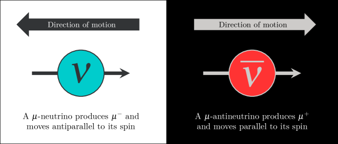
Figure 1.1: The chiral (or V–A) nature of the charged-current interactions allows us to define what is a neutrino and what is an antineutrino in the ultrarelativistic limit, when chirality coincides with helicity and the value of the mass plays only a minor role.

In the Fermi theory (or generally in quantum field theory) the leptonic charged current describes the transition from one neutral lepton to a charged one and the other reactions connected by the crossing symmetry. The V–A structure of weak interactions means that this current has the form,

$$V_{\mu}^{\mathrm{lept}}-A_{\mu}^{\mathrm{lept}}=\bar{e}\gamma_{\mu}\nu-\bar{e}\gamma_{\mu}\gamma_{5}\nu=2\bar{e}\gamma_{\mu}P_{\mathrm{L}}\nu$$ (1.1)

where we introduced the chirality projector $P_{\mathrm{L}}=(1-\gamma_{5})/2$. This structure implies that the wave-functions of the neutrinos and of the antineutrinos appear necessarily in the combinations,

$$\psi_{\nu}(x)=e^{-ipx}P_{\mathrm{L}}\;u\quad\text{and}\quad\psi_{\bar{\nu}}(x)=e^{-ipx}P_{\mathrm{R}}\;u$$ (1.2)

where the 4-spinors $u$ obey the Dirac equation and where we have considered plane waves for definiteness, thus $p\;x=p_{\mu}\,x^{\mu}=Et-\vec{p}\cdot\vec{x}$; of course, the energy is $E=\sqrt{p^{2}+m^{2}}$ where $p=|\vec{p}\,|$ is the momentum and $m$ is the mass. (The wave-functions that appear in eq. (1.2) are proportional to the functions $\psi_{i}$ that appear in the field definition that will be given in (2.10); their properties concerning the chirality projectors can be derived using the results on charge conjugation described in Section A.2.)

In the ultrarelativistic limit $p\gg m$ we have $E\approx p$ and the Dirac hamiltonian that rules the propagation of a massive fermion can be written as,

$$H_{\mathrm{D}}=\vec{\alpha}\cdot\vec{p}+\beta m\approx\vec{\alpha}\cdot\vec{p}=\vec{\Sigma}\cdot\vec{p}\,\gamma_{5}\approx\vec{\Sigma}\cdot\vec{n}\,\gamma_{5}\,E$$ (1.3)

where $\vec{n}=\vec{p}/p$ is the direction of the momentum. The projection of the spin in the direction of the momentum, ${\vec{\Sigma}\cdot\vec{n}}$, is called the helicity. Thus, when the kinetic energy is much larger than the mass, we find that the energy eigenstates given in (1.2) satisfy,

$${\vec{\Sigma}\cdot\vec{n}}\;\psi_{\nu}(x)\approx-\psi_{\nu}(x)\quad\text{and}\quad{\vec{\Sigma}\cdot\vec{n}}\;\psi_{\bar{\nu}}(x)\approx+\psi_{\bar{\nu}}(x)$$ (1.4)

Stated in plain words, we see that, in the ultrarelativistic limit, neutrinos have negative helicity whereas antineutrinos have positive helicity. In other terms, we have another way to identify what is a neutrino and what is an antineutrino, as illustrated in Figure 1.1. However, in this manner the question arises: what happens if the mass is non-zero and we invert the direction of the momentum? Is it possible to retain a distinction between neutrinos and antineutrinos?

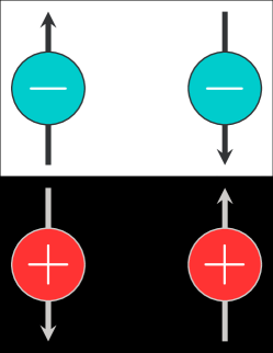
(a) Dirac states.

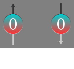
(b) Majorana states.

Figure 1.2: Massive fields in their rest frames. The arrows show the possible directions of the spin. 1.2(a) shows the 4 states of a Dirac massive field. The signs indicate the charge that distinguishes particles and antiparticles, e. g. the electric charge of an electron. 1.2(b) shows the 2 states of a Majorana massive field. The symbol “zero” indicates the absence of any charge (not only of the electric charge): particles and antiparticles coincide.

Neutrino masses

The answers to the questions raised just above are not known and to date we have to rely on theoretical considerations. The main hypotheses that are debated are the following two:

1. The mass of neutrinos has the same character as the mass of any other charged spin 1/2 particles; in more formal terms, we assume the same type of mass originally hypothesized by Dirac for the electron. A closer example is the neutron, that is a neutral particle just as the neutrino. In a relativistic quantum field theory, this type of mass entails a strict separation between particle and antiparticle states. More in details, it means that in the rest frame there are four distinct states, as for the neutron or the electron, namely, 2 spin states for the neutrino and 2 spin states for the antineutrino. This is illustrated in Figure 1.2(a). If we accelerate the 2 neutrino states — depicted in blue in Figure 1.2(a) — at ultrarelativistic velocity and in the direction of the spin, one of these state will be allowed to react with the matter through weak interactions, whereas the other state will not; the same is true for antineutrinos.

2. The second hypothesis is the one put forward by Majorana. In this case, there are just 2 spin states in the rest frame; the symmetry under rotations implies that these are two states of the same particle, or in other words, particle and antiparticle coincide. This is illustrated in Figure 1.2(b). This hypothesis can be reconciled with the property of weak interactions, summarized in Figure 1.1, simply remarking that helicity is not an invariant quantity for a massive particle. Therefore, the distinction between neutrinos and antineutrinos is just a feature of ultrarelativistic motions and not a fundamental one. This hypothesis is more economical than the previous one, being based on a smaller number of states, and it is considered plausible by many theorists, for various reasons that we will not examine here in detail.

Arguably, the question of settling which of these hypotheses is correct is the most important open question in neutrino physics to date. In principle, it would be possible to observe the difference between the two types of masses in some experiments even if we know that the effects we are searching for experimentally are quite small.

The difference between the two type of masses is however irrelevant for the description of other important phenomena, including neutrino oscillations. In fact the main experimental evidence arising from the Majorana mass would be the total lepton number violation. On the contrary, neutrino oscillations concern $\nu_{\ell}\rightarrow\nu_{\ell}^{\prime}$ and $\bar{\nu}_{\ell}\rightarrow\bar{\nu}_{\ell}^{\prime}$ transitions, i.e., a transformation from one lepton to another lepton, and not a violation of the total lepton number. This shows that the distinctive feature of Majorana mass is not probed. This was first remarked and proved in Ref. [10] and will be discussed in the following.

1.1.3 The major role of relativity for neutrinos

From the standpoint of the standard model of elementary particle, all fermions have a similar status. However, electrons and neutrinos behave very differently in many situations. One reason of this difference is just the velocity of the motion. The external electrons of an atom revolve with a slow velocity $v\sim c\times\alpha$, where $\alpha\approx 1/137$ is the fine structure constant: thus, the role of relativistic considerations is not very central. By contrast, relativity is of paramount relevance for neutrinos, for several (more or less evident) reasons that will be recalled here.

Smallness of neutrino mass

Since the beginning it was believed that neutrinos have a small mass (Pauli, Fermi, Perrin). Its existence was demonstrated only recently and, despite the fact we do not know its precise value yet, we are sure that it is more than one million times smaller than the mass of the electron. The main experiment that will investigate neutrino mass in laboratory is the KArlsruhe TRItium Neutrino (KATRIN): it aims to study the endpoint region of the tritium decay hoping to improve by 10 times the current upper limit of $2.0\text{\,}\mathrm{eV}$, combined results of Mainz and Troitsk experiments. In the context of three neutrino oscillations, these results can be compared directly with other ones: those from SN1987A (or those from pion and tau decay) are (much) weaker than those described above, while the most recent combined cosmological analyses claim much tighter limits, that in fact have the potential to discriminate the neutrino mass spectrum. As discussed above, not only the “absolute” value of the neutrino masses, but also the nature of the mass is at present unknown.

Features of the main phenomena of neutrino emission

Neutrinos are emitted in nuclear transitions where a typical kinetic energy ranges from few keV to some MeV; the lowest energy neutrinos observed by Borexino (solar neutrinos) have few hundreds $\mathrm{keV}$. In many high energy processes neutrinos are emitted with much larger kinetic energies: the highest energy events attributed to neutrinos are those seen by IceCube with energy of few $\mathrm{PeV}$. In all practical cases in which we will be interested here, the kinetic energy is much more than the mass, and neutrinos propagate in the ultrarelativistic regime.

Cross sections growth with energy

Neutrino interactions, as a rule, increase with their energy $E_{\nu}$. In fact there is a characteristic constant named after Fermi, $G_{\mathrm{F}}$, that appears in the amplitude of neutrino interactions. This has dimensions of an area (or equivalently an inverse energy squared) thus any cross section behaves typically as $\sigma\sim G_{\mathrm{F}}^{2}E^{2}_{\nu}$ or $G_{\mathrm{F}}^{2}mE_{\nu}$, where $m$ is some characteristic mass. Incidentally, the main feature of neutrinos, namely the smallness of their cross sections of interactions (weak interactions) is evident from the numerical value of,

$$G_{\mathrm{F}}^{2}=$5.297\text{\times}{10}^{-44}\text{\,}{\mathrm{cm}}^{2}\text{\,}{\mathrm{MeV}}^{-2}$$$ (1.5)

This is why these particles have been observed only at relatively high energies. Moreover, as discussed above in most cases (and all cases of interest for the study of oscillations) we can assume that neutrinos are produced in ultrarelativistic conditions.

Helicity (spin-momentum correlation)

In weak interactions ultrarelativistic neutrinos (resp., antineutrinos) have as a rule the spin antialigned (resp., aligned) with the momentum. This is completely different from what happens to the electrons in atomic physics, where the spin can be both up or down. Various aspects of this connection have been discussed in Section 1.1.2, stressing the assumption $p\gg m$. We add here only one formal remark. When we consider ultrarelativistic motions the wave equations for neutrinos and antineutrinos can be written as a pair of Weyl equations, namely,

$$i\;\partial_{t}\;\phi=\mp\,\vec{\sigma}\cdot\vec{p}\;\phi$$ (1.6)

where $\sigma_{i}$ are the Pauli matrices and $\vec{p}=-i\vec{\nabla}$. In this formalism, the role of helicity is very transparent. (Formally, this remark concerns the structure of the Dirac equation and becomes evident in the representation of the Dirac matrices in which the chirality matrix $\gamma_{5}$ is diagonal: see Section A.1 and A.3.)

Role of antineutrinos

Finally, unlike atomic physics where the existence of positrons and anti-baryons can be neglected, in most practical applications neutrinos and antineutrinos have the same importance: consider, for instance, big bang or supernovae events that have energies at which the particle-antiparticle production cannot be neglected. Note that the possibility to create (or to destroy) particles is a specific feature of relativistic phenomena. Indeed, the model of Fermi was proposed since the start as a relativistic quantum field theory.

To summarize, we have described the main reasons why neutrinos are, as a rule, ultrarelativistic and the theory of neutrinos has to be a relativistic theory. This implies that the formalism to describe neutrinos differs to large extent from the one commonly used for the physics of the electrons in the atoms, i.e., of ordinary matter.

Section 1.2 Introduction to oscillations

As mentioned above, three different types of neutrinos (called also flavor) exist. It is common usage to call neutrino oscillations the observable transformation of a neutrino from one type to another, from the moment when it was produced to the moment when it is detected. In his Nobel lecture (1995), Reines depicts this phenomenon by using the vivid allegory of the “dog which turns into a cat” which, however, causes a rather disconcerting feeling, being quite far from what we experience in reality.

As remarked immediately by its discoverers, neutrino oscillation is a typical quantum mechanics phenomenon, that can be easily described resting on the wave nature of neutrinos. In order to introduce it as effectively as possible, we consider 3 different physical systems in the following. The first is just the propagation of polarized light in a birefringent crystal, the second is the spin states of an electron in a magnetic field, the third one is the neutral kaon system. All these systems can be considered as sources of precious analogies for us; the last one was originally invoked to introduce neutrino oscillations (Pontecorvo, 1957).

Transformation of the polarization states of the light

Consider a wave guide (or a transparent crystal) on a table, oriented along the (horizontal) $x$-axis and assume that the two orthogonal directions $y$ and $z$ have different refractive indices $n_{y}$ and $n_{z}$; e.g., a birefringent crystal. Suppose that a plane wave that propagates along the $x$-axis enters the crystal and that it is linearly polarized at $45^{\circ}$ in the $y-z$ plane, bisecting the 1st-3rd quadrants. This polarization is realized when the two oscillating components of the electric field on the $y$ and $z$ axes have a phase difference $\delta=0$. Inside the crystal, the first component propagates according to,

$$\exp\!\left[{2\pi i\left(\frac{x}{\lambda_{y}}-\frac{t}{T}\right)}\right]\quad\text{with}\quad\lambda_{y}=\frac{\lambda_{0}}{n_{y}}$$ (1.7)

and similarly for the $z$-component. Owing to the fact that the two refractive indices are different, the relative phase between the $y$ and the $z$ components changes. In particular, if the length of the crystal $L$ satisfies the condition,

$$\delta(L)=2\pi(n_{y}-n_{z})\frac{L}{\lambda_{0}}=\pi$$ (1.8)

the wave will exit with a polarization at $135^{\circ}$, that bisects the 2nd-4th quadrants. Thus, the wave will be orthogonal to the initial wave, the one that entered the crystal. (This device and arrangement is called in optics waveplate.)

Another description of the same phenomenon is as follows. The definition $n={\lambda_{0}}/{\lambda}$ used above implies,

$$n=\frac{c}{v_{\mathup{{{p}}}}}$$ (1.9)

where $v_{\mathrm{p}}=\lambda/T=\omega/k$ is the phase velocity; thus, the phase velocities are different in the $y$ and $z$ directions. We can then say that the components of the wave in the $y$ and $z$ directions propagate with different velocities and this causes the relative change of phase, that modifies the polarization of the propagating wave (and/or of the photons).

An important remark concerns the interpretation of this situation in terms of photons, i.e. the impinging photons get transformed into their orthogonal states. This conclusion is quite dramatic indeed and we are entitled to talk of transmutation or transformation of photons.

Transformation of the spin states of an electron

Consider a region where there is a magnetic field aligned along the $z$ axis with intensity $B$ and an electron whose spin lies in the $x-y$ plane. It is evident to any physicist that, in this situation, the spin of the electron will remain in the plane and simply revolve, in a motion of precession around the $z$ axis.

Let us examine this situation from the point of view of quantum mechanics. The (matrix elements of the spin) wave-function that describes an electron, polarized in the $x$ direction at time $t=0$, is,

$$\psi_{x+}(0)=\frac{1}{\sqrt{2}}\left(\begin{array}[]{c}1\\ 1\end{array}\right)$$ (1.10)

The (matrix elements of the spin) hamiltonian, that describes the coupling of $\vec{B}$ to the magnetic moment $\vec{\mu}$, is,

$$H=-\vec{B}\cdot\vec{\mu}=\left(\begin{array}[]{cc}-B\mu&0\\ 0&B\mu\end{array}\right)$$ (1.11)

The state of the electron will be not stationary and it is easy to find the solution of the Schrödinger equation as,

$$\psi_{x+}(t)=\frac{1}{\sqrt{2}}\left(\begin{array}[]{c}e^{i\Phi}\\ e^{-i\Phi}\end{array}\right)\quad\text{where}\quad\Phi=\frac{B\ \mu\ t}{\hbar}$$ (1.12)

This implies for instance that the electron will not remain polarized in the direction of the $x$-axis in the course of the time and in fact, it can eventually turn into an orthogonal state. In order to verify this statement, we evaluate the probability to find it in the state with opposite polarization, namely aligned along,

$$\psi_{x-}(0)=\frac{1}{\sqrt{2}}\left(\begin{array}[]{c}1\\ -1\end{array}\right)$$ (1.13)

It is straightforward to verify that,

$$P_{x+\to x-}(t)\equiv\left|\>\langle\psi_{x-}(0)|\psi_{x+}(t)\rangle\>\right|^{2}=\left|\frac{e^{i\Phi}-e^{-i\Phi}}{2}\right|^{2}=\sin^{2}\!\left[\frac{B\ \mu\ t}{\hbar}\right]$$ (1.14)

which is non-zero, it is between $0$ and $1$ as any respectable probability, it has an oscillatory character and in fact it becomes 1 (signaling a full transformation) when $\Phi=\pi/2$.

Transformation of neutral kaons

Shortly after the discovery of $K$-mesons (kaons) and $\Lambda$-particles, it was realized that a new quantum number, strangeness, is conserved by strong interactions. The neutral kaon $\mathup{{{K}}^{\scriptstyle{0}}}$ produced e.g., in $\mathup{{{\pi}}^{\scriptstyle{-}}}+\mathup{{{p}}}\to\mathup{{{K}}^{\scriptstyle{0}}}+\Lambda$, having an internal non-vanishing strangeness quantum number, is different from its own antiparticle $\mathup{{\overline{{K}}}^{\scriptstyle{0}}}$. Gell-Mann and Pais in 1955 remarked that the common decay channel $\mathup{{{K}}^{\scriptstyle{0}}}$ or $\mathup{{\overline{{K}}}^{\scriptstyle{0}}}\to\mathup{{{\pi}}^{\scriptstyle{+}}}\mathup{{{\pi}}^{\scriptstyle{-}}}$ implies necessarily the existence of non-zero transition amplitudes $\langle\mathup{{{\pi}}^{\scriptstyle{+}}}\mathup{{{\pi}}^{\scriptstyle{-}}}|H_{\mathrm{weak}}|\mathup{{{K}}^{\scriptstyle{0}}}\rangle$ and $\langle\mathup{{{\pi}}^{\scriptstyle{+}}}\mathup{{{\pi}}^{\scriptstyle{-}}}|H_{\mathrm{weak}}|\mathup{{\overline{{K}}}^{\scriptstyle{0}}}\rangle$ at the order $G_{\mathrm{F}}$. Thus, strangeness is not respected in weak interactions. The effective hamiltonian of the two neutral kaons has non-zero transition element $\langle\mathup{{{K}}^{\scriptstyle{0}}}|H_{\mathrm{eff}}|\mathup{{\overline{{K}}}^{\scriptstyle{0}}}\rangle=\delta m-i\>{\delta\Gamma}/{2}$, namely,

$$H_{\mathrm{eff}}=\left(\begin{array}[]{cc}M&\delta m\\ \delta m^{*}&M\end{array}\right)-\frac{i}{2}\left(\begin{array}[]{cc}\Gamma&\delta\Gamma\\ \delta\Gamma^{*}&\Gamma\end{array}\right)$$ (1.15)

where,

$$M=\mathcal{O}(1)\quad\text{and}\quad\Gamma,\delta m,\delta\Gamma=\mathcal{O}(G_{\mathrm{F}}^{2})$$ (1.16)

with the non-hermitian part accounting for the weak decays. This hamiltonian is non-diagonal, thus the propagation eigenstates differ from the strangeness eigenstates $\mathup{{{K}}^{\scriptstyle{0}}}$ and $\mathup{{\overline{{K}}}^{\scriptstyle{0}}}$. These are indicated with $\mathup{{{K}}{}_{\scriptstyle{L}}^{\scriptstyle{0}}}$ and $\mathup{{{K}}{}_{\scriptstyle{S}}^{\scriptstyle{0}}}$, from “long” and “short” (with reference to their very different lifetimes) and are occasionally called also weak eigenstates. Even if their mass difference is so small that it cannot be measured directly, it entails the occurrence of “virtual transitions $\mathup{{{K}}^{\scriptstyle{0}}}\leftrightarrows\mathup{{\overline{{K}}}^{\scriptstyle{0}}}$”, quoting the words of Gell-Mann and Pais. More in detail, a $\mathup{{{K}}^{\scriptstyle{0}}}$ produced at the time $t=0$ is a combination of $\mathup{{{K}}{}_{\scriptstyle{L}}^{\scriptstyle{0}}}$ and $\mathup{{{K}}{}_{\scriptstyle{S}}^{\scriptstyle{0}}}$, so it is possible that it will be detected as a $\mathup{{\overline{{K}}}^{\scriptstyle{0}}}$ at a subsequent time $t$. This phenomenon is called kaon transformations or transmutation or (with the modern language) kaon oscillations.

Another interesting behavior of the neutral kaon system was predicted in 1955 by Pais and Piccioni: since $\mathup{{{K}}^{\scriptstyle{0}}}$ and $\mathup{{\overline{{K}}}^{\scriptstyle{0}}}$ interact differently with nuclei, the eigenstates of propagation in the ordinary matter are not $\mathup{{{K}}{}_{\scriptstyle{L}}^{\scriptstyle{0}}}$ and $\mathup{{{K}}{}_{\scriptstyle{S}}^{\scriptstyle{0}}}$. Thus, when a beam of $\mathup{{{K}}{}_{\scriptstyle{L}}^{\scriptstyle{0}}}$ traverses a slab of matter, we will have also $\mathup{{{K}}{}_{\scriptstyle{S}}^{\scriptstyle{0}}}$ at the exit. This phenomenon is called kaon regeneration.

The inception of neutrino oscillations

After the experimental observation of the kaon transformation phenomenon, Pontecorvo (1957) asked whether something similar could occur to other systems such as neutrino-antineutrino, neutron-antineutron, atoms-antiatoms. While this does not correspond to the current physical picture of the phenomenon, it is its first specific description in the scientific literature. Later, Maki, Nakagawa and Sakata (1962) mentioned the possible occurrence of virtual transmutation of neutrinos, again without elaborating the details. This was emended, once again, by Pontecorvo who described the modern formalism in 1967. It was the phenomenon of kaons regeneration that inspired Emilio Zavattini to ask Lincoln Wolfenstein about the possible occurrence of something similar in neutrino physics. (Note the interesting fact, the former was an experimentalists and the latter a theorist, just as in the case of Stas Mikheyev and Alexei Smirnov. Similarly, Pontecorvo belonged to a school of physicists where the distinction between theorists and experimentalists was quite vague.)

Chapter 2 Leptonic mixing

Section 2.1 General considerations

2.1.1 Definition and context

Neutrino flavor states

The concept of neutrino with given flavor identifies the neutral particle associated by weak interactions to the charged leptons with given flavor, namely the electron, the muon or the tau. For what we know to date, the association works in such a manner that the flavor is conserved in the interaction point. This allows us to define, e.g., a $\mathup{{{\nu}}{}_{\scriptstyle{\!e}}}$ as the particle associated to the $\mathup{{{e}}^{\scriptstyle{+}}}$ in the $\beta^{+}$ decay of ³⁰P, or equivalently, the state emitted in electron capture processes, say, $\mathup{{{e}}^{\scriptstyle{-}}}+\text{\textsuperscript{37}Ar}\to\mathup{{{\nu}}{}_{\scriptstyle{\!e}}}+\text{\textsuperscript{37}Cl}$. A similar definition holds true for antineutrinos.

At the basis of this definition is the assumption, consistent with all known facts, that charged-current weak-interactions are described by a relativistic quantum field theory, that is Fermi theory at low energies and the standard electroweak model — based on $\mathrm{SU}(3)_{\mathrm{C}}\times\mathrm{SU}(2)_{\mathrm{L}}\times\mathrm{U}(1)_{\mathrm{Y}}$ — at higher ones. For this reason, many different processes involve to the same type of neutrino, just as in the previous example with $\mathup{{{\nu}}{}_{\scriptstyle{\!e}}}$. Another hidden assumption is that neutrino masses play a negligible role in these interactions, as we will discuss here.

Neutrino mixing

Let us assume that the quantized neutrino fields that have given flavor $\nu_{\ell}$ do not coincide with quantized neutrino fields that have given mass but rather they coincide with linear combinations of fields $\nu_{i}$ that have given mass $m_{i}$, namely,

$$\nu_{\ell}=\sum_{i=1}^{N}U_{\ell i}\ \nu_{i}\quad\text{with}\quad\begin{cases}\ell=\mathrm{e},\mu,\tau&\text{[flavor]}\\ i=1,2,3&\text{[mass]}\end{cases}$$ (2.1)

where $U_{\ell i}$ are the elements of the leptonic mixing matrix. In the following, we will emphasize the case of three light neutrinos, $N=3$, and we will assume that $U_{\ell i}$ are the elements of a $3\times 3$ unitary matrix. These assumptions are consistent: 1. with the measured width of $\mathup{{{Z}}^{\scriptstyle{0}}}$, that receives a contribution from the 3 light neutrinos; 2. with the fact that the neutrinos with given flavors have all the same interactions — they are universal; 3. with cosmological observations. The existence of a sizable admixture with other neutrinos would imply new phenomena (if they are heavy, it would result into non-unitarity of the $3\times 3$ part of the mixing matrix and it could lead to observable violations of flavor universality) that currently are not observed.

Connection with Lagrangian densities

The above situation holds true, for instance, if we assume that the mass of neutrinos are described by a Dirac Lagrangian density,

$$\mathcal{L}_{\mathrm{D}}=-\sum_{\ell,\ell^{\prime}}\left(\overline{\nu_{\ell\mathrm{R}}}\mathcal{M}_{\ell\ell^{\prime}}^{\mathrm{D}}\nu_{\ell^{\prime}\mathrm{L}}+\overline{\nu_{\ell^{\prime}\mathrm{L}}}(\mathcal{M}_{\ell\ell^{\prime}}^{\mathrm{D}})^{\dagger}\nu_{\ell\mathrm{R}}\right)$$ (2.2)

with,

$$\mathcal{M}^{\mathrm{D}}=V\;\mathrm{diag}(m_{1},m_{2},m_{3})\,U^{\dagger}$$ (2.3)

where $\nu_{\ell^{\prime}\mathrm{L}}=P_{\mathrm{L}}\nu_{\ell^{\prime}}$ and $\nu_{\ell\mathrm{R}}=P_{\mathrm{R}}\nu_{\ell}$ are the projections of the neutrino field — later expanded in oscillators, see (2.10) and (2.15) — in the left handed and right handed subspaces, with $P_{\mathrm{R,L}}=(1\pm\gamma_{5})/2$, and $V$ is another mixing matrix, that concerns only right neutrino fields; it can be set equal to $U$ when we are interested only in neutrino oscillations and if we assume that only the known forces are present. The same mixing matrix $U$ stems from a Majorana Lagrangian density,

$$\mathcal{L}_{\mathrm{M}}=-\frac{1}{2}\sum_{\ell,\ell^{\prime}}\left(\overline{\nu_{\ell\mathrm{R}}^{\mathrm{c}}}\mathcal{M}_{\ell\ell^{\prime}}^{\mathrm{M}}\nu_{\ell^{\prime}\mathrm{L}}+\overline{\nu_{\ell^{\prime}\mathrm{L}}}(\mathcal{M}_{\ell\ell^{\prime}}^{\mathrm{M}})^{\dagger}\nu_{\ell\mathrm{R}}^{\mathrm{c}}\right)$$ (2.4)

with,

$$\mathcal{M}^{\mathrm{M}}=U^{*}\mathrm{diag}(m_{1},m_{2},m_{3})U^{\dagger}$$ (2.5)

where we can define one right-spinor in terms of the left-spinor by using the charge conjugation matrix as follows, $\nu^{\mathrm{c}}_{\mathrm{R}}\equiv C\overline{\nu_{\mathrm{L}}}^{\mathrm{t}}$. From this definition, we derive $\overline{\nu_{R}^{\mathrm{c}}}=-\nu^{\mathrm{t}}_{\mathrm{L}}C^{-1}$; see Section A.2 for further discussion on the charge conjugation matrix and on its properties. Let us clarify that the fields $\nu_{\ell}$ with $\ell=\mathrm{e},\mu,\tau$ that we consider in the rest of our discussion are the left chiral fields implied by ordinary weak interactions and the presence of the chiral projector $P_{\mathrm{L}}$ is not indicated but only to simplify the notations.

2.1.2 Relation between flavor and mass states

Plane waves

Let us assume that the free neutrinos are confined in a cube of volume $V=L^{3}$ subject to periodicity conditions, so that the momenta are ‘quantized’, i.e., are given in terms of integer numbers $n_{x},n_{y},n_{z}$ as $p_{x}=n_{x}\times 2\pi/L$, $p_{y}=n_{y}\times 2\pi/L$, $p_{z}=n_{z}\times 2\pi/L$. We identify the states fully by means of helicity, and use bi-spinors with given helicity, namely, $(\vec{\sigma}\cdot\vec{p}/p)\varphi_{\lambda}=\lambda\varphi_{\lambda}$, where $\lambda=\pm 1$. We group the momentum and the helicity in the collective label,

$$\alpha=\vec{p},\lambda$$ (2.6)

to shorten a bit the notation.

In the “standard” representation of the Dirac matrices the plane waves of free neutrinos of mass $m_{i}$ are the eigenvectors of the Dirac hamiltonian $H_{\mathrm{D}}$ given by,

$$\psi_{i}(\vec{x},\alpha)=\frac{\exp(i\,\vec{p}\,\vec{x})}{\sqrt{2V}}\left(\begin{array}[]{c}\sqrt{1+\varepsilon_{i}}\ \varphi_{\lambda}\\ \lambda\sqrt{1-\varepsilon_{i}}\ \varphi_{\lambda}\\ \end{array}\right)\quad\text{where}\quad\epsilon_{i}=\frac{m_{i}}{E_{i}}$$ (2.7)

namely $H_{\mathrm{D}}\psi_{i}=E_{i}\psi_{i}$ with $E_{i}=\sqrt{p^{2}+m_{i}^{2}}$. We recall incidentally that the bi-spinors are usually grouped into four-spinors,

$$u_{i}(\alpha)=\frac{1}{\sqrt{2}}\left(\begin{array}[]{c}\sqrt{1+\varepsilon_{i}}\ \varphi_{\lambda}\\ \lambda\sqrt{1-\varepsilon_{i}}\ \varphi_{\lambda}\\ \end{array}\right)$$ (2.8)

that are normalized according to, $u^{\dagger}u=1$. We use this notation occasionally, see e.g., (3.43). The single-particle (non-relativistic) normalization conditions hold true: $\int\mathrm{d}^{3}x\;\psi^{\dagger}\psi=1$ for the plane waves and $\varphi^{\dagger}_{\lambda}\varphi_{\lambda}=1$ for the bi-dimensional spinors.

In the typical situation when the neutrinos are ultrarelativistic, these functions take a mass independent universal form,

$$\psi_{i}(\vec{x},\alpha)\approx\psi(\vec{x},\alpha)\quad\text{with}\quad\psi(\vec{x},\alpha)=\frac{\exp(i\,\vec{p}\,\vec{x})}{\sqrt{2V}}\left(\begin{array}[]{c}\varphi_{\lambda}\\ \lambda\;\varphi_{\lambda}\\ \end{array}\right)$$ (2.9)

The reason why we do not show the dependence of the time is that, immediately below, we introduce quantized fields, given in the interaction representation.

Fields and oscillators

We begin from the quantized field of a neutrino with mass $m_{i}$,

$$\nu_{i}(x)=\sum_{\alpha}\left(a_{i}(t,\alpha)\,\psi_{i}(\vec{x},\alpha)+b_{i}^{\dagger}(t,\alpha)\,\psi_{i}^{\mathrm{c}}(\vec{x},\alpha)\right)$$ (2.10)

where,

$$\begin{cases}a_{i}(t,\alpha)=a_{i}(\alpha)e^{-iE_{i}t}\\ b_{i}(t,\alpha)=b_{i}(\alpha)e^{-iE_{i}t}\end{cases}$$ (2.11)

Once again, the index $i$ corresponds to the mass of the neutrino. Above, we introduced the charge conjugate spinor,

$$\psi_{i}^{\mathrm{c}}=C\overline{\psi_{i}}^{\mathrm{t}}$$ (2.12)

see Section A.2 for a reminder. The oscillators $a_{i}$ and $b_{i}$ are dimensionless operators that obey the condition

$$\{a^{\dagger}(\alpha),a(\beta)\}=\delta_{\alpha\beta}$$ (2.13)

namely there is one independent fermionic oscillator each value of $\alpha$. The above field describes a Dirac neutrino or also a Majorana neutrino, simply replacing $b_{i}=a_{i}.$

We are interested in the neutrino field,

$$\nu_{\ell}(x)=U_{\ell i}\ \nu_{i}(x)$$ (2.14)

where the repeated index $i$ is summed over. If we consider ultrarelativistic neutrinos $p\gg m_{i}$, and if we do not measure the energy too precisely (so to identify the various mass components), we see from (2.9) that the field with given flavor, that is associated to the corresponding charged lepton, can be approximated to,

$$\nu_{\ell}(x)\approx\sum_{\alpha}\left(a_{\ell}(t,\alpha)\,\psi(\vec{x},\alpha)+b_{\ell}^{\dagger}(t,\alpha)\,\psi^{\mathrm{c}}(\vec{x},\alpha)\right)$$ (2.15)

with the very important identification,

$$\begin{cases}a_{\ell}(t,\alpha)=U_{\ell i}\ a_{i}(t,\alpha)\\ b_{\ell}(t,\alpha)=U_{\ell i}^{*}\ b_{i}(t,\alpha)\end{cases}$$ (2.16)

It is crucial to note that, in this approximate expression:

• the plane waves have the same ‘universal form’ $\psi$ valid in the ultrarelativistic limit;

• the operators with given flavor $\ell$, namely $a_{\ell}$ and $b_{\ell}$, are weighted sums of operators with given mass;

• the particle ($a_{\ell}$-type) operators are summed with the matrix $U_{\ell i}$ whereas the antiparticle ($b_{\ell}$-type) operators with its conjugate $U_{\ell i}^{*}$.

Momentum eigenstates

We can simplify the formulae even further when we consider the fact that the neutrino fields are always multiplied by the left chiral projector $P_{\mathrm{L}}=(1-\gamma_{5})/2$ in the known weak interactions. For this reason, as it is well known, we will have only neutrinos with negative helicity $\lambda=-1$ and antineutrinos with positive helicity $\lambda=+1$ in the ultrarelativistic (UR) limit. Therefore, we can write,

$$\begin{cases}a_{\ell}(t,\vec{p},-)=U_{\ell i}\ a_{i}(\vec{p},-)\ e^{-iE_{i}t}&\text{for UR neutrinos}\\ b_{\ell}(t,\vec{p},+)=U_{\ell i}^{*}\ b_{i}(\vec{p},+)\ e^{-iE_{i}t}&\text{for UR antineutrinos}\end{cases}$$ (2.17)

In this manner, it is possible to define formally the states of ultrarelativistic neutrino and antineutrinos as,

$$\begin{cases}|\nu_{\ell},\vec{p}\;\rangle\equiv a_{\ell}^{\dagger}(0,\vec{p},-)|0\rangle=U_{\ell i}^{*}|\nu_{i},\vec{p}\;\rangle&\text{for UR neutrinos}\\ |\bar{\nu}_{\ell},\vec{p}\;\rangle\equiv b_{\ell}^{\dagger}(0,\vec{p},+)|0\rangle=U_{\ell i}|\nu_{i},\vec{p}\;\rangle&\text{for UR antineutrinos}\end{cases}$$ (2.18)

and also the evolved vectors in the representation of Schrödinger,

$$\begin{cases}|\nu_{\ell},\vec{p},t\rangle\equiv a_{\ell}^{\dagger}(t,\vec{p},-)|0\rangle=U_{\ell i}^{*}|\nu_{i},\vec{p}\;\rangle e^{-iE_{i}t}&\text{for UR neutrinos}\\ |\bar{\nu}_{\ell},\vec{p},t\rangle\equiv b_{\ell}^{\dagger}(t,\vec{p},+)|0\rangle=U_{\ell i}|\nu_{i},\vec{p}\;\rangle e^{-iE_{i}t}&\text{for UR antineutrinos}\end{cases}$$ (2.19)

A few remarks are in order:

• The mixing matrix enters differently in the relation for neutrinos and antineutrinos states (unless this matrix is real).

• It should be noted that the previous very important equations, derive directly from quantum field theoretical relations.

• Note that we have omitted the helicity labels in the states, or more precisely, we have replaced them with an explicit indication of the character of the state, either neutrino or antineutrino, which is well defined in the ultrarelativistic limit.

Again on the ultrarelativistic limit

In order to complete the discussion in Section 1.1.3 making it more specific, we collect here some final remarks on the ultrarelativistic approximation.

• Consider the lowest energy neutrinos that can be detected to date, namely the solar neutrinos above $\sim$300\text{\,}\mathrm{keV}$$ that can be seen in Borexino, along with the (very conservative) bound of 2 eV on neutrino masses. In this case, the value of the parameter that quantifies the deviation from the UR limit (2.7) is $\epsilon_{i}<10^{-5}$.

• It is possible to think to various situations when the above assumptions do not apply. For example, very near the endpoint of the $\beta$ spectrum, only the lightest neutrino mass state $\nu_{1}$ is emitted together with the electron, and not all three of them, simply to conserve energy. However it is not easy to imagine how to form a usable neutrino beam with this composition.

• More interestingly, the neutrinos produced in the big-bang have now momenta $p\sim kT\approx$0.2\text{\,}\mathrm{meV}$$; the two heavier states have masses larger than $\sqrt{|\Delta m^{2}_{31}|}\approx$50\text{\,}\mathrm{meV}$$ and $\sqrt{\Delta m^{2}_{21}}\approx$8.6\text{\,}\mathrm{meV}$$ and are now non-relativistic. However, a discussion of oscillations is hardly needed, as we can simply treat these states as mass states.

Therefore, for all practical applications, we are interested to discuss neutrino oscillations of the ordinary neutrinos only when the ultrarelativistic limit applies.

Section 2.2 The parameters relevant to oscillations

2.2.1 General considerations

Number of parameters in a unitary matrix

The number of free parameters of a $n\times n$ mixing matrix $U$ satisfying unitarity $UU^{\dagger}=U^{\dagger}U=\mathbb{1}$ is easily found taking into account that there are $n$ constraints $\sum_{i=1}^{n}|U_{\ell i}^{2}|=1$ and two times $n(n-1)/2$ further constraints $\sum_{i=1}^{n}U_{\ell i}^{*}U_{\ell^{\prime}i}=0$, with $\ell\neq\ell^{\prime}$. Thus we have $n^{2}$ real constraints and $n^{2}$ real parameters in the matrix $U$. The determinant is a phase factor that can be explicitly factored out, corresponding to the factorization of the group $\mathrm{U}(n)=\mathrm{U}(1)\otimes\mathrm{SU}(n)$. The same counting can be done even more simply, by considering that a unitary matrix can be written as $U=\exp(iH)$ where $H$ is hermitian; the subgroup $\mathrm{SU}(n)$ corresponds to the subset of the traceless hermitian matrices. Summarizing, in the $2\times 2$ case we have 4 parameters and in the $3\times 3$ case we have 9 of them.

Overall phases do not matter

As we have mentioned just above, the states with given flavor are superpositions of states with given mass and the former evolve in time in a non-trivial manner, acquiring different phase factors. For this reason, flavor transformation occur: this is the conceptual core of the neutrino oscillation phenomena.

Note that in quantum mechanics there is the freedom to define at our will which are the overall phase factors of the states, and in particular, which are the phase factors of the states with given flavor and those with given mass. To be sure, we note that when these phases are changed, the mixing matrix does change. In fact, if we change the phases of the flavor and of the mass states, according to,

$$|\nu_{\ell}\rangle^{\prime}=e^{i\zeta_{\ell}}|\nu_{\ell}\rangle\quad\text{and}\quad|\nu_{i}\rangle^{\prime}=e^{i\zeta_{i}}|\nu_{i}\rangle$$ (2.20)

we will have,

$$|\nu_{\ell}\rangle^{\prime}=(U_{\ell i}^{\prime})^{*}|\nu_{i}\rangle^{\prime}$$ (2.21)

with a mixing matrix where we have changed the phases in all rows and columns,

$$U_{\ell i}^{\prime}=e^{-i\zeta_{\ell}}\ U_{\ell i}\ e^{i\zeta_{i}}$$ (2.22)

On the other hand, it is evident that this redefinition will not change the absolute values,

$$|U_{\ell i}^{\prime}|=|U_{\ell i}|$$ (2.23)

and, most importantly, it will not change the probabilities of transition in which we are interested, such as,

$$|\langle\nu_{\ell_{2}}|\nu_{\ell_{1}},t\rangle|^{2}=|\text{\reflectbox{${}^{\prime}$}}{\langle\nu_{\ell_{2}}}{|\nu_{\ell_{1}},t\rangle^{\prime}}|^{2}$$ (2.24)

where $\text{\reflectbox{${}^{\prime}$}}\langle\nu|$ is the bra corresponding to the ket $|\nu\rangle^{\prime}$; recall that we have $|\nu_{\ell}\rangle\equiv|\nu_{\ell},t=0\rangle$. The possibility to redefine the overall phase factors has however a prominent consequence: not all the $n^{2}$ parameters of a unitary matrix are relevant for the phenomenon that we are interested to discuss. Next, we proceed to count the parameters that, instead, do matter.

Number of parameters relevant to oscillations

The parameters that are relevant to neutrino and antineutrino oscillations are those that are invariant under a redefinition of the phases of the flavor fields and of the mass neutrino fields. Evidently these are less than $n^{2}$, the parameters of a unitary matrix. We present three different ways to count them, in view of the importance of this counting.

1. The standard way to count these parameters is to consider that for each flavor or mass field, we can impose a constraint on $U_{\ell i}$ exploiting the redefinition of the phases of the fields. For instance we can choose to make real a full row and a full column of the mixing matrix; but the two have one parameter in common, thus we can arrange $2n-1$ constraints only.

2. Another consideration that leads to the same conclusion is that we have $n$ phase factors for the flavor fields and $n$ of them for the mass fields, but the global phase factors of the flavor fields and of the mass fields amount to a single effective parameter, not to two.

3. As already noted in (2.23), using different phases of the fields the modulus of the elements of the mixing matrix stays unchanged. Thus, let us count the number of independent parameters $|U_{\ell i}^{2}|$. The unitarity relations $\sum_{i=1}^{n}|U_{\ell i}^{2}|=1$ fix one parameter for each row and similarly for each column. This consideration implies that the real matrix with elements $|U_{\ell i}^{2}|$ has only $(n-1)^{2}$ independent parameters. For example, in the $3\times 3$ example, we have four of them,

   $$\left(\begin{array}[]{lll}\mathrm{free}&\mathrm{free}&\mathrm{fixed}\\ \mathrm{free}&\mathrm{free}&\mathrm{fixed}\\ \mathrm{fixed}&\mathrm{fixed}&\mathrm{fixed}\end{array}\right)$$ (2.25)

All in all, the result is that the number of free (or independent) parameters is,

$$\text{Number of free parameters}=n^{2}-(2n-1)=(n-1)^{2}$$ (2.26)

This means 4 in the $3\times 3$ case while in the $2\times 2$ case we have only 1 relevant parameter.

Angles and phases in the mixing matrix

It is not difficult to identify these free parameters more precisely. First, consider the subclass of unitary matrices that are also real, $U=U^{*}$. It is easy to verify that this corresponds to the orthogonal real matrices, that have $n(n-1)/2$ parameters. These parameters are angles; e.g., in the $2\times 2$ case we are dealing with a single angle, whereas in the $3\times 3$ case we have the three Euler angles. The remaining physical parameters are phases relevant to oscillations,

$$\mbox{Number of phases}=(n-1)^{2}-n(n-1)/2=(n-1)(n-2)/2\quad\text{for}\quad n\geq 2$$ (2.27)

In other words, a $2\times 2$ matrix can be made real by a suitable choice of phase factors, so that no phases have relevance to oscillations, whereas a $3\times 3$ matrix has one physical phase factor relevant to neutrino oscillations.

Quartets

As we will see later, a complex combination of mixing elements, sometimes called quartet, enters the explicit expressions of the oscillation probabilities,

$$\mathcal{Q}_{\ell\ell^{\prime},ij}=U_{\ell i}\;U_{\ell^{\prime}i}^{*}\;U_{\ell j}^{*}\;U_{\ell^{\prime}j}$$ (2.28)

and indeed it has the same value for any choice of the phases of the $\nu_{\ell}$ and $\nu_{i}$ fields — i.e., it is not convention-dependent. Moreover, it satisfies various interesting properties, such as,

$$\begin{cases}\mathcal{Q}_{\ell\ell^{\prime},ij}=\mathcal{Q}_{\ell^{\prime}\ell,ij}^{*}=\mathcal{Q}_{\ell\ell^{\prime},ji}^{*}\;\\ \sum_{i}\mathcal{Q}_{\ell\ell^{\prime},ij}=\delta_{\ell\ell^{\prime}}|U_{\ell j}^{2}|\;\\ \mathcal{Q}_{\ell\ell,ij}=|U_{\ell i}^{2}U_{\ell j}^{2}|\;\\ \dots\end{cases}$$ (2.29)

We can usefully define the real and imaginary parts,

$$\mathcal{Q}_{\ell\ell^{\prime},ij}=R_{\ell\ell^{\prime},ij}+i\ I_{\ell\ell^{\prime},ij}\quad\text{namely}\quad\begin{cases}R_{\ell\ell^{\prime},ij}=\mathrm{Re}[\mathcal{Q}_{\ell\ell^{\prime},ij}]\\ I_{\ell\ell^{\prime},ij}=\mathrm{Im}[\mathcal{Q}_{\ell\ell^{\prime},ij}]\end{cases}$$ (2.30)

which are of interest since the expression of the oscillation probabilities depend upon these two real quantities, as will be discussed in Section 3.1.1. These quantities can be always expressed in terms of the mixing angles and of the physical phase factor, however they are interesting on their own, being parameterization independent. Therefore, we examine here the real part of the quartets $R$ and their imaginary part $I$. We will show (focussing on the 3 flavor case) that it is possible to calculate both of them in terms of the simplest phase-independent quantities, namely $|U_{\ell i}^{2}|$, up to a sign that remains undetermined.

Expression of $R$ and $I$ in terms of $|U_{\ell i}|$

The symmetry properties are as follows: the real part is even in the exchange of $\ell\leftrightarrow\ell^{\prime}$ and $i\leftrightarrow j$, whereas the imaginary one is odd in both exchanges. Thus, in the case $\ell=\ell^{\prime}$, we have,

$$R_{\ell\ell,ij}=|U_{\ell i}^{2}U_{\ell j}^{2}|\quad\text{and}\quad I_{\ell\ell,ij}=0$$ (2.31)

We are also very interested in the cases when $\ell\neq\ell^{\prime}$ and $i\neq j$. The expressions are as follows,

$$R_{\ell\ell^{\prime},ij} = \frac{1}{2}\left(a_{k}^{2}-a_{i}^{2}-a_{j}^{2}\right)$$ (2.32)

$$|I_{\ell\ell^{\prime},ij}| = 2\sqrt{p(p-a_{k})(p-a_{j})(p-a_{i})}$$ (2.33)

with the following definitions,

$$a_{i}=|U_{\ell i}U_{\ell^{\prime}i}|\,;\quad a_{j}=|U_{\ell j}U_{\ell^{\prime}j}|\,;\quad a_{k}=|U_{\ell k}U_{\ell^{\prime}k}|\,;\quad p=(a_{i}+a_{j}+a_{k})/2$$

where $\ell\neq\ell^{\prime}$ and $i,j$ and $k$ are a permutation of $1,2$ and 3. The first expression is immediately obtained by considering the relation $U_{\ell k}U_{\ell^{\prime}k}^{*}=-U_{\ell i}U_{\ell^{\prime}i}^{*}-U_{\ell j}U_{\ell^{\prime}j}^{*}$, taking its absolute value and then recalling the definition of $R_{\ell\ell^{\prime},ij}$. In order to derive the second expression, one can proceed by following steps:

1. Let us define the following complex numbers, $z_{i}=U_{\ell i}U_{\ell^{\prime}i}^{*}$ with $i=1,2,3$, and let us express them as $z_{i}=a_{i}\exp(i\theta_{i})$, where of course $a_{i}=|z_{i}|$.

2. The orthogonality relation $U_{\ell k}U_{\ell^{\prime}k}^{*}+U_{\ell i}U_{\ell^{\prime}i}^{*}+U_{\ell j}U_{\ell^{\prime}j}^{*}=0$ reads $z_{k}+z_{i}+z_{j}=0$, that can be seen as a triangle in the complex plane.

3. Its area is $A=|a_{i}a_{j}\sin\theta_{ij}/2|$ where we introduced the angle $\theta_{ij}=\theta_{i}-\theta_{j}$ between two sides.

4. If we rewrite $I_{\ell\ell^{\prime},ij}=\mathrm{Im}[z_{i}z_{j}^{*}]=\mathrm{Im}[a_{i}e^{i\theta_{i}}a_{j}e^{-i\theta_{j}}]=a_{i}a_{j}\sin\theta_{ij}=2\times A$, we realize that the absolute value of this quantity is twice the area of the above triangle.

5. But the area can be evaluated also with Heron’s formula, since length of the sides is $|z_{i}|=a_{i}$ with $i=1,2,3$.

It is remarkable that just as we have a single phase, we have a single imaginary quantity in the three neutrino case, e.g.,

$$I_{\mathrm{e}\mu,12}=-I_{\mathrm{e}\tau,12}=+I_{\mathrm{e}\tau,13}=...$$ (2.34)

The proof of the first relation goes as follows: let us consider,

$$I_{\mathrm{e}\mu,12}=\mathrm{Im}\left[U_{\mathrm{e}1}U_{\mu 1}^{*}U_{\mathrm{e}2}^{*}U_{\mu 2}\right]$$ (2.35)

From the orthogonality relation, we have,

$$I_{\mathrm{e}\mu,12}=\mathrm{Im}\left[U_{\mathrm{e}1}U_{\mathrm{e}2}^{*}\left(-U_{\mathrm{e}1}^{*}U_{\mathrm{e}2}-U_{\tau 1}^{*}U_{\tau 2}\right)\right]$$ (2.36)

that is also equal to,

$$-\mathrm{Im}[U_{\mathrm{e}1}U_{\mathrm{e}2}^{*}U_{\tau 1}^{*}U_{\tau 2}]=-I_{\mathrm{e}\tau,12}$$ (2.37)

which is the desired relation. Similarly, we can obtain the other ones. An interesting consequence of this result is that, if some element of the mixing matrix is zero, this quantity will be zero. Conversely, a necessary condition for this quantity to be large is that all the elements of the mixing matrix are large. (More on that in the next pages — see (2.44) and (2.45) — and then in Section 3.2.2.)

2.2.2 The standard parameterization

Explicit expression

The leptonic (PMNS) mixing matrix $U$ is conventionally written in terms of the mixing angles $\theta_{12}$, $\theta_{13}$ and $\theta_{23}$ and of the CP-violating phase $\delta$ that plays a role in neutrino oscillations. The most common convention is,

$$U=\left(\begin{array}[]{ccc}c_{12}c_{13}&s_{12}c_{13}&s_{13}e^{-i\delta}\\ -s_{12}c_{23}-c_{12}s_{13}s_{23}e^{i\delta}&c_{12}c_{23}-s_{12}s_{13}s_{23}e^{i\delta}&c_{13}s_{23}\\ s_{12}s_{23}-c_{12}s_{13}c_{23}e^{i\delta}&-c_{12}s_{23}-s_{12}s_{13}c_{23}e^{i\delta}&c_{13}c_{23}\end{array}\right)$$ (2.38)

where $s_{ij},c_{ij}\equiv\sin\theta_{ij},\cos\theta_{ij}$ and where the angles lie in the first quadrant whereas the phase $\delta$ is generic, $\delta\in[0,2\pi)$. Note the usage of the same phase convention and parameterization of the quark (CKM) mixing matrix even if, of course, the values of the parameters are different. This convention makes evident that the CP phase is unphysical if $\theta_{13}\to 0$. Indeed this limit holds if any mixing angle is zero.

Expression in terms of product of matrices

The same matrix can be written as a product of three Euler rotation and a matrix of phases as follows,

$$U=R_{23}\ \Delta\ R_{13}\ \Delta^{*}\ R_{12}$$ (2.39)

where,

$$R_{23} =\left(\begin{array}[]{ccc}1&0&0\\ 0&c_{23}&s_{23}\\ 0&-s_{23}&c_{23}\end{array}\right)\quad R_{13}=\left(\begin{array}[]{ccc}c_{13}&0&s_{13}\\ 0&1&0\\ -s_{13}&0&c_{13}\end{array}\right)$$ (2.40)

$$R_{12} =\left(\begin{array}[]{ccc}c_{12}&s_{12}&0\\ -s_{12}&c_{12}&0\\ 0&0&1\end{array}\right)\quad\hphantom{R_{13}}\Delta=\left(\begin{array}[]{ccc}1&0&0\\ 0&1&0\\ 0&0&e^{i\delta}\end{array}\right)$$

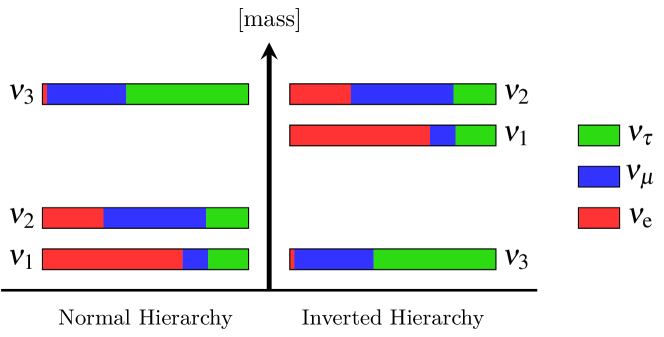
Figure 2.1: Illustration of the mass spectra compatible with the data from neutrino oscillations; left, normal hierarchy; right, inverted hierarchy. The length of the colored bars are proportional to the flavor content of each mass state, $|U_{\ell i}|^{2}$.

An alternative expression

By changing the phases, one can obtain apparently different matrices, whose parameters however maintain the same meaning and therefore describe exactly the same oscillation phenomena. An example of such a choice of some interest is,

$$U^{\prime}=\left(\begin{array}[]{ccc}c_{12}c_{13}&s_{12}c_{13}&s_{13}\\ -c_{12}s_{13}s_{23}-s_{12}c_{23}e^{-i\delta}&-s_{12}s_{13}s_{23}+c_{12}c_{23}e^{-i\delta}&c_{13}s_{23}\\ -c_{12}s_{13}c_{23}+s_{12}s_{23}e^{-i\delta}&-s_{12}s_{13}c_{23}-c_{12}s_{23}e^{-i\delta}&c_{13}c_{23}\end{array}\right)$$

This new choice is somewhat advantageous for the discussion of neutrinoless double beta decay, since the phase $\delta$ does not play any role for the parameter that summarizes the effect of the light Majorana neutrino masses, i.e., $m_{\beta\beta}\equiv\sum_{i}U_{\mathrm{e}i}^{2}m_{i}$. Below, we exhibit a direct construction of the unitary mixing matrix where the single physical phase factor is singled out, that yields the above form of the matrix.

It is quite natural to choose the phases of the fields in order to make real and positive one row and one column. Choosing the ones that cross in $U_{\mathrm{e}3}\equiv\sin\theta\equiv s$ we get,

$$U^{\prime\prime}=\left(\begin{array}[]{ccc|c}&c\;\vec{n}&&s\\ \hline\cr&&&\\ &u&&c\;\vec{m}\\ &&&\\ \end{array}\right)$$ (2.41)

where of course $c=\cos\theta$. Note that in order to have a simpler notation, we assume that the row and column vectors are evident from the context, and do not indicate the transpose sign on the vectors $\vec{m}$ and $\vec{n}$. Here, we introduced two real unit vectors that we can decompose as,

$$\vec{n}=(n_{1},n_{2})=(c_{12},s_{12})\quad\text{and}\quad\vec{m}=(m_{1},m_{2})=(s_{23},c_{23})$$ (2.42)

The $2\times 2$ matrix $u$ is still to be determined. Now, consider the second row $r_{2}$ of the full matrix $U^{\prime\prime}$, with components $r_{2}=(\alpha\;\vec{n}+\beta\;\vec{n}_{\perp}\ ,\ cm_{1})$, where $\alpha$ and $\beta$ are in general two complex numbers and $\vec{n}_{\perp}=(-s_{12},c_{12})$ is a real vector orthogonal to $\vec{n}$. When we impose the orthogonality with the first row, we find that $\alpha=-s\;m_{1}$, and when we impose that $||r_{2}||^{2}=\sum_{i}|U_{\mu i}^{\prime\prime}|^{2}=1$, we find that $|\beta^{2}|=m_{2}^{2}$. Thus we conclude that the second row is $r_{2}=(-sm_{1}\;\vec{n}+e^{i\phi}\ m_{2}\;\vec{n}_{\perp}\ ,\ cm_{1})$. For similar reasons, the third row is $r_{3}=(-sm_{2}\;\vec{n}-e^{i\psi}\ m_{1}\;\vec{n}_{\perp}\ ,\ cm_{2})$. Finally, imposing the orthogonality with the third row, one realizes that $\phi=\psi$. In short, the matrix $u$ defined above is,

$$u=-s\ \vec{m}\otimes\vec{n}+e^{i\phi}\ \vec{m}_{\perp}\otimes\vec{n}_{\perp}$$ (2.43)

Thus, by choosing the parameters $\phi=-\delta$, $\theta=\theta_{13}$ and with the phase choice for $\vec{m}_{\perp}=(c_{23},-s_{23})$, we conclude that $U^{\prime\prime}=U^{\prime}.$

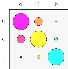
(a) Quark Mixing Elements.

(b) Lepton Mixing Elements.

Figure 2.2: The surfaces of the circles represent the size of the mixing elements, assuming normal mass hierarchy. From top to bottom, from left to right: 2.2(a) quark mixing (CKM) elements $|V_{\mathrm{ud}}|,|V_{\mathrm{us}}|,|V_{\mathrm{ub}}|,|V_{\mathrm{cd}}|,...$; 2.2(b) lepton mixing (PMNS) elements $|U_{\mathrm{e}1}|,|U_{\mathrm{e}2}|,|U_{\mathrm{e}3}|,|U_{\mu 1}|,...$ in both panels, the mixing matrices are supposed to be unitary. The hierarchical structure of quark mixing elements contrasts with the one of lepton mixing elements.

Measure of CP violation

As we have already discussed, for 3 neutrinos there is a single imaginary quantity that signals the presence of a complex mixing matrix, and that, therefore, rules the leptonic CP violation phenomena in neutrino oscillations: see (2.34). In the standard parameterization, the expression of this quantity is,

$$J_{\mathrm{CP}}\equiv I_{\mathrm{e}\mu,12}=s_{13}c_{13}^{2}\;s_{12}c_{12}\;s_{23}c_{23}\;s_{\delta}$$ (2.44)

notice that (consistently with the above discussion) this quantity is bound to vanish if anyone of the angles is zero, or if $\delta=0$. It is easy to show that the maximum value is $J_{\mathrm{CP}}^{\mathrm{max}}=1/(6\sqrt{3})$, obtained when $\theta_{12}=\theta_{23}=\pi/4$ and $\sin\theta_{13}=1/\sqrt{3}$ and $\delta=\pi/2$; the minimum value is just the opposite one. The symbol $J$ is used to honor C. Jarlskog, who originally introduced such a quantity to describe CP violation in quark systems.

2.2.3 What we know on the parameters of neutrino oscillations

As we will see better below, neutrino oscillations depend upon the difference of neutrino masses squared, and this is why the relevant massive parameters are sometimes indicated symbolically as delta-m-squared. The analysis of oscillation data have allowed us to discover and measure two different values of delta-m-squared, in a manner that will be recalled shortly later and apart from an important remaining ambiguity. The results of these experiments and analyses are illustrated graphically in Figure 2.1; note that two different types of neutrino mass hierarchies (or orderings, or spectra) are compatible with the existing data.

The values of the parameters of the leptonic mixing matrix, obtained from a global analysis of all oscillation data available in 2016 [11], are presented in Table 2.1. We present the best fit values and an estimation of the accuracy, obtained from the two sigma ranges as follows: for any parameter $x$, at a given confidence level corresponding to $n$ sigma in the gaussian approximation, the uncertainty is given [11] as an asymmetric interval $x_{\mathrm{min}}<x_{\text{best fit}}<x_{\mathrm{max}}$. In order to compute a single number able to give, at first glance, an overview of the order of magnitude of the relative uncertainty $\Delta x/x_{\text{best fit}}$ we set $\Delta x=(x_{\mathrm{max}}-x_{\mathrm{min}})/2n$. Note that these results do not depend strongly upon the type of mass hierarchy, except for the parameter $\theta_{23}$. Just for reference, the corresponding angles, in the case of normal mass hierarchy, are, $\theta_{13}=8.5^{\circ}$, $\theta_{12}=33^{\circ}$, $\theta_{23}=42^{\circ}$, $\delta=250^{\circ}$. For what concerns the value of $\delta$, it was determined by the combined data from T2K and NOvA, that are experiments with appearance channels (T2K was the first able to constrain the CP violation phase).

For further illustration, we compare in Figure 2.2 the absolute values of the lepton mixing elements (i.e., the PMNS mixing matrix) with the corresponding values of the quark mixing elements (i.e., the CKM mixing matrix). As a direct application, we can evaluate the universal CP violating quantity that has been defined in (2.44). With the present central values and assuming normal mass hierarchy, we have,

$$J_{\mathrm{CP}}=-0.03=-32\%\ J_{\mathrm{CP}}^{\mathrm{max}}$$ (2.45)

the result for inverted mass hierarchy is similar.

	Normal (Inverted)	Error	Units
$\Delta m^{2}$	2.50 (2.46)	$18\,\%$	$10^{-3}\,\mathrm{eV}^{2}$
$\delta m^{2}$	7.37 (7.37)	$2.4\,\%$	$10^{-5}\,\mathrm{eV}^{2}$
$\sin^{2}\!\theta_{13}$	2.17 (2.19)	$4.8\,\%$	$10^{-2}$
$\sin^{2}\!\theta_{12}$	2.97 (2.97)	$6.2\,\%$	$10^{-1}$
$\sin^{2}\!\theta_{23}$	4.43 (5.75)	$16\,\%$	$10^{-1}$
$\delta$	1.39 (1.39)	19%	$\pi$

Table 2.1: Results of the global analysis of oscillation data of the Bari group (2016) [11]. The precise meaning of the parameters and the error estimate are discussed in the text.

The specific choices of the delta-m-squared parameters used in this analysis is,

$$\delta m^{2}=m_{2}^{2}-m_{1}^{2}\;;\quad\Delta m^{2}=|m_{3}^{2}-(m_{2}^{2}+m_{1}^{2})/2|$$ (2.46)

that, denoting the lightest neutrino mass by $m$, is equivalent to the following set of relations,

$$\left\{\begin{array}[]{lll}m_{1}&=m&(=\sqrt{m^{2}+\Delta m^{2}-\delta m^{2}/2})\\ m_{2}&=\sqrt{m^{2}+\delta m^{2}}&(=\sqrt{m^{2}+\Delta m^{2}+\delta m^{2}/2})\\ m_{3}&=\sqrt{m^{2}+\Delta m^{2}+\delta m^{2}/2}&(=m)\\ \end{array}\right.$$ (2.47)

where the expression outside (inside) the brackets applies for normal (inverse) mass hierarchy.

Note incidentally that the minimum mass is not probed by oscillations. It should be stressed that the case of normal mass hierarchy is slighly favored from the present experimental information at $\Delta\chi^{2}=2.8$ (namely, about $1.7\sigma$) from the same analysis [11].

Chapter 3 Vacuum neutrino oscillations

In the first section (3.1), we derive the formulae of the oscillation probability, namely the transition probability of neutrino of a given flavor $\ell$ to a flavor $\ell^{\prime}$, and discuss the standard manipulations that are needed to understand thoroughly the underlying physics. In the next section (3.2) we will consider various applications of these formulae, that will allow to appreciate their usefulness and to explore the flexibility of this formalism.

Section 3.1 General formalism

Using the results on the mixing matrix $U$ obtained in the previous section, we discuss how to describe the oscillation probabilities in the situations when the flavor is unchanged (survival or disappearance probability) or instead when the flavor of the neutrino changes (appearance probability). We consider the general case (Section 3.1.1) and also the special case when we have two neutrinos only (Section 3.1.2). Then we consider a formal developments, namely we discuss neutrino oscillations in the context of the field theoretical formalism (Section 3.1.3), we introduce the effective hamiltonians (Section 3.1.4), and finally we discuss which new effects are expected describing the neutrinos as wave-packets (Section 3.1.5).

3.1.1 Oscillations with n-flavors and n-mass states

Time dependence and transition amplitude

The most general case we can consider, describes $n$ neutrino flavor eigenstates $|\nu_{\ell}\rangle$ as linear combinations of the $n$ neutrino mass eigenstates $|\nu_{j}\rangle$. The flavor states change in time as the energy eigenstates evolve,

$$|\nu_{\ell},t\rangle=\sum_{j=1}^{n}U^{*}_{\ell j}|\nu_{j},t\rangle\quad\text{where}\quad|\nu_{j},t\rangle=|\nu_{j},0\rangle\>e^{-iE_{j}t}$$ (3.1)

where we use a somewhat redundant but transparent notation for $|\nu_{j},0\rangle=|\nu_{j}\rangle$ and similarly for $|\nu_{\ell},0\rangle=|\nu_{\ell}\rangle$. Therefore, we find easily,

$$|\nu_{\ell},t\rangle=\sum_{j=1}^{n}U^{*}_{\ell j}\,e^{-iE_{j}t}|\nu_{j},0\rangle=\sum_{j=1}^{n}U^{*}_{\ell j}\,e^{-iE_{j}t}\left(\sum_{\ell^{\prime}}U_{\ell^{\prime}j}|\nu_{\ell^{\prime}},0\rangle\right)$$ (3.2)

and eventually,

$$|\nu_{\ell},t\rangle=\sum_{\ell^{\prime}}\left(\sum_{j=1}^{n}U^{*}_{\ell j}\,e^{-iE_{j}t}\,U_{\ell^{\prime}j}\right)|\nu_{\ell^{\prime}},0\rangle$$ (3.3)

where we used the basic property of unitary matrices $U^{\dagger}=U^{-1}$. From this expression, the formula for the transition amplitude follows immediately,

$$\mathcal{U}_{\ell\ell^{\prime}}(t)\equiv\langle\nu_{\ell^{\prime}},0|\nu_{\ell},t\rangle=\langle\nu_{\ell^{\prime}},0|\sum_{\ell^{\prime\prime}}\left(\sum_{j=1}^{n}U^{*}_{\ell j}\,e^{-iE_{j}t}\,U_{\ell^{\prime\prime}j}\right)|\nu_{\ell^{\prime\prime},0}\rangle$$ (3.4)

leading to,

$$\mathcal{U}_{\ell\ell^{\prime}}(t)=\sum_{j=1}^{n}U^{*}_{\ell j}\,e^{-iE_{j}t}\,U_{\ell^{\prime}j}$$ (3.5)

The reason why we prefer to indicate this amplitude with the symbol $\mathcal{U}$, rather than with the common symbol $\mathcal{A}$ used by other authors, will be discussed in Section 3.1.3 and 3.1.4.

Probabilities

With few more straightforward manipulations we obtain the probability,

$$P_{\nu_{\ell}\rightarrow\nu_{\ell^{\prime}}}(t)=|\mathcal{U}_{\ell\ell^{\prime}}(t)|^{2}=\sum_{i=1}^{n}|U_{\ell i}|^{2}|U_{\ell^{\prime}i}|^{2}+\sum_{i\neq j}^{n}\mathcal{Q}_{\ell\ell^{\prime},ij}^{*}\;e^{-i(E_{i}-E_{j})t}$$ (3.6)

that has a compact expression using the quartet $\mathcal{Q}_{\ell\ell^{\prime},ij}$, defined and discussed in the previous section — see (2.28). Noting that $\mathcal{Q}_{\ell\ell^{\prime},ij}=\mathcal{Q}_{\ell\ell^{\prime},ji}^{*}$, we see that the second term in the last expression can be rewritten as,

$$P_{\nu_{\ell}\rightarrow\nu_{\ell^{\prime}}}(t)=\sum_{i=1}^{n}|U_{\ell i}|^{2}|U_{\ell^{\prime}i}|^{2}+\sum_{i>j}^{n}2\;\mbox{Re}[\mathcal{Q}_{\ell\ell^{\prime},ij}^{*}\;e^{-i(E_{i}-E_{j})t}\;]$$ (3.7)

At this point, it is useful to consider two opposite limits. The first one is when the time is very small, so that the phases are negligible. From $|\mathcal{U}_{\ell\ell^{\prime}}(0)|=\delta_{\ell\ell^{\prime}}$, we get the useful identity,

$$\delta_{\ell\ell^{\prime}}=\sum_{i=1}^{n}|U_{\ell i}|^{2}|U_{\ell^{\prime}i}|^{2}+\sum_{i>j}^{n}2\;\mbox{Re}[\mathcal{Q}_{\ell\ell^{\prime},ij}^{*}]$$ (3.8)

The second limit is when the time is very large, so that all the phases $(E_{i}-E_{j})t\gg 1$; we suppose that there is no degeneracy in the energy level (i.e., none of the masses are equal). In this case, we can consider the average over time,

$$\langle P_{\nu_{\ell}\rightarrow\nu_{\ell^{\prime}}}\rangle\equiv\lim_{T\to\infty}\frac{1}{T}\int_{0}^{T}P_{\nu_{\ell}\rightarrow\nu_{\ell^{\prime}}}(t)\>\mathrm{d}t=\sum_{i=1}^{n}|U_{\ell i}|^{2}|U_{\ell^{\prime}i}|^{2}$$ (3.9)

The averaged value of the probability is an important quantity whose physical meaning will be discussed in Section 3.2.5. Adopting the definition of the phase,

$$\varphi_{ij}=\frac{E_{i}-E_{j}}{2}\ t$$ (3.10)

along with the identity given in eq. (3.8) we find the final, general expression [12],

$$P_{\nu_{\ell}\rightarrow\nu_{\ell^{\prime}}}=\delta_{\ell\ell^{\prime}}-\sum_{i>j}\left(4\;\mbox{Re}[\mathcal{Q}_{\ell\ell^{\prime},ij}]\;\sin^{2}\varphi_{ij}+2\;\mbox{Im}[\mathcal{Q}_{\ell\ell^{\prime},ij}]\;\sin 2\varphi_{ij}\right)$$ (3.11)

A further simplification of the expression is possible in the $3\times 3$ case, since the imaginary part of the quartet, $I_{\ell\ell^{\prime},ij}$, can be rewritten using (2.34) and (2.44),

$$I_{\ell\ell^{\prime},ij}=J_{\mathrm{CP}}\sum_{\ell^{\prime\prime},k}\epsilon_{\ell\ell^{\prime}\ell^{\prime\prime}}\ \epsilon_{ijk}=\begin{cases}J_{\mathrm{CP}}&\text{for $\ell,\ell^{\prime},i,j=e,\mu,1,2$; etc.}\\ -J_{\mathrm{CP}}&\text{for $\ell,\ell^{\prime},i,j=e,\mu,2,1$; etc.}\\ 0&\text{for $\ell=\ell^{\prime}$ or $i=j$}\\ \end{cases}$$ (3.12)

where $J_{\mathrm{CP}}$ is the single (Jarlskog) invariant that quantifies CP violation. Thus, with the definitions of (2.30), the expression for the probabilities of disappearance (or survival, $\ell=\ell^{\prime}$) and of appearance ($\ell\neq\ell^{\prime}$), valid in the three flavor case, read,

$$\begin{cases}\displaystyle P_{\nu_{\ell}\rightarrow\nu_{\ell}}=1-\sum_{i>j}4\;|U_{\ell i}^{2}U_{\ell j}^{2}|\;\sin^{2}\varphi_{ij}&[\ell=\ell^{\prime}]\\ \displaystyle\vphantom{\sum_{i}^{\text{M}}}P_{\nu_{\ell}\rightarrow\nu_{\ell^{\prime}}}=-\sum_{i>j}4\;R_{\ell\ell^{\prime},ij}\;\sin^{2}\varphi_{ij}\pm 8\;J_{\mathrm{CP}}\prod_{i>j}\sin\varphi_{ij}&[\ell\neq\ell^{\prime}]\end{cases}$$ (3.13)

where for the second formula we used a few standard trigonometrical manipulations and where the sign in front of the CP violating part is $\pm=\sum_{\ell^{\prime\prime}}\epsilon_{\ell\ell^{\prime}\ell^{\prime\prime}}$. These equations can be possibly expressed in terms of the elements of the mixing matrix squared by using (2.32) and (2.33) if one wishes so, but recall that the sign of $J_{\mathrm{CP}}$ is not fixed by those relations.

3.1.2 The case with 2 flavors and 2 masses

The simplest (but very useful!) model one can think of in order to explain neutrino oscillations is the one with two flavor states. We consider for definiteness the two mass eigenstates $|\nu_{i}\rangle\quad i={2,3}$ and the flavor eigenstates $|\nu_{\ell}\rangle\quad\ell={\mu,\tau}$, which is a reasonable approximation of a real situation (as we discuss later in Section 3.2.1). There is just a single parameter that fully describes the relevant part of the mixing matrix. Thus, we can assume the following natural parametrization,

$$\left.\begin{pmatrix}\mathup{{{\nu}}{}_{\scriptstyle{\!\mu}}}\\ \mathup{{{\nu}}{}_{\scriptstyle{\!\tau}}}\end{pmatrix}=\begin{pmatrix}U_{\mu 2}&U_{\mu 3}\\ U_{\tau 2}&U_{\tau 3}\end{pmatrix}\begin{pmatrix}\nu_{2}\\ \nu_{3}\end{pmatrix}\right.\quad\text{where}\quad U=\begin{pmatrix}c&s\\ -s&c\end{pmatrix}$$ (3.14)

where we indicate with $c\equiv\cos(\theta)$ and $s\equiv\sin(\theta)$ the cosine and sine of the single $\theta$ parameter: the mixing angle. We have,

$$|\mathup{{{\nu}}{}_{\scriptstyle{\!\mu}}}\rangle=U_{\mu i}|{\nu}_{i}\rangle\quad\text{and}\quad|\mathup{{\overline{{\nu}}}{}_{\scriptstyle{\!\mu}}}\rangle=U_{\mu i}|\bar{\nu}_{i}\rangle$$ (3.15)

since the unitary matrix is real in the $2\times 2$ case: $U_{\ell i}^{*}=U_{\ell i}$. Now we evaluate the so called survival probability, namely the probability to detect a $|\mathup{{{\nu}}{}_{\scriptstyle{\!\mu}}}\rangle$ after the neutrino propagation in vacuum for a time $t$. The amplitude is,

$$\mathcal{U}_{\mu\to\mu}(t)\equiv\langle\mathup{{{\nu}}{}_{\scriptstyle{\!\mu}}}|\mathup{{{\nu}}{}_{\scriptstyle{\!\mu}}},t\rangle=\sum_{j,k}\langle\nu_{k}|U_{\mu k}U^{*}_{\mu j}\,e^{-iE_{j}t}|\nu_{j}\rangle=\sum_{k}|U_{\mu k}|^{2}\,e^{-iE_{k}t}$$ (3.16)

Note in passing that the very same expression is valid both for models $n$ mass states, if we simply allow the sum to run on all the possible values of $k$ and keep the values $E_{k}$ distinct; but now let us proceed with the simplest case where $n=2$. We are just one step from calculating the survival probability,

$$P_{\nu_{\mbox{\tiny$\mu$}}\rightarrow\nu_{\mbox{\tiny$\mu$}}}\equiv|\ \mathcal{U}_{\mu\to\mu}(t)\ |^{2}=\left|\;(1-|U_{\mu 3}|^{2})+|U_{\mu 3}|^{2}\,e^{-i(E_{3}-E_{2})t}\;\right|^{2}$$ (3.17)

where we have used the unitarity condition $\sum_{b}|U_{ab}|^{2}=1$ valid $\forall a$. If we define $\varphi\equiv(E_{3}-E_{2})t/2$ we can rewrite such a probability in a much more useful manner,

$$P_{\overline{\nu}_{\!\;\!\mbox{\tiny$\mu$}}\rightarrow\overline{\nu}_{\!\;\!\mbox{\tiny$\mu$}}}=$$ (3.18)

$$= |1-|U_{\mu 3}|^{2}(1-e^{i2\varphi})|^{2}=|1-e^{i\varphi}|U_{\mu 3}|^{2}(e^{-i\varphi}-e^{i\varphi})|^{2}=$$

$$= |1+2ie^{i\varphi}|U_{\mu 3}|^{2}\sin\varphi|^{2}=|e^{-i\varphi}+2i|U_{\mu 3}|^{2}\sin\varphi|^{2}=$$

$$= |\cos\varphi+i\sin\varphi(2|U_{\mu 3}|^{2}-1)|^{2}=1-4|U_{\mu 3}|^{2}(1-|U_{\mu 3}|^{2})\sin^{2}(\varphi)$$

The dependence of this expression on time (length) and mass spectrum is completely embedded in the $\varphi$ parameter and the energy has the standard expression $E_{i}=\sqrt{m^{2}_{i}+p^{2}}$ where $p$ is the momentum of the incoming neutrino. It is quite useful to insert the numerical value of the physical constants in the formulae in order to make their meaning transparent. In the ultra-relativistic limit the approximation the energy difference between two mass eigenstates of given momentum can be approximated to,

$$E_{3}-E_{2}=\frac{E_{3}^{2}-E_{2}^{2}}{E_{3}+E_{2}}=\frac{m_{3}^{2}-m_{2}^{2}}{E_{3}+E_{2}}\simeq\frac{m^{2}_{3}-m^{2}_{2}}{2E}\equiv\frac{\Delta m^{2}}{2E}$$ (3.19)

where $E_{2}\approx E_{3}\approx p\approx E$. If we plug this into the $\varphi$ definition we get,

$$\sin^{2}(\varphi)=\sin^{2}\left(\frac{(E_{3}-E_{2})t}{2E}\right)\approx\sin^{2}\left(\frac{\Delta m^{2}t}{4E}\right)$$ (3.20)

Since we are dealing with ultrarelativistic neutrinos (namely $p\gg m_{i}$), using the definition of natural units where $\hbar=c=1$ we can rewrite the argument of the sine in previous expression, i.e., the phases, as,

$$\frac{\Delta m^{2}c^{4}L}{4E\;\hbar c}=\frac{\Delta m^{2}c^{4}}{\mathrm{eV}^{2}}\frac{L}{\mathrm{km}}\frac{\mathrm{GeV}}{E}\left[\frac{\mathrm{eV}^{2}\ \mathrm{km}}{4\mathrm{GeV}(\hbar c)}\right]$$ (3.21)

and then recalling $\hbar c\sim$197.396\text{\,}\mathrm{MeV}\text{\,}\mathrm{fm}$$ we get,

$$\frac{\mathrm{eV}^{2}\times\mathrm{km}}{4\,\mathrm{GeV}\times(\hbar c)}\simeq\frac{\mathrm{eV}^{2}\times 10^{3}\,\mathrm{m}}{4\times 10^{9}\,\mathrm{eV}\times(197.396\times 10^{6}\,\mathrm{eV}\times 10^{-15}\,\mathrm{m})}\simeq 1.267$$ (3.22)

the notorious number that appears in almost every paper on neutrino oscillation.

A situation between 2 and 3 flavors

It might be interesting to stress analogies and differences with a slightly more complex model. Let us consider a world (a theory) not very different from the one we live in, where three mass eigenstates exist but two of them are degenerate. This translates in the following assumption,

$$m_{2}-m_{1}=0$$ (3.23)

We are interested in computing the survival probability in such a system,

$$\langle\nu_{\ell}|\nu_{\ell}(t)\rangle=e^{-iE_{1}t}\left[\left(|U_{\ell 1}|^{2}+|U_{\ell 2}|^{2}\,e^{-i(E_{2}-E_{1})t}\right)+|U_{\ell 3}|^{2}\,e^{-i(E_{3}-E_{1})t}\right]$$ (3.24)

where we factored out the first phase contribution. Under the assumption of degeneracy of $2\leftrightarrow 1$ states one can drop the phase arising from the second term of the sum. Using the unitarity of the mixing matrix, we have,

$$P_{\ell\ell}=\left|\left(1-|U_{\ell 3}|^{2}\right)+|U_{\ell 3}|^{2}\,e^{-i(E_{3}-E_{1})t}\right|^{2}$$ (3.25)

that coincides with (3.17), obtained in the 2 flavor case. Note that the condition of degeneracy should not hold exactly; for our purpose it is sufficient that the milder condition $(E_{2}-E_{1})t\ll 1$ holds true, which means that the distance between production and detection is small enough. In this sense, we can say that the two flavor formula can be used to describe (under suitable conditions) three flavor situations. It is worth noting that in this approximation, the oscillation probabilities of neutrinos and those of antineutrinos are the same, thus CP violation effects are not visible. This conclusion can be usefully presented also in another manner: the probability in (3.25) depends only on the three parameters $U_{\ell 3}$, but one of them fixed by the unitarity condition $\sum_{\ell}|U_{\ell 3}|^{2}=1$: thus, the oscillation probabilities depend only upon two physical mixing angles, as it is clear from the standard parameterization. This implies that the third mixing angle can be put to zero without changing the physics and the Jarlskog invariant $J_{CP}$ vanishes, as evident from (2.44).

3.1.3 Oscillations in field theoretical formalism

It is useful to develop in some detail the connection with the field theoretical formalism. Let us consider the case when a neutrino is produced or detected by charged current weak interactions; in this case, the key quantity is just the matrix elements of the neutrino field between an initial (or final) neutrino (or antineutrino) and the vacuum.

Let us begin from the simple case of a neutrino mass state. In this case, indicating explicitly the indices of mass $i,j$ and the indices of the 4-spinor $a,b$, the matrix element of interest is,

$$\langle 0|(P_{\mathrm{L}})_{ab}\hat{\nu}_{aj}(x)|\nu_{i},\vec{p}\,\rangle\stackrel{{\scriptstyle\mathrm{UR}}}{{=}}\psi_{a}(\vec{x},\vec{p},-)\times\delta_{ij}e^{-iE_{i}t}$$ (3.26)

where as usual we consider the ultrarelativistic limit, so that the one-to-one connection between helicity and chirality holds true; note that the presence of the chirality projector leads to a negative helicity $-1$ for neutrinos. The universal function $\psi(\vec{x},\vec{p},-)$ is given in (2.9). The matrix element shown in (3.26) is diagonal in the mass indices, as it is a priori evident from the fact that the states with given mass and momentum are stationary states; furthermore, it has the characteristic space-time dependence of de Broglie wave, namely, $\sim e^{i(\vec{p}\cdot\vec{x}-E_{i}t)}$.

Now, we compare this result with the one that we obtain when we have a state with given flavor and a field with another flavor. Using (2.1) and (2.18), we find,

$$\langle 0|(P_{\mathrm{L}})_{ab}\hat{\nu}_{a\ell^{\prime}}(x)|\nu_{\ell},\vec{p}\,\rangle \stackrel{{\scriptstyle\mathrm{UR}}}{{=}}U_{\ell^{\prime}j}U_{\ell i}^{*}\langle 0|(P_{\mathrm{L}})_{ab}\,\hat{\nu}_{bj}(x)|\nu_{i},\vec{p}\,\rangle$$ (3.27)

$$\stackrel{{\scriptstyle\mathrm{UR}}}{{=}}\psi_{a}(\vec{x},\vec{p},-)\times U_{\ell^{\prime}i}U_{\ell i}^{*}\,e^{-iE_{i}t}$$

$$\stackrel{{\scriptstyle\hphantom{\mathrm{UR}}}}{{\equiv}}\psi_{a}(\vec{x},\vec{p},-)\times\mathcal{U}_{\ell\ell^{\prime}}(t)$$

In this matrix element, the spinorial function $\psi_{a}$ is multiplied by transition amplitude $\mathcal{U}_{\ell\ell^{\prime}}(t)$, that we have obtained previously. Comparing (3.27) and (3.26), we see that the, for flavor states, the transition amplitude $\mathcal{U}_{\ell\ell^{\prime}}(t)$ plays the same role as the ordinary phase factor $e^{-iE_{i}t}$ for mass states.

Of course, the above field theoretical formalism leads to the same result of the previous section. Moreover, it suggests the fact that the amplitude is a unitary matrix, as we can easily check by a direct computation. Using the definition of the amplitude in (3.5), we have,

$${\left[\mathcal{U}\,\mathcal{U}^{\dagger}\right]}_{\ell_{1}\ell_{2}} =\sum_{\ell}\mathcal{U}_{\ell_{1}\ell}\,\mathcal{U}_{\ell_{2}\ell}^{*}=\sum_{\ell,j,k}\left[U_{\ell_{1}j}^{*}\;e^{-iE_{j}t}\;U_{\ell j}\right]\left[U_{\ell_{2}k}\;e^{iE_{k}t}\;U_{\ell k}^{*}\right]=$$ (3.28)

$$=\sum_{j,k}U_{\ell_{1}j}^{*}\;e^{-iE_{j}t}\ U_{\ell_{2}k}\;e^{iE_{k}t}\ \delta_{jk}=\sum_{j}U_{\ell_{1}j}^{*}\,U_{\ell_{2}j}=\delta_{\ell_{1}\ell_{2}}$$

where we have repeatedly used the unitarity of the mixing matrix. From a point of view of the physical interpretation, it is interesting to consider the diagonal term,

$$1=[\mathcal{U}\ \mathcal{U}^{\dagger}]_{\ell\ell}=\sum_{\ell^{\prime}}|\mathcal{U}_{\ell\ell^{\prime}}|^{2}=\sum_{\ell^{\prime}}P_{\nu_{\ell}\to\nu_{\ell^{\prime}}}$$ (3.29)

namely, the condition that the oscillation probabilities summed over all possible final states, give just 1 — that is, the neutrino does not disappear, it changes only flavor.

3.1.4 The vacuum hamiltonians

The neutrinos with given mass propagate according with the standard free hamiltonian. In quantum field theory and with the notations of (2.10) this hamiltonian for the $i$-th mass state is just,

$${\mathbf{H}}_{i}^{\mathrm{free}} =\int\mathrm{d}^{3}x:\!\!\mathcal{H}_{i}^{\mathrm{free}}\!:$$ (3.30)

$$=\sum_{\vec{p}}\sqrt{p^{2}+m_{i}^{2}}\sum_{\lambda=\pm 1}[a_{i}^{\dagger}(\vec{p},\lambda)\,a_{i}(\vec{p},\lambda)+b_{i}^{\dagger}(\vec{p},\lambda)\,b_{i}(\vec{p},\lambda)]$$

two remarks are in order: 1. we use the boldface to stress the operatorial character; 2. the term with the $b$-oscillators should be omitted for Majorana neutrinos. Therefore, we obtain the obvious solutions for the evolution of the energy eigenstates $|\nu_{i},t\rangle$ in the Schrödinger representation, those used e.g., in (3.1).

The corresponding solutions for the flavor states, given again in (3.1), require to assume (2.17), (2.18): these equations, as discussed in Section 2.1.2, are valid in the ultrarelativistic limit. Under these conditions, we can usefully introduce a matrix on flavor space that describes the evolution of the state. This is obtained as follows,

$$i\frac{\mathrm{d}}{\mathrm{d}t}|\nu_{\ell},t\rangle=U_{\ell j}^{*}\;i\frac{\mathrm{d}}{\mathrm{d}t}|\nu_{j},t\rangle=U_{\ell j}^{*}E_{j}|\nu_{j},t\rangle=U_{\ell j}^{*}E_{j}U_{\ell^{\prime}j}|\nu_{\ell^{\prime}},t\rangle$$ (3.31)

which leads to,

$$i\frac{\mathrm{d}}{\mathrm{d}t}|\nu_{\ell},t\rangle\equiv\left[H_{0}\right]_{\ell\ell^{\prime}}|\nu_{\ell^{\prime}},t\rangle$$ (3.32)

where of course the repeated indices are summed. In matricial notation, we have,

$$H_{0}=U^{*}\ \mathrm{diag}(E)\ U^{\mathrm{t}}\quad\text{where}\quad\mathrm{diag}(E)_{ij}=\begin{cases}E_{i}&\text{if $i=j$}\\ 0&\text{if $i\neq j$}\\ \end{cases}$$ (3.33)

With this matrix, the results of (3.3) or (3.5) can be presented as,

$$|\nu_{\ell},t\rangle=\left[e^{-iH_{0}t}\right]_{\ell\ell^{\prime}}|\nu_{\ell^{\prime}},0\rangle\quad\text{or}\quad\mathcal{U}(t)=e^{-iH_{0}t}$$ (3.34)

respectively. Therefore, we see that the transition amplitude can be regarded as an evolutor, in the quantum mechanical sense; compare also with (3.28). For the antineutrinos, we need to replace $U_{\ell i}$ with $U_{\ell i}^{*}$ but otherwise the results are identical.

In summary, we can describe the flavor transformation of neutrinos, caused by the effect of the relative phases of the neutrinos with given mass and by a non-trivial mixing matrix, by introducing the “effective hamiltonians” valid in the ultrarelativistic limit,

$$H_{0,\nu}\equiv U^{*}\mathrm{diag}(E)U^{\mathrm{t}}\quad\text{and}\quad H_{0,\bar{\nu}}\equiv U\mathrm{diag}(E)U^{\dagger}$$ (3.35)

for the propagation of free neutrinos and antineutrinos respectively, where we adopted the matricial notation and defined the diagonal matrix,

$$\mathrm{diag}(E)_{ii}=E_{i}$$ (3.36)

The “effective hamiltonians” $H_{0,\nu}$ and $H_{0,\bar{\nu}}$ are commonly called vacuum hamiltonians for two reasons: 1. to emphasize that the flavor transformation occur for neutrinos and antineutrinos that propagate in vacuum; and 2. to remark the difference with the (additional) matter hamiltonian term that will be introduced and discussed later on. Note that, again in the ultrarelativistic approximation ($p\sim E$) one can write,

$$E_{i}=\sqrt{m^{2}_{i}+p^{2}}\simeq p+\frac{1}{2}\frac{m^{2}_{i}}{E}$$ (3.37)

The first term gives rise to the diagonal matrix $p\times\mathbb{1}$ and this can be dropped, because it gives rise to an overall phase factor, common to all the flavor states and thus irrelevant for oscillations. Thus, one can equivalently write,

$$H_{0,\nu}=\frac{1}{2E}U^{*}\mathrm{diag}(m^{2})U^{\mathrm{t}}\quad\text{or also}\quad H_{0,\nu}=\frac{1}{2E}U^{*}\mathrm{diag}(\Delta m^{2})U^{\mathrm{t}}$$ (3.38)

where e.g., $\mathrm{diag}(\Delta m^{2})_{ii}=m_{i}^{2}-m_{1}^{2}$.

Note that the “effective hamiltonians” depend explicitly upon the value of the momentum; thus, they should be thought more properly as sets of matrix elements of a true hamiltonian between states with given momentum — i.e., plane waves. This is why the symbol $H_{0}$ is not in written in bold-face, as e.g., (3.30).

3.1.5 Oscillations and wave packets

The usage of the plane waves to derive oscillation formulae sometimes generates confusion. In fact, it is not evident how to define the transit time or the distance between production and detection with plane waves, that are not localized. We discuss here how to improve the description.

Scalar wave packet

Let us consider a packet of scalar waves in one dimension, propagating along the $z$ axis,

$$f(z,t)=\sum_{q}e^{i(qz-E_{q}t)}f(q)$$ (3.39)

we recall that we assume that the particle is in a box so that its momenta are quantized. Suppose that this packet has typical momentum $p$ (namely, $|f(q)^{2}|$ is localized around the point $q=p$, where it attains its maximum) and then let us expand the energy around this point,

$$E_{p+q}\approx E_{p}+qv_{p}\quad\text{where}\quad v_{p}=\frac{\mathrm{d}E_{p}}{\mathrm{d}p}$$ (3.40)

We can change variable $q=p+k$ and rewrite,

$$f(z,t)\approx e^{i(pz-E_{p}t)}\sum_{k}e^{ik(z-v_{p}t)}f(p+k)\equiv e^{i(pz-E_{p}t)}F(z-v_{p}t)$$ (3.41)

where we introduced the auxiliary function, $F(z)\equiv\sum_{k}e^{ikz}f(p+k)$. The two factors of (3.41) are amenable to the following interpretation: the first one describes a (de Broglie) plane wave, the second one describes the position of the particle in the space. Two remarks are in order:

1. The function $f(z,t)$ is approximately an eigenstate of the the momentum $-i\>\mathrm{d}/\mathrm{d}z$ if $p\times|F(z-v_{p}t)|\gg\left|\mathrm{d}F(z-v_{p}t)/\mathrm{d}z\right|$, i.e., if the function $F(z-v_{p}t)$ does not vary much when it is non-zero. The same condition implies that $f(z,t)$ is also an approximate eigenstate of the energy, assuming the dispersion relation dictated by relativity.

2. The modulus of the function is, $|f(z,t)|^{2}\approx|F(z-v_{p}t)|^{2}$. Note that in the ultrarelativistic regime in which we are particularly interested, we have $E\approx pc$ in good approximation and the velocity is just $v_{p}\approx c$. The wave packet becomes in this limit non-dispersive — i.e., it propagates maintaining its shape.

Neutrino wave packet

Let us consider the state of a neutrino with flavor $\ell$ propagating with momentum along the $z$ axis. Summing over the component of the momentum along $z$, call it $q$, we have,

$$|\nu_{\ell},g\rangle=\sum_{q}g(q)|\nu_{\ell},q\rangle$$ (3.42)

where $g(q)$ is a adimensional factor such that $\sum_{q}|g(q)|^{2}=1$. Now we calculate the transition from this state to the vacuum, following the same manipulations described in Section 3.1.3. We obtain,

$$\langle 0|P_{\mathrm{L}}\hat{\nu}_{\ell^{\prime}}(x)|\nu_{\ell},g\rangle \stackrel{{\scriptstyle\mathrm{UR}}}{{=}}U_{\ell^{\prime}j}U_{\ell j}^{*}\sum_{q}g(q)\psi(z,q,-)e^{-iE_{j}t}$$ (3.43)

$$=U_{\ell^{\prime}j}U_{\ell j}^{*}\sum_{q}g(q)\frac{e^{i(qz-E_{j}t)}}{\sqrt{V}}\ u_{-}$$

where $E_{j}=\sqrt{q^{2}+m_{j}^{2}}$. The ultrarelativistic 4-spinor of negative helicity $u_{-}$ factors out; so it does the dependence upon the helicity. Thus, the considerations concerning the scalar wave packet can be applied quite directly. Suppose that the typical momentum of the wave packet is $p$. Then, define the auxiliary wave function concerning a massive neutrino,

$$\mathcal{G}(z)\equiv\sum_{q}\frac{e^{iqz}}{\sqrt{V}}\,g(p+q)\,u_{-}$$ (3.45)

Finally, as in (3.41), we conclude,

$$\langle 0|P_{\mathrm{L}}\hat{\nu}_{\ell^{\prime}}(x)|\nu_{\ell},g\rangle\stackrel{{\scriptstyle\mathrm{UR}}}{{=}}U_{\ell^{\prime}j}\ e^{i(pz-E_{j}t)}\ \mathcal{G}(z-v_{j}t)\ U_{\ell j}^{*}$$ (3.46)

This is our main formula, where the formalism previously described has been enhanced to include a description of the wave packet. In fact, when we set $g(p+q)=\delta_{q,0}$, we get $\mathcal{G}\to\psi$, namely we have plane waves. If, furthermore, we replace $v_{j}\to c$, we end with (3.27). Note that the r.h. side of (3.46) can be equated to the $\ell^{\prime}$ component of the wave-function,

$$[\Psi^{\ell}(t)]_{\ell^{\prime}}=U_{\ell^{\prime}j}e^{i(pz-E_{j}t)}\mathcal{G}(z-v_{j}t)U_{\ell j}^{*}$$ (3.47)

that describes a neutrino $\ell$ at $t=0$ that evolves in the course of the time. Let us proceed with a detailed discussion of (3.46).

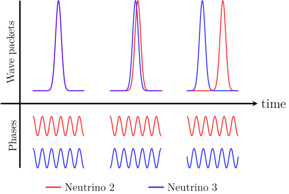
Figure 3.1: Physics of oscillations illustrated with the $\mathup{{{\nu}}{}_{\scriptstyle{\!\mu}}}$–$\mathup{{{\nu}}{}_{\scriptstyle{\!\tau}}}$ system. We assume the existence of two mass components $\nu_{2}$ and $\nu_{3}$, indicated in red and blue respectively. The the arrow indicates the direction of the time. We display the wave packets — plots over the arrow — and the phases of the two mass components — plots below the arrow — at three representative times. 1. Initially (left), the two wavepackets are overlapped; until the two mass components are in phase, the state is $|\mathup{{{\nu}}{}_{\scriptstyle{\!\mu}}}\rangle$. 2. Then (middle), the two wavepackets are still overlapped; when the two mass components get counter-phased, the state becomes $|\mathup{{{\nu}}{}_{\scriptstyle{\!\tau}}}\rangle$. 3. After a long time (right), when the mass components are fully separated, we have a 50/50 flavor mixture.

Discussion of the formula

Neutrino masses enter (3.46) or equivalently (3.47) through the energy $E_{j}=\sqrt{p^{2}+m^{2}_{j}}$ and the velocity $v_{j}=p/E_{j}$. Thus, they produce two kinds of effects: the relative phases get different after a time $(E_{1}-E_{2})t_{\mathrm{osc}}\sim 1$ and the wave packets separate after a time $(v_{1}-v_{2})t_{\mathrm{dec}}\sim\sigma_{z}$, where $\sigma_{z}$ is the size of the wave packet. These are two different effects: interferences connected to the phase change, namely neutrino oscillations and separation of the wave packets, namely decoherence. It is important to stress that oscillations occur when the components of the wave packet associated to the different mass states overlap. Using $\sigma_{E}\approx c\,\sigma_{p}\sim c/\sigma_{z}$, we have,

$$t_{\mathrm{osc}}\sim t_{\mathrm{dec}}\times\frac{\sigma_{E}}{E}$$ (3.48)

Therefore, if the energy uncertainty $\sigma_{E}$ is much less than the value of the energy $E\approx pc$, neutrino oscillations will happen earlier and decoherence will happen later.

Equivalently, we can carry on the discussion by introducing and comparing three lengths: propagation length (i.e., distance between production and detection) $L=c\,t$; oscillation length $L_{\mathrm{osc}}=c\,t_{\mathrm{osc}}$; coherence length $L_{\mathrm{dec}}=c\,t_{\mathrm{dec}}$. Similarly, it is useful to note the two phenomena mentioned above corresponds to different velocities among the individual components: oscillations are caused by the difference among phase velocities $E_{j}/p$; decoherence is caused by the difference among group velocities $\mathrm{d}E_{j}/\mathrm{d}p=p/E_{j}$ instead.

Summary and illustration

At this point we have a general picture of what happens to ultrarelativistic neutrinos during their propagation:

1. The light neutrinos are produced according to the mixing matrix, since we assume that their kinetic energy is much larger than their mass.

2. Initially, we can assume in excellent approximation that the components with different masses, and thus also their wave packets, travel with velocity $c$. Thus it is appropriate to use $\mathcal{G}(z-ct)$ for all mass components in (3.46) or (3.47). Then, we rewrite (3.47) as follows,

   $$[\Psi^{\ell}]_{\ell^{\prime}}=\mathcal{U}_{\ell\ell^{\prime}}(t)\ \mathcal{G}(z-ct)$$ (3.49)

   and we see that the last, flavor independent factor, that describes the shape of the wave-function, is multiplied by the usual transition amplitude

   $$\mathcal{U}_{\ell\ell^{\prime}}(t)=U_{\ell j}^{*}\,e^{i(pz-E_{j}t)}\,U_{\ell^{\prime}\!j}$$ (3.50)

   The key feature of this phase is that the differences of phases $(E_{i}-E_{j})t$ deviate from zero and oscillations in proper sense occur.

3. Subsequently, the differences of phases of the components $(E_{i}-E_{j})t$ appearing in $\mathcal{U}_{\ell\ell^{\prime}}$ become very large. Thus, the phase factors oscillate very rapidly when we vary, even slightly, the distance or the energy at the source or at the detection. For this reason, the effect of the oscillatory terms is not anymore measurable in practice.

4. Eventually, the wave packets separate and the description becomes even simpler conceptually. When the different components do not overlap anymore, oscillations are completely lost (i.e., not only for practical purposes). Interestingly, neutrinos with different masses could be in principle detected separately in this stage even if, in practice, this is extremely difficult. If they are not measured, the probability of transmutation that follow from step $2^{\prime}.$ and step 3. are the same.

The steps 1., 2. and 3. are illustrated graphically in Figure 3.1.

Section 3.2 Applications and examples

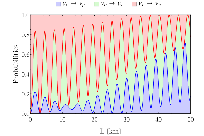
Figure 3.2: In this plot we consider an electron neutrino of $3\text{\,}\mathrm{MeV}$ that propagates for several kilometers. For each fixed distance, the probability that the electron neutrino becomes a muon (or tau) neutrino in the course of the propagation is given by the blue (or green) region. The probability that it remains an electron neutrinos is given by the red region. The plot emphasizes that the sum of the three probabilities is one, i.e., there is no loss of probability.

We will proceed to illustrate the formulae given above by considering several specific applications and particular cases. However, we would like to begin simply by justifying better the name of “oscillations” given to this phenomenon, especially in the modern literature. We have seen the appearance of a several oscillatory functions, however this point is illustrated much better by a plot. In Figure 3.2, we show the probabilities that an electron neutrino remains such or changes in the course of its propagation, with the parameters given in Table 2.1.

3.2.1 Why two flavor formulae are so useful

Two flavor oscillation formulae in vacuum allow us to discuss the main facts concerning the observed neutrino oscillations. In order to see how, recall that: 1. electron antineutrinos are produced in nuclear fission reactors and then detected; similarly 2. muon neutrinos are produced by charged pion decays (either naturally or artificially) and then detected.

In both cases, we are interested in the probability of survival. Let us consider,

$$|\mathup{{\overline{{\nu}}}{}_{\scriptstyle{\!e}}}\rangle=U_{\mathrm{e}i}|\bar{\nu}_{i}\rangle\quad\text{and}\quad|\mathup{{{\nu}}{}_{\scriptstyle{\!\mu}}}\rangle=U_{\mu i}^{*}|{\nu}_{i}\rangle$$ (3.51)

When the distances are not too large, as quantified below, only the third neutrino, the one that has the larger mass difference with the other two states, causes oscillations. The other two neutrinos mass states have effectively the same mass. In other words, the discussion of Section 3.1.2 applies to the real situations, due to the value of the oscillation parameters given in Table 2.1. Let us recall the amplitudes of oscillations of interest, namely,

$$\langle\mathup{{\overline{{\nu}}}{}_{\scriptstyle{\!e}}}|\mathup{{\overline{{\nu}}}{}_{\scriptstyle{\!e}}},t\rangle=\sum_{i=1}^{3}|U_{\mathrm{e}i}|^{2}e^{-iE_{i}t}\approx e^{-iE_{1}t}\left[1-|U_{\mathrm{e}3}|^{2}+|U_{\mathrm{e}3}|^{2}e^{i(E_{3}-E_{1})t}\right]$$ (3.52)

where we used the above assumption, along with unitarity. The two flavor formulae follow,

$$P_{\overline{\nu}_{\!\;\!\mbox{\tiny e}}\to\overline{\nu}_{\!\;\!\mbox{\tiny e}}} = 1-4|U_{\mathrm{e}3}^{2}|\left(1-|U_{\mathrm{e}3}^{2}|\right)\sin^{2}\varphi$$ (3.53)

$$P_{\nu_{\mbox{\tiny$\mu$}}\to\nu_{\mbox{\tiny$\mu$}}} = 1-4|U_{\mu 3}^{2}|\left(1-|U_{\mu 3}^{2}|\right)\sin^{2}\varphi$$ (3.54)

and adopting the standard parameterization ((2.38) and Table 2.1) we can replace,

$$|U_{\mathrm{e}3}|=\sin\theta_{13}\quad\text{and}\quad|U_{\mu 3}|=\cos\theta_{13}\sin\theta_{23}$$ (3.55)

Using these simple formulae, Daya Bay and Reno collaborations (reactor experiments) measured $\theta_{13}\sim 9^{\circ}$; Super-Kamiokande and MACRO (atmospheric neutrino experiments) and subsequently K2K and MINOS (accelerator experiments) measured $\theta_{23}\sim 45^{\circ}$. Due to the fact that $\Delta m^{2}_{31}\approx$2.5\text{\times}{10}^{-3}\text{\,}{\mathrm{eV}}^{2}$$, oscillations manifested in these experiments, and indeed the phases in the conditions of these experiments are large enough,

$$\small\varphi=1.267\;\frac{\Delta m^{2}_{31}L}{E_{\nu}}\approx 1\quad\text{if}\quad\begin{cases}L=$1\text{\,}\mathrm{km}$,\ E_{\nu}=$3\text{\,}\mathrm{MeV}$&\small\text{[reactor $\nu$]}\\ L=$700\text{\,}\mathrm{km}$,\ E_{\nu}=$2\text{\,}\mathrm{GeV}$&\small\text{[long baseline]}\\ \end{cases}$$ (3.56)

The average value of the electron survival probability for solar neutrinos, that follows from the above formula including the effect of $\theta_{13}$ is, is $\langle P_{\nu_{\mbox{\tiny e}}\to\nu_{\mbox{\tiny e}}}\rangle=\langle P_{\overline{\nu}_{\!\;\!\mbox{\tiny e}}\to\overline{\nu}_{\!\;\!\mbox{\tiny e}}}\rangle=1-(\sin^{2}2\theta_{13})/2=0.95$: this is too small to account for solar neutrino disappearance. In fact, it is the effect of the splitting between the other two mass states that explains solar neutrinos! This hypothesis was tested by KamLAND reactor experiments at distances of the order of $L\sim$100\text{\,}\mathrm{km}$$, that determined precisely $\Delta m^{2}_{21}\approx$7.4\text{\times}{10}^{-5}\text{\,}{\mathrm{eV}}^{2}$$ using the formula,

$$P_{\overline{\nu}_{\!\;\!\mbox{\tiny e}}\to\overline{\nu}_{\!\;\!\mbox{\tiny e}}}=\sin^{4}\theta_{13}+\cos^{4}\theta_{13}(1-\sin^{2}2\theta_{12}\sin^{2}\phi)$$ (3.57)

where this time $\phi=1.267\,\Delta m^{2}_{21}\,L/E_{\nu}$. The value of the last angle, that describes the composition of $\nu_{e}$ in terms of the last two mass states, is $\theta_{12}\approx 33^{\circ}$. The ambiguity $\theta_{12}\leftrightarrow 90^{\circ}-\theta_{12}$ due to the occurrence of $\sin^{2}2\theta_{12}$ in the formula is resolved by high energy solar neutrinos, that are affected by matter (MSW) effect and will be discussed in the next section.

The above considerations show that, despite their simplicity, the two-flavor formulae (or their direct extensions) allow us to understand a great deal of facts concerning the evidences of neutrinos oscillations. See Table 2.1 for an updated summary of the values of the oscillation parameters.

3.2.2 A special case: maximal mixing

Definitions

The cases of maximal mixing are of special interest. We begin the discussion with the two flavor case. One assumes that a pair of neutrinos, say $\mu$ and $\tau$, is described by,

$$|\mathup{{{\nu}}{}_{\scriptstyle{\!\mu}}}\rangle=\frac{|\nu_{1}\rangle+|\nu_{2}\rangle}{\sqrt{2}}\quad\text{and}\quad|\mathup{{{\nu}}{}_{\scriptstyle{\!\tau}}}\rangle=\frac{-|\nu_{1}\rangle+|\nu_{2}\rangle}{\sqrt{2}}$$ (3.58)

namely,

$$|\nu_{\ell}\rangle=U_{\ell i}^{*}|\nu_{i}\rangle\quad\text{with}\quad U=\frac{1}{\sqrt{2}}\left(\begin{array}[]{cc}+1&+1\\ -1&+1\end{array}\right)$$ (3.59)

so that the mixing elements satisfy $|U_{\ell i}|^{2}=1/2$. This simple case is a good approximation of some situations of physical interest. The maximal mixing in the $3\times 3$ case is a bit more intricate. It is based on the assumption that the mixing matrix is,

$$U=\frac{1}{\sqrt{3}}\left(\begin{array}[]{ccc}1&1&1\\ 1&\omega&\omega^{2}\\ 1&\omega^{2}&\omega\\ \end{array}\right)\quad\text{where}\quad\omega=e^{i\;2\;\pi/3}$$ (3.60)

so that $\omega^{3}=1$ and all matrix elements satisfy $|U_{\ell i}|^{2}=1/3$. This case is to be thought as a toy model since it does not correspond to any situation of physical reality but it is anyway useful as test bed, in particular to better understand CP violating phenomena. In fact, we find $J_{\mathrm{CP}}=\mbox{Im}[U_{\mathrm{e}1}U_{\mu 1}^{*}U_{\mathrm{e}2}^{*}U_{\mu 2}]=1/(6\sqrt{3})$, namely, the maximal amount of CP violation, as discussed after (2.44). In fact, it can be checked by direct calculation that, by adopting a suitable redefinition of phases as in (2.22), the mixing matrix given in (3.60) is equivalent to the standard form given in (2.38) with the values $\theta_{12}=\theta_{23}=\pi/4$, $\sin\theta_{13}=1/\sqrt{3}$ and $\delta=+\pi/2$.

Two flavor case

Using the oscillation probability of (3.6) and the definition of maximal mixing, it is easy to show that,

$$P_{\mu\tau}=P_{\tau\mu}=\sin^{2}\phi=1-P_{\mu\mu}=1-P_{\tau\tau}\quad\text{where}\quad\phi=\frac{\Delta m^{2}L}{4E}$$ (3.61)

Thus:

1. the probabilities of appearance and disappearance are all connected;

2. the averaged values are $\langle P_{\ell\ell^{\prime}}\rangle=1/2$ for $\ell,\ell^{\prime}=\mu,\tau$;

3. it is possible that the original type of neutrino fully disappears, when $\phi=\pi/2$.

Three flavor case

We recall that (by definition) all matrix elements satisfy $|U_{\ell i}|^{2}=1/3$; moreover, it is interesting to impose also the additional condition,

$$\phi=\phi_{21}=\phi_{32}=\phi_{31}/2$$ (3.62)

or equivalently $\Delta m^{2}=m_{2}^{2}-m_{1}^{2}=m_{3}^{2}-m_{2}^{2}=(m_{3}^{2}-m_{1}^{2})/2$. This is a rather particular case that is not realized in nature but has some didactic interest for what concerns CP (or better T) violation. We have,

$$P_{\ell\ell}=\frac{(1+2\cos\phi)^{2}}{9}\quad\text{and}\quad P_{\ell\ell^{\prime}}=\frac{1-P_{\ell\ell}}{2}+\frac{2\;\xi}{3\sqrt{3}}\sin\phi\,(1-\cos\phi)$$ (3.63)

where $\ell\neq\ell^{\prime}$. The last term describes CP-violation and the sign $\xi$ is,

$$\xi=-1\quad\text{for}\quad\ell\ell^{\prime}=\mathrm{e}\mu,\mu\tau,\tau e\quad\text{and}\quad\xi=+1\quad\text{for}\quad\ell\ell^{\prime}=\mu\mathrm{e},\tau\mu,\mathrm{e}\tau$$ (3.64)

It is noticeable that when $\phi=2\pi/3$ we have,

$$\left(\begin{array}[]{ccc}P_{\mathrm{e}\mathrm{e}}&P_{\mathrm{e}\mu}&P_{\mathrm{e}\tau}\\ P_{\mu\mathrm{e}}&P_{\mu\mu}&P_{\mu\tau}\\ P_{\tau\mathrm{e}}&P_{\tau\mu}&P_{\tau\tau}\end{array}\right)=\left(\begin{array}[]{ccc}0&0&1\\ 1&0&0\\ 0&1&0\end{array}\right)$$ (3.65)

therefore, the chosen combination of mixing angles and of phases of oscillations produces the maximum possible deviation from the case when the oscillation probability is symmetric, $P_{\ell\ell^{\prime}}=P_{\ell^{\prime}\ell}$. In other words, this is the maximum amount of T violation, that is, the maximum difference between the cases when $\nu_{\ell}\to\nu_{\ell^{\prime}}$ and $\nu_{\ell^{\prime}}\to\nu_{\ell}$ with $\ell\neq\ell^{\prime}$.

3.2.3 A 2 flavor case of oscillations with neutrino interactions

When we have muon and tau neutrinos of high energies we should consider the fact that they oscillate, approximatively with maximal mixing $\theta_{\mbox{\tiny max}}=45^{\circ}$, and, also, they interact (differently) with matter. (This is relevant, for example, for the neutrinos produced in the center of the Sun due to the annihilation or decay of hypothetical dark matter particles [13].) After charged current interactions, neutrinos convert into the corresponding charged leptons that are eventually slowed down and absorbed. This can be formally described including an imaginary term in the hamiltonian, that accounts for their disappearance at the original energy. Thus,

$$H=U(\theta_{\mathrm{max}})\left(\begin{array}[]{cc}-\kappa&0\\ 0&\kappa\end{array}\right)U^{-1}(\theta_{\mathrm{max}})-\frac{i}{2}\left(\begin{array}[]{cc}\Gamma_{\mu}&0\\ 0&\Gamma_{\tau}\end{array}\right)$$ (3.66)

with,

$$\kappa=\frac{\Delta m^{2}}{4E}$$ (3.67)

and where $\Gamma_{\mu,\tau}$ are the interaction rates with matter. Setting,

$$\Gamma=\frac{\Gamma_{\mu}+\Gamma_{\tau}}{2}\qquad\gamma=\frac{\Gamma_{\mu}-\Gamma_{\tau}}{4}$$ (3.68)

we get the convenient form of the hamiltonian,

$$H=\left(\begin{array}[]{cc}-i\gamma&\kappa\\ \kappa&+i\gamma\end{array}\right)-\frac{i\Gamma}{2}\left(\begin{array}[]{cc}1&0\\ 0&1\end{array}\right)$$ (3.69)

In the case of constant density, we can easily calculate the evolutor $\mathcal{U}=\exp(-iHr)$, where $r$ is the distance travelled by the neutrino, proceeding as follows. The second part, proportional to the unit matrix, is trivially exponentiated. For the rest, let us begin by assuming the parameter $\gamma$ as imaginary. The resulting matrix is hermitian and can be easily diagonalized. Its eigenvalues $\lambda_{\pm}$ and mixing angles are,

$$\lambda_{\pm}=\pm\alpha\ ,\ \cos 2\theta=\frac{i\gamma}{\alpha},\ \sin 2\theta=\frac{\kappa}{\alpha}\quad\text{where}\quad\alpha=\sqrt{\kappa^{2}-\gamma^{2}}$$ (3.70)

At this point, it is easy to exponentiate the full hamiltonian. The result is,

$$\mathcal{U}=e^{-\Gamma r/2}\left(\begin{array}[]{cc}\cos\varphi-\frac{\gamma}{\alpha}\sin\varphi&-i\frac{\kappa}{\alpha}\sin\varphi\\ -i\frac{\kappa}{\alpha}\sin\varphi&\cos\varphi+\frac{\gamma}{\alpha}\sin\varphi\end{array}\right)\quad\text{with}\quad\varphi=\alpha r$$ (3.71)

Finally, we use analytical continuation to come back to the case when $\gamma$ is real, i.e., the case in which we are actually interested. We find the explicit formula for $\mathup{{{\nu}}{}_{\scriptstyle{\!\mu}}}\to\mathup{{{\nu}}{}_{\scriptstyle{\!\tau}}}$ conversion,

$$P_{\nu_{\mbox{\tiny$\mu$}}\to\nu_{\mbox{\tiny$\tau$}}}=\frac{e^{-r\,\Gamma}}{1-\varepsilon^{2}}\ \sin^{2}\!\left(\displaystyle\frac{\Delta m^{2}\;r}{4\;E_{\nu}}\sqrt{1-\varepsilon^{2}}\right)\quad\text{with}\quad\varepsilon=\frac{\Gamma_{\mu}-\Gamma_{\tau}}{\Delta m^{2}/E_{\nu}}$$ (3.72)

It is possible to find in Ref. [13] the numerical values of the interaction rates $\Gamma$ and more discussion of this and similar situations.

3.2.4 Electron survival probability in three flavors

The electron survival probability in the full three flavor regime contains an imprint of the type of mass hierarchy. The goal of the future experiment JUNO is just to probe this effect, see Ref. [14] for a very detailed discussion. Here we derive the oscillation probability and demonstrate this effect. The formal manipulations are slightly more demanding than the previous ones and for this reason we use a brief and special notation. The oscillation amplitude for $\mathup{{\overline{{\nu}}}{}_{\scriptstyle{\!e}}}\to\mathup{{\overline{{\nu}}}{}_{\scriptstyle{\!e}}}$ in 3 flavors is,

$$\mathcal{U}_{3} =e^{-iE_{3}t}\left[C_{12}C_{13}\,e^{if_{31}}+S_{12}C_{13}\,e^{if_{32}}+S_{13}\right]$$ (3.73)

$$=e^{-iE_{3}t}\left[C_{13}\;\mathcal{U}_{2}+S_{13}\right]$$

where the corresponding expression in 2 flavor (or, if $\theta_{13}=0$) is,

$$\mathcal{U}_{2}=C_{12}\,e^{if_{31}}+S_{12}\,e^{if_{32}}$$ (3.74)

and where we simplified the notation by using the standard parameterization and setting,

$$C_{ij}=\cos^{2}\theta_{ij},\ S_{ij}=\sin^{2}\theta_{ij}\quad\text{and}\quad f_{ij}=(E_{i}-E_{j})t\approx\frac{m_{i}^{2}-m_{j}^{2}}{2E}L$$ (3.75)

In this manner we get,

$$P_{3} =C_{13}^{2}|\mathcal{U}_{2}|^{2}+S_{13}^{2}+2\,C_{13}S_{13}\,\mbox{Re}[\mathcal{U}_{2}]$$ (3.76)

$$=C_{13}^{2}P_{2}+S_{13}^{2}+2\,C_{13}S_{13}\,{\mbox{Re}[\mathcal{U}_{2}]}$$

where we set by definition,

$$P_{2}=|\mathcal{U}_{2}|^{2}\quad\text{and}\quad P_{3}=|\mathcal{U}_{3}|^{2}$$ (3.77)

The piece in which we are mostly interested is,

$$\mbox{Re}[\mathcal{U}_{2}]=C_{12}\cos(f_{31})+S_{12}\cos(f_{32})$$ (3.78)

The two large phases of oscillations, that is $f_{31}$ and $f_{32}$, differ but only by a small amount. This is given by the phase of the ‘solar’ (or better KamLAND’s) neutrino oscillations,

$$f_{31}-f_{32}=f_{21}\equiv f$$ (3.79)

It is convenient to introduce a special choice of the common part of the large phase factor $\Phi$, such that the slow and the fast oscillations get neatly separated. This choice is [15],

$$f_{31}=\alpha\,\Phi+S_{12}\,f\quad\text{and}\quad f_{32}=\alpha\,\Phi-C_{12}\,f$$ (3.80)

where $\alpha=\pm 1$ corresponds to normal/inverse hierarchy, respectively. In fact, we have,

$$\mbox{Re}\left[\mathcal{U}_{2}\right]= C_{12}\cos\left(\Phi+\alpha S_{12}\,f\right)+S_{12}\cos\left(\Phi-\alpha C_{12}\,f\right)=$$ (3.81)

$$= \cos\Phi\ \left[\ C_{12}\cos(S_{12}\,f)+S_{12}\cos(C_{12}\,f)\right]+$$

$$-\alpha\sin\Phi\;\left[\ C_{12}\sin\left(S_{12}\,f\right)-S_{12}\sin\left(C_{12}\,f\right)\right]$$

This expression is consistent with the following definition of $\varphi$,

$$\begin{array}[]{l}\cos\varphi\ |\mathcal{U}_{2}|\equiv C_{12}\cos\left(S_{12}\,f\right)+S_{12}\cos\left(C_{12}\,f\right)\\ \sin\varphi\ |\mathcal{U}_{2}|\equiv C_{12}\sin\left(S_{12}\,f\right)-S_{12}\sin\left(C_{12}\,f\right)\end{array}$$ (3.82)

This special definition allows us to recast the term of interest in a very neat manner,

$${\mbox{Re}\left[\mathcal{U}_{2}\right]}={|\mathcal{U}_{2}|}\times\cos\left(\Phi+\alpha\varphi\right)$$ (3.83)

In this manner, we have separated the effects of the fast and the slow oscillations in the terms ${\mbox{Re}[\mathcal{U}_{2}]}$: the phase $\Phi$ is large and produces the fast oscillations, whereas the phase $\varphi$ is small, and varies only with the solar phase $f$, just as the term $|\mathcal{U}_{2}|=\sqrt{P_{2}}$.

Summarizing, our expression for the electron antineutrino survival probability is,

$$P_{3} =C_{13}^{2}|\mathcal{U}_{2}|^{2}+S_{13}^{2}+2\,C_{13}S_{13}\,\mbox{Re}[\mathcal{U}_{2}]$$ (3.84)

$$=C_{13}^{2}P_{2}+S_{13}^{2}+2\,C_{13}S_{13}\sqrt{P_{2}}\cos(\Phi+\alpha\varphi)$$

The last terms shows that in the region of $\Phi$-driven fast oscillations, the prediction of the two mass hierarchies are slightly ‘out of tune’ between them; the detection of this effect requires a very good energy resolution. Moreover, the overall factor $S_{13}=\sin^{2}\theta_{13}$ suppresses this effect, which contributes to make the task of JUNO demanding.

3.2.5 The limit of fully averaged oscillations

An important limiting case is when we have vacuum oscillations and the phases of oscillation are very large. In this case, the oscillatory (cosinusoidal) terms get averaged to zero in any practical situation: e.g., when the production or the detection points are not perfectly known, when there is a distribution of initial energies and this is not perfectly measured in the detector, etc. The case is known as averaged oscillations and sometimes also as Gribov-Pontecorvo regime [16]. Strictly speaking, one cannot speak of ‘oscillations’ in proper sense. However, this case is of wide physical interest: for instance, it is important for low energy solar neutrinos (when ‘matter effects’ are negligible) or also for high energy neutrino from cosmic sources, as those that have been plausibly measured with IceCube.

The formulae for averaged oscillations are very simple and were given in Ref. [17],

$$P_{\nu_{\ell}\to\nu_{\ell^{\prime}}}=P_{\bar{\nu}_{\ell}\to{\bar{\nu}}_{\ell^{\prime}}}=\sum_{i=1}^{3}|U_{\ell i}|^{2}|U_{\ell^{\prime}i}|^{2}$$ (3.85)

Of course the averaged probabilities are subject to unitarity constraints as any other set of oscillation probabilities, e.g.: $\sum_{\ell^{\prime}=\mathrm{e},\mu,\tau}P_{\nu_{\ell}\to\nu_{\ell^{\prime}}}=1$, or just as the elements of the mixing matrix squared $|U_{\ell i}|^{2}$. However, owing to the symmetry in the exchange $\ell\leftrightarrow\ell^{\prime}$, the averaged probabilities depend only upon three parameters, and not four as $|U_{\ell i}|^{2}$. The probabilities can be arranged in a symmetric matrix,

$$\mathcal{P}=\left(\begin{array}[]{ccc}\frac{1}{3}+2P_{0}&\frac{1}{3}-P_{0}+P_{1}&\frac{1}{3}-P_{0}-P_{1}\\ &\frac{1}{3}+\frac{P_{0}}{2}-P_{1}+P_{2}&\frac{1}{3}+\frac{P_{0}}{2}-P_{2}\\ &&\frac{1}{3}+\frac{P_{0}}{2}+P_{1}+P_{2}\end{array}\right)$$ (3.86)

where we introduced 3 new parameters, that can be expressed in terms of the usual ones as follows,

$$P_{0} = \frac{1}{2}\left\{(1-\epsilon)^{2}\left[1-\frac{\sin^{2}2\theta_{12}}{2}\right]+\epsilon^{2}-\frac{1}{3}\right\}$$ (3.87)

$$P_{1} = \frac{1-\epsilon}{2}\left\{\gamma\cos 2\theta_{12}+\beta\frac{1-3\epsilon}{2}\right\}$$ (3.88)

$$P_{2} = \frac{1}{2}\left\{\gamma^{2}+\frac{3}{4}\beta^{2}(1-\epsilon)^{2}\right\}$$ (3.89)

and the small quantities $\alpha,\beta,\gamma,\epsilon$ (only the last one is known to date) are,

$$\begin{cases}\epsilon=\sin^{2}\theta_{13}\\ \alpha=\sin\theta_{13}\cos\delta\sin 2\theta_{12}\sin 2\theta_{23}\\ \beta=\cos 2\theta_{23}\\ \displaystyle\gamma=\alpha-\frac{\beta}{2}\cos 2\theta_{12}(1+\epsilon)\end{cases}$$ (3.90)

It is interesting that the averaged oscillation probabilities depend upon the CP-violating phase and also upon the departure of $\theta_{23}$ from $45^{\circ}$, through $\cos 2\theta_{23}$. However, there are only 3 free parameters, thus one combination of the usual parameters is degenerate. More precisely $P_{0}$ is well known; $P_{1}$ contains most uncertainties; $P_{2}$ is positive and very small. The above results are taken from Ref. [18], where further discussion, references, applications and numerical results can be found.

Chapter 4 Neutrino oscillations in matter

In this section, we introduce and discuss the matter term of Wolfenstein. Then we present a few analytical solutions of the equation of propagation, including the one discussed by Mikheyev and Smirnov. The aim is to illustrate the characteristic features of oscillations due to the matter term. Finally, we consider some physical applications.

Section 4.1 The matter (or Wolfenstein) term

4.1.1 Origin

Vacuum oscillations are caused by the relative phases that the components of a neutrino with given flavor obtain in the course of the time $t$. This is a typical undulatory or quantum phenomenon, as it is evident from the connection between energies $E_{i}$ of each component and the frequencies of oscillation $\nu_{i}$ of each component: $E_{i}=h\,\nu_{i}$. Indeed, as we have shown in Section  3.1.4, vacuum oscillations can be described by an effective hamiltonian. In this section we discuss a new point: electron neutrinos that propagate in a material medium receive a special, additional phase of scattering, as first remarked by Wolfenstein. We can think to this new phase as an additional term in the hamiltonian of propagation, or also as a flavor-specific refraction term.

Consider the scattering amplitude of neutrinos onto electrons at rest and more specifically consider the case when the neutrino momentum is unchanged (=forward scattering),

$$\nu_{\ell}(\vec{p}\,)\ \mathup{{{e}}^{\scriptstyle{-}}}\to\nu_{\ell}(\vec{p}\,)\ \mathup{{{e}}^{\scriptstyle{-}}}$$ (4.1)

This amplitude of scattering is maximum when $\ell=\mathup{{{e}}}$, due to charged current interactions. Thus, electronic neutrinos receive a special phase, that contributes to the effective hamiltonian and eventually also to oscillations. Also neutral currents give an additional phase due to the forward scattering of neutrinos with any particle $X$ of the medium (excepting neutrinos themselves) $\nu_{\ell}(\vec{p}\,)X\to\nu_{\ell}(\vec{p}\,)X$: however this contribution is the same for all types of neutrinos and therefore it contributes only to an irrelevant overall phase factor for all neutrinos.

The most important case when this new phase is relevant is when the matter, where neutrinos propagate, contains electrons at rest or almost at rest. We will focus the subsequent discussion on this case. However, in principle, one can have also effects due to polarization, to collective motions, etc.

4.1.2 Formal derivation of the matter term

We are interested to describe the contribution of Fermi interactions to the forward scattering of an electron neutrino. The idea is to evaluate the amplitude of forward scattering in terms of the matrix element of the hamiltonian. Thus, we need a formal description of the hamiltonian, of the state of the neutrino and of the state of the medium. We show how to derive, under reasonable assumptions, the standard result (namely, the Wolfenstein or matter term).

Fermi hamiltonian for neutrino-electron interaction

The hamiltonian density of the Fermi interactions contains the following interaction between electrons and electron neutrinos,

$$\mathcal{H}_{\nu_{\mathrm{e}\mathrm{e}}}^{\mathrm{cc}}=+\frac{G_{\mathrm{F}}}{\sqrt{2}}\ \bar{\nu}_{\mathrm{e}}\gamma_{a}(1-\gamma_{5})\mathrm{e}\ \bar{\mathrm{e}}\gamma^{a}(1-\gamma_{5})\nu_{\mathrm{e}}$$ (4.2)

where $G_{\mathrm{F}}>0$ whose sign is predicted by the standard electroweak model. This implies the following hamiltonian, written in terms of relativistic quantum fields,

$$\mathbf{H}_{\nu_{\mathrm{e}\mathrm{e}}}^{\mathrm{cc}}=\sqrt{2}\,G_{\mathrm{F}}\int\mathrm{d}^{3}x\ \bar{\nu}_{\mathrm{eL}}\gamma_{a}\nu_{\mathrm{eL}}\ \bar{\mathrm{e}}\gamma^{a}(1-\gamma_{5})\mathrm{e}$$ (4.3)

where:

1. we have integrated over the space coordinates to pass from the hamiltonian density to the hamiltonian operator;

2. we have introduced the chiral projector $P_{\mathrm{L}}=(1-\gamma_{5})/2$ and defined $\nu_{\mathrm{e}\mathrm{L}}=P_{\mathrm{L}}\nu_{\mathrm{e}}$;

3. we have applied the Fierz transformation described in Section A.3.

Matrix element for forward scattering

Let us consider the previous hamiltonian at a given time, say, $t=0$. Then, we consider its matrix element between the same initial and final state $|s\rangle$, namely,

$$\langle s|\mathbf{H}_{\nu_{\mathrm{e}\mathrm{e}}}^{\mathrm{cc}}(t=0)|s\rangle\quad\text{with}\quad|s\rangle=|\nu_{\mathrm{e}},{\mathrm{e}}_{1},{\mathrm{e}}_{2},{\mathrm{e}}_{3}\dots\rangle$$ (4.4)

The state $|s\rangle$ describes a single electron neutrino, localized around $\vec{x}=\vec{x}_{0}$, and a large number of electrons almost at rest, localized around the positions $\vec{x}=\vec{x}_{i}$ with $i=1,2,3,\dots$ (we have in mind a neutrino propagating in the matter e.g. of the Sun or of the Earth). The only operator containing the electron fields that has large matrix elements is the time component of the vectorial part $\bar{\mathrm{e}}\gamma_{0}\mathrm{e}={\mathrm{e}}^{\dagger}\mathrm{e}$, that is the electron density operator. Thus, the relevant part of the matrix element is,

$$\langle s|\mathbf{H}_{\nu_{\mathrm{e}\mathrm{e}}}^{\mathrm{cc}}(t=0)|s\rangle=\sqrt{2}\,G_{\mathrm{F}}\int\mathrm{d}^{3}x\ \langle s|\ \mathbf{n}_{\mathrm{e}}(\vec{x})\ \mathbf{n}_{{\nu}_{\mathrm{e}\mathrm{L}}}(\vec{x})\ |s\rangle$$ (4.5)

where we indicate the density operators of the electron and of the neutrino with $\mathbf{n}_{\mathrm{e}}(\vec{x})={\mathrm{e}}^{\dagger}\!(0,\vec{x}){\mathrm{e}}(0,\vec{x})$ and $\mathbf{n}_{{\nu}_{\mathrm{e}\mathrm{L}}}(\vec{x})={{\nu}_{\mathrm{e}\mathrm{L}}}^{\dagger}\!(0,\vec{x}){\nu}_{\mathrm{e}\mathrm{L}}(0,\vec{x})$. We factorize the state $|s\rangle$ and consider separately the matrix elements of the two operators. We have,

$$\langle{\nu}_{\mathrm{e}\mathrm{L}}|\mathbf{n}_{{\nu}_{\mathrm{e}\mathrm{L}}}(\vec{x})|{\nu}_{\mathrm{e}\mathrm{L}}\rangle = |\Psi_{{\nu}_{\mathrm{e}\mathrm{L}}}(\vec{x},\vec{x}_{0})|^{2}$$ (4.6)

$$\langle{\mathrm{e}}_{1},{\mathrm{e}}_{2},{\mathrm{e}}_{3}\dots|\mathbf{n}_{\mathrm{e}}(\vec{x})|{\mathrm{e}}_{1},{\mathrm{e}}_{2},{\mathrm{e}}_{3}\dots\rangle = \sum_{i}|\Psi_{e}(\vec{x},\vec{x}_{i})|^{2}$$ (4.7)

where we have introduced the wave-functions of the neutrino and of the electrons, emphasizing the position of each particle. We supposed for simplicity that the electrons are distributed similarly, but around different positions.

In the case of interest, the individual electrons are distributed in small cells, e.g., atomic sizes of $\sigma_{\mathrm{e}}\sim$1\text{\times}{10}^{-8}\text{\,}\mathrm{cm}$$, whereas the neutrino is distributed in a much larger scale $\sigma_{\nu}$. Another important quantity is the macroscopic electron density that we denote by $n_{\mathrm{e}}(\vec{x})$. We suppose that the scale of variation of the macroscopic electron density, $\Delta r_{e}$ is much larger than the size of the neutrino wave-function. For the Sun, e.g., this is $\Delta r_{\mathrm{e}}\sim R_{\odot}/10$ and also in the Earth it is typically km size or more. Summarizing, we suppose that,

$$\Delta r_{\mathrm{e}}\gg\sigma_{\nu}\gg\sigma_{\mathrm{e}}$$ (4.8)

In the above assumptions we can evaluate the integral in (4.5). We divide the region where the neutrino wave-function is non-zero in many cubes $a=1,2,3\dots$. Each cube has size $\Delta x$ such that $\sigma_{\nu}\gg\Delta x\gg\sigma_{\mathrm{e}}$ and volume $\Delta x^{3}$. In each cube there are a lot of electrons, while the neutrino density is almost constant with value $|\Psi_{{\nu}_{\mathrm{e}\mathrm{L}}}(\vec{x}_{a},\vec{x}_{0})|^{2}$. If we integrate the electron density in the cube with label $a$, we have $\int_{a}\mathrm{d}^{3}x\sum_{i}|\Psi_{\mathrm{e}}(\vec{x},\vec{x}_{i})|^{2}=N_{\mathrm{e}}(\vec{x}_{a})\gg 1$, namely the number of electrons inside the cube. This is almost the same for all $a$, because we suppose that $\Delta r_{\mathrm{e}}\gg\Delta x$. We can then approximate: $N_{\mathrm{e}}(\vec{x}_{a})\approx n_{\mathrm{e}}(\vec{x}_{0})\Delta x^{3}$, where we indicate the position $\vec{x}_{0}$ of the neutrino since we are interested in the value of the electronic density where the neutrino is. Thus, the integral is,

$$I(\vec{x}_{0})=\int\mathrm{d}^{3}x\sum_{i}|\Psi_{\mathrm{e}}(\vec{x},\vec{x}_{i})|^{2}\times|\Psi_{{\nu}_{\mathrm{e}\mathrm{L}}}(\vec{x},\vec{x}_{0})|^{2}$$ (4.9)

which can be solved as,

$$I(\vec{x}_{0}) \approx\sum_{a}N_{\mathrm{e}}(\vec{x}_{a})|\Psi_{{\nu}_{\mathrm{e}\mathrm{L}}}(\vec{x}_{a},\vec{x}_{0})|^{2}\approx$$ (4.10)

$$\approx n_{\mathrm{e}}(\vec{x}_{0})\sum_{a}\Delta x^{3}\ |\Psi_{{\nu}_{\mathrm{e}\mathrm{L}}}(\vec{x}_{a},\vec{x}_{0})|^{2}\approx$$

$$\approx n_{\mathrm{e}}(\vec{x}_{0})\times\int\mathrm{d}^{3}x\ |\Psi_{{\nu}_{\mathrm{e}\mathrm{L}}}(\vec{x},\vec{x}_{0})|^{2}=n_{\mathrm{e}}(\vec{x}_{0})$$

Therefore, the matrix element of interest, for a single neutrino located around $\vec{x}=\vec{x}_{0}$, is just,

$$\langle\mathbf{H}_{\nu_{\mathrm{e}\mathrm{e}}}^{\mathrm{cc}}\rangle=\sqrt{2}G_{\mathrm{F}}\ n_{\mathrm{e}}(\vec{x}_{0})$$ (4.11)

Following the above derivation, it is easy to see that an electron antineutrino has the same matrix element but with the opposite sign, due to the fact that the operator $\mathbf{n}_{\nu_{\mathrm{e}\mathrm{L}}}$ counts the net number of electron neutrinos: therefore, an antineutrino counts $-1$.

4.1.3 Hamiltonians of propagation including the matter term

Thus, we should add to the $3\times 3$ vacuum hamiltonians, that describe free neutrino/antineutrino propagation, also the matter hamitonian that acts on flavor states,

$$H_{\mathrm{MSW}}=\pm\sqrt{2}\,G_{\mathrm{F}}n_{\mathrm{e}}(\vec{x})\left(\begin{array}[]{ccc}1&0&0\\ 0&0&0\\ 0&0&0\end{array}\right)\quad\text{where}\quad\begin{cases}+&\text{for $\nu$}\\ -&\text{for $\bar{\nu}$}\end{cases}$$ (4.12)

where $\vec{x}$ is the position of the neutrino and $n_{\mathrm{e}}(\vec{x})$ the number density of electrons. To be sure, note that this term has the right dimension, namely “energy”, since the Fermi constant has $1/\text{energy}^{2}$ and the electron density is $1/\text{volume}=\text{energy}^{3}$ in natural units. Note that we consider a linear contribution in the Fermi constant (whereas cross sections or decay widths depend upon $G_{\mathrm{F}}^{2}$). This fact shows that we are considering amplitudes and/or wave-functions rather than probabilities and witnesses the quantum nature of the phenomenon. A last remark is in order: this new term can be regarded as a contribution to the refraction of the electronic neutrino wave.

Summarizing, the flavor of ultrarelativistic neutrinos of given energy $E$ that propagate in a medium with electronic density $n_{\mathrm{e}}(x)$, changes according to neutrino and antineutrino hamiltonians that have one part due to vacuum oscillations and another one due to the Wolfenstein (or matter) term. For neutrinos, this is given by,

$$H_{\nu}=U^{*}\,\mathrm{diag}(k)\,U^{t}+V(x)\,\mathrm{diag}(1,0,0)$$ (4.13)

where the symbols $U^{*}$ and $U^{t}$ indicate the complex conjugate and the transpose of the mixing matrix, respectively, and where,

$$k_{i} = m_{i}^{2}/(2E)$$ (4.14)

$$V(x) \equiv \sqrt{2}G_{\mathrm{F}}n_{\mathrm{e}}(x)$$ (4.15)

For antineutrinos we need to replace,

$$U\to U^{*}\quad\text{and}\quad V\to-V$$ (4.16)

We have adopted a shorthand $k$ for the quantity that describes the effect that are purely due to neutrino masses (i.e., of vacuum oscillations).

Before discussing some specific example and some solutions, we note that these hamiltonians contain the energy $E=pc$ (and/or the momentum) of the neutrino and its position $x$, too. This description might seem to be in contradiction with the Heisenberg indetermination principle, i.e., with some basic facts of quantum mechanics. However, as we have discussed above, neither of these observable is exactly measured. The idea is that, in actual circumstances, neutrinos travel in wave packets, which are supposed to be non dispersive.

4.1.4 Remarks

Numerical value

The numerical value of the matter term and of the vacuum term, given in the same units of inverse meter, is,

$$V = \sqrt{2}\,G_{\mathrm{F}}n_{\mathrm{e}}=\frac{3.868\times 10^{-7}}{\mathrm{m}}\times\frac{n_{\mathrm{e}}}{\mathrm{mol}/\mathrm{cm}^{3}}$$ (4.17)

$$k = \frac{\Delta m^{2}}{2E}=\frac{2.533}{\mathrm{m}}\times\frac{\Delta m^{2}}{\mathrm{eV}^{2}}\times\frac{\mathrm{MeV}}{E}$$ (4.18)

Let us remark that, when the matter term is small in comparison to the other one, we reduce to the case of vacuum oscillations. In order to clarify when this happens, let us examine the ratio of these two terms. We find,

$$\frac{V}{k}\equiv\frac{\sqrt{2}\;G_{\mathrm{F}}n_{\mathrm{e}}}{\Delta m^{2}/(2E)}\approx\left(\frac{\rho\ Y_{\mathrm{e}}}{100\,\mathrm{mol}/\mathrm{cm}^{3}}\right)\left(\frac{8\times 10^{-5}\,\mathrm{eV}^{2}}{\Delta m^{2}}\right)\left(\frac{E}{5\,\mathrm{MeV}}\right)$$ (4.19)

where $\rho$ is the mass density and $Y_{\mathrm{e}}$ is the fraction of electrons and/or of protons (since ordinary matter is neutral). The values of the parameters are those needed to interpret solar neutrino data: 1. the central density of the Sun is expected to be about $150\,\mathrm{g}/\mathrm{cm}^{3}$, with some fraction of Helium; 2. the numerical value of $\Delta m^{2}$ is close to the one given in Table 2.1; 3. the energy thresholds of Super-Kamiokande and SNO are close to $5\text{\,}\mathrm{MeV}$. The comparison in (4.19) shows that at low neutrino energies $E\ll$5\text{\,}\mathrm{MeV}$$, the matter (Wolfenstein) term has a negligible effect whereas at high energy it is relevant.

A comment on CP and T violation

Let us compare the dependence of certain probabilities of conversion in various cases,

$$P_{\nu_{\mbox{\tiny$\mu$}}\to\nu_{\mbox{\tiny e}}}= F(U,V;E_{\nu},L)$$ (4.20)

$$P_{\overline{\nu}_{\!\;\!\mbox{\tiny$\mu$}}\to\overline{\nu}_{\!\;\!\mbox{\tiny e}}}= F(U^{*},-V;E_{\nu},L)$$

$$P_{\nu_{\mbox{\tiny e}}\to\nu_{\mbox{\tiny$\mu$}}}= F(U^{*},V;E_{\nu},L)$$

$$P_{\overline{\nu}_{\!\;\!\mbox{\tiny e}}\to\overline{\nu}_{\!\;\!\mbox{\tiny$\mu$}}}= F(U,-V;E_{\nu},L)$$

where $F$ is a certain function. When we exchange the initial and final state, we consider T-reversal which implies $U\neq U^{*}$. Furthermore, we see that there are also C and CP violating effects when we exchange particles and antiparticles, that should be attributed to the exchange $V\to-V$. In fact, ordinary matter contains electrons, and therefore, it induces C and CP violating effects in the neutrino propagation that are of ‘environmental nature’, on top of the CP (or T) violating effects of fundamental nature, due to the fact that the leptonic mixing matrix is complex.

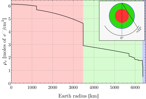
Figure 4.1: Density profile of the Earth according to the PREM model [19]. Different colors correspond to different Earth layers: 1. inner ad outer core in red; 2. mantle in green; and 3. crust in blue. Visualizing the shell structure in scale, we notice that a neutrino can cross the core only if its angle is smaller than $\approx 32^{\circ}$.

Amplitude of three flavor neutrino oscillations

In order to obtain a general expression for the oscillation amplitude in matter in the three flavor case, we can consider the mixing matrix $U=R_{23}\ \Delta\ R_{13}\ \Delta^{*}\ R_{12}$, given in (2.39), such that the propagation hamiltonian in (4.13) is,

$$H_{\nu}=R_{23}\ \Delta\ \tilde{H}\ \Delta^{*}\ R_{23}^{\mathrm{t}}$$ (4.21)

with,

$$\tilde{H}=R_{13}\ R_{12}\ \mathrm{diag}(k)\ R_{12}^{\mathrm{t}}\ R_{13}^{\mathrm{t}}+V(x)\mathrm{diag(1,0,0)}$$ (4.22)

where $\tilde{H}$ is independent on $\theta_{23}$ and $\delta$. The formal expression of the amplitude of the three flavor neutrino oscillations when the matter effect is included, can be hence written as,

$$\mathcal{U}=\mathrm{Texp}\left[-i\int\mathrm{d}t\;{H}_{\nu}(t)\right]\equiv R_{23}\Delta\left(\begin{array}[]{ccc}u_{11}&u_{12}&u_{13}\\ u_{21}&u_{22}&u_{23}\\ u_{31}&u_{32}&u_{33}\end{array}\right)\Delta^{*}R_{23}^{\mathrm{t}}$$ (4.23)

where $u_{ij}$ depend upon $\Delta m^{2}_{23}$, $\theta_{13}$, $\Delta m^{2}_{12}$, $\theta_{12}$ and on the type of mass hierarchy (normal/inverted), that can be easily fixed changing a discrete parameter $h=\pm 1$. When we solve the evolution equations with a certain assumption on the matter density, we calculate the complex numbers $u_{ij}$ and therefore the amplitudes and the probabilities of oscillations. For example, at the web address,

http://pcbat1.mi.infn.it/~battist/cgi-bin/oscil/index.r

the interface of the ‘Neutrino Oscillations Simulator’ allows the user to plot and to download the probabilities for neutrinos or antineutrinos that propagate from two points on the surface of the Earth. The solutions are obtained numerically, as described in Ref. [20], see in particular Eqs. (1), (3), (5), (6) there and using the Preliminary reference Earth model (PREM) of the electronic Earth density illustrated in Figure 4.1.

Section 4.2 Analytical solutions of the equations of propagation

For a generic profile of electronic density, it is always possible to resort to numerical methods to solve the equations of propagations. However, the solutions have an oscillatory character and this makes the problem difficult; we need to use a sufficiently small step, that can be eventually time consuming.

However, there are various cases when the propagation equations have exact or approximate analytical solutions, that are useful to describe the physics. We will discuss two of them in the following. The first is simply the case when we have a constant density; this can be applied in sequence to layers of constant density, finding eventually the overall amplitude. The second case instead is when the density varies slowly, which is called the adiabatic case; this admits a simple solution, which moreover is physically important.

4.2.1 Constant matter density and ‘resonance’

The case when we have two flavors ($2\times 2$ matrices) and matter with constant density is particularly instructive. We have,

$$U(\theta)=\left(\begin{array}[]{cc}c&s\\ -s&c\end{array}\right)\quad\text{and}\quad k\equiv{k_{2}-k_{1}}=\frac{\Delta m^{2}}{2E}$$ (4.24)

where we can assume $\Delta m^{2}>0$ and $0<\theta<\pi/2$.

Note that, for the description of oscillations, it is harmless if the hamiltonian of propagation is modified by adding a real constant: in fact, this constant yields the same phase for all flavor states, that is irrelevant for the flavor transformations. Thus, let us choose the constant in such a manner that our hamiltonian is traceless, i.e., let us subtract the term $-\mathrm{tr}(H)/2\cdot\mathbb{1}$, getting,

$$H=\frac{k}{2}\,U\,\mathrm{diag}(-1,1)\ U^{\mathrm{t}}+\frac{V}{2}\,\mathrm{diag}(1,-1)=\frac{1}{2}\left(\begin{array}[]{cc}V-kc_{2}&ks_{2}\\ ks_{2}&kc_{2}-V\end{array}\right)$$ (4.25)

where we use the obvious shorthands $c_{2}=\cos 2\theta$ and $s_{2}=\sin 2\theta$.

At this point, we can simply redefine the angles and the parameters $k$, in such a manner that this hamiltonian coincides formally with a vacuum hamiltonian. This is obtained by setting,

$$\begin{cases}kc_{2}-V\equiv k_{m}c_{2m}\\ ks_{2}\equiv k_{m}s_{2m}\end{cases}\quad\Longleftrightarrow\quad\begin{cases}\displaystyle t_{2m}=\frac{s_{2}}{c_{2}-V/k}\\ k_{m}=k\sqrt{s_{2}^{2}+(c_{2}-V/k)^{2}}\end{cases}$$ (4.26)

In this manner, we can just reinterpret the solutions, that have been already obtained for the case of vacuum oscillations. We need only to examine the so called mixing angle in matter $\theta_{m}$ and the parameter $k_{m}\equiv\Delta m^{2}_{m}/(2E)$.

Let us discuss the most interesting feature. Suppose that $V>0$ (as it is usually the case) and $kc_{2}$ has the same sign (namely, suppose $\theta<\pi/4$). By varying the energy of the neutrino $E$, we vary $k$ from $0$ to $\infty$. Thus, it is always possible to realize the case $c_{2m}=0$, namely, the case when $\theta_{m}=\pi/4$ (maximal mixing). This case is called resonance and the corresponding energy is called the resonance energy. The resonance point corresponds to the minimum splitting between the energy levels of the mass eigenstates. The possibile transition between the two energy levels (let us call them $\lambda_{\pm}$) is usually defined level crossing. From (4.26) is evident that the minimum distance between $\lambda_{\pm}=\pm k_{m}/2$ occurs for $V=kc_{2}$. Note that: 1. this is possible whichever the value of the mixing angle in vacuum; 2. at the resonance energy, also $k_{m}$ and thus $\Delta m^{2}_{m}$ get the minimum value.

Summarizing, we will have three limiting situations for neutrinos,

$$\begin{cases}V\ll k&\Rightarrow\theta_{m}\approx\theta\\ V=kc_{2}&\Rightarrow\theta_{m}\approx 45^{\circ}\\ V\gg k&\Rightarrow\theta_{m}\approx 90^{\circ}\\ \end{cases}$$ (4.27)

while for the antineutrinos instead, the sign of $V$ will be opposite and the mixing angle in matter will be smaller than the one in vacuum. We leave to the interested Reader a complete study of $\Delta m^{2}_{m}$, $\theta_{m}$ and $P_{\mathrm{e}\mu}(k_{m},\theta_{m})$, as the parameter $V$ is varied.

4.2.2 Adiabatic propagation / MSW effect

Generally, as the neutrino proceeds along its path, the electron density varies. The case when the variation is slow (in a sense to be made precise later) is particularly important and in this case it is possible to obtain a solution of the equations of propagation. This is called the adiabatic solution. Let us proceed step by step:

1. First of all we rewrite the hamiltonian, by introducing the local eigenvalues. We rewrite,

   $$i\partial_{t}\nu=[\,U_{m}\,\mathrm{diag}(k_{m})\,U_{m}^{\dagger}\,]\ \nu$$ (4.28)

   where $\nu$ is the vector of the flavor states, $\nu=(\mathup{{{\nu}}{}_{\scriptstyle{\!e}}},\mathup{{{\nu}}{}_{\scriptstyle{\!\mu}}},\mathup{{{\nu}}{}_{\scriptstyle{\!\tau}}})^{\mathrm{t}}$, while $U_{m}$ is the mixing matrix that depends upon the position and/or the time along the path.

2. Now we introduce the local mass eigenstates $n=(n_{1},n_{2},n_{3})^{\mathrm{t}}$,

   $$\nu\equiv U_{m}n\;\Rightarrow\;i\partial_{t}n=[\mathrm{diag}(k_{m})-i(U_{m}^{\dagger}\partial_{t}U_{m})]n$$ (4.29)

   If the second term was not there, it would be easy to solve the problem.

3. In order to understand the physics, we focus from here on the $2\times 2$ case, when all matrices are real and say $\nu=(\mathup{{{\nu}}{}_{\scriptstyle{\!e}}},\mathup{{{\nu}}{}_{\scriptstyle{\!\mu}}})^{\mathrm{t}}$ and $n=(n_{1},n_{2})^{\mathrm{t}}$. After a few direct calculations, we find that the propagation equation is,

   $$i\partial_{t}\left(\begin{array}[]{c}n_{1}\\ n_{2}\end{array}\right)=\left(\begin{array}[]{cc}-k_{m}/2&\quad-i\partial_{t}\theta_{m}\\ i\partial_{t}\theta_{m}&\quad k_{m}/2\end{array}\right)\left(\begin{array}[]{c}n_{1}\\ n_{2}\end{array}\right)$$ (4.30)

   where the effect of the change in the electron density is contained in $\partial_{t}\theta_{m}$.

4. Now we introduce the definition,

   $$\quad\text{Adiabaticity parameter:}\quad\gamma=\left|\frac{2\dot{\theta}_{m}}{k_{m}}\right|$$ (4.31)

   and we call ‘adiabatic condition’ the one when $\gamma$ is always small, so that the new term is negligible and we can easily read the solution. In order to have a more precise idea, we note that the case when $k_{m}$ is minimum, i.e., at the ‘resonance’, the adiabaticity parameter is,

   $$V(x_{\mathrm{res}})=kc_{2}\;\Rightarrow\;\gamma(x_{\mathrm{res}})=\left|\frac{\dot{V}}{V}\ \frac{c_{2}}{k\;s_{2}^{2}}\right|$$ (4.32)

   The case when the condition of adiabaticity is violated significantly is a bit more complex. However, it can be still treated analytically, and the effects are described by a negative exponential in the parameter $1/\gamma$.

5. Suppose that $\gamma$ is small. The local mass eigenstates $n_{1}$ and $n_{2}$ will not change and evolve only getting a phase,

   $$n_{1}(t)=e^{i\xi}\ n_{1}(0)\quad n_{2}(t)=e^{-i\xi}\ n_{2}(0)\quad\text{where}\quad\xi=\int\frac{k_{m}}{2}\mathrm{d}t$$ (4.33)

   This is the formal statement that describes the case of ‘adiabatic propagation’ in our two flavor system. At this point it is easy to find the propagation amplitude, e.g., $\mathcal{U}_{\mathrm{e}\to\mathrm{e}}=cc_{m}e^{i\xi}+ss_{m}e^{-i\xi}$ (In order to derive this equation, we begin from $\nu=U_{m}n$, we find that $\mathup{{{\nu}}{}_{\scriptstyle{\!e}}}=c_{m}n_{1}+s_{m}n_{2}$ and then we calculate $\mathup{{{\nu}}{}_{\scriptstyle{\!e}}}(t)$ using $n_{1}(t)$ ed $n_{2}(t)$, thanks to the linearity of the equation; finally, we use the definition, $\mathcal{U}_{\mathrm{e}\to\mathrm{e}}=\langle\mathup{{{\nu}}{}_{\scriptstyle{\!e}}},\mathup{{{\nu}}{}_{\scriptstyle{\!e}}}(t)\rangle$, or in other words we take the scalar product).

6. Since the phases $\xi$ are large, we can average to zero the interference terms in the formulae of the probability of electron survival, getting,

   $$P_{\mathrm{e}\mathrm{e}}=c^{2}c_{m}^{2}+s^{2}s_{m}^{2}$$ (4.34)

   this is the formula that is usually employed and in which we are interested. We recall that the case when the interference terms drop out is a typical classical average. In the three flavor case the obvious generalization is $P_{\mathrm{e}\mathrm{e}}=|U_{\mathrm{e}i}^{2}||U^{m}_{\mathrm{e}i}|^{2}$ and will be discussed in the last part of this section.

7. For practical purposes, it is useful to note that when $V\gg k$, the electron neutrino is $\mathup{{{\nu}}{}_{\scriptstyle{\!e}}}\approx n_{2}$, since, as just explained, it propagates in matter with the combination $\mathup{{{\nu}}{}_{\scriptstyle{\!e}}}(t)=c_{m}n_{1}(t)+s_{m}n_{2}(t)$ and for $V\gg k$, $\theta_{m}\approx 90^{\circ}$, as discussed in Section  4.2.1. Since the central density in the Sun is about $150\text{\,}\mathrm{g}\text{\,}{\mathrm{cm}}^{-3}$, this is a good approximation for the propagation of solar neutrinos above about $5\text{\,}\mathrm{MeV}$.

Let us note that the above description is strictly analogous to the situation of a two-level hamiltonian that depends upon one parameter. This analogy can help to understand the propagation in the adiabatic regime, as discussed below.

Time dependent hamiltonian in adiabatic approximation

Let us consider a time dependent hamiltonian and introduce the eigenstates and eigenvalues

$$H(t)|n(t)\rangle=E_{n}(t)|n(t)\rangle$$ (4.35)

and suppose the hamiltonian is not degenerate.

Let us derive w.r.t. time,

$$\dot{H}|n\rangle+H\dot{|n\hphantom{|}}\rangle=\dot{E_{n}}|n\rangle+E_{n}\dot{|n\hphantom{|}}\rangle$$ (4.36)

then we multiply by $\langle m|$ with $n\neq m$,

$$\mathrm{l.h.s.} =\langle m|\dot{H}|n\rangle+\langle m|H\dot{|n\hphantom{|}}\rangle=\langle m|\dot{H}|n\rangle+E_{m}\langle m\dot{|n\hphantom{|}}\rangle$$ (4.37)

$$\mathrm{r.h.s.} =\dot{E_{n}}\langle m|n\rangle+E_{n}\langle m\dot{|n\hphantom{|}}\rangle=E_{n}\langle m\dot{|n\hphantom{|}}\rangle$$

so we find,

$$\langle m\dot{|n\hphantom{|}}\rangle=\frac{\langle m|\dot{H}|n\rangle}{E_{n}-E_{m}}\quad\text{if}\quad n\neq m$$ (4.38)

Thus the eigenstate acquires overlap with other eigenstates if the derivative of $H$ is large in comparison to the energy differences.

Instead in the case $n=m$ we have,

$$\langle n|n\rangle=1\>\Rightarrow\>\dot{\langle n\hphantom{\rangle}}|n\rangle+\langle n\dot{|n\hphantom{|}}\rangle=0\>\Rightarrow\>\langle n\dot{|n\hphantom{|}}\rangle=-\langle n\dot{|n\hphantom{|}}\rangle^{*}$$ (4.39)

in other words, this number is imaginary. We define,

$$\eta_{n}=i\langle n\dot{|n\hphantom{|}}\rangle\in\mathbb{R}$$ (4.40)

Now we can write the generic states as,

$$|\psi\rangle=\sum_{n}e^{-iS_{n}}c_{n}|n\rangle\quad\text{where}\quad S_{n}(t)=\int_{0}^{t}d\tau\ E_{n}(\tau)$$ (4.41)

Its time evolution is dictated by the Schrödinger equation $i\dot{|\psi\rangle}=H|\psi\rangle$, that implies,

$$\sum_{n}\dot{S_{n}}e^{-iS_{n}}c_{n}|n\rangle+i\sum_{n}\left(e^{-iS_{n}}\dot{c}_{n}|n\rangle+e^{-iS_{n}}c_{n}\dot{|n\hphantom{|}}\rangle\right)$$ (4.42)

$$= \sum_{n}e^{-iS_{n}}c_{n}H\,|n\rangle$$

the first and last term cancel out. Multiplying by $\langle m|$, we have

$$\dot{c}_{m}=-\sum_{n}e^{i(S_{m}-S_{n})}c_{n}\langle m\dot{|n\hphantom{|}}\rangle=-c_{m}\langle m\dot{|m\hphantom{|}}\rangle-\sum_{n\neq m}e^{i(S_{m}-S_{n})}c_{n}\langle m\dot{|n\hphantom{|}}\rangle$$ (4.43)

Using the above result,

$$\dot{c}_{m}=-c_{m}\langle m\dot{|m\hphantom{|}}\rangle-\sum_{n\neq m}c_{n}\ \frac{\langle m|\dot{H}|n\rangle}{E_{n}-E_{m}}e^{i(S_{m}-S_{n})}$$ (4.44)

If the second term is negligible, namely in the adiabatic case, we have,

$$c_{m}(t)=c_{m}(0)\exp\left[i\int_{0}^{t}\mathrm{d}\tau\ \eta_{m}(\tau)\right]$$ (4.45)

namely, $|c_{m}|^{2}$ does not change with time.

From the time evolution of the mass eigenstates in (4.30), we have,

$$i\partial_{x}n_{2}=\frac{k_{m}}{2}\left(i\frac{2\dot{\theta}_{m}}{k_{m}}n_{1}+n_{2}\right)=\frac{k_{m}}{2}\left(i\gamma n_{1}+n_{2}\right)$$ (4.46)

where $\gamma$ is the adiabatic parameter in (4.31). Since in the adiabatic approximation the limit $\gamma\ll 1$ holds, the mass eigenstate time evolution is,

$$\begin{cases}i\;\partial_{x}n_{1}=-k_{m}\,n_{1}/2\\ i\;\partial_{x}n_{2}=k_{m}\,n_{2}/2\end{cases}$$ (4.47)

i.e. the time evolutions (time and spatial evolutions are equivalent in the relativistic regime) of the two eigenstates are independent one from another. As a consequence, in the adiabatic approximation, if $\mathup{{{\nu}}{}_{\scriptstyle{\!e}}}\approx n_{2}$ in the production point (e.g. for solar neutrinos), $\mathup{{{\nu}}{}_{\scriptstyle{\!e}}}$ remains in that eigenstate during all the adiabatic evolution.

To summarize, the case of adiabatic propagation applies if the probability of transition between the two eigenstates is always negligible, even when the two levels get as close as possible without crossing each other (a sub-case called “avoided crossing” in quantum mechanics).

Effect of the Earth on neutrino propagation

As we have just seen, in the case of solar $\mathup{{{\nu}}{}_{\scriptstyle{\!e}}}$ we expect to receive on Earth just the mass eigenstate $\nu_{2}$ above a certain energy (adiabatic conversion). However, it is possible that neutrinos reach the detector passing through the Earth, i.e. in night time. Therefore, it is interesting to calculate the probability of conversions from $\nu_{2}$ to $\mathup{{{\nu}}{}_{\scriptstyle{\!e}}}$, in two flavors approximation. This has a very simple and useful expression in the case of constant matter density, that we discuss here.

In the two flavor basis, for the time independent hamiltonian in (4.25), the evolutor that describes the effect of the propagation in the Earth is,

$$\mathcal{U} =U_{m}\,\mathrm{diag}[e^{i\varphi_{m}},e^{-i\varphi_{m}}]\ U_{m}^{\mathrm{t}}$$ (4.48)

$$=\left(\begin{array}[]{cc}c_{m}+is_{m}\cos 2\theta_{m}&-is_{m}\sin 2\theta_{m}\\ -is_{m}\sin 2\theta_{m}&c_{m}-is_{m}\cos 2\theta_{m}\end{array}\right)$$

where $\varphi_{m}=\Delta m^{2}_{m}L/(4E)$, $c_{m}=\cos\varphi_{m}$, $s_{m}=\sin\varphi_{m}$. Consider the case of solar neutrinos; the initial state is $\nu_{2}$, that in flavor space is represented by $(\sin\theta,\cos\theta)$ and the final state is $\mathup{{{\nu}}{}_{\scriptstyle{\!e}}}$ that in flavor space is represented by $(1,0)$. The relevant matrix element of the evolutor is,

$$\mathcal{U}_{2\to\mathrm{e}} =(c_{m}+is_{m}\cos 2\theta_{m})\sin\theta-is_{m}\sin 2\theta_{m}\cos\theta$$ (4.49)

$$=c_{m}\sin\theta-is_{m}\sin(2\theta_{m}-\theta)$$

The last factor can be rewritten using the formulae for the mixing angles in matter,

$$\sin(2\theta_{m}-\theta)=\sin\theta\ \frac{1+\varepsilon}{\sqrt{(1+\varepsilon)^{2}-4\varepsilon\cos^{2}\theta}}$$ (4.50)

where as usual $\varepsilon=V/k=2EV/\Delta m^{2}$. With a bit of algebra, we obtain the desired result,

$$P_{\nu_{2}\to\nu_{\mbox{\tiny e}}}=|\mathcal{U}_{2\to\mathrm{e}}|^{2}=\sin^{2}\theta\left[1+{4\varepsilon\ \cos^{2}\theta}\ {\sin^{2}\left(\frac{\Delta m^{2}L}{4E}\xi\right)}\;/\;{\xi^{2}}\right]$$ (4.51)

with,

$${\xi}=\sqrt{(1+\varepsilon)^{2}-4\varepsilon\cos^{2}\theta}$$ (4.52)

where of course we have in mind the so-called “solar neutrino mass splitting” (the lowest one) and $\theta$ is in good approximation just $\theta_{12}\approx 33^{\circ}$.

Section 4.3 Applications and examples

4.3.1 High energy atmospheric neutrinos

In this section, taken from Ref. [23], we examine the oscillations of high energy atmospheric neutrinos. This is interesting, since one could discriminate the neutrino mass hierarchy by observing the details of the matter effect.

We begin by using some simplifying assumptions, postponing derivations and refinements. Let us consider oscillations with a single scale, and let us consider oscillations in constant matter density. In fact, the second hypothesis is rather inaccurate in the conditions in which we are interested for the experiments, and a more accurate evaluation of the oscillation probabilities for the actual calculations is required. However, a qualitative discussion based on simple-minded analytical results is sufficient to correctly understand the relevant features.

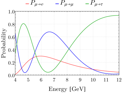
(a) Normal hierarchy.

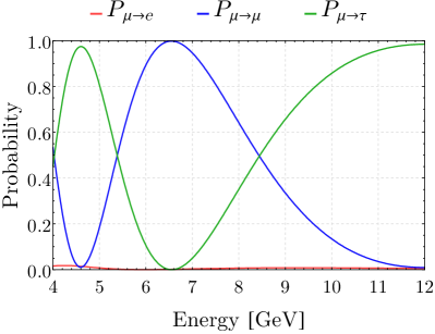
(b) Inverted hierarchy.

Figure 4.2: Oscillation probabilities in the Earth for a path of $L=7000\,\mathrm{km}$: the blue line is $P_{\nu_{\mbox{\tiny$\mu$}}\to\nu_{\mbox{\tiny$\mu$}}}$; the red line $P_{\nu_{\mbox{\tiny$\mu$}}\to\nu_{\mbox{\tiny e}}}$; the green one $P_{\nu_{\mbox{\tiny$\mu$}}\to\nu_{\mbox{\tiny$\tau$}}}$. The two panels refer to normal and inverted hierarchy respectively. The increase of $P_{\nu_{\mbox{\tiny$\mu$}}\to\nu_{\mbox{\tiny e}}}$ for normal hierarchy, due to matter effect, causes the decrease of $P_{\nu_{\mbox{\tiny$\mu$}}\to\nu_{\mbox{\tiny$\mu$}}}$.

Under the above assumptions, the probability that a muon neutrino converts into an electron neutrino is simply,

$$P_{\mu\mathrm{e}}=\sin^{2}\theta_{23}\;\sin^{2}2\widetilde{\theta_{13}}\;\sin^{2}\widetilde{\varphi}\quad\text{with}\quad\widetilde{\varphi}=\frac{\widetilde{\Delta m^{2}}L}{4E}$$ (4.53)

Most of the results in which we are interested follow from the above simple formula. In (4.53), we introduced the usual matter-modified mixing angle and squared-mass difference,

$$\begin{cases}\sin 2\widetilde{\theta_{13}}=\sin 2{\theta_{13}}\ /\Delta\\ \cos 2\widetilde{\theta_{13}}=(\cos 2{\theta_{13}}-\varepsilon)/\Delta\\ \widetilde{\Delta m^{2}}={\Delta m^{2}}\times\Delta\end{cases}$$ (4.54)

where,

$$\Delta=\pm\sqrt{(\cos 2\theta_{13}-\varepsilon)^{2}+\sin^{2}2\theta_{13}}$$ (4.55)

The sign of $\Delta$ is matter of convention; the ratio between matter and vacuum term is,

$$\varepsilon\equiv\pm\frac{\sqrt{2}G_{\mathrm{F}}n_{\mathrm{e}}}{\Delta m^{2}/(2E)}\approx\pm\frac{\rho}{$5.5\text{\,}\mathrm{g}\text{\,}{\mathrm{cm}}^{-3}$}\times\frac{Y_{\mathrm{e}}}{1/2}\times\frac{$2.4\text{\times}{10}^{-3}\text{\,}{\mathrm{eV}}^{2}$}{\Delta m^{2}}\times\frac{E}{$5.5\text{\,}\mathrm{GeV}$}$$ (4.56)

where $G_{\mathrm{F}}$ is the Fermi coupling and we identify $\Delta m^{2}$ with $\Delta m^{2}_{23}$. Now, instead, the sign is important: it is plus for normal hierarchy and minus for inverted hierarchy. Considering the average matter density of the Earth $\rho=$5.5\text{\,}\mathrm{g}\text{\,}{\mathrm{cm}}^{-3}$$ and $Y_{\mathrm{e}}=1/2$, we get $n_{\mathrm{e}}=1.7\times 10^{24}\mathup{{{e}}^{\scriptstyle{-}}}\mathrm{cm}^{-3}$ for the electronic density. Thus, the characteristic length of MSW theory is,

$$L_{*}\equiv\frac{1}{\sqrt{2}G_{\mathrm{F}}n_{\mathrm{e}}}\sim$1000\text{\,}\mathrm{km}$$$ (4.57)

We see that, for normal hierarchy, the maximum of $P_{\mu\mathrm{e}}$ is obtained when: 1. $\Delta$ is as small as possible, in order to maximize $\sin 2\widetilde{\theta_{13}}$; moreover 2. the phase of propagation is $\widetilde{\varphi}\sim\pi/2$. These conditions are met when the neutrino energy and the propagation distance are,

$$E_{\mathrm{max}}=\frac{\Delta m^{2}L_{*}}{2}\cos 2\theta_{13}\quad\text{and}\quad L_{\mathrm{max}}=\frac{\pi L_{*}}{\tan 2\theta_{13}}$$ (4.58)

or, numerically,

$$E_{\mathrm{max}}\sim$5.5\text{\,}\mathrm{GeV}$\quad\text{and}\quad L_{\mathrm{max}}\sim$9000\text{\,}\mathrm{km}$$$ (4.59)

In the case of inverted hierarchy, the matter effect depresses $P_{\mu\mathrm{e}}$, that becomes negligible.

As we have told, one would like to observe the matter effect. From the point of view of the experiments, one direct approach is to check the simple prediction concerning $P_{\mu\mathrm{e}}$. However, there are some practical advantages to detect muons rather than electrons. Then, let us consider the survival probability $P_{\mu\mu}$, focussing again on the normal hierarchy case. Let us discuss the case when the first local maximum of $P_{\mu\mu}$ is as small as possible. This results from $P_{\mu\tau}$ and from $P_{\mu\mathrm{e}}$, since $P_{\mu\mu}=1-P_{\mu\tau}-P_{\mu\mathrm{e}}$. We are interested in the case when the minimum of $P_{\mu\tau}$ happens in the vicinity of the energy identified in (4.59). When the phase of oscillation of $P_{\mu\tau}$ is close to the vacuum phase, the condition $\Delta m^{2}L/(2E_{\mathrm{max}})=2\pi$ gives $L\sim$6000\text{\,}\mathrm{km}$$. This suggests that the distance that amplifies the matter effect on $P_{\mu\mu}$ is between 6000 and $9000\text{\,}\mathrm{km}$, as confirmed by more complete analyses. These points are illustrated in Figure 4.2, that was obtained using the web interface mentioned in Section 4.1.4.

Description of atmospheric neutrino oscillations at various levels of accuracy

The general case requires a numerical solution based on (4.23). However, when the “solar” $\Delta m^{2}_{12}$ is set to zero — i.e., when its effects are negligible — the only non-zero out-of-diagonal elements $u_{ij}$ in (4.23) are $u_{13}$ and $u_{31}$. The CP violating phase $\delta$ drops out from the probabilities $P_{\ell\ell^{\prime}}=|\mathcal{U}_{\ell^{\prime}\ell}|^{2}$, that moreover becomes symmetric, $P_{\ell\ell^{\prime}}=P_{\ell^{\prime}\ell}$ for each $\ell,\ell^{\prime}=e,\mu,\tau$. Therefore, in this approximation we have 3 independent probabilities and all the other ones are fixed. We can choose, e.g.,

$$\begin{cases}P_{\mathrm{e}\mu}=\sin^{2}\theta_{23}|u_{13}|^{2}\\ P_{\mathrm{e}\tau}=\cos^{2}\theta_{23}|u_{13}|^{2}\\ P_{\mu\tau}=\sin^{2}\theta_{23}\cos^{2}\theta_{23}|u_{33}-u_{22}|^{2}\end{cases}$$ (4.60)

so that, e.g., $P_{\mathrm{e}\mathrm{e}}=1-P_{\mu\mathrm{e}}-P_{\tau\mathrm{e}}=|u_{11}|^{2}$. From these formulae we obtain,

$$P_{\mu\mathrm{e}}=\sin^{2}\theta_{23}\ (1-P_{\mathrm{e}\mathrm{e}})\quad\text{and}\quad P_{\mu\tau}=\frac{1}{4}\sin^{2}2\theta_{23}\left|1-\sqrt{P_{\mathrm{e}\mathrm{e}}}\ e^{i\hat{\varphi}}\right|^{2}$$ (4.61)

where $\hat{\varphi}$ is a (rapidly varying) phase factor. Two important remarks are in order:

1. The last equation shows that $P_{\mu\mathrm{e}}$ is large in the region where $P_{\mathrm{e}\mathrm{e}}$ is small, and that $P_{\mu\tau}$ remains close to zero in the first non-trivial minimum near $\hat{\varphi}=2\pi$, even when $P_{\mathrm{e}\mathrm{e}}\approx 0.3-0.4$ due to matter effect.

2. The sign of $\Delta m^{2}$ controls the sign of the vacuum hamiltonian; thus, switching between the two mass hierarchies or switching between neutrinos and antineutrinos has the same effect; e.g., $P_{\mathrm{e}\mu}(\text{IH})=P_{\bar{\mathrm{e}}\bar{\mu}}(\text{NH})$.

The first remark is consistent with our numerical findings, that $P_{\mu\mathrm{e}}$ is amplified and $P_{\mu\tau}$ does not deviate strongly from its behavior in vacuum in the conditions that are relevant for our discussion.

Proceeding further with the approximations, and considering at this point the case of constant matter density, we obtain simple and closed expressions. For the case of normal mass hierarchy, they read,

$$\begin{cases}u_{13}=u_{31}=-i\sin\widetilde{\varphi}\sin 2\widetilde{\theta_{13}}\\ u_{11}=\cos\widetilde{\varphi}+i\sin\widetilde{\varphi}\cos 2\widetilde{\theta_{13}}=u_{33}^{*}\\ u_{22}=\cos\widetilde{\varphi}^{\prime}+i\sin\widetilde{\varphi}\,^{\prime}\end{cases}$$ (4.62)

where,

$$\widetilde{\varphi}\,^{\prime}=\frac{{\Delta m^{2}}L}{4E}(1+\varepsilon)$$ (4.63)

From (4.60) and (4.62), we recover the expression of (4.53), used in the above discussion. In the approximation of constant matter density, the phase $\hat{\varphi}$ entering the expression of the probability $P_{\mu\tau}$ is given by $\sqrt{P_{\mathrm{e}\mathrm{e}}}\cos\hat{\varphi}\equiv\cos\widetilde{\varphi}\cos\widetilde{\varphi}\,^{\prime}-\sin\widetilde{\varphi}\sin\widetilde{\varphi}\,^{\prime}\cos 2\widetilde{\theta_{13}}$. This is close to the vacuum phase when $\varepsilon$ is large or small in comparison to 1: in fact, we have $\cos 2\widetilde{\theta_{13}}\sim\pm 1$ and $\widetilde{\varphi}\sim\pm\Delta m^{2}L/(4E)(1-\varepsilon)$ from (4.54), so that $\cos\hat{\varphi}\sim\cos[\Delta m^{2}L/(2E)]$.

4.3.2 Solar neutrinos

Let us discuss how the adiabatic solution applies to solar neutrinos. First of all, we note that the expected matter density profile is approximately exponential, $n_{\mathrm{e}}\propto\exp(-10x/R_{\odot})$, where $R_{\odot}=$7\text{\times}{10}^{8}\text{\,}\mathrm{m}$$ is the solar radius. Considering the mass difference squared, $\Delta m^{2}_{12}=$8\text{\times}{10}^{-5}\text{\,}{\mathrm{eV}}^{2}$$ and $\sin^{2}2\theta_{12}\sim 0.8$, (4.32) reads,

$$\gamma\approx\left|\frac{10\ c_{2}}{kR_{\odot}\ s_{2}^{2}}\right|\ll 1$$ (4.64)

for any possible relevant energy $E=0.1-$20\text{\,}\mathrm{MeV}$$. Thus, the local mass eigenstates $n_{1}$ and $n_{2}$ remain always such, just as described in (4.33); therefore, the result of (4.34) follows.

At this point we can interpret solar neutrinos. Let us begin by noting that we expect, a priori, that matter effects are important only for solar neutrinos of high energy, see (4.19). Given the density of electrons in the center of the Sun, $100\text{\,}\mathrm{mol}\text{\,}{\mathrm{cm}}^{-3}$, the mixing angle in matter is about $90^{\circ}$, see (4.27). Thus, since $s_{m}\approx 1$ and $c_{m}\approx 0$, the adiabatic formula for $P_{\mathrm{e}\mathrm{e}}$ simply becomes,

$$P_{\mathrm{e}\mathrm{e}}=\sin^{2}\theta_{12}$$ (4.65)

and there is no problem to explain the solar neutrino observations that indicate, at high energies, that the suppression factor of electron neutrinos is about 1/3. At this point, we know that the right solution is the one with $\theta_{12}\sim 30^{\circ}$ (since if we choose the other one that is allowed by vacuum neutrino oscillations, with $\theta_{12}\sim 60^{\circ}$, we would get 2/3 instead). Evidently, at low energies we recover the vacuum oscillation formula,

$$P_{\mathrm{e}\mathrm{e}}=1-\frac{\sin^{2}2\theta_{12}}{2}$$ (4.66)

In fact, making reference to the cases of (4.27), the limit $\theta\sim\theta_{m}$ applies.

4.3.3 Supernova neutrinos

Neutrinos from the gravitational collapse have energies from a few MeV to almost $100\text{\,}\mathrm{MeV}$, propagate at distances of the order of kpc and are produced in nuclear density regions, billion times larger than solar ones. They certainly undergo some oscillation effects. However, it is not clear, to date, to what extent it is possible to separate the effects of the oscillations from the astrophysical uncertainties since the latter ones are very large. We will limit ourselves to show here (without deriving them) a few basic formulas in view of the fact that this type of neutrinos do exist and are detectable.

First of all, we calculate the neutrino masses from the hamiltonian of propagation given in (4.13) as a function of the electron density. These masses depend upon the neutrino masses in vacuum, upon the energy of the neutrino, upon the electron density and upon the mixing angles $\theta_{12}$ and $\theta_{13}$ (see discussion in (4.23)). The result for the energy of a typical supernova neutrino is given in Figure 4.3 assuming the case of normal mass hierarchy. We see that if the density of electrons is large enough, we will have two “level crossing” or “resonances”. While in the case of solar neutrinos we had only one (of course, the one occurring for lowest densities), in the case of supernova we will have both of them, since in the center of the star (where the neutrinos are produced) we reach nuclear densities.

Then, we consider a generalization of the 2 flavors discussion of neutrino oscillations, given in Section 4.2.2. For generic values of the mixing angle $\theta$ and of the corresponding $\Delta m^{2}$, the matrix containing the probabilities of survival or of conversion, averaged over the large phases, is,

$$P=\left(\begin{array}[]{cc}c^{2}&s^{2}\\ s^{2}&c^{2}\end{array}\right)\left(\begin{array}[]{cc}1-P_{\mathrm{f}}&P_{\mathrm{f}}\\ P_{\mathrm{f}}&1-P_{\mathrm{f}}\end{array}\right)\left(\begin{array}[]{cc}c_{m}^{2}&s_{m}^{2}\\ s_{m}^{2}&c_{m}^{2}\end{array}\right)$$ (4.67)

The probability $P_{\mathrm{f}}$ is called flip probability and describes the possibility that there is a deviation from the relations given in (4.33). It is easy to verify that, in the limit $P_{\mathrm{f}}\to 0$, the above formula yields $P_{\mathrm{e}\mathrm{e}}$ as in (4.34). In fact, as we have checked in the case of solar neutrinos, the adiabaticity parameter $\gamma$ is very small, and this boils down in the conclusion that $P_{\mathrm{f}}\to 0$.

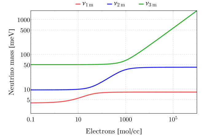
Figure 4.3: Neutrino masses calculated from the hamiltonian of propagation given in (4.13) and given as a function of the electron density for a typical energy of supernova neutrinos, $E_{\nu}=$20\text{\,}\mathrm{MeV}$$. We assumed normal mass hierarchy and fixed the lightest neutrino mass to be $m_{1}=$4\text{\,}\mathrm{meV}$$ just for illustration purposes.

The generalization to the 3 flavor case is quite direct, but requires to know the type of neutrino mass hierarchy. In fact, we know from the solar neutrino oscillations in matter that $\mathup{{{\nu}}{}_{\scriptstyle{\!e}}}$ is mostly in $\nu_{1}$, which corresponds to the choice of the angle $\theta_{12}$ discussed in the previous paragraph. Conversely, we still do not know for sure whether the neutrino $\nu_{3}$, that is responsible for atmospheric oscillations, is the heaviest (= direct or normal mass hierarchy) or the lightest (= inverse mass hierarchy), see Figure 2.1. Assuming the first case, that is slightly favored at present and it is also the most plausible theoretically, one finds [24],

$$\begin{array}[]{rl}P=&\left(\begin{array}[]{ccc}|U_{\mathrm{e}1}^{2}|&|U_{\mathrm{e}2}^{2}|&|U_{\mathrm{e}3}^{2}|\\ |U_{\mu 1}^{2}|&|U_{\mu 2}^{2}|&|U_{\mu 3}^{2}|\\ |U_{\tau 1}^{2}|&|U_{\tau 3}^{2}|&|U_{\tau 3}^{2}|\end{array}\right)\cdot\left(\begin{array}[]{ccc}1-P_{\mathrm{S}}&P_{\mathrm{S}}&0\\ P_{\mathrm{S}}&1-P_{\mathrm{S}}&0\\ 0&0&1\end{array}\right)\cdot\\[17.22217pt] &\left(\begin{array}[]{ccc}1&0&0\\ 0&1-P_{\mathrm{A}}&P_{\mathrm{A}}\\ 0&P_{\mathrm{A}}&1-P_{\mathrm{A}}\end{array}\right)\cdot\left(\begin{array}[]{ccc}|U_{\mathrm{e}1,m}^{2}|&|U_{\mu 1,m}^{2}|&|U_{\tau 1,m}^{2}|\\ |U_{\mathrm{e}2,m}^{2}|&|U_{\mu 2,m}^{2}|&|U_{\tau 3,m}^{2}|\\ |U_{\mathrm{e}3,m}^{2}|&|U_{\mu 3,m}^{2}|&|U_{\tau 3,m}^{2}|\end{array}\right)\end{array}$$ (4.68)

We see that now there are 2 flip probabilities. The first one is $P_{\mathrm{A}}$ connected to the “atmospheric” parameters (the delta mass squared $\Delta m^{2}_{23}$ and $\theta_{13}$) the second is $P_{\mathrm{S}}$ connected to the “solar” parameters (the delta mass squared $\Delta m^{2}_{12}$ and $\theta_{12}$). From this expression, we derive the electron survival probability,

$$P_{\mathrm{e}\mathrm{e}}=(1-P_{\mathrm{A}})|U_{\mathrm{e}3}^{2}|+P_{\mathrm{A}}\left[\ (1-P_{\mathrm{S}})|U_{\mathrm{e}2}^{2}|+P_{\mathrm{S}}|U_{\mathrm{e}1}^{2}|\ \right]$$ (4.69)

As in the case for solar neutrinos, we expect that $P_{\mathrm{S}}\sim 0$ also in the case of the supernova. The same is expected to be true for the other flip probability, $P_{\mathrm{A}}\sim 0$. Therefore, we conclude,

$$P_{\mathrm{e}\mathrm{e}}\sim|U_{\mathrm{e}3}^{2}|\sim 0$$ (4.70)

This implies that the electron neutrinos that we detect at Earth were produced at the source as muon or tau neutrinos.

It is possible to recap this conclusion with the help of Figure 4.3. Let us focus on the continuous (green) line, that shows the evolution of the heaviest mass eigenstate $\nu_{3m}$ from the vacuum (lower electronic densities) to the innermost part of the star (highest electronic densities). We note that after a certain density ($n_{\mathrm{e}}\sim$1000\text{\,}\mathrm{mol}\text{\,}{\mathrm{cm}}^{-3}$$) the mass of $\nu_{3m}$ increases linearly with the electron density (see Figure 4.3). In fact, the matter term in (4.13) is the largest part of the hamiltonian of propagation in the center of the star, it is linear in $n_{\mathrm{e}}$ and evidently the heaviest eigenstate of the matter term is just the electron neutrino. This means that an electron neutrino, produced in the center of the star, is just the heaviest mass eigenstate of the full hamiltonian in very good approximation, $|\nu_{\mathrm{e}}\rangle\approx|\nu_{3m}\rangle$. The adiabatic evolution implies that a neutrino follows the evolution of the mass eigenstate; in our case, the electron neutrino produced in the center of the star remains always the heaviest mass eigenstate, $|\nu_{\mathrm{e}}\rangle\approx|\nu_{3m}(t)\rangle$ for all times (up to an irrelevant overall phase) and exits from the star as $|\nu_{3}\rangle$. Thus, its survival probability is $|\langle\nu_{\mathrm{e}}|\nu_{3}\rangle|^{2}=|U_{\mathrm{e}3}^{2}|$.

4.3.4 Earth matter effect at solar and supernova energies

At solar neutrino energies, the probability $P_{\nu_{2}\to\nu_{\mathrm{e}}}$ given in (4.51) admits the simple numerical approximation

$$P_{\nu_{2}\to\nu_{\mathrm{e}}}\approx\displaystyle 0.3+1.7\%\ \kappa\ \sin^{2}\left(\frac{\Delta m^{2}L}{4E}\right)$$ (4.71)

with,

$$\kappa=\left(\frac{$7.37\text{\times}{10}^{-5}\text{\,}{\mathrm{eV}}^{2}$}{\Delta m^{2}}\right)\left(\frac{n_{\mathrm{e}}}{$2\text{\,}\mathrm{mol}\text{\,}{\mathrm{cm}}^{-3}$}\right)\left(\frac{E}{$5\text{\,}\mathrm{MeV}$}\right)$$ (4.72)

Therefore, we see that the detectors receive (slightly) more electron neutrinos in night than in day, which is the reason why this is called day-night effect or regeneration (adopting neutral kaon’s terminology). This feature remains true on average when we consider the full description of the Earth density.

Something similar is expected to happen in the case of supernova neutrinos. In this case the typical energy is $20-$30\text{\,}\mathrm{MeV}$$, larger than the one of solar neutrinos; thus, if neutrinos pass through the Earth, the effect is larger. In the approximation described above (Section 4.3.3), when we start from $\mathup{{{\nu}}{}_{\scriptstyle{\!e}}}$ we expect to receive on Earth $\nu_{3}$ (or $\nu_{2}$) for normal (or inverse) mass hierarchy; instead, $\mathup{{\overline{{\nu}}}{}_{\scriptstyle{\!e}}}$ becomes $\bar{\nu}_{1}$ (or $\bar{\nu}_{3}$). If we receive $\nu_{3}$ or $\bar{\nu}_{3}$, the relevant vacuum term (related to the larger value of $\Delta m^{2}$) is too large at these energies and no effect is expected. In the other cases, we can use almost immediately the above formula: in fact, we have the relation $P_{\nu_{1}\to\nu_{\mbox{\tiny e}}}=1-P_{\nu_{2}\to\nu_{\mbox{\tiny e}}}$, and we can obtain $P_{\bar{\nu}_{1}\to\overline{\nu}_{\!\;\!\mbox{\tiny e}}}$ from $P_{\nu_{1}\to\nu_{\mbox{\tiny e}}}$ by flipping the sign of the matter term: therefore, it is sufficient to calculate just one of these probabilities and we can immediately use the above result. Note the curious fact that $P_{\bar{\nu}_{1}\to\overline{\nu}_{\!\;\!\mbox{\tiny e}}}$ can be readily obtained from $P_{\nu_{2}\to\nu_{\mbox{\tiny e}}}$ given above simply exchanging $\theta\to\pi/2-\theta$. This allows us to describe $\mathup{{\overline{{\nu}}}{}_{\scriptstyle{\!e}}}$ in normal hierarchy and to understand that $\mathup{{\overline{{\nu}}}{}_{\scriptstyle{\!e}}}$ are expected to be “regenerated” if they reach the detector after passing through the Earth.

For an exhaustive discussion in connection with solar neutrinos see Ref. [25]; for a study concerning supernova neutrinos see Ref. [26].

Chapter 5 Summary and discussion

Neutrino oscillations are an important topic of high energy particle physics. With these notes, we have provided the Reader with an introduction to the main points and results. The usefulness of these results has been illustrated by examining specific cases, applications, solutions of the equations of propagation and by discussing various formal developments. Moreover, we have thoroughly discussed the conceptual context and collected in the appendices various considerations concerning the description of relativistic fermions, that complement a more-or-less standard knowledge on Dirac matrices from a course on high energy/particle physics. In this brief summary, we list the most important basic equations concerning neutrino oscillations and related facts; we overview the status of the field and we remark once again the introductory character of these notes, in the hope of encouraging the Reader to join the research on neutrino physics.

Section 5.1 Survival kit

For the purpose of recollecting the main facts and of allowing one to test the overall understanding of the expounded material, we offer our selection of the basic formulae discussed in the text, that a Reader is supposed to master at this point,

1. Definition of the mixing matrix, (2.1) and its role in the expressions of neutrino and antineutrino states, (2.18).

2. Standard expression of the mixing matrix, (2.38), values of the parameters, Tab. 2.1, explanation of the part that matters for oscillations, (2.22).

3. Amplitude of transition for vacuum oscillations, (3.5).

4. General expression of the probabilities of transition, (3.13).

5. Numerical factor, 1.267, (3.22).

6. Matter term, (4.12) and its numerical value, (4.19) and (4.56).

7. Vacuum hamiltonians for the evolution of the states, (3.35) and also (3.38). Matter hamiltonians, (4.13).

5.1.1 Neutrino oscillations today

A detailed knowledge of this phenomenon is crucial to correctly interpret several results concerning neutrino experiments, either in laboratory or in the context of neutrino astronomy. In similar cases, it is necessary to master the formulae expounded here (or possibly their extensions), to dispose of a detailed model of the source and of the detector, to adopt suitable statistical procedures for data analysis. Of course, these formulae are necessary to investigate the value of the neutrino parameters: the hottest topics are the discrimination of neutrino mass hierarchy, a precise measurement of CP violation, the assessment of the deviation of $\theta_{23}$ from $45^{\circ}$. Moreover, they are needed to describe the impact of flavor transformations on the expectations, to search for other neutrinos besides the usual ones, to search for new ‘matter effects’, to hunt for (speculative) effects of neutrino magnetic moments, etc. The axiomatic aspects of neutrino oscillations are still considered matter of debate and a detailed description of the non relativistic limit on neutrino oscillations is regarded with interest, even if the contribution of these discussions to the field has not a crucial importance. More in general, the resemblance of oscillations with other phenomena concerning the light suggests the interest in investigating the possibilities of analogous phenomena, such as neutrino reflection. The understanding of the flavor transformation of neutrinos in supernovae, where also the neutrino density itself plays a role (and the magnetic field is very high), is a very active area of research.

5.1.2 What else?

There are several topics that we have not treated. E.g., there are several useful analytical works to make more efficient the calculation of the oscillation effects; there are a lot of solutions that have been worked out and discussed in neutrino oscillations; furthermore, there are a lot of useful points of view and formalisms, not only concerning the advanced topics, but also the basic ones. In this connection, an important and general question is: where to get more information on neutrino oscillations? In view of the introductive character of these notes, we list here only a few books [29, 30, 31, 32] and review papers [33, 22, 34, 35, 12, 36]. We offer them to the Reader since we have found them useful, but being deeply aware of the incompleteness of this list and of the subjective character of this choice. To conclude, we note that neutrino oscillations are, to date, the only successful probe we have of neutrino masses. However, they do not allow us to probe the lightest neutrino mass, or to investigate the nature of the mass (either Dirac or Majorana). Likewise, the evidence of neutrino mass raises the question of their meaning in extensions of the standard model of the electroweak particles; etc.

Appendix A Special results on Dirac matrices

Section A.1 All Dirac matrices are equivalent

A.1.1 Gamma matrices in physics

In physics, the Dirac $\gamma_{\mu}$ matrices are labeled by $\mu=0,1,2,3$: $\gamma_{0}$ is hermitian while the other three are antihermitian. They obey the $\gamma_{\mu}\gamma_{\nu}+\gamma_{\nu}\gamma_{\mu}=2\eta_{\mu\nu}\mathbb{1}$, where $\eta=\mathrm{diag}(1,-1,-1,-1)$. Thus, a one-to-one connection with a set of hermitian $\gamma_{a}$ matrices (with $a=1,2,3,4$) is possible, by setting $\gamma_{4}\equiv\gamma_{0}$ and multiplying $\gamma_{1,2,3}$ by a factor $i$ (or $-i$). They obey the same algebra where $\eta_{\mu\nu}$ is replaced by the Kronecker $\delta_{ab}$.

Theorem 1.

Any set of 4 hermitian matrices, that satisfy the algebra,

$$\gamma_{a}\gamma_{b}+\gamma_{b}\gamma_{a}=2\delta_{ab}\mathbb{1}\quad\text{where}\quad a,b=1,2,3,4$$ (A.1)

is unitary equivalent, in the sense that being $\gamma_{a}$ and $\gamma^{\prime}_{a}$ two different sets, it exists a unitary matrix $U$ with,

$$\gamma_{a}^{\prime}=U\gamma_{a}U^{\dagger}$$ (A.2)

Proof.

There are various proofs and we choose an inelegant one, that however has the merit of being very direct and of using elementary and important considerations. Before starting, let us stress that, if $\gamma_{a}$ are a set of such matrices, any unitary matrix $U$ defines another valid set of matrices $\gamma^{\prime}\equiv U\gamma U^{\dagger}$. Then it is enough to prove that a such set of matrices exists and that can be written in a universal form by a choice of the basis, i.e., by a unitary transformation.

1. The first step is to look for a set of $\gamma_{a}^{\dagger}=\gamma_{a}$ matrices and note that $\gamma_{a}^{2}=\gamma_{a}^{\dagger}\gamma_{a}=\mathbb{1}$ implies that the matrices we are looking for are also unitary. Moreover, their eigenvalues are $\pm 1$. Now,

   $$\gamma_{1}=-\gamma_{2}\gamma_{1}\gamma_{2}\;\Rightarrow\;\mathrm{tr}\left(\gamma_{1}\right)=-\mathrm{tr}\left(\gamma_{1}\gamma_{2}^{2}\right)\;\Rightarrow\;\mathrm{tr}\left(\gamma_{1}\right)=0$$ (A.3)

   thus, we see that the dimension of the space should be even. Now, it is impossible to realize this algebra in $d=2$ dimensions: 3 matrices could be the Pauli ones, but the fourth one cannot be realized. So, we need at least $d=4$ dimensions.

2. We assume $d=4$ and choose the first matrix to be diagonal,

   $$\gamma_{1}=\mathrm{diag}(1,1,-1,-1)$$ (A.4)

   By imposing the anti-commutation condition, the other three hermitian matrices are of the form,

   $$\gamma_{i}=\left(\begin{array}[]{cc}0&a_{i}\\ a_{i}^{\dagger}&0\end{array}\right)\quad i=2,3,4$$ (A.5)

   and from $\gamma_{i}^{2}=1$ we find that the $2\times 2$ matrices $a_{i}$ are unitary. Of course these are 3 different $a_{i}$; in the rest of the proof, we will fix the matrices $a_{i}$ for $\gamma_{2,3,4}$.

3. We are free to change basis, without changing the form of $\gamma_{1}$, using the subset of transformations,

   $$\left(\begin{array}[]{cc}u&0\\ 0&v\end{array}\right)$$ (A.6)

   where $u$ and $v$ are unitary and $2\times 2$. Under this assumption the $a_{i}$ matrices transform as,

   $$a_{i}\to u\,a_{i}\,v^{\dagger}$$ (A.7)

   If we choose $u=v$, we can make one $a_{i}$ diagonal, say, $a_{2}=\mathrm{diag}(e^{i\alpha},e^{i\beta})$. Using at this point $u=\mathbb{1}$ and $v=\mathrm{diag}(e^{i\alpha},e^{i\beta})=a_{2}$ we obtain,

   $$\gamma_{2}=\left(\begin{array}[]{cc}0&\mathbb{1}\\ \mathbb{1}&0\end{array}\right)$$ (A.8)

   Thus, we have set the matrix $\gamma_{2}$ in a standard form. Note that with this position we retain the invariance of $\gamma_{1}$ and $\gamma_{2}$ under any matrices $u=v$, that we use from here on.

4. When we impose the anti-commutation conditions of $\gamma_{3,4}$ with $\gamma_{2}$, we find,

   $$a_{i}+a_{i}^{\dagger}=0\quad i=3,4$$ (A.9)

   Therefore, we have that the last two $a_{i}$ matrices are antihermitian and satisfy,

   $$a_{i}=i\ \vec{m}_{i}\cdot\vec{\sigma}=i\,\sum^{3}_{j=1}(\vec{m}_{i})_{j}\,\sigma_{j}\quad\text{where}\quad\vec{m}_{i}\in\mathbb{R}^{3}\quad\text{and}\quad\vec{m}_{i}^{2}=1$$ (A.10)

   where $\sigma_{i}$ are the Pauli matrices and the last condition follows from unitarity. A change of basis,

   $$u=e^{i\frac{\vec{\alpha}\cdot\vec{\sigma}}{2}}=\cos(\alpha/2)+i\,\vec{n}\cdot\vec{\sigma}\;\sin(\alpha/2)$$ (A.11)

   where,

   $$\alpha=\left|\vec{\alpha}\right|\quad\text{and}\quad\vec{n}=\vec{\alpha}/\alpha$$ (A.12)

   works as a rotation acting on $\vec{m}$ and allows us to choose $a_{3}=i\sigma_{1}$ that defines $\gamma_{3}$. At this point, we have still a freedom to change the basis without changing $\gamma_{1,2,3}$, by choosing $u=\exp[i\,{\beta}{\sigma}_{1}/{2}]$. In this manner, we can set $a_{4}=i\sigma_{2}$, fixing the form of $\gamma_{4}$.

∎

Summarizing, we have shown that given a set of hermitian matrices $\gamma$, that obey the anti-commutative algebra, it is always possible to choose a suitable basis (i.e., to perform a unitary transformation) so that they are cast in a universal form: $U\gamma\,U^{\dagger}=\gamma_{\mathrm{univ}}$. This implies that any such set of matrices is equivalent to each other.

A.1.2 Majorana representation

When we consider the above universal set of matrices and when we reinsert the factors $i$, we are free to set $\gamma_{0}^{\prime}=\gamma_{3}$, $\gamma_{1}^{\prime}=i\gamma_{1}$, $\gamma_{2}^{\prime}=i\gamma_{2}$, $\gamma_{3}^{\prime}=i\gamma_{4}$, which are all imaginary $(\gamma^{\prime})^{*}=-\gamma^{\prime}$. This set of matrices was introduced by Majorana and simplifies several equations. Note that the hermiticity property is generic and invariant under a unitary change of basis, while the feature $(\gamma^{\prime})^{*}=-\gamma^{\prime}$ is a characteristic of Majorana basis and rather specific.

Section A.2 Charge conjugation matrix

An application of the Pauli theorem of great practical importance is the following one. Consider a given set of Dirac matrices $\gamma_{\mu}$. Since the opposite of their transposes, $-\gamma_{\mu}^{\mathrm{t}}$, satisfies the same algebra, we know that there is a unitary matrix $C$ such that,

$$\gamma_{\mu}^{\mathrm{t}}=-C^{\dagger}\gamma_{\mu}C$$ (A.13)

From this property, we can deduce several useful forms, as,

$$\gamma C^{\mathrm{t}}=-C^{\mathrm{t}}\gamma^{\mathrm{t}}\quad\text{or}\quad\gamma^{\mathrm{t}}C^{\dagger}=-C^{\dagger}\gamma$$ (A.14)

The unitary matrix $C$ is called charge conjugation matrix, since it transforms particle into antiparticle and viceversa, without affecting the polarization, according to,

$$\psi^{\mathrm{c}}=C(\bar{\psi})^{\mathrm{t}}$$ (A.15)

(see also the discussion after (A.21) and (A.22)). Here we remark an important relation that involves $C$ and the chiral projectors, that allows us to handle the weak leptonic charged currents. This is,

$$P_{L}\psi^{\mathrm{c}}=C(\overline{\psi_{\mathrm{R}}})^{\mathrm{t}}$$ (A.16)

where $P_{\mathrm{L}}=(1-\gamma_{5})/2$ and $\gamma^{5}=i\gamma^{0}\gamma^{1}\gamma^{2}\gamma^{3}$. The proof of this equality follows when one observes that:

1. $P_{\mathrm{L}}C=CP_{\mathrm{L}}^{\mathrm{t}}$ that is due to the definition of $\gamma^{5}$;

2. $\gamma^{0}P_{\mathrm{L}}=P_{\mathrm{R}}\gamma^{0}$, since $\gamma_{\mu}\gamma_{5}=-\gamma_{5}\gamma_{\mu}$; and

3. $\gamma_{5}$ is hermitian, that implies $P_{\mathrm{L}}^{\dagger}=P_{\mathrm{L}}$.

Note that this relation, in a more readable form, is,

$$(\psi^{\mathrm{c}})_{\mathrm{L}}=(\psi_{\mathrm{R}})^{\mathrm{c}}$$ (A.17)

A.2.1 Properties of the $C$-matrix

By using the identities in (A.14), one can show that the matrix $C$ is antisymmetric. This requires a bit of effort:

1. The first step is to note that, $\gamma\,C^{\mathrm{t}}C^{\dagger}=-C^{\mathrm{t}}\,\gamma^{\mathrm{t}}\,C^{\dagger}=C^{\mathrm{t}}C^{\dagger}\,\gamma$, namely $[C^{\mathrm{t}}C^{\dagger},\;\gamma]=0$. The $\gamma$-matrices generate an irreducible representation of the Lorentz algebra, the spinorial representation. Thus, for the Schur lemma it follows that $C^{\mathrm{t}}C^{\dagger}$ is proportional to the identity, $C^{\mathrm{t}}=\kappa C$.

2. The next step is to take again the transpose, getting, $C=(C^{\mathrm{t}})^{\mathrm{t}}=\kappa^{2}C$, thus $\kappa=\pm 1$.

3. The last step is the boring one. Consider the symmetry properties of 16 different combinations, we have, $C^{\mathrm{t}}=\kappa C$, $(\gamma_{\mu}C)^{\mathrm{t}}=-\kappa\gamma_{\mu}C$, $([\gamma_{\mu},\gamma_{\nu}]C)^{\mathrm{t}}=-\kappa[\gamma_{\mu},\gamma_{\nu}]C$, $(\gamma_{5}\gamma_{\mu}C)^{\mathrm{t}}=\kappa\gamma_{5}\gamma_{\mu}C$, $(\gamma_{5}C)^{\mathrm{t}}=\kappa\gamma_{5}C$: there are 10 matrices with symmetry property $-\kappa$ and 6 matrices with symmetry property $+\kappa$. Now, a generic complex $4\times 4$ matrix has 16 parameters. The 16 combinations introduced above are a complete basis for this space. Since, as known, a complex $4\times 4$ symmetric matrix has 10 parameters, while the antisymmetric one has only 6, we conclude that the case that occurs is $\kappa=-1$.

Summarizing,

$$\begin{cases}C,\,\gamma_{5}C,\,\gamma_{5}\gamma_{\mu}C&\text{are antisymmetric matrices}\\ \gamma_{\mu}C,\,[\gamma_{\mu},\gamma_{\nu}]C&\text{are symmetric matrices}\end{cases}$$ (A.18)

Notice the interesting consequence that, given a single (anti-commuting) field $\chi$, we can form only a few non-zero covariant quantities, namely, $\bar{\chi}C\bar{\chi}^{\mathrm{t}}$, $\bar{\chi}\gamma_{5}C\bar{\chi}^{\mathrm{t}}$, $\bar{\chi}\gamma_{5}\gamma_{\mu}C\bar{\chi}^{\mathrm{t}}$, since, if $M$ is a symmetric matrix, $\bar{\chi}^{\mathrm{t}}M\bar{\chi}\equiv\bar{\chi}_{a}M_{ab}\bar{\chi}_{b}=\bar{\chi}_{a}\bar{\chi}_{b}M_{ab}=-\bar{\chi}_{b}\bar{\chi}_{a}M_{ab}=-\bar{\chi}_{b}M_{ba}\bar{\chi}_{a}=-\bar{\chi}^{\mathrm{t}}M\bar{\chi}=0$.

This implies, for instance, that it is not possible to have the ordinary couplings of a single field $\chi$ to the photon field $A^{\mu}$ and to the electromagnetic tensor $F^{\mu\nu}$. In other words, a self-conjugate field $\chi=\chi^{c}$ has neither charge nor magnetic moment, while we can have non-zero operators using two different such fields $\bar{\chi}_{1},\bar{\chi}_{2}$, since the symmetry properties would imply $\bar{\chi}^{\mathrm{t}}_{1}M\bar{\chi}_{2}\equiv\bar{\chi}_{1,a}M_{ab}\bar{\chi}_{2,b}=-\bar{\chi}_{2,b}M_{ba}\bar{\chi}_{1,a}=-\bar{\chi}^{\mathrm{t}}_{2}M\bar{\chi}_{1}$, that in general is non vanishing.

A.2.2 Discrete symmetries of the Dirac equation

Let us consider the Dirac equation in an external electromagnetic field $A_{\mu}(x)$,

$$\left[\hat{p}-e\hat{A}(x)-m\right]\psi(x)=0$$ (A.19)

where of course $p^{\mu}=i\partial/\partial x_{\mu}=(i\partial_{t},-i\vec{\nabla})$, $m$ is the mass (a real parameter), and the contractions with the gamma matrices are indicated by $\hat{A}=\gamma_{\mu}A^{\mu}$. This equation is covariant under proper Lorentz transformation but also under various discrete symmetries. In other words, by transforming the space-time and the fields appropriately, as listed in Table A.1, we map valid solutions into valid solutions.

	Coordinates		EM field		Fermionic field
P	$x_{\text{\tiny P}}=$	$(t,-\vec{x}$ )	$A_{\text{\tiny P}}(x)=$	$(A^{0}(x_{\text{\tiny P}}),-A^{i}(x_{\text{\tiny P}}))$	$\psi_{\text{\tiny P}}(x)=$	$\gamma_{0}\psi(x_{\text{\tiny P}})$
C	$x_{\text{\tiny C}}=$	$(t,\vec{x}$ )	$A_{\text{\tiny C}}(x)=$	$(-A^{0}(x_{\text{\tiny C}}),-A^{i}(x_{\text{\tiny C}}))$	$\psi_{\text{\tiny C}}(x)=$	$C\gamma^{t}_{0}\psi^{*}(x_{\text{\tiny C}})$
T	$x_{\text{\tiny T}}=$	$(-t,\vec{x}$ )	$A_{\text{\tiny T}}(x)=$	$(A^{0}(x_{\text{\tiny T}}),-A^{i}(x_{\text{\tiny T}}))$	$\psi_{\text{\tiny T}}(x)=$	$\gamma_{5}C\psi^{*}(x_{\text{\tiny T}})$

Table A.1: Discrete symmetries of the Dirac equation. P: Spatial parity. C: Charge conjugation. T: Time reversal.

We note that:

1. The transformation of the space-time coordinates justifies the names of $P$ and $T$ (whereas for $C$ this is trivial, namely no transformation is required);

2. the transformations of the electromagnetic field under $P$ and $T$ imply that the vector potential is a polar vector, and it transforms like the velocity thereby changing sign under $T$;

3. for $C$ symmetry, the change of the EM potential is equivalent to flip the sign of the charge $e\to-e$.

Let us discuss now the properties of the transformed fields. We begin from the spatial parity $P$. Applying the Dirac differential operator, we have,

$$\left[\hat{p}-e\hat{A}_{\mathrm{P}}(x)-m\right]\psi_{\mathrm{P}}(x)=\gamma_{0}\left[\hat{p}_{\mathrm{P}}-e\hat{A}(x_{\mathrm{P}})-m\right]\psi(x_{\mathrm{P}})$$ (A.20)

where $p_{\mathrm{P}}=i\partial/\partial x_{\mathrm{P}}=(i\partial_{t},i\vec{\nabla})$. Changing the names of the variables and more precisely replacing $-\vec{x}\to\vec{x}$, we recognize that the differential operator in the r.h.s. is just the Dirac one. Therefore, if the field $\psi(x)$ satisfies Dirac equation also the $P$-transformed field does it.

Now we repeat the same steps for the charge conjugation $C$. Using the well-known property $\gamma_{\mu}\gamma_{0}=\gamma_{0}\gamma_{\mu}^{\dagger}$, we have,

$$\left[\hat{p}-e\hat{A}_{\mathrm{C}}(x)-m\right]\psi_{\mathrm{C}}(x) =-\left[\hat{p}+e\hat{A}(x)-m\right]\gamma_{0}C\psi^{*}(x)$$ (A.21)

$$=-\gamma_{0}\left[\hat{p}^{\dagger}+e\hat{A}^{\dagger}(x)-m\right]C\psi^{*}(x)$$

where $\hat{p}^{\dagger}=p^{\mu}\gamma_{\mu}^{\dagger}$ and similarly for $\hat{A}^{\dagger}$. We recall the defining property $C\gamma^{\mathrm{t}}=C\gamma^{\mathrm{t}}C^{-1}C=-\gamma\>\!C$, that implies $\gamma^{\mathrm{t}}C^{\dagger}=-C^{\dagger}\gamma$ and therefore $C\gamma^{*}=C\gamma^{*}C^{-1}C=-\gamma^{\dagger}C$. We also notice that $p_{a}^{*}=(i\partial_{a})^{*}=-p_{a}$, getting,

$$\left[\hat{p}-e\hat{A}_{\mathrm{C}}(x)-m\right]\psi_{\mathrm{C}}(x) =-\gamma_{0}\left[\hat{p}^{\dagger}+e\hat{A}^{\dagger}(x)-m\right]C\psi^{*}(x)$$ (A.22)

$$=-\gamma_{0}C\left(\left[\hat{p}-e\hat{A}(x)-m\right]\psi(x)\right)^{*}$$

Again, we conclude that if the field $\psi(x)$ satisfies the Dirac equation also the transformed configuration does it. Note that the first equation can be interpreted as if the charge of the field $e$ is formally inverted into $-e$; this justifies the name of charge conjugation given to the matrix $C$.

Finally, we perform the same steps for time reversal $T$. Consider the above defined spinor,

$$\left[\hat{p}-e\hat{A}_{\mathrm{T}}(x)-m\right]\psi_{\mathrm{T}}(x)=\gamma_{5}C\left[\hat{p}^{\mathrm{t}}-e\hat{A}^{\mathrm{t}}_{\mathrm{T}}(x_{\mathrm{T}})-m\right]\psi^{*}(x_{\mathrm{T}})$$ (A.23)

Using the fact that the matrix $\gamma_{0}$ is hermitian while $\gamma_{i}$ are antihermitian, we have $\hat{A}_{\mathrm{T}}^{\mathrm{t}}=\hat{A}^{*}$ and $\hat{p}^{\mathrm{t}}=\hat{p}^{*}_{\mathrm{T}}$ where $p_{\mathrm{T}}=(-i\partial_{t},-i\vec{\nabla})=(i\partial_{-t},-i\vec{\nabla})$, thus,

$$\left[\hat{p}-e\hat{A}_{\mathrm{T}}(x)-m\right]\psi_{\mathrm{T}}(x) =\gamma_{5}C\left[\hat{p}^{\mathrm{t}}-e\hat{A}^{\mathrm{t}}_{\mathrm{T}}(x_{\mathrm{T}})-m\right]\psi^{*}(x)$$ (A.24)

$$=\gamma_{5}C\left(\left[\hat{p}_{\mathrm{T}}-e\hat{A}(x_{\mathrm{T}})-m\right]\psi(x_{\mathrm{T}})\right)^{*}$$

and once again we see that modulo the redefinition of the time coordinate, $-t\to t$, the fact that $\psi(x)$ is a solution of the Dirac equation implies that also its time reversed conjugate is a solution.

Section A.3 Fierz identity for $(V-A)$ current-current operator

Let us extends the set of the three hermitian Pauli matrices introducing also,

$$\sigma^{0}_{ab}\equiv\delta_{ab}$$ (A.25)

The four matrices $\sigma^{\alpha}$, with $\alpha=0,1,2,3$, form a basis of the $2\times 2$ complex matrices. Now, consider the tensor $\sigma^{0}_{ab}\ \sigma^{0}_{cd}$; we would like to consider it as a set of matrices with indices $c$ and $b$. Thus, each of them can be rewritten in terms of the basis of the $2\times 2$ matrices that we have introduced by using 4 complex coefficients, namely,

$$\sigma^{0}_{ab}\ \sigma^{0}_{cd}=\sum_{\alpha=0}^{3}\kappa_{ad}^{\alpha}\ \sigma_{cb}^{\alpha}$$ (A.26)

In order to determine the coefficients $\kappa$, we multiply by $\sigma^{\beta}_{bc}$ and sum over the repeated coefficients, finding,

$$\sigma^{0}_{ab}\ \sigma^{\beta}_{bc}\ \sigma^{0}_{cd}=\sigma^{\beta}_{ad}=\sum_{\alpha=0}^{3}\kappa_{ad}^{\alpha}\ \mathrm{tr}[\sigma^{\alpha}\ \sigma^{\beta}]=2\kappa_{ad}^{\beta}$$ (A.27)

Therefore we can replace $k^{\beta}_{ad}$ with $\sigma^{\beta}_{ad}/2$ and thus we have proven the first identity,

$$\sigma^{0}_{ab}\ \sigma^{0}_{cd}=\frac{1}{2}\left[\sigma^{0}_{ad}\ \sigma^{0}_{cb}+\sigma^{i}_{ad}\ \sigma^{i}_{cb}\right]$$ (A.28)

where $i=1,2,3$ is summed over. Similarly, we can deduce an identity for the combination, $\sigma^{i}_{ab}\ \sigma^{i}_{cd}$ and finally write the useful identity,

$$\eta_{\alpha\beta}\ \sigma^{\alpha}_{ab}\ \sigma^{\beta}_{cd}=-\eta_{\alpha\beta}\ \sigma^{\alpha}_{ad}\ \sigma^{\beta}_{cb}$$ (A.29)

where $\alpha$ and $\beta=0,1,2,3$ are summed over and $\eta$ is the (flat) metric tensor,

$$\eta=\mathrm{diag}(+1,-1,-1,-1)$$ (A.30)

Let us now consider 4 anti-commuting bi-spinors named $\psi_{\mathrm{L}},\chi_{\mathrm{L}},\lambda_{\mathrm{L}},\phi_{\mathrm{L}}$, namely quantized fermionic fields. The previous identity implies,

$$\psi^{\dagger}_{\mathrm{L}}\bar{\sigma}^{\alpha}\chi_{\mathrm{L}}\ \lambda^{\dagger}_{\mathrm{L}}\bar{\sigma}_{\alpha}\phi_{\mathrm{L}}=+\psi^{\dagger}_{\mathrm{L}}\bar{\sigma}^{\alpha}\phi_{\mathrm{L}}\ \lambda^{\dagger}_{\mathrm{L}}\bar{\sigma}_{\alpha}\chi_{\mathrm{L}}$$ (A.31)

where we have introduced the matrices,

$$\bar{\sigma}^{\alpha}=(\sigma^{0},-\sigma^{i})$$ (A.32)

The proof is based on the previous identity and on the anti-commutativity that flips the minus sign into a plus.

The last remark is that in the chiral (or Weyl) representation of the Dirac matrices, where $\gamma_{5}=\mathrm{diag}(-1,-1,+1,+1)$ and $\gamma_{0}=\mathrm{antidiag}(1,1,1,1)$,

$$\psi=\left(\begin{array}[]{c}\psi_{\mathrm{L}}\\ \psi_{\mathrm{R}}\end{array}\right)\quad\text{and also}\quad\gamma^{\alpha}P_{\mathrm{L}}=\left(\begin{array}[]{cc}0&0\\ \bar{\sigma}^{\alpha}&0\end{array}\right)$$ (A.33)

and similarly for any other four-spinor. Therefore the previous identity concerning bi-spinors can be translated into an identity concerning (anti-commuting) four-spinors,

$$\bar{\psi}\gamma^{\alpha}P_{\mathrm{L}}\chi\;\,\bar{\lambda}\gamma_{\alpha}P_{\mathrm{L}}\phi=\bar{\psi}\gamma^{\alpha}P_{\mathrm{L}}\phi\;\,\bar{\lambda}\gamma_{\alpha}P_{\mathrm{L}}\chi$$ (A.34)

namely, in this combination of $V-A$ currents, we can simply exchange the 2nd and the 4th four-spinors. Owing to the fact that this is an identity between scalars, we conclude that this is a general fact, valid in any representation of Dirac matrices.

This Fierz identity (A.34) is useful in various situations, in particular:

1. In the study of neutrinos, it can be used for the derivation of the matter terms of MSW theory.

2. In the theory of weak interactions, it allows us to cast in the same form the two contributions from CC and NC.

References

- [1] B. Pontecorvo “Mesonium and anti-mesonium” [Zh. Eksp. Teor. Fiz.33,549(1957)] In Sov. Phys. JETP 6, 1957, pp. 429
- [2] B. Pontecorvo “Neutrino Experiments and the Problem of Conservation of Leptonic Charge” [Zh. Eksp. Teor. Fiz.53,1717(1967)] In Sov. Phys. JETP 26, 1968, pp. 984–988
- [3] Z. Maki, M. Nakagawa and S. Sakata “Remarks on the unified model of elementary particles” In Prog. Theor. Phys. 28, 1962, pp. 870–880 DOI: 10.1143/PTP.28.870
- [4] L. Wolfenstein “Neutrino Oscillations in Matter” In Phys. Rev. D17, 1978, pp. 2369–2374 DOI: 10.1103/PhysRevD.17.2369
- [5] S.. Mikheev and A. Yu. Smirnov “Resonance Amplification of Oscillations in Matter and Spectroscopy of Solar Neutrinos” [Yad. Fiz.42,1441(1985)] In Sov. J. Nucl. Phys. 42, 1985, pp. 913–917
- [6] B.. Pontecorvo “Pages in the development of neutrino physics” [Usp. Fiz. Nauk141, 675(1983)] In Sov. Phys. Usp. 26, 1983, pp. 1087–1108 DOI: 10.1070/PU1983v026n12ABEH004586
- [7] S. Bilenky “Introduction to the physics of massive and mixed neutrinos” In Lect. Notes Phys. 817, 2010, pp. 1–255 DOI: 10.1007/978-3-642-14043-3
- [8] M. Riordan “Pauli’s Ghost: The conception and discovery of neutrinos” In Current aspects of neutrino physics Springer, 2000, pp. 1–16
- [9] S. Dell’Oro, S. Marcocci, M. Viel and F. Vissani “Neutrinoless double beta decay: 2015 review” In Adv. High Energy Phys. 2016, 2016, pp. 2162659 DOI: 10.1155/2016/2162659
- [10] S.. Bilenky, J. Hosek and S.. Petcov “On Oscillations of Neutrinos with Dirac and Majorana Masses” In Phys. Lett. 94B, 1980, pp. 495–498 DOI: 10.1016/0370-2693(80)90927-2
- [11] F. Capozzi et al. “Neutrino masses and mixings: Status of known and unknown parameters” In Nucl. Phys. B908, 2016, pp. 218–234 DOI: 10.1016/j.nuclphysb.2016.02.016
- [12] A. Strumia and F. Vissani “Neutrino masses and mixings and…”, (2006) arXiv:hep-ph/0606054 [hep-ph]
- [13] M. Cirelli et al. “Spectra of neutrinos from dark matter annihilations” [Erratum: Nucl. Phys. B790, 338(2008)] In Nucl. Phys. B727, 2005, pp. 99–138 DOI: 10.1016/j.nuclphysb.2005.08.017, 10.1016/j.nuclphysb.2007.10.001
- [14] F. Capozzi, E. Lisi and A. Marrone “Neutrino mass hierarchy and electron neutrino oscillation parameters with one hundred thousand reactor events” In Phys. Rev. D89.1, 2014, pp. 013001 DOI: 10.1103/PhysRevD.89.013001
- [15] H. Nunokawa, S.. Parke and R. Zukanovich Funchal “Another possible way to determine the neutrino mass hierarchy” In Phys. Rev. D72, 2005, pp. 013009 DOI: 10.1103/PhysRevD.72.013009
- [16] V.. Gribov and B. Pontecorvo “Neutrino astronomy and lepton charge” In Phys. Lett. 28B, 1969, pp. 493 DOI: 10.1016/0370-2693(69)90525-5
- [17] S.. Bilenky and B. Pontecorvo “Lepton Mixing and Neutrino Oscillations” In Phys. Rept. 41, 1978, pp. 225–261 DOI: 10.1016/0370-1573(78)90095-9
- [18] A. Palladino and F. Vissani “The natural parameterization of cosmic neutrino oscillations” In Eur. Phys. J. C75, 2015, pp. 433 DOI: 10.1140/epjc/s10052-015-3664-6
- [19] A.. Dziewonski and D.. Anderson “Preliminary reference earth model” In Phys. Earth Planet. Interiors 25, 1981, pp. 297–356 DOI: 10.1016/0031-9201(81)90046-7
- [20] G. Battistoni et al. “Atmospheric neutrinos in a large liquid argon detector” In International Workshop on Cryogenic Liquid Detectors for Future Particle Physics Gran Sasso, Italy, March 13-14, 2006, 2006 arXiv: http://inspirehep.net/record/715101/files/arXiv:hep-ph_0604182.pdf
- [21] S.. Parke “Nonadiabatic Level Crossing in Resonant Neutrino Oscillations” In Proceedings, 23RD International Conference on High Energy Physics, JULY 16-23, 1986, Berkeley, CA 57, 1986, pp. 1275–1278 DOI: 10.1103/PhysRevLett.57.1275
- [22] T. Kuo and J.. Pantaleone “Neutrino Oscillations in Matter” In Rev. Mod. Phys. 61, 1989, pp. 937 DOI: 10.1103/RevModPhys.61.937
- [23] C. Lujan-Peschard, G. Pagliaroli and F. Vissani “Counting muons to probe the neutrino mass spectrum” In Eur. Phys. J. C73, 2013, pp. 2439 DOI: 10.1140/epjc/s10052-013-2439-1
- [24] A.. Dighe and A. Yu. Smirnov “Identifying the neutrino mass spectrum from the neutrino burst from a supernova” In Phys. Rev. D62, 2000, pp. 033007 DOI: 10.1103/PhysRevD.62.033007
- [25] E. Lisi and D. Montanino “Earth regeneration effect in solar neutrino oscillations: An Analytic approach” In Phys. Rev. D56, 1997, pp. 1792–1803 DOI: 10.1103/PhysRevD.56.1792
- [26] N. Yu. Agafonova “Study of the effect of neutrino oscillations on the supernova neutrino signal in the LVD detector” In Astropart. Phys. 27, 2007, pp. 254–270 DOI: 10.1016/j.astropartphys.2006.11.004
- [27] M. Cirelli, G. Marandella, A. Strumia and F. Vissani “Probing oscillations into sterile neutrinos with cosmology, astrophysics and experiments” In Nucl. Phys. B708, 2005, pp. 215–267 DOI: 10.1016/j.nuclphysb.2004.11.056
- [28] S. Gariazzo et al. “Light sterile neutrinos” In J. Phys. G43, 2016, pp. 033001 DOI: 10.1088/0954-3899/43/3/033001
- [29] B. Kayser, F. Gibrat-Debu and F. Perrier “The Physics of massive neutrinos” In World Sci. Lect. Notes Phys. 25, 1989, pp. 1–117
- [30] M. Fukugita and T. Yanagida “Physics of neutrinos and applications to astrophysics” Berlin, Germany: Springer, 2003, pp. 593
- [31] C. Giunti and C.. Kim “Fundamentals of Neutrino Physics and Astrophysics” Oxford, UK: Univ. Pr., 2007, pp. 710
- [32] E. Canovi, G. Cò, D. Montanino and F. Vissani “Neutrino: the mutant particle” Aracne editrice, 2016, pp. 260
- [33] S.. Bilenky and S.. Petcov “Massive Neutrinos and Neutrino Oscillations” [Erratum: Rev. Mod. Phys.60,575(1988)] In Rev. Mod. Phys. 59, 1987, pp. 671 DOI: 10.1103/RevModPhys.59.671
- [34] E.. Akhmedov “Neutrino physics” In Proceedings, Summer School in Particle Physics: Trieste, Italy, June 21-July 9, 1999, 1999, pp. 103–164 arXiv:hep-ph/0001264 [hep-ph]
- [35] E.. Akhmedov and A. Yu. Smirnov “Paradoxes of neutrino oscillations” In Phys. Atom. Nucl. 72, 2009, pp. 1363–1381 DOI: 10.1134/S1063778809080122
- [36] M. Blennow and A. Yu. Smirnov “Neutrino propagation in matter” In Adv. High Energy Phys. 2013, 2013, pp. 972485 DOI: 10.1155/2013/972485