KCL-PH-TH/2018-05, CERN-PH-TH/2018-028

A Simple No-Scale Model of Modulus Fixing
and Inflation

^a Theoretical Particle Physics and Cosmology Group, Department of Physics, King’s College London, London WC2R 2LS, United Kingdom
^b National Institute of Chemical Physics & Biophysics, Rävala 10, 10143 Tallinn, Estonia;
Theoretical Physics Department, CERN, CH-1211 Geneva 23, Switzerland
^c Instituto de Física, Universidad de Antioquia, A.A.1226, Medellín, Colombia

ABSTRACT

We construct a no-scale model of inflation with a single modulus whose real and imaginary parts are fixed by simple power-law corrections to the no-scale Kähler potential. Assuming an uplift of the minimum of the effective potential, the model yields a suitable number of e-folds of expansion and values of the tilt in the scalar cosmological density perturbations and of the ratio of tensor and scalar perturbations that are compatible with measurements of the cosmic microwave background radiation.

February 2018

1 Introduction

Cosmological inflation [2, 1, 3, 4] provides one of the most promising arenas for probing physics close to the Planck scale, potentially even providing a window onto string theory. The effective energy scale during inflation may well be within a few orders of magnitude of the string scale, and in a wide class of inflationary models the excursion in the effective inflaton field is trans-Planckian. It is therefore natural to use string theory as an inspiration for the construction of such models, or at least to constrain the model-builders’ imaginations [5].

Consistent string models generally incorporate supersymmetry, and there are many practical reasons for supposing that supersymmetry may become apparent at some energy scale below that of inflation [6]. These considerations motivate the construction of supersymmetric models of inflation, which also offer advantages in rendering more natural the apparent hierarchy between the Planck scale and the energy scale during inflation [7]. Since inflation is a cosmological scenario that necessarily involves gravity, the most plausible supersymmetric framework for constructing models of inflation is actually supergravity [8]. Within this general framework, no-scale supergravity [9, 10, 11, 12] stands out [13, 14, 15, 16, 17, 18], since at the classical level it has a positive-semidefinite potential with flat directions that do not restrict field excursions [9]. Moreover, it emerges as the form of low-energy field theory derived from compactifications of string theory [19].

The simplest no-scale supergravity model has a single complex field $T$ that parametrizes a non-compact SU(1,1)/U(1) coset manifold with a Kähler potential $K=-3\ln(T+T^{*})$ [9, 10], and would correspond to the volume modulus in a string compactification [19]. It is a much-debated, very general and open, question how the values of the real and imaginary components of this and other compactification moduli could be fixed dynamically in the low-energy physical vacuum [20, 21] . It is natural also to ask whether (some component) of the $T$ field could serve as the inflaton, and how this could be combined with whatever mechanism that fixes dynamically the real and imaginary components of $T$.

In this paper we explore a possible common solution to these problems that postulates power-law modifications of the leading-order Kähler potential of the form $\Delta K\;=\;{c_{n}}/{(T+T^{*})^{n}}+{d_{m}}/{(T-T^{*})^{m}}$, the first of which is rooted in our understanding of perturbative corrections to string compactifications [23, 24]. We show that, for suitable values of the powers $n,m$ and the correction parameters $c_{n},d_{m}$, there is a unique minimum of the effective potential $V<0$ with fixed values of both the real and imaginary parts of $T$. Recognizing that the solution of the cosmological constant problem is unknown, we assume that some unspecified uplifting mechanism raises the minimum of the effective potential to $V\simeq 0$, and explore the possibility of successful inflation with the resulting positive semidefinite potential $V(T)$. We find regions of initial conditions for the real and imaginary parts of $T$ that yield a number of e-folds $N_{*}$ and values of the scalar tilt parameter $n_{s}$ and the ratio of tensor to scalar perturbations $r$ that are highly compatible with the available data on the cosmic microwave background (CMB) data: $N_{*}\sim 55,n_{s}=0.967$ and $r\sim 0.0007$ [25]. This model therefore provides a successful scenario for inflation in the context of a minimal string-inspired no-scale supergravity model.

2 The Effective Potential and Modulus Fixing

We recall that an ${\cal N}=1$ supergravity theory is specified [26] by a Hermitian Kähler function $K$ and a holomorphic superpotential $W$ via the combination

$$G\;\equiv\;K+\ln W+\ln W^{*}\,.$$ (1)

The Kähler function specifies the kinetic terms for the scalar fields:

$$K_{i}^{j^{*}}\equiv\frac{\partial^{2}K}{\partial\phi^{i}\partial\phi^{*}_{j}}\,,$$ (2)

where $K_{i}^{j^{*}}\equiv\partial^{2}K/\partial\phi^{i}\partial\phi^{*}_{j}$ is the Kähler metric, and the effective potential is

$$V\;=\;e^{G}\left[\frac{\partial G}{\partial\phi^{i}}K^{i}_{j^{*}}\frac{\partial G}{\partial\phi^{*}_{j}}-3\right]+\;{\rm possible}\;D-{\rm terms}\,,$$ (3)

and $K^{i}_{j^{*}}$ is the inverse of the Kähler metric. In the following we study the simplest possible ${\cal N}=1$ supergravity model with a single complex scalar field $T$, and an exponential superpotential for $T$: $W(T)=e^{\lambda T}$.

As mentioned in the Introduction, the minimal ${\cal N}=1$ no-scale supergravity model has a Kähler potential $K=-3\ln(T+T^{*})$ [9, 10]. We consider initially a Kähler potential with a correction of the form :

$$K\;=\;-3\ln\left(T+T^{*}\right)+\frac{c_{n}}{(T+T^{*})^{n}}\,,$$ (4)

which yields a Kähler potential

$$K_{T}^{T^{*}}\;=\;\frac{(T+T^{*})^{n+2}}{c_{n}n(n+1)+3(T+T^{*})^{n}}\,.$$ (5)

In the following we denote the real part of $T$ by $x$ and the imaginary part by $y$: $T=x+iy$, and define $g(x)\equiv K_{T}^{T^{*}}$. The resulting effective potential is

$$V(x)\;=\;\frac{x^{-n-3}e^{c_{n}x^{-n}-\lambda x}\left(c_{n}^{2}n^{2}-c_{n}nx^{n}(3n-2\lambda x-3)+\lambda x^{2n+1}(\lambda x+6)\right)}{c_{n}n(n+1)+3x^{n}}\,.$$ (6)

The effective potential $V(x)$ has a local minimum at a non-zero value of $x$ when $n\geq 2$, as illustrated in Fig. 1 for the specific choices $n=4,\lambda=-1,c_{n}=3$.

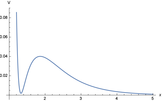
Figure 1: The effective potential (6) as a function of $x=T+T^{*}$ for $n=4,\lambda=-1,c_{n}=3$.

This is not the first example of stabilization of the real part of $T$ (see, for example, [21]), but stabilization of the imaginary part has proved more elusive (see, however, [27]). In particular, the effective potential (6) is independent of $y$. In order to explore how $y$ may also be stabilized, we next consider adding instead to the no-scale Kähler potential a dependence on the imaginary part of the modulus $T$ that is also of power-law form, though not sharing its motivation from calculations of $\alpha^{\prime}$ corrections in string theory [23, 24]:

$$K\;=\;-3\ln\left(T+T^{*}\right)+\frac{d_{m}}{|T-T^{*}|^{m}}\,.$$ (7)

In this case the effective potential takes the following form for $x,y>0$:

$$V = \frac{1}{x^{3}}\exp{\Big{[}d_{m}y^{-m}+\lambda x\Big{]}}\Big{[}-3+$$ (8)

$$\frac{1}{\left(-d_{m}m(m+1)y^{-m-2}+\frac{3}{x^{2}}\right)}\left(-d_{m}m\,y^{-m-1}+\lambda-\frac{3}{x}\right)\left(d_{m}m\,y^{-m-1}+\lambda\frac{3}{x}\right)\Big{]}\,.$$

Fig. 2 displays two slices through the effective potential (8) for $c_{n}=0,d_{m}=-0.05,m=3/2$ and $\lambda=-1$. In the left panel we show an $x$ slice for fixed $y=0.3$, and in the right panel we show a $y$ slice for fixed $x=0.3$. We see that in both slices there is a non-trivial minimum. We have also explored whether this example is suitable for inflation, but found that this was not the case, and so do not consider further the $c_{n}=0$ option.

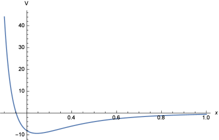
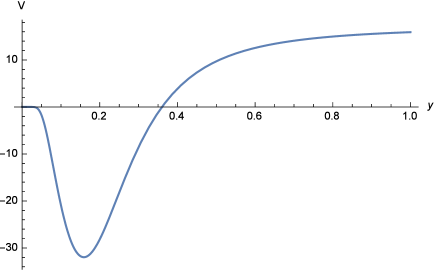
Figure 2: The effective potential obtained from (7) for $d_{m}=-0.05,m=3/2,\lambda=-1$ is plotted in the left panel as a function of $x$ for fixed $y=0.3$, and in the right panel as a function of $y$ for fixed $x=0.3$.

We have instead considered adding both the $T+T^{*}$-dependent term in (4) and the $T-T^{*}$-dependent term in (7) simultaneously to the no-scale Kähler potential:

$$K\;=\;-3\ln\left(T+T^{*}\right)+\frac{c_{n}}{|T+T^{*}|^{n}}+\frac{d_{m}}{|T-T^{*}|^{m}}\,.$$ (9)

In this case the effective potential takes the following form for $x,y>0$:

$$V = \frac{1}{x^{3}}\exp{\Big{[}c_{n}x^{-n}+d_{m}y^{-m}+\lambda x\Big{]}}\Big{[}-3+$$ (10)

$$\frac{1}{{c_{n}n(n+1)x^{-n-2}-d_{m}m(m+1)y^{-m-2}+\frac{3}{x^{2}}}}\left(-c_{n}n\,x^{-n-1}-d_{m}m\,y^{-m-1}+\lambda-\frac{3}{x}\right)\times$$

$$\times\left(-c_{n}n\,x^{-n-1}+d_{m}m\,y^{-m-1}+\lambda\frac{3}{x}\right)\Big{]}\,.$$

Fig. 3 shows slices through the effective potential (10) for the choices $n=-2,m=3/2,\lambda=-1,c_{n}=-5.9,d_{m}=-4.44$. The upper panel shows the $x$ dependence of the potential for several fixed values of $y$ and the lower panel shows the $y$ dependence for several fixed values of $x$. We see that the real component $x$ of the modulus $T$ is fixed at a non-zero value for the values $y=\{0.5,0.7\}$, and that the imaginary component $y$ is fixed at a non-zero value for the values $x=\{0.04,0.06,0.08,0.1\}$.

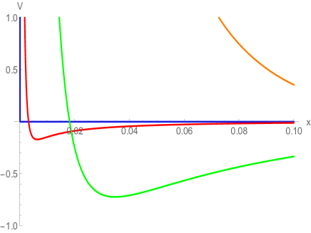
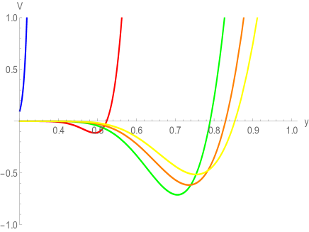
Figure 3: The effective potential (10) for $n=-2,m=3/2,\lambda=-1,c_{n}=-5.9,d_{m}=-4.44$ is plotted in the upper panel as a function of $x$, with the blue, red, green, and orange lines corresponding to $y=\{0.3,0.5,0.7,0.9\}$, and in the lower panel as a function of $y$ with the blue, red, green, orange and yellow lines corresponding to $x=\{6\,10^{-6},0.004,0.04,0.06,0.08,0.1\}$.

Fig. 4 shows a 3-dimensional image of the potential (10) for the same parameter choices $n=-2,m=3/2,\lambda=-1,c_{n}=-5.9,d_{m}=-4.44$ used in Fig. 3. This confirms that there is indeed a global minimum of the potential with $x,y\neq 0$. Thus, the Ansatz (9) achieves the goal of fixing both the components of the modulus field $T$.

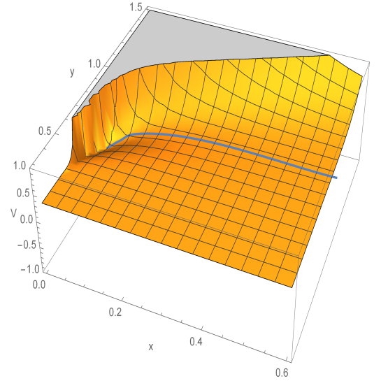
Figure 4: The effective potential (10) is plotted as a function of $x$ and $y$ for $n=-2,m=3/2,\lambda=-1,c_{n}=-5.9,d_{m}=-4.44$. A global minimum with $x,y\neq 0$ is clearly present. Also shown as a blue line is a possible field trajectory.

3 A Realization of Inflation

The effective potential shown in Fig.(4) exhibits an extended flat region in addition to the global minimum, and we now study whether there are field trajectories ending in the minimum that are suitable for cosmological inflation. In order to check this, we need to solve the equations of motion for the modulus field components $x,y$ in an expanding Universe described by a Friedman-Robertson-Walker (FRW) metric

$$ds^{2}=-dt^{2}+a(t)^{2}d\overrightarrow{x}^{2}\,,$$ (11)

corresponding to the action

$$S=\int\sqrt{-g}[K_{TT^{*}}\partial_{\mu}T\partial^{\mu}T^{*}-V]d^{4}x\,.$$ (12)

in curved space. Assuming a homogeneous FRW background, only the time derivative survives in the kinetic term and we obtain the following effective Lagrangian

$$L = a(t)^{3}[K_{TT^{*}}(x,y)(\dot{x}^{2}+\dot{y}^{2})-V(x,y)]\,,$$ (13)

where

$$K_{TT^{*}} = \left(c_{n}n(n+1)x^{-n-2}-d_{m}m(m+1)y^{-m-2}+e_{p}p(p+1)x^{-p-2}+\frac{3}{x^{2}}\right)\,.$$

Combining with Einstein’s equations for the scale factor $a(t)$, we get the following system of differential equations that describe completely the field evolution:

$$\frac{d}{dt}\left(\frac{\partial L}{\partial\dot{x}}\right)-\frac{\partial L}{\partial x} = 0\,,$$ (14)

$$\frac{d}{dt}\left(\frac{\partial L}{\partial\dot{y}}\right)-\frac{\partial L}{\partial y} = 0\,,$$ (15)

$$H^{2} = \frac{1}{3}\Big{[}K_{TT^{*}}(x,y)(\dot{x}^{2}+\dot{y}^{2})+V(x,y))\Big{]}\,.$$ (16)

A representative solution of these equations of motions is also shown in Fig. 4, as a blue line that starts at $\{x,y\}=\{0.7,1\}$ and terminates at the global minimum.

Fig. 5 displays the evolutions along the field trajectory shown in Fig. 4 of the real and imaginary components $\{x,y\}$ of $T$ as functions of time, as red and yellow lines, respectively. We see that $x$ decreases smoothly for $t\lesssim 240$, after which its value evolves only slowly, exhibiting small oscillations. The value of $y$ changes by $\lesssim 10$% for $t\lesssim 240$, after which it drops to an almost constant value that also exhibits small oscillations.

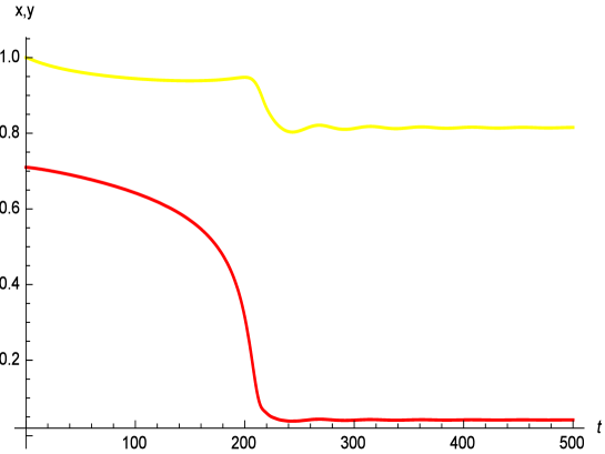
Figure 5: The field components $x$ and $y$ are plotted in red and yellow, respectively, as functions of the time $t$ along the field trajectory shown in Fig. 4.

Integrating the background equations we can compute the slow-roll parameters along the field trajectories, where we adopt the following definitions [28]:

$$\epsilon_{1} = -\dot{H}/H^{2}\,,$$ (17)

$$\epsilon_{i+1} \equiv \dot{\epsilon}_{i}/(H\epsilon_{i})\,,$$ (18)

$$n_{s}-1 = -2\epsilon_{1}-\epsilon_{2}-2\epsilon_{1}^{2}\,,$$ (19)

$$r = 16\epsilon_{1}\,.$$ (20)

Fig. 6 displays the evolutions along the field trajectory shown in Fig. 4 of the Hubble parameter $H$ (green line), the slow-roll parameter $\epsilon_{1}$ (blue line), and the number of e-folds of expansion $N$ (black line, rescaled by a reference value of 70). We see that the Hubble parameter varies only slowly until a time $t\simeq 200$, falling to much smaller values when $t\gtrsim 240$. Correspondingly, the number of e-folds $N$ increases nearly linearly until $t\sim 200$, after which it is nearly constant. The value of $\epsilon$ is small until a similar value of $t$, after which it enters a period of damped oscillations with amplitudes that are initially ${\cal O}(1)$.

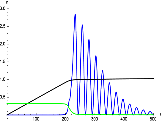
Figure 6: The Hubble parameter $H$, the slow-roll parameter $\epsilon$ and the rescaled number of e-folds $N/70$ are plotted as functions of time along the field trajectory shown in Fig. 4 as green, blue and black lines, respectively.

The initial conditions $x_{i}=0.71,y_{i}=1,\dot{y_{i}}=\dot{x_{i}}=0$ lead to the field trajectory shown in Fig. 4, which yields a number of e-folds $N\sim 55$, a scalar perturbation tilt $n_{s}=0.967$ and tensor-to-scalar perturbation ratio $r=0.00069$, which are compatible with the observational constraints [25]. Other choices of initial conditions also yield acceptable inflationary trajectories. For example, changing the initial value of $y$ to $0.9$ but keeping the initial value of $x$ fixed yields $n_{s}=0.961$ and $r=0.00030$, whilst $y=1.1$ yields $n_{s}=0.967$ and $r=0.00075$, also compatible with the observations. On the other hand, for initial values of $y<0.7$ the non-triviality of the kinetic terms requires a deeper analysis than the approximate treatment that is adequate for larger values of $y$.

4 Conclusions

We have presented in this paper a simple scenario for fixing both components of the modulus $T$ in the minimal no-scale supergravity model with Kähler potential $K=-3\ln(T+T^{\dagger})$, which is partly based upon calculations of theoretical calculations of corrections to this structure [23, 24]. In addition to yielding an effective potential that possesses a well-defined, unique minimum, this simple model exhibits a plateau at larger values of the components of $T$. We have found examples of field trajectories starting from initial values in this plateau region that yield an acceptable number of e-folds of inflation and values of the CMB observables $n_{s}$ and $r$ that are compatible with observation [25].

One interesting direction for future research will be to map out more completely the parameter space of initial field values that are compatible with cosmological observations, another will be to reconcile it better with string considerations, and another will be to integrate this simple scenario into a framework with matter particles and a scenario for reheating that would enable the number of inflationary e-folds to be calculated. In this way, the simple model presented in this paper may serve as the kernel of a more complete cosmological model.

References

- [1] A. A. Starobinsky, Phys. Lett. B 91, 99 (1980).
- [2] A. H. Guth, Phys. Rev. D 23 (1981) 347 doi:10.1103/PhysRevD.23.347.
- [3] V. F. Mukhanov and G. V. Chibisov, JETP Lett. 33, 532 (1981) [Pisma Zh. Eksp. Teor. Fiz. 33, 549 (1981)].
- [4] A. D. Linde, Phys. Lett. 108B (1982) 389 doi:10.1016/0370-2693(82)91219-9; A. Albrecht and P. J. Steinhardt, Phys. Rev. Lett. 48 (1982) 1220 doi:10.1103/PhysRevLett.48.1220.
- [5] See, for example JCAP 0310 (2003) 013 doi:10.1088/1475-7516/2003/10/013 [hep-th/0308055].
- [6] L. Maiani, Proc. Summer School on Particle Physics, Gif-sur-Yvette, 1979 (IN2P3, Paris, 1980) p. 3; G. ’t Hooft, in: G. ’t Hooft et al., eds., Recent Developments in Field Theories (Plenum Press, New York, 1980); E. Witten, Nucl. Phys. B188 (1981) 513; R.K. Kaul, Phys. Lett. 109B (1982) 19; J. R. Ellis, J. S. Hagelin, D. V. Nanopoulos, K. A. Olive and M. Srednicki, Nucl. Phys. B 238 (1984) 453 doi:10.1016/0550-3213(84)90461-9; J. Ellis, S. Kelley and D.V. Nanopoulos, Phys. Lett. B260 (1991) 131; U. Amaldi, W. de Boer and H. Furstenau, Phys. Lett. B260 (1991) 447; P. Langacker and M. Luo, Phys. Review D44 (1991) 817; C. Giunti, C. W. Kim and U. W. Lee, Mod. Phys. Lett. A 6 (1991) 1745; J. R. Ellis, G. Ridolfi and F. Zwirner, Phys. Lett. B 257 (1991) 83; H. E. Haber and R. Hempfling, Phys. Rev. Lett. 66 (1991) 1815; Y. Okada, M. Yamaguchi and T. Yanagida, Prog. Theor. Phys. 85 (1991) 1.
- [7] J. R. Ellis, D. V. Nanopoulos, K. A. Olive and K. Tamvakis, Phys. Lett. 118B (1982) 335; J. R. Ellis, D. V. Nanopoulos, K. A. Olive and K. Tamvakis, Nucl. Phys. B 221 (1983) 52; K. Nakayama and F. Takahashi, JCAP 1110, 033 (2011) [arXiv:1108.0070 [hep-ph]].
- [8] D. V. Nanopoulos, K. A. Olive, M. Srednicki and K. Tamvakis, Phys. Lett. B 123, 41 (1983); R. Holman, P. Ramond and G. G. Ross, Phys. Lett. B 137, 343 (1984); A. B. Goncharov and A. D. Linde, Phys. Lett. B 139, 27 (1984).
- [9] E. Cremmer, S. Ferrara, C. Kounnas and D. V. Nanopoulos, Phys. Lett. B 133 (1983) 61; J. R. Ellis, A. B. Lahanas, D. V. Nanopoulos and K. Tamvakis, Phys. Lett. B 134 (1984) 429.
- [10] J. R. Ellis, C. Kounnas and D. V. Nanopoulos, Nucl. Phys. B 241, 406 (1984).
- [11] J. R. Ellis, C. Kounnas and D. V. Nanopoulos, Nucl. Phys. B 247 (1984) 373.
- [12] A. B. Lahanas and D. V. Nanopoulos, Phys. Rept. 145 (1987) 1.
- [13] A. S. Goncharov and A. D. Linde, Class. Quant. Grav. 1, L75 (1984).
- [14] C. Kounnas and M. Quiros, Phys. Lett. B 151, 189 (1985).
- [15] J. R. Ellis, K. Enqvist, D. V. Nanopoulos, K. A. Olive and M. Srednicki, Phys. Lett. 152B (1985) 175 Erratum: [Phys. Lett. 156B (1985) 452].
- [16] K. Enqvist, D. V. Nanopoulos and M. Quiros, Phys. Lett. B 159, 249 (1985); P. Binétruy and M. K. Gaillard, Phys. Rev. D 34, 3069 (1986); H. Murayama, H. Suzuki, T. Yanagida and J. Yokoyama, Phys. Rev. D 50, 2356 (1994) [arXiv:hep-ph/9311326]; S. C. Davis and M. Postma, JCAP 0803, 015 (2008) [arXiv:0801.4696 [hep-ph]]; S. Antusch, M. Bastero-Gil, K. Dutta, S. F. King and P. M. Kostka, JCAP 0901, 040 (2009) [arXiv:0808.2425 [hep-ph]]; S. Antusch, M. Bastero-Gil, K. Dutta, S. F. King and P. M. Kostka, Phys. Lett. B 679, 428 (2009) [arXiv:0905.0905 [hep-th]]; R. Kallosh and A. Linde, JCAP 1011, 011 (2010) [arXiv:1008.3375 [hep-th]]; R. Kallosh, A. Linde and T. Rube, Phys. Rev. D 83, 043507 (2011) [arXiv:1011.5945 [hep-th]]; S. Antusch, K. Dutta, J. Erdmenger and S. Halter, JHEP 1104 (2011) 065 [arXiv:1102.0093 [hep-th]]; R. Kallosh, A. Linde, K. A. Olive and T. Rube, Phys. Rev. D 84, 083519 (2011) [arXiv:1106.6025 [hep-th]]; T. Li, Z. Li and D. V. Nanopoulos, JCAP 1402, 028 (2014) [arXiv:1311.6770 [hep-ph]]; W. Buchmuller, C. Wieck and M. W. Winkler, Phys. Lett. B 736, 237 (2014) [arXiv:1404.2275 [hep-th]].
- [17] J. Ellis, D. V. Nanopoulos and K. A. Olive, Phys. Rev. Lett. 111 (2013) 111301 [arXiv:1305.1247 [hep-th]].
- [18] J. Ellis, M. A. G. Garcia, D. V. Nanopoulos and K. A. Olive, Class. Quant. Grav. 33 (2016) no.9, 094001 doi:10.1088/0264-9381/33/9/094001 [arXiv:1507.02308 [hep-ph]].
- [19] E. Witten, Phys. Lett. 155B (1985) 151 doi:10.1016/0370-2693(85)90976-1.
- [20] S. Kachru, R. Kallosh, A. D. Linde and S. P. Trivedi, Phys. Rev. D 68 (2003) 046005 doi:10.1103/PhysRevD.68.046005 [hep-th/0301240].
- [21] J. R. Ellis, C. Kounnas and D. V. Nanopoulos, Phys. Lett. 143B (1984) 410 doi:10.1016/0370-2693(84)91492-8; J. Ellis, D. V. Nanopoulos and K. A. Olive, JCAP 1310 (2013) 009 doi:10.1088/1475-7516/2013/10/009 [arXiv:1307.3537 [hep-th]].
- [22] D. J. E. Marsh, Phys. Rept. 643 (2016) 1 doi:10.1016/j.physrep.2016.06.005 [arXiv:1510.07633 [astro-ph.CO]].
- [23] L. J. Dixon, V. Kaplunovsky and J. Louis, Nucl. Phys. B 329 (1990) 27 doi:10.1016/0550-3213(90)90057-K.
- [24] K. Becker, M. Becker, M. Haack and J. Louis, JHEP 0206 (2002) 060 doi:10.1088/1126-6708/2002/06/060 [hep-th/0204254]; R. Minasian, T. G. Pugh and R. Savelli, JHEP 1510 (2015) 050 doi:10.1007/JHEP10(2015)050 [arXiv:1506.06756 [hep-th]].
- [25] P. A. R. Ade et al. [Planck Collaboration], Astron. Astrophys. 594, A13 (2016) [arXiv:1502.01589 [astro-ph.CO]]. P. A. R. Ade et al. [Planck Collaboration], Astron. Astrophys. 594, A20 (2016) [arXiv:1502.02114 [astro-ph.CO]].
- [26] E. Cremmer, B. Julia, J. Scherk, S. Ferrara, L. Girardello and P. van Nieuwenhuizen, Nucl. Phys. B 147, 105 (1979); E. Cremmer, S. Ferrara, L. Girardello and A. Van Proeyen, Nucl. Phys. B 212, 413 (1983) doi:10.1016/0550-3213(83)90679-X.
- [27] J. Ellis, M. A. G. Garcia, D. V. Nanopoulos and K. A. Olive, JCAP 1408 (2014) 044 doi:10.1088/1475-7516/2014/08/044 [arXiv:1405.0271 [hep-ph]].
- [28] See, for example, D. H. Lyth and A. R. Liddle, The primordial density perturbation: Cosmology, inflation and the origin of structure, Cambridge, UK: Cambridge Univ. Pr. (2009).