Minimum Energy Paths and Transition States by Curve Optimization

Abstract

Transition states and minimum energy paths are essential to understand and predict chemical reactivity. Double-ended methods represent a standard approach for their determination. We introduce a new double-ended method that optimizes reaction paths described by curves. Unlike other methods, our approach optimizes the curve parameters rather than distinct structures along the path. With molecular paths represented as continuous curves, the optimization can benefit from the advantages of an integral-based formulation. We call this approach ReaDuct and demonstrate its applicability for molecular paths parametrized by B-spline curves.

I Introduction

To describe, understand, and design chemical reactivity, a multitude of different possible reactants and intermediates and a myriad of ways in which they can interact must be elucidated. ross2008a ; ludlow2008a ; bell2011a ; masters2011a ; vinu2012a ; simm2017a A key concept for this endeavor are elementary reactions that connect two reaction valleys.

To extract kinetic information of an elementary reaction, it is often sufficient to consider only one that leads to the smallest energy barrier. The point with the highest energy along such a path is the transition state (TS). It is a first-order saddle point on the potential energy surface (PES), for which the matrix of second partial derivatives of the electronic energy with respect to the nuclear coordinates (the Hessian) has exactly one negative eigenvalue. If one follows the mode corresponding to the negative Hessian eigenvalue in both directions along the steepest descent direction, one approaches two valleys of stable structures, and the path so generated is called a minimum energy path (MEP). All along a MEP, the path tangent is parallel to the nuclear gradient of the electronic energy. There may exist multiple transition states connecting two molecular structures, and, accordingly, for each one we will have a different MEP.

Many algorithms to optimize transition states fall into the category of double-ended methods. elber1987a ; ayala1997a ; peng1993a ; jonsson1998a ; henkelman2000a ; henkelman2000b ; trygubenko2004a ; weinan2002a ; weinan2005a ; burger2006a ; burger2007a ; chaffeymillar2012a ; peters2004a ; goodrow2008a ; behn2011a ; sharada2012a ; granot2008a ; ghasemi2011a ; plessow2013a ; sheppard2008a ; zimmerman2013b These methods aim to determine a path connecting reactant and product valleys through the transition state structure. Some of the double-ended methods gradually construct the path starting from both ends until they connect, while others start from a reaction path guess and optimize it. Examples belonging to the former category are the growing string methodpeters2004a and the freezing string method,behn2011a ; sharada2012a whereas the nudged elastic band (NEB) methodjonsson1998a ; henkelman2000a ; henkelman2000b and the string methodweinan2002a ; weinan2005a are examples of the latter category. The NEB method approximates the reaction path by a series of distinct structures (called beads or images) and optimizes them until they represent a good estimate of the minimum energy path. To achieve this, each image undergoes a force made up of a spring force to ensure that all images are evenly spaced, and of a force perpendicular to the path that is projected from the quantum chemical forces acting on the atomic nuclei. The string method describes the reaction path as a curve, which is updated iteratively. At each step, structures are selected along the path, undergo a steepest descent iteration step, after which the curve is reparametrized to fit the new finite set of structures.

The reaction path delivered by double-ended methods is an approximation for the minimum energy path. Accordingly, the structure along this reaction path with the highest electronic energy can be taken as an approximate transition state. The exact transition state may then be optimized until the Hessian has exactly one negative eigenvalue. For this optimization, one may rely on eigenvector following methods.cerjan1981a ; simons1983a ; baker1986a ; jensen1995a ; bergeler2015b In a recent work,zimmerman2013b exact transition state search was integrated in the double-ended optimization formalism to obtain the exact transition state directly during a reaction path optimization.

The new algorithm ReaDuct presented in this work optimizes reaction paths described by (continuous) curves. Unlike the NEB and string methods, however, it does not update iteratively structures along the path, but directly the curve itself as a whole (or, more precisely, its parametrization). This ensures that the reaction path description is truly continuous rather than discrete, and allows for an optimization formalism relying on integrals along reaction paths. Accordingly, the mathematical nature of the optimization is independent of the specific discretization and the optimization result can be improved at will by refining the integration grid.

ReaDuct is related to the splined saddle method,granot2008a ; ghasemi2011a which also relies on a parametrized curve and a minimization scheme for finding the transition state. In the splined saddle method, however, the main goal of the optimization procedure is the transition state itself and the MEP is generated in a second step, while ReaDuct directly optimizes the full path between reactants and products.

We first introduce a general formalism for the optimization of curves in Section II. Then, in Section III, we detail the application of this formalism for the optimization of reaction paths. We describe our implementation of ReaDuct in Section IV and study its application on various examples in Section V.

II Formalism: Curve optimization

In this section we discuss two formalisms for optimizing curves with regard to some optimization target. The term optimization target designs a general goal that drives the optimization of the curve. The optimization of reaction paths will build on this formalism and will be discussed in the next section.

We consider a curve $\bm{\mathcal{C}}(u)\in\mathbb{R}^{n}$ in $n$ dimensions defined on the domain $u\in\left[u_{\mathrm{start}},u_{\mathrm{end}}\right]$, $u\in\mathbb{R}$ and parametrized by $K$ parameters $p_{i}$, $1\leq i\leq K$. We consider scalar parameters, but note that depending on the specific curve parametrization, it may be possible to unite such parameters to $n$-dimensional parameter vectors.

To obtain the set of parameters $\{p_{i}\}$ that best fit the optimization target, we consider formalisms that are force- and cost-based.

II.1 Force-based formalism

Given a curve, it is often straightforward to alter it in order to improve it with respect to some optimization target. In the force-based formalism, one applies artificial forces $\bm{f}_{\mathrm{local}}(u)\in\mathbb{R}^{n}$ along the curve such that their action improves the current curve. These artificial forces are propagated back to the curve parametrization and deliver forces $F_{\mathrm{local},i}(u)$ ($1\leq i\leq K$) acting on the curve parameters $p_{i}$. The full force on the curve parameters is then the sum of all contributions along the curve, $F_{i}=\int_{u_{\mathrm{start}}}^{u_{\mathrm{end}}}F_{\mathrm{local},i}(u)\mathop{}\!\mathrm{d}u$. How to propagate the forces back depends on the choice of parametrization. The curve parameters can then be updated iteratively with an optimization algorithm such as steepest descent, FIRE,bitzek2006a Verlet, etc. The force-based optimization formalism is illustrated in Fig. 1.

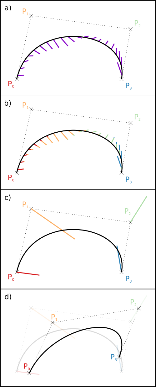
Figure 1: Force-based optimization step of a Bézier curve parametrized by four two-dimensional points. a) Forces, represented by purple lines, are applied along the curve. b) Each force can be split into contributions for the different parameters, represented by colors corresponding to the parameters. c) The force for each parameter point is obtained as the sum of its contributions along the path. d) The curve is updated by changing the parameters according to the force they experience.

II.2 Cost-based formalism

In a cost-based formalism, the optimization target is formulated as an objective function or cost $c$ that is to be minimized. A cost is assigned to every possible curve, and the cost can be expressed as a function of the curve parameters. To optimize the curve, one updates the curve parameters iteratively to decrease the cost of the curve. When the derivatives of the cost with respect to the curve parameters are available, efficient optimization schemes can be applied for this purpose. Examples of such schemes are the conjugate gradient method or the Broyden–Fletcher–Goldfarb–Shanno (BFGS) method.nocedal2006a

Depending on the optimization target, one may attribute a local cost for each point along the curve, expressed as a function $c_{\mathrm{local}}(u)$. The total cost is then obtained by integrating $c_{\mathrm{local}}$ along the curve,

$$c=\int_{u_{\mathrm{start}}}^{u_{\mathrm{end}}}c_{\mathrm{local}}(u)\mathop{}\!\mathrm{d}u.$$ (1)

Then, the problem may also be formulated in the force-based formalism by choosing

$$F_{\mathrm{local},i}(u)=-\frac{\partial c_{\mathrm{local}}(u)}{\partial p_{i}}.$$ (2)

II.3 General Comments

Both formalisms presented above are valid for any parametrizaton choice. The specific parametrization will define the flexibility of the curve, and therefore the ensemble of curves that can be realized. In general, more parameters will allow for more flexibility, and the obtained curves will fit the optimization target better.

It is important to understand that the curve is optimized as a whole by adjusting its curve parameters; one does not optimize single points along the curve. When integrating the force or the cost along the curve, this formalism allows for improving the optimization result without changing the nature of the problem by increasing the number of integration points.

III Reaction path optimization

Reaction paths for molecular systems of $N$ atoms can be represented as curves in $n=3N$ dimensions (here, we assume Cartisian coordinates; in principle, one can also work with internal coordinates). Both the force-based and cost-based formalisms for curve optimization can be applied to reaction paths if an adequate optimization target is formulated. The choice of a specific target may depend on the available computational resources, size of the molecular system, or desired accuracy of the optimized reaction path. Note that the formalism presented here can also be applied on molecular paths for other purposes than the optimization of reaction paths.

We do not consider a universal choice for the optimization target the best strategy, neither in the force-based nor in the cost-based formalism. Below, we therefore introduce two possible targets, that require only the electronic energy and its gradient, Note, however, that the formalism also supports optimization targets depending on higher derivatives of the electronic energy.

To select an adequate optimization target, it may help to consider a two-dimensional system and regard the energy as a third dimension. In this case, one can illustrate a reaction path by a pipe connecting two valleys separated by mountains. In this analogy, at any time during the optimization one knows the position of the pipe, its relative height (energy), and the inclination of the landscape (gradient) along the curve. From this information, one must decide how to alter the pipe to improve it (i.e., turn it more into a minimum energy path).

III.1 Force-based reaction path optimization

Given a reaction path, a reasonable direction to alter the path is downward in energy. Therefore, in the force-based formalism a natural choice for the forces to apply along the path is the perpendicular projection of the negative gradient of the electronic energy. For a minimal energy path, the gradient of the energy is parallel to the path and therefore no forces are applied.

To improve convergence, especially for flat parts of the potential energy surface, one can add a contribution for the path tension.

The force applied on the curve is therefore given by

$$\bm{f}_{\mathrm{local}}(u)=(1-\alpha_{\mathrm{f}})\cdot\bm{f}_{\mathrm{perp}}(u)+\alpha_{\mathrm{f}}\cdot\bm{f}_{\mathrm{para}}(u),$$ (3)

where $\alpha_{\mathrm{f}}$ is a parameter of the method (the subscript ‘f’ relates to the force-based formalism). The perpendicular contribution from the negative gradient of the electronic energy is given by

$$\bm{f}_{\mathrm{perp}}(u)=-\left(\bm{\nabla}E_{\mathrm{el}}(\bm{\mathcal{C}}(u))\right)_{\perp}\cdot\frac{r_{\mathrm{Bohr}}^{2}}{E_{\mathrm{h}}},$$ (4)

where $E_{\mathrm{h}}$ is the Hartree energy unit and $r_{\mathrm{Bohr}}$ is the Bohr radius, and the path tension contribution is parallel to the reaction path,

$$\bm{f}_{\mathrm{para}}(u)=2\cdot\left(\left(\bm{\mathcal{C}}^{\prime}(u)\right)^{T}\bm{\mathcal{C}}^{\prime\prime}(u)\right)\cdot\hat{\bm{t}}\cdot\frac{1}{r_{\mathrm{Bohr}}},$$ (5)

where $\hat{\bm{t}}$ denotes the unit tangent. Note that the forces defined here have the dimension of a length for practical reasons. Since these forces have no true physical meaning, other units would be possible. Note that this formulation is one of a multitude of possibilities. It is closely related to the NEB method and could be considered its continous-path equivalent.

III.2 Cost-based reaction path optimization

To optimize a reaction path in the cost-based formalism, one must reduce its information to a single number (its cost). This requires special care, since artefacts may arise depending on the cost formulation.

To illustrate this issue, let us consider a cost function $c_{1}$ equal to the integral of the energy along the reaction path. Note that similar strategies were followed based on a discretized reaction path.elber1987a ; ayala1997a This cost can be formulated as

$$c_{1}=\int_{u_{\mathrm{start}}}^{u_{\mathrm{end}}}E_{\mathrm{el}}(\bm{\mathcal{C}}(u))\mathop{}\!\mathrm{d}L,$$ (6)

where

$$\mathop{}\!\mathrm{d}L=\left\lVert\frac{\partial\bm{\mathcal{C}}(u)}{\partial u}\right\rVert\mathop{}\!\mathrm{d}u=\left\lVert\bm{\mathcal{C}}^{\prime}(u)\right\rVert\mathop{}\!\mathrm{d}u$$ (7)

is an infinitesimal path segment. While $c_{1}$ may be reasonable, it is based on a multiplication of a length with an energy. Hence, not only $c_{1}$, but also the position of the optimized curve depends on the energy reference. Furthermore, minimization of $c_{1}$ will fail for negative energies, because in such a case the cost keeps decreasing for increasing reaction path lengths.

To remove the dependence on the energy reference, one can normalize the cost by dividing it by the total path length,

$$c_{2}=\frac{c_{1}}{\displaystyle\int_{u_{\mathrm{start}}}^{u_{\mathrm{end}}}\mathop{}\!\mathrm{d}L}.$$ (8)

$c_{2}$ will still depend on the energy reference, but the position of its minima will not. However, another artefact is introduced: for a given reaction path, the cost can be lowered if the path length increases in low-energy regions and thereby reduces the weight of high-energy regions.

To avoid these issues for $c_{1}$ and $c_{2}$, one may define the related cost function

$$c_{3}=\int_{u_{\mathrm{start}}}^{u_{\mathrm{end}}}E_{\mathrm{el}}(\bm{\mathcal{C}}(u))\mathop{}\!\mathrm{d}u.$$ (9)

This formulation avoids the need for explicit normalization if the integration interval ($\left[u_{\mathrm{start}},u_{\mathrm{end}}\right]$) is constant. It may, however, lead to an uneven distribution of $u$ along the curve to increase the contribution of low-energy regions. To resolve this, one can add, similarly to the force-based reaction path optimization, a term for the curve tension:

$$c_{\mathrm{ReaDuct}}=(1-\alpha_{\mathrm{c}})\cdot c_{\mathrm{energy}}+\alpha_{\mathrm{c}}\cdot c_{\mathrm{tension}}$$ (10)

with

$$c_{\mathrm{energy}}=c_{3}\cdot\frac{1}{E_{\mathrm{h}}}=\left(\int_{u_{\mathrm{start}}}^{u_{\mathrm{end}}}E_{\mathrm{el}}(\bm{\mathcal{C}}(u))\mathop{}\!\mathrm{d}u\right)\cdot\frac{1}{E_{\mathrm{h}}}$$ (11)

and

$$c_{\mathrm{tension}}=\int_{u_{\mathrm{start}}}^{u_{\mathrm{end}}}\left(\frac{\partial\left\lVert\bm{\mathcal{C}}^{\prime}(u)\right\rVert^{2}}{\partial u}\right)^{2}\mathop{}\!\mathrm{d}u\cdot\frac{1}{r_{\mathrm{Bohr}}^{4}},$$ (12)

where $\alpha_{\mathrm{c}}$ is a parameter of the method (the $\mathrm{c}$ subscript relates to the cost-based formalism). Note that we define $c_{\mathrm{ReaDuct}}$ to have no units. In the following sections, all examples for the cost-based formalism will rely on $c_{\mathrm{ReaDuct}}$. Note that although the gradients of the electronic energy do not appear in $c_{\mathrm{ReaDuct}}$, they will be required for the reaction path optimization (through the derivatives of $c_{\mathrm{ReaDuct}}$ with respect to the curve parameters).

III.3 Initial reaction path

The reaction path from which the optimization is started is crucial for the course of the reaction path optimization. Especially, for reactions with multiple possible minimum energy paths, the choice of the initial reaction path will affect which one is obtained after optimization. While this is not the focus of the present work, we will mention a few common choices for initial paths.

Given some structures for the reactants and products of a reaction, one can generate an initial curve by interpolating between them. Note that the order of the atoms in the structure description must be identical in both structures (atom matching).

Another possibility to determine the initial reaction path is to fit a curve to a sequence of structures. This allows for processing reactivity information of first-principles molecular dynamics simulations, interactive explorations of reactivity, or PES scans (see the discussion in Ref. 35).

It is also possible to start from paths already available as curves, which can happen when starting from pre-processed reaction paths (see below) or from paths optimized with other quantum chemical methods.

Rotation and translation should be removed from the initial path, especially when the optimization target formulation depends on the curve tangent. Otherwise, the cost or forces underlying the reaction path optimization may depend on the overall rotation and translation of the molecular system. Removal of rotation and translation can for instance be achieved with the help of quaternions.coutsias2004a A formulation of the curve in internal coordinates avoids such issues.

III.4 Improved initial reaction path

The initial reaction path may be very different from the minimal energy path. This is often the case when the initial reaction path is generated by interpolation between start and end structures. In this case, it may be useful to improve this guess in order to reduce the number of single-point calculations required for the reaction path optimization, especially if this is possible without much computational effort (e.g., without explicit single-point calculations).

In our formalism, improvement can be achieved naturally by optimizing the path with a cost function $c_{\mathrm{improved}}$ that is independent of the electronic structure. One possibility is related to the image-dependent pair potential (IDPP) for initial paths in the NEB method.smidstrup2014a IDPP defines, for each image along the NEB path, a target distance for all pairs of atomic nuclei and an objective function that aims to match the target distances as closely as possible. We proceed similarly but define such an objective function along the (continuous) reaction path. The minimization of this cost function is naturally supported by the formalism detailed in the previous section. Hence, we define the cost for an improved initial reaction path as the integral along the path of the sum of pair potentials for the atomic nuclei,

$$c_{\mathrm{improved}}=\int_{u_{\mathrm{start}}}^{u_{\mathrm{end}}}\sum_{i}^{N}\sum_{j>i}^{N}V\left(r_{ij}(u),r_{\mathrm{target},ij}(u)\right)\mathop{}\!\mathrm{d}u,$$ (13)

where $r_{ij}(u)$ is the distance between atomic nuclei $i$ and $j$ at the curve coordinate $u$. It can be extracted from $\bm{\mathcal{C}}(u)$. $r_{\mathrm{target},ij}(u)$ is the target distance for this atom pair at $u$ and can be defined on the domain $\left[u_{\mathrm{start}},u_{\mathrm{end}}\right]$ as a linear interpolation between the internuclear distance at the start and end points of the reaction path,

$$r_{\mathrm{target},ij}(u)=\frac{u\cdot r_{ij}(u_{\mathrm{end}})+(u_{\mathrm{end}}-u)\cdot r_{ij}(u_{\mathrm{start}})}{u_{\mathrm{end}}-u_{\mathrm{start}}}.$$ (14)

Different choices can be adopted for the pair potential $V(r,r_{\mathrm{target}})$. For instance, the IDPP pair potential may be formulated as

$$V_{\mathrm{IDPP}}(r,r_{\mathrm{target}})=\frac{1}{r_{\mathrm{target}}^{4}}\left(r_{\mathrm{target}}-r\right)^{2}\cdot r_{\mathrm{Bohr}}^{2}.$$ (15)

IV Implementation

We implemented the ReaDuct algorithm as a module of our software package SCINE.scine SCINE provides implementations of the Parametrized Method 6 (PM6),stewart2007 the non-self-consistent density-functional tight-binding (DFTB) method,porezag1995 ; seifert1996 as well as DFTB2elstner1998 and DFTB3.gaus2011 These semiempirical methods enable reaction path optimization of molecular systems of moderate size in a few seconds. SCINE also offers the possibility to steer the quantum chemical programs ORCA,neese2012a Gaussiangaussian16 and Q-Chemshao2015a so that more advanced electronic structure methods are also available

We represent reaction paths as cubic B-spline curves. B-spline curves are functions $\bm{\mathcal{C}}(u)$ composed of $n$ piecewise polynomial segments of degree $p$, whereby $1\leq p\leq n$. A B-spline curve is given by

$$\bm{\mathcal{C}}(u)=\sum_{i=0}^{n}\mathcal{N}_{i,p}^{\bm{U}}(u)\,\bm{P}_{i},$$ (16)

where $\mathcal{N}_{i,p}^{\bm{U}}(u)$ are B-spline functions defined on a so-called knot vector $\bm{U}$. $\bm{P}_{i}$ is called control point vector. B-Spline curves are commonly defined on the interval $u\in\left[0,1\right]$. A detailed discussion can be found elsewhere.piegl1997a ; heuer2018a

The B-spline parameters subject to optimization are the coordinates of the control points. It is important to note that although the control points have the same dimension as structures along the curve, they should not be interpreted as such. In general, we do not optimize the first and last control points, which correspond to the two end points of the path.

In Appendix A, we illustrate how the derivatives of a cost function with respect to the control point coordinates can be calculated.

The applicability of ReaDuct is not limited to specific methods, and is applicable as long as energies and gradients are available. Apart from quantum chemical methods, molecular mechanics approaches can also be applied.

During reaction path optimization, the single-point calculations are accelerated with adequate initial electronic densities to reduce the number of self-consistent field iterations. This is currently achieved by storing the electronic density from one step to the next for each integration point along the path, but propagation approachesatsumi2008 ; atsumi2010 ; muehlbach2016a are also possible. Non-linear optimization of the curve cost relies on algorithms implemented in the dlib library.king2009a

SCINE is available in a graphical (window-based) and in a non-graphical variant. The graphical version allows for reaction path optimizations in real time and is especially adequate in combination with semiempirical methods. It shows the evolution of energy profiles during the optimization (Fig. 2) and the built-in molecular viewer illustrates the reaction path reaction coordinate (Fig. 3).

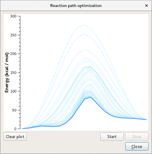
Figure 2: Window shown during a reaction path optimization. Every energy profile represents a reaction path visited during the optimization. The energy profile represented by the thickest line represents the current (most recent) reaction path.

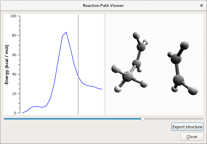
Figure 3: Window shown to visualize a reaction profile. A slider bar allows one to follow the reaction coordinate and show the corresponding molecular structures.

The non-graphical version is designed to be executed on the command line, possibly on high-performance-computing facilities. The non-graphical version of SCINE is more practical for automated reaction path optimizations such as those described in Refs. 52 and 6, large numbers of reaction path optimizations, or for more time-demanding single-point calculations. It reads in a YAMLyaml12 -formatted input file that describes the different tasks to performed. The input file can be generated interactively with the graphical program version. It is also possible to visualize the reaction paths calculated non-graphically in the graphical program version.

For analysis purposes of the obtained MEPs and transition states, SCINE also implements an eigenvector following methodbaker1986a and an intrinsic reaction coordinate following algorithm.

V Examples

To asses the reliability of the ReaDuct algorithm, we studied an example set of 20 reactions discussed in a related work about transition state optimization by Birkholz and Schlegel.birkholz2015a The interested reader can find a list of the reactions in Fig. 1 of Ref. 54. Below, the reaction labels will also refer to the ones defined in that figure of Ref. 54. Unless stated otherwise, the calculations refer to PM6 results.

In the Supporting Information, we discuss the choice and importance of the different ReaDuct parameters at the example set. There, we consider both force-based and cost-based formulations of ReaDuct, and show that cost-based optimizations require significantly fewer steps to obtain reasonable transition state candidates. Therefore, we focus on cost-based optimizations here.

The examples discussed below were all obtained with the same set of parameters. The optimized reaction paths were described by B-spline curves with five control points, and the integrations involved in the optimization considered 11 equidistant points along the reaction paths at uniformly distributed curve coordinates. A value of $10^{-5}$ was chosen for $\alpha_{\mathrm{c}}$, and the optimizations were stopped when the root mean square of the cost derivatives with respect to the curve parameters (control point coordinates) fell below $10^{-3}r_{\mathrm{Bohr}}^{-1}$. As can be seen in the Supporting Information, this threshold is adequate for a fast determination of transition state candidates. To improve on the transition state candidates, it is possible to choose a tighter threshold (but note that this will lead to a larger number of optimization steps and, accordingly, to an increased computational time). The BFGS optimization algorithm was used for the cost minimization. When applicable, the improved initial path was generated with the IDPP cost function in an optimization with 81 integration points, and a threshold for the root mean square of the cost derivatives of $10^{-5}r_{\mathrm{Bohr}}^{-1}$.

V.1 Application of ReaDuct from reactant and product structures

One can generate an initial reaction path by interpolating the coordinates given in the Supporting Information of Ref. 54. The results obtained with ReaDuct are shown in Table 1 for the cost-based formalism, with (IDPP, PM6) and without (PM6) improved initial path with the IDPP cost function.

For most cases, the transition state candidates delivered by ReaDuct are good approximations to the desired transition state. Exceptions are the Cope and OxyCope reactions, where other transition states with higher energies were found. In both cases, a better initial reaction path, such as the one discussed in the Supporting Information, leads to the correct transition state. The application of the IDPP cost function does not make a significant difference, except for cases in which the linear interpolation was particularly inadequate such as for the Cope, HCN, and OxyCope reactions.

Table 1: Results of the application of ReaDuct to the test reactions, starting from an interpolation between the structures for the reactants and products, in the cost-based formalism. $E_{\mathrm{ref}}$ refers to the energy of the transition state structure given in Ref. 54, in $E_{\mathrm{h}}$. $E_{\mathrm{ReaDuct}}$ is the energy of the transition state candidate delivered by ReaDuct in $E_{\mathrm{h}}$. $n_{\mathrm{it}}$ refers to the number of iteration steps in the optimization procedure, and can be multiplied by the number of integration points (here, 11) to determine the total number of single-point calculations.

		PM6		IDPP, PM6
Reaction	$E_{\mathrm{ref}}$	$n_{\mathrm{it}}$	$E_{\mathrm{ReaDuct}}$	$n_{\mathrm{it}}$	$E_{\mathrm{ReaDuct}}$
C2N2O	-34.7508	10	-34.7492	9	-34.7489
C5HT	-26.4037	19	-26.3938	28	-26.3935
Cope	-31.9092	208	-31.6953	86	-31.7216
CPHT	-25.3950	6	-25.3899	10	-25.3880
Cyc-But	-20.8842	10	-20.8772	29	-20.8796
DACP2	-50.8593	18	-50.8394	43	-50.8419
DACP+eth	-36.3806	8	-36.3713	12	-36.3720
DFCP	-50.0347	24	-50.0136	32	-50.0159
Ene	-27.3982	31	-27.3522	60	-27.3536
Grignard	-112.9261	32	-112.9016	35	-112.8954
H2+CO	-16.0850	18	-16.0831	21	-16.0833
HCN	-11.4217	477	-11.4146	17	-11.4202
HF+eth	-28.7245	14	-28.7170	27	-28.7178
Hydro	-66.8948	45	-66.8368	69	-66.8226
MeOH	-17.0795	30	-17.0437	43	-17.0436
Oxirane	-88.1479	17	-88.1376	31	-88.1442
OxyCope	-37.1128	361	-36.9411	105	-36.9472
Silane	-4.5768	18	-4.5583	22	-4.5583
SN2	-32.7061	10	-32.7032	13	-32.7035
Sulfolene	-48.7413	36	-48.7231	56	-48.7194

V.2 Application of ReaDuct from sequences of structures

To have more control over the specific local transition states, the initial path can be generated from a sequence of structures corresponding roughly to the MEP of interest. We generated a set of 20 initial paths for the test reactions by conducting the reactions interactivelyhaag2014b in the SCINE extension for real-time quantum chemistry. The corresponding sequences of structures are available in the Supporting Information. B-spline curves were fit to the so generated sequences of structures, and a geometry optimization made sure that the initial reaction paths started and ended at stable structures.

Table 2 summarizes the optimization results. In all cases, the desired transition state was found. Starting the optimization from an improved guess with the IDPP cost function is beneficial in all cases and reduces the number of optimization steps. This observation can be ascribed to the fact that IDPP-optimized paths correspond to smoother transitions from reactants to products that are closer to the MEPs.

Table 2: Results of the application of ReaDuct to the test reactions, starting from sequences of structures generated in a haptic exploration, in the cost-based formalism. $E_{\mathrm{ref}}$ refers to the energy of the transition state structure given in Ref. 54, in $E_{\mathrm{h}}$. $E_{\mathrm{ReaDuct}}$ is the energy of the transition state candidate delivered by ReaDuct in $E_{\mathrm{h}}$. $n_{\mathrm{it}}$ refers to the number of iteration steps in the optimization procedure.

		PM6		IDPP, PM6
Reaction	$E_{\mathrm{ref}}$	$n_{\mathrm{it}}$	$E_{\mathrm{ReaDuct}}$	$n_{\mathrm{it}}$	$E_{\mathrm{ReaDuct}}$
C2N2O	-34.7508	39	-34.7476	11	-34.7481
C5HT	-26.4037	61	-26.3897	29	-26.3899
Cope	-31.9092	119	-31.7977	95	-31.8031
CPHT	-25.3950	18	-25.3908	13	-25.3912
Cyc-But	-20.8842	46	-20.8787	35	-20.8796
DACP2	-50.8593	66	-50.8473	24	-50.8436
DACP+eth	-36.3806	39	-36.3710	18	-36.3691
DFCP	-50.0347	13	-50.0314	12	-50.0304
Ene	-27.3982	91	-27.3440	62	-27.3511
Grignard	-112.9261	108	-112.8926	27	-112.8986
H2+CO	-16.0850	46	-16.0844	21	-16.0603
HCN	-11.4217	24	-11.4216	12	-11.4212
HF+eth	-28.7245	51	-28.7198	25	-28.7195
Hydro	-66.8948	89	-66.8498	61	-66.8482
MeOH	-17.0795	33	-17.0719	23	-17.0668
Oxirane	-88.1479	89	-88.1421	32	-88.1454
OxyCope	-37.1128	91	-37.0599	71	-37.0682
Silane	-4.5768	19	-4.5759	11	-4.5761
SN2	-32.7061	20	-32.7030	10	-32.7042
Sulfolene	-48.7413	51	-48.7013	71	-48.7052

V.3 Density Functional Theory

The application of ReaDuct to the example set was studied for density funtional theory (DFT). For the DFT single-point calculations, SCINE steered the Gaussian program package.gaussian16 The coordinates for reactant, product, and reference transition state structures were taken from Ref. 54. Table 3 summarizes the B3LYP/6-31G(d,p) results. It is also possible to start DFT reaction path optimizations with initial paths obtained from path optimizations with PM6. We studied this for the example set, and the results are also given in Table 3.

Some of the optimizations failed due to inadequate initial reaction paths or nonconverging calculations. These cases are flagged in Table 3. In all cases, starting from the PM6-optimized path reduced considerably the number of optimization steps.

Table 3: Results of the application of ReaDuct to the test reactions with B3LYP/6-31G(d,p). $E_{\mathrm{ref}}$ refers to the energy of the transition state structure given in Ref. 54, in $E_{\mathrm{h}}$. $E_{\mathrm{ReaDuct}}$ is the energy of the transition state candidate delivered by ReaDuct in $E_{\mathrm{h}}$. $n_{\mathrm{it}}$ refers to the number of iteration steps in the optimization procedure. Comments: [a] Unsuccesful because of nuclear overlap in the linear interpolation. [b] Unsuccesful because of inadequate IDPP guess. [c] SCF Calculations not converging during optimization. [d] Results obtained with the Gaussian flag ”SCF=XQC”.

		DFT		IDPP, DFT		PM6, DFT		IDPP, PM6, DFT
Reaction	$E_{\mathrm{ref}}$	$n_{\mathrm{it}}$	$E_{\mathrm{ReaDuct}}$	$n_{\mathrm{it}}$	$E_{\mathrm{ReaDuct}}$	$n_{\mathrm{it}}$	$E_{\mathrm{ReaDuct}}$	$n_{\mathrm{it}}$	$E_{\mathrm{ReaDuct}}$
C2N2O	-263.2163	12	-263.2153	9	-263.2153	3	-263.2149	3	-263.2150
C5HT	-195.2614	15	-195.2561	21	-195.2560	3	-195.2542	5	-195.2546
Cope	-234.5720	44	-234.5118	73	-234.5129	14	-234.5070	17	-234.5087
CPHT	-194.0664	10	-194.0611	12	-194.0590	3	-194.0547	3	-194.0547
Cyc-But	-155.9262	12	-155.9181	41	-155.9246	6	-155.9188	5	-155.9198
DACP2	-388.1902	14	-388.1681	35	-388.1746	8	-388.1727	3	-388.1739
DACP+eth	-272.6725	13	-272.6642	17	-272.6652	4	-272.6632	4	-272.6662
DFCP	-316.2708	9	-316.2609	10	-316.2593	6	-316.2601	4	-316.2568
Ene	-196.4582	32	-196.4215	54	-196.3996	10	-196.4200	8	-196.4217
Grignard	-3580.1803	22	-3580.1423	40	-3580.1430	17	-3580.1437	9	-3580.1393
H2+CO	-114.3649	24	-114.3623	18	-114.2560	8	-114.3597	9	-114.3560
HCN	-93.3474	Fail[a]	Fail[a]	Fail[b]	Fail[b]	10	-93.3360	9	-93.3356
HF+eth	-178.9610	19	-178.9582	32	-178.9588	10	-178.9577	9	-178.9569
Hydro	-460.5243	39	-460.4599	92	-460.4647	24	-460.4661	19	-460.4610
MeOH	-115.5732	21	-115.5442	42	-115.5457	9	-115.5316	10	-115.5327
Oxirane	-652.6848	26	-652.6675	40	-652.6712	8	-652.6651	9	-652.6711
OxyCope	-270.4669	Fail[a]	Fail[a]	Fail[c]	Fail[c]	22	-270.2363	25	-270.0815
Silane	-291.7942	32	-291.7674	51	-291.7656	25[d]	-291.7638[d]	28[d]	-291.7640[d]
SN2	-717.9007	14	-717.8972	27	-717.8978	11	-717.8991	6	-717.8992
Sulfolene	-704.5600	16	-704.5416	36	-704.5465	11	-704.5495	11	-704.5468

V.4 Video examples

Videos illustrating the real-time optimization of reaction paths can be found on the Internet.reaductVideos They illustrate the following:

• Cost-based optimization of the DACP+eth reaction (Diels–Alder reaction of cyclopentadiene and ethylene), followed by eigenvector following and normal mode analysis.

• Effect of the number of integration points for the optimization of the Grignard reaction (addition of phenyl magnesium bromide to benzophenone).

• Occurrence and cure of incorrect SCF convergencevaucher2017a during reaction path optimizations at the example of the Silane reaction (addition of silylene to H₂).

• How to find different transition states for the Cope reaction (Cope rearrangement of 1,4-hexadiene) by optimizing paths recorded in interactive explorations of chemical reactivity.

VI Conclusion and Outlook

In this work, we introduced the ReaDuct algorithm for the optimization of reaction paths and the search of transition states. ReaDuct is a double-ended method that relies on the optimization of curves rather than single structures along a path. This is achieved by updating the curve parameters directly.

We presented two formalisms to carry out an iterative optimization of a reaction path. Both aim at finding the curve that delivers the best fit to some given optimization target. In the force-based formalism, one defines artificial forces along the curve at every iteration step. These forces are propagated back to the curve parameters, which are then updated to alter the curve. In the cost-based formalism, the goal is to optimize the curve with respect to an objective function, or cost, expressed as a function of the curve parameters. The cost can be minimized by application of standard minimization algorithms.

For both formalisms, in the most common scenario the objective function can be defined locally for each point along the curve. Then, the optimization problem involves an integral of some function along the curve. This offers a clean formulation that is physically consistent for infinitesimally small integration steps, which is not the case for related (discrete) double-ended string methods. Consequently, this clean formalism features the advantage to be arbitrarily refineable and extensible.

The initial reaction path extensively affects the number of iteration steps and the transition state found. Possible initial reaction paths are interpolations between reactant and product structures or sequences of structures resulting from first-principle molecular dynamics simulations, reaction scans, or interactive reactivity explorations. The ReaDuct formalism naturally supports the generation of improved initial reaction paths with objective functions that do not require additional single-point calculations.

We implemented the ReaDuct formalism in our cross-platform quantum chemistry package SCINE. In our current implementation, reaction paths are represented by cubic B-spline curves. Reaction paths can be optimized with semiempirical methods available in SCINE or with other quantum chemical methods relying on interfaces to different quantum chemistry packages. In addition to a terminal-based version, SCINE offers a graphical user interface with built-in molecular viewer that allows for optimization of reaction paths in real time.

While the results achieved so far already illustrate the merits of the ReaDuct formalism, the computational cost of the method and quality of the optimized reaction paths can still be improved in different ways. First, there may be other optimization targets than the two we introduced in this work, which better fit the optimization of reaction paths. Also, new targets for improved initial paths may further reduce the number of optimization steps and improve the success rate of ReaDuct. Second, our present implementation integrates the curve with an equidistant grid at every optimization step. It may be computationally beneficial to do this following an importance sampling or to slowly freeze the end points of the curve after the first iterations analogously to what is done in the freezing string method. Third, witnessing the importance of the initial reaction path, it may be worth designing new approaches for their determination to ensure that the desired transition states are found and to further reduce the number of optimization steps. Fourth, integrated approacheszimmerman2013b for the determination of the exact transition state may allow for a faster determination of transition states.

These directions are only four possibilities among others. The ReaDuct formalism is general and extensible enough for a wide range of application in computational chemistry, and this work represents the first step in this direction.

Appendix

A Cost derivative calculation

In the following, we detail the calculation of the cost derivatives with respect to the parametrization of a B-spline curve. In this work, the knot vector $\bm{U}$ of B-spline curves was not optimized, only the control points, $\bm{P}_{i}$, were. The calculation of the derivative of the cost $c$ with respect to the $k$-th coordinate of the $i$-th control point, $P_{i,k}$, is shown for one choice of a cost function.

Let us consider the cost function as an integral of the electronic energy along the reaction path,

$$c=\int_{u_{\mathrm{start}}}^{u_{\mathrm{end}}}E_{\mathrm{el}}(\bm{\mathcal{C}}(u))\mathop{}\!\mathrm{d}L.$$ (17)

We identify

$$\mathop{}\!\mathrm{d}L=\left\lVert\frac{\partial\bm{\mathcal{C}}(u)}{\partial u}\right\rVert\mathop{}\!\mathrm{d}u=\left\lVert\bm{\mathcal{C}}^{\prime}(u)\right\rVert\mathop{}\!\mathrm{d}u$$ (18)

to write

$$c=\int_{u_{\mathrm{start}}}^{u_{\mathrm{end}}}E_{\mathrm{el}}(\bm{\mathcal{C}}(u))\left\lVert\bm{\mathcal{C}}^{\prime}(u)\right\rVert\mathop{}\!\mathrm{d}u$$ (19)

The derivative with respect to any curve parameter $P_{i,k}$ ($k$-th component of the control point $\bm{P}_{i}$) is then given by

$$\frac{\partial c}{\partial P_{i,k}} =\frac{\partial}{\partial P_{i,k}}\left(\int_{u_{\mathrm{start}}}^{u_{\mathrm{end}}}E_{\mathrm{el}}(\bm{\mathcal{C}}(u))\left\lVert\bm{\mathcal{C}}^{\prime}(u)\right\rVert\mathop{}\!\mathrm{d}u\right)$$

$$=\int_{u_{\mathrm{start}}}^{u_{\mathrm{end}}}\left(\frac{\partial}{\partial P_{i,k}}\left(E_{\mathrm{el}}(\bm{\mathcal{C}}(u))\lVert\bm{\mathcal{C}}^{\prime}(u)\rVert\right)\right)\mathop{}\!\mathrm{d}u$$

$$=\int_{u_{\mathrm{start}}}^{u_{\mathrm{end}}}\left(\frac{\partial E_{\mathrm{el}}(\bm{\mathcal{C}}(u))}{\partial P_{i,k}}\lVert\bm{\mathcal{C}}^{\prime}(u)\rVert+E_{\mathrm{el}}(\bm{\mathcal{C}}(u))\frac{\partial\lVert\bm{\mathcal{C}}^{\prime}(u)\rVert}{\partial P_{i,k}}\right)\mathop{}\!\mathrm{d}u$$ (20)

In the first term of Eq. (20), we identify

$$\frac{\partial E_{\mathrm{el}}(\bm{\mathcal{C}}(u))}{\partial P_{i,k}} =\sum_{j=1}^{3N}\frac{\partial E_{\mathrm{el}}(\bm{\mathcal{C}}(u))}{\partial C_{j}(u)}\frac{\partial C_{j}(u)}{\partial P_{i,k}}$$

$$=\frac{\partial E_{\mathrm{el}}(\bm{\mathcal{C}}(u))}{\partial C_{k}(u)}\frac{\partial C_{k}(u)}{\partial P_{i,k}}$$ (21)

where the sum collapses because $P_{i,k}$ only affects the $k$-th dimension, $C_{k}$, of the B-spline curve. $\partial E_{\mathrm{el}}(\bm{\mathcal{C}}(u))/\partial C_{k}(u)$ corresponds to the $k$-th dimension of the energy gradient at the coordinate $u$ along the spline. $\partial C_{k}(u)/\partial P_{i,k}$ can be calculated with standard algorithms.heuer2018a ; piegl1997a

The second term of Eq. (20) is obtained as

$$\frac{\partial}{\partial P_{i,k}}\lVert\bm{\mathcal{C}}^{\prime}(u)\rVert =\frac{\partial}{\partial P_{i,k}}\sqrt{\lVert\bm{\mathcal{C}}^{\prime}(u)\rVert^{2}}$$

$$=\frac{\partial}{\partial P_{i,k}}\sqrt{\lVert\bm{\mathcal{C}}^{\prime}(u)\rVert^{2}}$$

$$=\frac{1}{2\lVert\bm{\mathcal{C}}^{\prime}(u)\rVert}\frac{\partial}{\partial P_{i,k}}\lVert\bm{\mathcal{C}}^{\prime}(u)\rVert^{2}$$

$$=\frac{1}{2\lVert\bm{\mathcal{C}}^{\prime}(u)\rVert}\sum_{j=1}^{3N}\frac{\partial}{\partial P_{i,k}}\left(C^{\prime}_{j}(u)\right)^{2}$$

$$=\frac{1}{2\lVert\bm{\mathcal{C}}^{\prime}(u)\rVert}\frac{\partial}{\partial P_{i,k}}\left(C^{\prime}_{k}(u)\right)^{2}$$

$$=\frac{1}{2\lVert\bm{\mathcal{C}}^{\prime}(u)\rVert}2C^{\prime}_{k}(u)\frac{\partial C^{\prime}_{k}(u)}{\partial P_{i,k}}$$ (22)

where again, the sum collapses because $P_{i,k}$ only affects the $k$-th dimension of the B-spline curve derivative. $\partial C^{\prime}_{k}(u)/\partial P_{i,k}$ can be calculated with standard algorithms.heuer2018a ; piegl1997a

References

References

- (1) Ross, J. Determination of Complex Reaction Mechanisms. Analysis of Chemical, Biological and Genetic Networks, J. Phys. Chem. A 2008, 112, 2134-2143.
- (2) Ludlow, R. F.; Otto, S. Systems chemistry, Chem. Soc. Rev. 2008, 37, 101-108.
- (3) Bell, A. T.; Head-Gordon, M. Quantum Mechanical Modeling of Catalytic Processes, Annu. Rev. Chem. Biomol. Eng. 2011, 2, 453-477.
- (4) Masters, C. Homogeneous Transition-Metal Catalysis: A Gentle Art; Springer: 1981 edition ed.; 2011.
- (5) Vinu, R.; Broadbelt, L. J. Unraveling Reaction Pathways and Specifying Reaction Kinetics for Complex Systems, Annu. Rev. Chem. Biomol. Eng. 2012, 3, 29-54.
- (6) Simm, G. N.; Reiher, M. Context-Driven Exploration of Complex Chemical Reaction Networks, J. Chem. Theory Comput. 2017, 13, 6108-6119.
- (7) Elber, R.; Karplus, M. A method for determining reaction paths in large molecules: Application to myoglobin, Chem. Phys. Lett. 1987, 139, 375 380.
- (8) Ayala, P. Y.; Schlegel, H. B. A combined method for determining reaction paths, minima, and transition state geometries, J. Chem. Phys. 1997, 107, 375-384.
- (9) Peng, C.; Schlegel, H. B. Combining Synchronous Transit and Quasi-Newton Methods to Find Transition States, Isr. J. Chem. 1993, 33, 449-454.
- (10) Jónsson, H.; Mills, G.; Jacobsen, K. W. Nudged elastic band method for finding minimum energy paths of transitions. In Class. Quantum Dyn. Condens. Phase Simulations; World Scientific: 1998; Chapter 16, pages 385–404.
- (11) Henkelman, G.; Jónsson, H. Improved tangent estimate in the nudged elastic band method for finding minimum energy paths and saddle points, J. Chem. Phys. 2000, 113, 9978-9985.
- (12) Henkelman, G.; Uberuaga, B. P.; Jónsson, H. A climbing image nudged elastic band method for finding saddle points and minimum energy paths, J. Chem. Phys. 2000, 113, 9901-9904.
- (13) Trygubenko, S. A.; Wales, D. J. A doubly nudged elastic band method for finding transition states, J. Chem. Phys. 2004, 120, 2082-2094.
- (14) E, W.; Ren, W.; Vanden-Eijnden, E. String method for the study of rare events, Phys. Rev. B 2002, 66, 052301.
- (15) E, W.; Ren, W.; Vanden-Eijnden, E. Finite Temperature String Method for the Study of Rare Events, J. Phys. Chem. B 2005, 109, 6688-6693.
- (16) Burger, S. K.; Yang, W. Quadratic string method for determining the minimum-energy path based on multiobjective optimization, J. Chem. Phys. 2006, 124, 054109.
- (17) Burger, S. K.; Yang, W. Sequential quadratic programming method for determining the minimum energy path, J. Chem. Phys. 2007, 127, 164107.
- (18) Chaffey-Millar, H.; Nikodem, A.; Matveev, A. V.; Krüger, S.; Rösch, N. Improving Upon String Methods for Transition State Discovery, J. Chem. Theory Comput. 2012, 8, 777-786.
- (19) Peters, B.; Heyden, A.; Bell, A. T.; Chakraborty, A. A growing string method for determining transition states: Comparison to the nudged elastic band and string methods, J. Chem. Phys. 2004, 120, 7877-7886.
- (20) Goodrow, A.; Bell, A. T.; Head-Gordon, M. Development and application of a hybrid method involving interpolation and ab initio calculations for the determination of transition states, J. Chem. Phys. 2008, 129, 174109.
- (21) Behn, A.; Zimmerman, P. M.; Bell, A. T.; Head-Gordon, M. Efficient exploration of reaction paths via a freezing string method, J. Chem. Phys. 2011, 135, 224108.
- (22) Mallikarjun Sharada, S.; Zimmerman, P. M.; Bell, A. T.; Head-Gordon, M. Automated Transition State Searches without Evaluating the Hessian, J. Chem. Theory Comput. 2012, 8, 5166-5174.
- (23) Granot, R.; Baer, R. A spline for your saddle, J. Chem. Phys. 2008, 128, 184111.
- (24) Ghasemi, S. A.; Goedecker, S. An enhanced splined saddle method, J. Chem. Phys. 2011, 135, 014108.
- (25) Plessow, P. Reaction Path Optimization without NEB Springs or Interpolation Algorithms, J. Chem. Theory Comput. 2013, 9, 1305-1310.
- (26) Sheppard, D.; Terrell, R.; Henkelman, G. Optimization methods for finding minimum energy paths, J. Chem. Phys. 2008, 128, 134106.
- (27) Zimmerman, P. Reliable Transition State Searches Integrated with the Growing String Method, J. Chem. Theory Comput. 2013, 9, 3043-3050.
- (28) Cerjan, C. J.; Miller, W. H. On finding transition states, J. Chem. Phys. 1981, 75, 2800-2806.
- (29) Simons, J.; Joergensen, P.; Taylor, H.; Ozment, J. Walking on potential energy surfaces, J. Phys. Chem. 1983, 87, 2745-2753.
- (30) Baker, J. An algorithm for the location of transition states, J. Comput. Chem. 1986, 7, 385-395.
- (31) Jensen, F. Locating transition structures by mode following: A comparison of six methods on the Ar8 Lennard–Jones potential, J. Chem. Phys. 1995, 102, 6706-6718.
- (32) Bergeler, M.; Herrmann, C.; Reiher, M. Mode-tracking based stationary-point optimization, J. Comput. Chem. 2015, 36, 1429-1438.
- (33) Bitzek, E.; Koskinen, P.; Gähler, F.; Moseler, M.; Gumbsch, P. Structural Relaxation Made Simple, Phys. Rev. Lett. 2006, 97, 170201.
- (34) Nocedal, J.; Wright, S. Numerical Optimization; Springer Science & Business Media: 2006.
- (35) Heuer, M. A.; Vaucher, A. C.; Haag, M. P.; Reiher, M. Integrated Reaction Path Processing from Sampled Structure Sequences, 2018, arXiv:1801.02100.
- (36) Coutsias, E. A.; Seok, C.; Dill, K. A. Using quaternions to calculate RMSD, J. Comput. Chem. 2004, 25, 1849-1857.
- (37) Smidstrup, S.; Pedersen, A.; Stokbro, K.; Jónsson, H. Improved initial guess for minimum energy path calculations, J. Chem. Phys. 2014, 140, 214106.
- (38) Software for Chemical Interaction and Networks (SCINE), www.reiher.ethz.ch/software/scine (accessed January 15, 2018).
- (39) Stewart, J. J. P. Optimization of parameters for semiempirical methods V: Modification of NDDO approximations and application to 70 elements, J. Mol. Model. 2007, 13, 1173-1213.
- (40) Porezag, D.; Frauenheim, T.; Köhler, T.; Seifert, G.; Kaschner, R. Construction of tight-binding-like potentials on the basis of density-functional theory: Application to carbon, Phys. Rev. B 1995, 51, 12947-12957.
- (41) Seifert, G.; Porezag, D.; Frauenheim, T. Calculations of molecules, clusters, and solids with a simplified LCAO-DFT-LDA scheme, Int. J. Quantum Chem. 1996, 58, 185-192.
- (42) Elstner, M.; Porezag, D.; Jungnickel, G.; Elsner, J.; Haugk, M.; Frauenheim, T.; Suhai, S.; Seifert, G. Self-consistent-charge density-functional tight-binding method for simulations of complex materials properties, Phys. Rev. B 1998, 58, 7260-7268.
- (43) Gaus, M.; Cui, Q.; Elstner, M. DFTB3: Extension of the Self-Consistent-Charge Density-Functional Tight-Binding Method (SCC-DFTB), J. Chem. Theory Comput. 2011, 7, 931-948.
- (44) Neese, F. The ORCA program system, Wiley Interdiscip. Rev.: Comput. Mol. Sci. 2012, 2, 73-78.
- (45) Frisch, M. J. et al. “Gaussian 16 Revision A.03”, 2016 Gaussian Inc. Wallingford CT.
- (46) Shao, Y. et al. Advances in molecular quantum chemistry contained in the Q-Chem 4 program package, Mol. Phys. 2015, 113, 184-215.
- (47) Piegl, L.; Tiller, W. The NURBS Book; Monographs in Visual Communication Springer: 2nd ed.; 1997.
- (48) Atsumi, T.; Nakai, H. Molecular orbital propagation to accelerate self-consistent-field convergence in an ab initio molecular dynamics simulation, J. Chem. Phys. 2008, 128, 094101.
- (49) Atsumi, T.; Nakai, H. Acceleration of self-consistent-field convergence in ab initio molecular dynamics and Monte Carlo simulations and geometry optimization, Chem. Phys. Lett. 2010, 490, 102-108.
- (50) Mühlbach, A. H.; Vaucher, A. C.; Reiher, M. Accelerating Wave Function Convergence in Interactive Quantum Chemical Reactivity Studies, J. Chem. Theory Comput. 2016, 12, 1228-1235.
- (51) King, D. E. Dlib-ml: A Machine Learning Toolkit, J. Mach. Learn. Res. 2009, 10, 1755-1758.
- (52) Bergeler, M.; Simm, G. N.; Proppe, J.; Reiher, M. Heuristics-Guided Exploration of Reaction Mechanisms, J. Chem. Theory Comput. 2015, 11, 5712-5722.
- (53) Ben-Kiki, O.; Evans, C.; Ingerson, B. YAML Ain’t Markup Language (YAML™) Version 1.2, 2009, http://www.yaml.org/spec/1.2/spec.html.
- (54) Birkholz, A. B.; Schlegel, H. B. Using bonding to guide transition state optimization, J. Comput. Chem. 2015, 36, 1157-1166.
- (55) Haag, M. P.; Vaucher, A. C.; Bosson, M.; Redon, S.; Reiher, M. Interactive Chemical Reactivity Exploration, ChemPhysChem 2014, 15, 3301-3319.
- (56) Videos for the real-time application of ReaDuct, www.youtube.com/channel/UCDbpkKMQ8En5Z76dC5ZlguQ.
- (57) Vaucher, A. C.; Reiher, M. Steering Orbital Optimization out of Local Minima and Saddle Points Toward Lower Energy, J. Chem. Theory Comput. 2017, 13, 1219-1228.