Distributed coloring in sparse graphs with fewer colors

Abstract.

This paper is concerned with efficiently coloring sparse graphs in the distributed setting with as few colors as possible. According to the celebrated Four Color Theorem, planar graphs can be colored with at most 4 colors, and the proof gives a (sequential) quadratic algorithm finding such a coloring. A natural problem is to improve this complexity in the distributed setting. Using the fact that planar graphs contain linearly many vertices of degree at most 6, Goldberg, Plotkin, and Shannon obtained a deterministic distributed algorithm coloring $n$-vertex planar graphs with 7 colors in $O(\log n)$ rounds. Here, we show how to color planar graphs with 6 colors in $\mathrm{polylog}(n)$ rounds. Our algorithm indeed works more generally in the list-coloring setting and for sparse graphs (for such graphs we improve by at least one the number of colors resulting from an efficient algorithm of Barenboim and Elkin, at the expense of a slightly worst complexity). Our bounds on the number of colors turn out to be quite sharp in general. Among other results, we show that no distributed algorithm can color every $n$-vertex planar graph with 4 colors in $o(n)$ rounds.

1. Introduction

1.1. Coloring sparse graphs

This paper is devoted to the graph coloring problem in the distributed model of computation. Graph coloring plays a central role in distributed algorithms, see the recent survey book of Barenboim and Elkin [5] for more details and further references. Most of the research so far has focused on obtaining fast algorithms for coloring graphs of maximum degree $\Delta$ with $\Delta+1$ colors, or to allow more colors in order to obtain more efficient algorithms. Our approach here is quite the opposite. Instead, we are interested in proving “best possible” results (in terms of the number of colors), in a reasonable (say polylogarithmic) round complexity. By “best possible”, we mean results that match the best known existential bounds or the best known bounds following from efficient sequential algorithms. A typical example is the case of planar graphs. The famous Four Color Theorem ensures that these graphs are 4-colorable (and the proof actually yields a quadratic algorithm), but coloring them using so few colors with an efficient distributed algorithm has remained elusive. Goldberg, Plotkin, and Shannon [17] (see also [4]) obtained a deterministic distributed algorithm coloring $n$-vertex planar graphs with 7 colors in $O(\log n)$ rounds, but it was not known whether a polylogarithmic 6-coloring algorithm exists for planar graphs.

In this paper we give a simple deterministic distributed 6-coloring algorithm for planar graphs, of round complexity $O(\log^{3}n)$. In fact, our algorithm works in the more general list-coloring setting, where each vertex has its own list of $k$ colors (not necessarily integers from 1 to $k$). The algorithm also works more generally for sparse graphs. Here, we consider the maximum average degree of a graph (see below for precise definitions) as a sparseness measure. It seems to be better suited for coloring problems than arboricity, which had been previously considered [4, 16].

To state our result more precisely, we start with some definitions and classic results on graph coloring.

1.2. Definitions

A coloring of a graph $G$ is an assignment of colors to the vertices of $G$ so that adjacent vertices are assigned different colors. The chromatic number of $G$, denoted by $\chi(G)$, is the minimum integer $k$ so that $G$ has a coloring using colors from $1,\ldots,k$. In this paper it will also be convenient to consider the following variant of graph coloring. A family of lists $(L(v))_{v\in G}$ is said to be a $k$-list-assignment if $|L(v)|\geqslant k$ for every vertex $v\in G$. Given such a list-assignment $L$, we say that $G$ is $L$-list-colorable if $G$ has a coloring $c$ such that for every vertex $v\in G$, $c(v)\in L(v)$. We also say that $G$ is $k$-list-colorable, if for any $k$-list-assignement $L$, the graph $G$ is $L$-list-colorable. By a slight abuse of notation, we will sometimes write that our algorithm finds a $k$-list-coloring of $G$. This should be understood as: for any $k$-list-assignment $L$, our algorithm finds an $L$-list-coloring of $G$.

The choice number of $G$, denoted by $\mathrm{ch}(G)$, is the minimum integer $k$ such that $G$ is $k$-list-colorable. Note that if all lists $L(v)$ are equal, then $G$ is $L$-list-colorable if and only if it is $|L(v)|$-colorable, and thus $\chi(G)\leqslant\mathrm{ch}(G)$ for any graph $G$. On the other hand, it is well known that complete bipartite graphs (and more generally graphs with arbitrary large average degree) have arbitrary large choice number.

The average degree of a graph $G=(V,E)$ is defined as the average of the degrees of the vertices of $G$ (it is equal to 0 if $V$ is empty and to $2|E|/|V|$ otherwise). The maximum average degree of a graph $G$, denoted by $\mathrm{mad}(G)$, is the maximum of the average degrees of the subgraphs of $G$. The maximum average degree is a standard measure of the sparseness of a graph. Note that if a graph $G$ has $\mathrm{mad}(G)<k$, for some integer $k$, then any subgraph of $G$ contains a vertex of degree at most $k-1$, and in particular a simple greedy algorithm shows that $G$ has (list)-chromatic number at most $k$. Therefore, for any graph $G$, $\chi(G)\leqslant\mathrm{ch}(G)\leqslant\lfloor\mathrm{mad}(G)\rfloor+1$. This bound can be slightly improved when $G$ does not contain a simple obstruction (a large clique), as will be explained below.

1.3. Previous results

Most of the research on distributed coloring of sparse graphs so far [4, 16] has focused on a different sparseness parameter: The arboricity of a graph $G$, denoted by $a(G)$, is the minimum number of edge-disjoint forests into which the edges of $G$ can be partitioned. By a classic theorem of Nash-Williams [22], we have

$$a(G)=\max\left\{\left\lceil\tfrac{|E(H)|}{|V(H)|-1}\right\rceil\,|\,H\subseteq G,|V(H)|\geqslant 2\right\}.$$

From this result, it is not difficult to show that for any graph $G$, $2a(G)-2\leqslant\lceil\mathrm{mad}(G)\rceil\leqslant 2a(G)$ (the lower bound is attained for graphs whose maximum average degree is an even integer).

In [4], Barenboim and Elkin gave, for any $\epsilon>0$, a deterministic distributed algorithm coloring $n$-vertex graphs of arboricity $a$ with $\lfloor(2+\epsilon)a\rfloor+1$ colors in $O(\tfrac{a}{\epsilon}\log n)$ rounds. In particular, their algorithm colors $n$-vertex graphs of arboricity $a$ with $2a+1$ colors in $O(a^{2}\log n)$ rounds.

However it is not difficult to prove that graphs with arboricity $a$ are $(2a-1)$-degenerate (meaning that every subgraph contains a vertex of degree at most $2a-1$), and thus $2a$-colorable, which is sharp. A natural question is whether there is a fundamental barrier for obtaining an efficient distributed algorithm coloring graphs of arboricity $a$ with $2a$ colors. It turns out that there is such a barrier when $a=1$, i.e. when $G$ is a tree: It was proved by Linial [20] that coloring a path (and thus a tree) with two colors requires a linear number of rounds. Yet, our main result will easily imply that the case $a=1$ is an exception: when $a\geqslant 2$, there is a fairly simple distributed algorithm running in $O(a^{4}\log^{3}n)$ rounds, that colors graphs of arboricity $a$ with $2a$ colors.

1.4. Brooks theorem, Gallai trees, and list-coloring

A classic theorem of Brooks states that any connected graph of maximum degree $\Delta$ which is not an odd cycle or a clique has chromatic number at most $\Delta$. This improves the simple bound of $\Delta+1$ obtained from the greedy coloring algorithm. While most of the research in coloring in the distributed computing setting has focused on $(\Delta+1)$-coloring, Panconesi and Srinivasan [23] gave a $O(\Delta\log^{3}n/\log\Delta)$ deterministic distributed algorithm that given a connected graph $G$ of maximum degree $\Delta\geqslant 3$ finds a clique $K_{\Delta+1}$ or a $\Delta$-coloring. In Section 2 we show how to simply derive a list-version of this result from our main result, at the cost of an increased dependence in $\Delta$ (see Corollary 2.1).

Figure 1. A Gallai tree.

A block of a graph $G$ is a maximal 2-connected subgraph of $G$. A Gallai tree is a connected graph in which each block is an odd cycle or a clique, see Figure 1 for an example. Note that a tree is also a Gallai tree, since each block of a tree is an edge (i.e. a clique on two vertices). The degree of a vertex $v$ in a graph $G$ is denoted by $d_{G}(v)$. The proof of our main result is mainly based on the following classic theorem in graph theory proved independently by Borodin [7] and Erdős, Rubin, and Taylor [10], extending Brooks theorem (mentioned above) to the list-coloring setting.

Theorem 1.1 ([7, 10]).

If a connected graph $G$ is not a Gallai tree, then for any list-assignment $L$ such that for every vertex $v\in G$, $|L(v)|\geqslant d_{G}(v)$, $G$ is $L$-list-colorable.

It is not difficult to prove that Theorem 1.1 implies Brooks theorem. We mentioned above that for any graph $G$, $\chi(G)\leqslant\mathrm{ch}(G)\leqslant\lfloor\mathrm{mad}(G)\rfloor+1$. Let us now see how this can be slightly improved using Theorem 1.1 if we exclude a simple obstruction, in the spirit of Brooks theorem.

Theorem 1.2 (Folklore).

Let $G$ be a graph and let $d=\lceil\mathrm{mad}(G)\rceil$. If $d\geqslant 3$ and $G$ does not contain any $(d+1)$-clique, then $\chi(G)\leqslant ch(G)\leqslant d$.

Proof.

We prove the result by induction on the number of vertices of $G$. We can assume that $G$ is connected, since otherwise we can consider each connected component separately. If $G$ contains a vertex $v$ of degree at most $d-1$, we remove it, color the graph by induction, and then choose for $v$ a color that does not appear on any of its neighbors. Hence, we can assume that $v$ has minimum degree at least $d$. Since $G$ has average degree at most $d$, $G$ is $d$-regular. Note that the only $d$-regular Gallai trees (with $d\geqslant 3$) are the $(d+1)$-cliques, and thus it follows from Theorem 1.1 that $G$ is $d$-list-colorable. ∎

1.5. Our results

Our main result is an efficient algorithmic counterpart of Theorem 1.2 in the LOCAL model of computation [20], which is standard in distributed graph algorithms. Each node of an $n$-vertex graph $G$ has a unique identifier (an integer between $1$ and $n$), and can exchange messages with its neighbors during synchronous rounds. In the LOCAL model, there is no bound on the size of the messages, and nodes have infinite computational power. Initially, each node only knows its own identifier, as well as $n$ (the number of vertices) and sometimes some other parameters: in Theorem 1.3 below, each node knows its own list of $d$ colors (in the list-coloring setting), or simply the integer $d$ (if we are merely interested in coloring the graph with colors from $1$ to $d$ and there are no lists involved). With this information, each vertex has to output its own color in a proper coloring of the graph $G$. The round complexity of the algorithm is the number of rounds it takes for each vertex to choose a color. In the LOCAL model of computation, the output of each vertex $v$ only depends on the labelled ball of radius $r$ of $v$, where $r$ is the round complexity of the algorithm. In particular, in this model any problem on $G$ can be solved in a number of rounds that is linear in the diameter of $G$, and thus the major problem is to obtain bounds on the round complexity that are significantly better than the diameter. The reader is referred to the survey book of Barenboim and Elkin [5] for more on coloring algorithms in the LOCAL model of computation.

Theorem 1.3 (Main result).

There is a deterministic distributed algorithm that given an $n$-vertex graph $G$, and an integer $d\geqslant\max(3,\mathrm{mad}(G))$, either finds a $(d+1)$-clique in $G$, or finds a $d$-list-coloring of $G$ in $O(d^{4}\log^{3}n)$ rounds. Moreover, if every vertex has degree at most $d$, then the algorithm runs in $O(d^{2}\log^{3}n)$ rounds.

Noting that graphs of arboricity $a$ have maximum average degree at most $2a$ and no clique on $2a+1$ vertices, we obtain the following result as an immediate consequence.

Corollary 1.4.

There is a deterministic distributed algorithm that given an $n$-vertex graph $G$ of arboricity $a\geqslant 2$, finds a $2a$-list-coloring of $G$ in $O(a^{4}\log^{3}n)$ rounds.

Before we discuss other consequences of our result, let us first discuss its tightness. First, Corollary 1.4 improves the result of Barenboim and Elkin [4] mentioned above by at least one color in general, and Theorem 1.3 improves it by at least 3 colors in some cases (for instance for graphs whose maximum average degree is an even integer), and both results are best possible in general in terms of the number of colors (already from an existential point of view). On the other hand, the round complexity of our algorithm is slightly worst, but a classic result of Linial [20] shows that trees cannot be colored in $o(\log n)$ rounds with any constant number of colors, and this implies that even for fixed $d$ or $a$, the round complexity in Theorem 1.3 and Corollary 1.4 cannot be replaced by $o(\log n)$. Second, another classic result of Linial [20] showing that $n$-vertex paths cannot be 2-colored by a distributed algorithm using $o(n)$ rounds, also shows that we cannot omit the assumption that $d\geqslant 3$ in the statement of Theorem 1.3 and the assumption that $a\geqslant 2$ in the statement of Corollary 1.4.

We also note that using network decompositions [24], we can replace the $O(d^{4}\log^{3}n)$ round complexity in Theorem 1.3 by $d^{3}2^{O(\sqrt{\log n})}$, and the $O(d^{2}\log^{3}n)$ round complexity by $d2^{O(\sqrt{\log n})}$ (the multiplicative factor of $d$ is saved similarly as in [23]). These alternative bounds are not very satisfying, and in most of the applications we have in mind $d$ is a constant anyway, so we omit the details. It remains interesting to obtain a bound on the round complexity that is sublinear in $n$ regardless of the value of $d$.

In Section 2 we explore various consequences of our result. In particular, we prove that it gives a 6-(list-)coloring algorithm for planar graphs in $O(\log^{3}n)$ rounds. On the other hand, we show that an efficient Four Color Theorem cannot be expected in the distributed setting.

Theorem 1.5.

No distributed algorithm can 4-color every $n$-vertex planar graph in $o(n)$ rounds.

In Section 3, we give an overview of our algorithm. The proof of its correctness (and of its round complexity) follows from Lemmas 3.1 and 3.2, that are respectively proved in Sections 4 and 5.

2. Consequences of our main result

It was proved by Panconesi and Srinivasan [23] that there exists a deterministic distributed algorithm of round complexity $O(\tfrac{\Delta}{\log\Delta}\log^{3}n)$ that given an $n$-vertex graph of maximum degree $\Delta\geqslant 3$ distinct from a clique on $\Delta+1$ vertices, finds a $\Delta$-coloring of $G$. Note that the following list-version of their result can be deduced as a simple corollary of our main result.

Corollary 2.1.

There is a deterministic distributed algorithm of round complexity $O(\Delta^{2}\log^{3}n)$ that given any $n$-vertex graph of maximum degree $\Delta\geqslant 3$, and any $\Delta$-list-assignment $L$ for the vertices of $G$, either finds an $L$-list-coloring of $G$, or finds that no such coloring exists.

We note that Panconesi and Srinivasan [23] also gave a randomized variant of their algorithm working in $O(\tfrac{\log^{3}n}{\log\Delta})$ rounds. In our case, it is not clear whether we can similarly avoid the multiplicative factor polynomial in $\Delta$ in a randomized version of our algorithm.

In Section 6, we will explain how to obtain an efficient algorithmic version of a variant of Theorem 1.1 (see Theorem 6.1) which also implies Corollary 2.1 but is more flexible (in the sense that it allows vertices to have lists of different sizes).

We now turn to consequences of our main result for sparse graphs (whose maximum average degree is independent of $n$). The girth of a graph $G$ is the length of a shortest cycle in $G$. A simple consequence of Euler’s formula is the following.

Proposition 2.2.

Every $n$-vertex planar graph of girth at least $g$ has maximum average degree less than $\tfrac{2g}{g-2}$. In particular, planar graphs have maximum average degree less than 6, triangle-free planar graphs have maximum average degree less than 4, and planar graphs of girth at least 6 have maximum average degree less than 3.

As a direct consequence of our main result, we obtain:

Corollary 2.3.

There is a deterministic distributed algorithm of round complexity $O(\log^{3}n)$ that given an $n$-vertex planar graph $G$,

1. finds a 6-(list-)coloring of $G$;

2. finds a 4-(list-)coloring of $G$ if $G$ is triangle-free;

3. finds a 3-(list-)coloring of $G$ if $G$ has girth at least 6.

Let us discuss the tightness of our results. We first consider item 2 of Corollary 2.3, which turns out to be sharp in several ways. First, it is known that there exist triangle-free planar graphs that are not 3-list-colorable [29], so our 4-list-coloring algorithm is the best we can hope for (from an existential point of view). However, a classical theorem of Grötzsch [13] states that triangle-free planar graphs are 3-colorable, so a natural question is whether a distributed algorithm can find such a 3-coloring efficiently.

We now show that 3-coloring triangle-free planar graphs requires $\Omega(n)$ rounds, and even for rectangular grids (which are 2-colorable) finding such a 3-coloring requires $\Omega(\sqrt{n})$ rounds, which is significantly worst than our polylogarithmic complexity. The proof relies on the following observation, due to Linial [20], who first applied it to show that regular trees cannot be colored with a constant number of colors by a distributed algorithm using $o(\log n)$ rounds.

Observation 2.4 ([20]).

Let $G$ be a graph, and $H$ be a graph with at most $|V(G)|$ vertices, such that each ball of radius at most $r+1$ in $H$ is isomorphic to some ball of radius at most $r+1$ in $G$. Then no distributed algorithm can color $G$ with less than $\chi(H)$ colors in at most $r$ rounds.

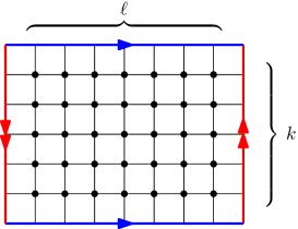
Figure 2. Left: A $k$ by $\ell$ grid on the Klein bottle (the graph itself can be obtained by identifying the two blue segments (in the same direction), and the two red segments (in opposite directions)). Right: The planar triangle-free graph $H_{2\ell}$ (drawn here for $2\ell=4$).

Let $G_{k,\ell}$ denote the $k$ by $\ell$ rectangular grid on the Klein bottle (where $k$ denotes the length of vertical cycles and $\ell$ denotes the length of horizontal cycles, see Figure 2, left). It was proved by Gallai [14] (see also [19, 2]) that for any $k$ and $\ell$, the graph $G_{2k+1,2\ell+1}$ is 4-chromatic. Observe that in $G_{2k+1,2k+1}$, any ball of radius less than $k$ is isomorphic to a ball of the planar rectangular grid of size $2k+1$ by $2k+1$, and in $G_{5,2\ell+1}$, any ball of radius less than $\ell$ is isomorphic to a ball of a planar triangle-free graph (more precisely, a ball in the graph $H_{2\ell}$ depicted in Figure 2, right). Using Observation 2.4, this implies the following.

Theorem 2.5.

No distributed algorithm can 3-color the graph $H_{k}$ in less than $k/2$ rounds. In particular, no distributed algorithm can 3-color every planar triangle-free graph on $n$ vertices in $o(n)$ rounds.

Theorem 2.6.

No distributed algorithm can 3-color the rectangular $k\times k$-grid in the plane in less than $k/2$ rounds. In particular, no distributed algorithm can 3-color every planar bipartite graph on $n$ vertices in $o(\sqrt{n})$ rounds.

It is an interesting problem to find an algorithm of round complexity matching this lower bound in the case of planar bipartite graphs.

Question 2.7.

Is there a distributed algorithm that can 3-color every $n$-vertex planar bipartite graph in $O(\sqrt{n})$ rounds?

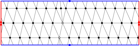
Figure 3. A toroidal triangulation that is not 4-colorable. The graph itself is obtained by identifying the two blue segments, and the two red segments.

Consider now item (1) in Corollary 2.3. It is known that planar graphs are 5-list-colorable [27], so item (1) is not best possible (from an existential point of view). On the other hand, Voigt [28] proved that there exist planar graphs that are not 4-list-colorable. Fisk [12] proved that triangulations of surfaces in which all vertices have even degree except two adjacent vertices, are not 4-colorable. Such triangulations exist in the torus, see Figure 3, where the two vertices of odd degree are depicted in white. Versions of this graph on $n$ vertices clearly exist for any $n\equiv 1\pmod{3}$, and in such a graph any ball of radius at most $\tfrac{n-1}{6}-3$ induces a planar graph. Using Observation 2.4 again, this implies that no distributed algorithm can 4-color every planar graph on $n$ vertices in $o(n)$ rounds, which proves Theorem 1.5. This raises the following natural question.

Question 2.8.

Is it true that there is a distributed algorithm 5-(list-)coloring planar graphs in a polylogarithmic number of rounds?

It might be the case that the girth condition in item (3) of Corollary 2.3 is not best possible, so the following might very well have a positive answer.

Question 2.9.

Is it true that there is a distributed algorithm 3-(list-)coloring planar graphs of girth at least 5 in a polylogarithmic number of rounds?

By the result of Linial [20] (mentioned above), stating that regular trees cannot be colored with a constant number of colors by a distributed algorithm within $o(\log n)$ rounds, there is no hope to obtain a better round complexity for the two questions above.

A possible way to show, as in Theorems 2.5 and 2.6, that planar graphs cannot be efficiently 5-(list-)colored would be to find a graph $G$ embedded on some surface, in which each ball of sufficiently large radius (say $n^{\epsilon}$, for some arbitrary small $\epsilon>0$) is planar, and such that $G$ is not 5-(list-)colorable. However, such a graph does not exist, as we now explain.

Given a graph $G$ embedded in some surface, the edge-width of $G$ is the length of a shortest non-contractible cycle in $G$. The reader is referred to [21] for some background on graphs on surfaces. Note that if $G$ has edge-width at least $2r+2$, then each ball of radius at most $r$ is planar (the converse is not true, as seen for example by considering a 3 by $(2r+2)$ grid on the torus, in which the edge-width is equal to 3, but any $r$-ball is planar). It was proved by Thomassen [26] that any graph embedded in some surface of genus $g$ with edge-width at least $2^{O(g)}$ is 5-colorable. DeVos, Kawarabayashi and Mohar [11] later proved that embedded graphs of sufficiently large edge-width are 5-list-colorable. These results were qualitatively improved recently by Postle and Thomas [25], who showed the following.

Theorem 2.10 ([25]).

If $G$ is embedded in a surface of genus $g$, with edge-width $\Omega(\log g)$, then $G$ is 5-list-colorable. Moreover, if $G$ has girth at least 5, then $G$ is 3-list-colorable.

In their statement, the condition on the edge-width can be replaced by the weaker condition that every ball of radius $O(\log n)$ is planar. Note that any graph on $n$ vertices has genus at most $O(n^{2})$, so it follows that arguments similar to those of Theorem 2.5 and 2.6 cannot prove that planar graphs on $n$ vertices cannot be 5-(list-)colored in $O(\log n)$ rounds. And similarly, the same techniques cannot prove that $n$-vertex graphs of girth at least 5 cannot be $3$-(list)colored in in $O(\log n)$ rounds.

We conclude this section with a consequence of Theorem 1.3 for graphs embeddable on a fixed surface (other than the sphere). A classic result of Heawood states that any graph of Euler genus $g>0$ has maximum average degree at most $\tfrac{1}{2}(5+\sqrt{24g+1})$, and thus choice number at most $H(g)=\lfloor\tfrac{1}{2}(7+\sqrt{24g+1})\rfloor$ (see also [6] and the references therein). Using this bound, we obtain the following direct corollary of Theorem 1.3.

Corollary 2.11.

For any integer $g\geqslant 1$, there is a deterministic distributed algorithm of round complexity $O(\log^{3}n)$ that given an $n$-vertex graph $G$ embeddable on a surface of Euler genus $g$, finds an $H(g)$-list-coloring of $G$. Moreover, when $\tfrac{1}{2}(5+\sqrt{24g+1})$ is an integer and $G$ is not the complete graph on $H(g)$ vertices, the algorithm can indeed find an $(H(g)-1)$-list-coloring of $G$.

If we are merely interested in the existence of such a coloring, the assumption that $\tfrac{1}{2}(5+\sqrt{24g+1})$ is an integer is not necessary in second part of Corollary 2.11, as proved by Böhme, Mohar and Stiebitz [6]. From an algorithmic point of view however, it is not clear whether this assumption can be omitted.

3. Overview of the proof of Theorem 1.3

We now recall the setting of Theorem 1.3. The graph $G$ has $n$ vertices, and maximum average degree at most $d$, for some integer $d\geqslant 3$. Moreover, $G$ does not contain any clique on $d+1$ vertices (otherwise such a clique can be found in two rounds, and we are done). Any vertex $v$ has a list $L(v)$ of $d$ colors, and our goal is to efficiently find an $L$-list-coloring.

A first remark is that we can assume without loss of generality that $d\leqslant n$, since otherwise we can simply set $d:=n$ in the theorem. This will be assumed implicitly throughout the proof (in fact it will only be needed towards the end of the proof of Proposition 4.4).

The proof of Theorem 1.3 goes as follows: in a polylogarithmic number of rounds, we identify some set $A$ of vertices of $G$, representing a constant fraction of the vertex set, and such that any list-coloring of $G-A$ can be extended to $A$ in a polylogarithmic number of rounds. By repeatedly removing such a set $A$ (this can be done at most $O(\log n)$ times), we obtain a trivial graph (that can easily be colored) and then proceed to extend this coloring to each of the sets $A$ that were removed, one by one (starting from the last one to the first one).

So the proof naturally breaks into two very different parts. In the first one, we find such a set $A$ and show that it has size linear in $n$. We use purely graph theoretic arguments but we feel that some of our tools could be useful to design other distributed algorithms. In the second part, we show how to extend any coloring of $G-A$ to $G$ in a polylogarithmic number of rounds. The analysis uses a combination of Theorem 1.1 and classic tools from distributed computing.

Let us now be more specific about the set $A$ mentioned above. Let $c=\tfrac{12}{\log(6/5)}$ (this specific value will only be needed in the proof of Proposition 4.4, so anywhere else in the proof the reader can simply assume that $c$ is any fixed constant). Given a vertex $v$ and an integer $r$, the ball centered in $v$ of radius $r$, denoted by $B^{r}(v)$, is the set of vertices at distance at most $r$ from $v$. We will often consider balls of radius $r=\lceil c\log n\rceil$, in this case we will omit the superscript in $B^{\lceil c\log n\rceil}(v)$ and write $B(v)$ instead. Note that from now on we will omit floors and ceiling when they are not necessary in our discussions (we will write $c\log n$ instead of $\lceil c\log n\rceil$ and consider it as an integer). We will also be interested in balls within specific subgraphs of $G$. Given a subset $R$ of vertices of $G$, $B_{R}^{r}(v)$ is the subset of vertices of $G$ that are at distance at most $r$ from $v$ in $G[R]$ (the subgraph of $G$ induced by $R$). Note that the ball $B_{R}^{r}(v)$ is empty if and only if $v\not\in R$. Again, for convenience, we write $B_{R}(v)$ instead of $B_{R}^{c\log n}(v)$.

Any vertex of degree at most $d$ in $G$ is said to be rich, and the remaining vertices are said to be poor. Note that there are at most $\tfrac{d}{d+1}\,n$ poor vertices, and thus the set $R$ of rich vertices has size at least $\tfrac{n}{d+1}$ (a formal proof will be provided at the end of the proof of Lemma 3.1). Our goal is to select a large set of vertices that can be easily (and efficiently) colored, given a partial coloring of the rest of the graph. Vertices $v$ of degree at most $d-1$ certainly have this property, since their lists contain at least one more color than their degree (and then the coloring of $G-v$ can be extended). However, it might be the case that $G$ contains few such vertices, or even no such vertex at all (if $G$ is $d$-regular), and thus we also have to look for candidates in the set of vertices of degree precisely $d$. Indeed, we will not consider poor vertices (whose degree is at least $d+1$) as possible candidates. The ball $B_{R}(v)$ (as defined in the preceding paragraph) of a rich vertex $v$ is called the rich ball of $v$. A rich vertex is said to be happy if its rich ball $B_{R}(v)$ contains a vertex of degree at most $d-1$ in $G$ or is not a Gallai tree. Recall that this second option is equivalent to the fact that some block (2-connected component) of the subgraph of $G$ induced by $B_{R}(v)$ is neither an odd cycle nor a clique. We denote by $A$ the set of happy vertices. In Section 4, we prove the following result.

Lemma 3.1.

$|A|\geqslant\tfrac{n}{(3d)^{3}}$. Moreover, if there are no poor vertices in $G$, then $|A|\geqslant\tfrac{n}{12d+1}$.

Our goal is then to prove that any coloring of $G-A$ can be efficiently extended to $A$.

Lemma 3.2.

Any $L$-list-coloring of $G-A$ can be extended to an $L$-list-coloring of $G$ in $O(d\log^{2}n)$ rounds.

Lemma 3.2 will be proved in Section 5. In the remainder of this section, we show how to deduce Theorem 1.3 from Lemmas 3.1 and 3.2.

Proof of Theorem 1.3. Since being happy only depends on the ball of radius $c\log n$ around each vertex, the set $A$ of happy vertices can be found in $O(\log n)$ rounds. We repeatedly remove sets $A_{1},A_{2},\ldots,A_{k}$ from $G$ using Lemma 3.1 until $G$ is empty. By Lemma 3.1, $k\leqslant\tfrac{\log n}{\log(1/(1-1/27d^{3}))}=O(d^{3}\log n)$, and thus this part of the procedure takes $O(d^{3}\log^{2}n)$ rounds. If each vertex of $G$ has degree at most $d$, then there are no poor vertices and it follows similarly from Lemma 3.1 that $k=O(d\log n)$ and this part of the procedure takes $O(d\log^{2}n)$ rounds.

We then extend the list-coloring of the empty graph to $A_{k},A_{k-1},\ldots,A_{1}$ using Lemma 3.2. Each extension takes $O(d\log^{2}n)$ rounds, so this part of the procedure runs in $O(kd\log^{2}n)=O(d^{4}\log^{3}n)$ rounds. If each vertex of $G$ has degree at most $d$, this part of the procedure runs in $O(kd\log^{2}n)=O(d^{2}\log^{3}n)$ rounds. In the end, we obtain an $L$-list-coloring of $G$ in $O(d^{4}\log^{3}n)$ rounds (or $O(d^{2}\log^{3}n)$ rounds if $G$ has maximum degree at most $d$), as desired. This concludes the proof of Theorem 1.3. $\Box$

Observe that the proof above basically says that the round complexity in Theorem 1.3 is at most $O(\log n)$ times $O(d\log^{2}n)$ (the complexity of Lemma 3.2) times $O(d^{3})$ or $O(d)$ (the denominators in the bounds of Lemma 3.1). So any improvement in either of these two lemmas would yield an immediate improvement in Theorem 1.3.

4. $A$ has linear size – Proof of Lemma 3.1

The goal of this section is to prove that $A$, the set of happy vertices, has size linear in $n$.

Recall that a vertex is happy if it is rich (i.e. it has degree at most $d$) and its rich ball $B_{R}(v)=B_{R}^{c\log n}(v)$ contains a vertex of degree at most $d-1$ or is not a Gallai tree. Let $S=R\setminus A$ (here ‘S’ stands for ‘Sad’). Note that $S$ is the set of rich vertices whose rich ball contains only vertices of degree $d$ (in $G$) and induces a Gallai tree. We will prove that $S$ is not too large compared to $A$ (Proposition 4.4 below), and since $R=A\cup S$ has size linear in $n$, this will prove Lemma 3.1.

Recall that the girth of a graph $G$ is the length of a shortest cycle in $G$. Note that if $G$ has girth at least $g$, then any ball $B^{\tfrac{g-1}{2}}(v)$ induces a tree (and thus a Gallai tree). We will need a consequence of the following result of Alon, Hoory and Linial [1].

Theorem 4.1 ([1]).

If a graph $G$ has girth at least $g$ ($g$ odd), and average degree $d=2+\delta$, for some real number $\delta>0$, then

$$n\geqslant 1+d\sum_{i=0}^{\tfrac{g-1}{2}}(d-1)^{i}\geqslant(1+\delta)^{\tfrac{g-1}{2}}.$$

We will only use the following direct corollary of Theorem 4.1.

Corollary 4.2.

If an $n$-vertex graph $G$ has girth at least $g$, and average degree at least $2+\delta$, for some real number $\delta>0$, then

$$g\leqslant\tfrac{4}{\log(1+\delta)}\,\log n.$$

Proof.

We can assume that $g$ or $g-1$ is odd, and thus by Theorem 4.1 we have $n\geqslant(1+\delta)^{\tfrac{g}{2}-1}$. It follows that

$$g\leqslant\tfrac{2\log n}{\log(1+\delta)}+2\leqslant\tfrac{4}{\log(1+\delta)}\,\log n,$$

since $1+\delta\leqslant n$. ∎

Note that any induced subgraph of a Gallai tree is also a Gallai tree. Thus, in $G[S]$, all balls of radius $c\log n$ are also Gallai trees. A block of a ball of radius $c\log n$ in $G[S]$ is called a local block of $G[S]$. Observe that if a local block $B$ of $G[S]$ is not a block of $G[S]$, then $B$ is contained in a block of $G[S]$ that contains a cycle of length greater than $2c\log n$. Another important observation about local blocks of $G[S]$ is as follows.

Observation 4.3.

If three vertices $u,v,w$ of a maximal clique $K$ are in a local block of $G[S]$, then $K$ is a local block of $G[S]$.

To see why this holds, observe that in any ball $B(x)$ of $G[S]$ where $u,v,w$ are in a block $C$ of the ball (by definition the ball $B(x)$ induces a Gallai tree, and thus this block $C$ is a clique on at least 3 vertices), some vertex of $C$, say $u$, is closer from $x$ than the others (it is the vertex to which $C$ is attached to the rest of the Gallai tree induced by $B(x)$). Since all the vertices of $K$ are at least as close from $x$ as $v$, $K\subseteq B(x)$ and thus $K=C$ itself is a local block of $G[S]$, which proves Observation 4.3.

The bulk of the proof of Lemma 3.1 is contained in the following technical proposition.

Proposition 4.4.

There are at least $\tfrac{1}{12}\,|S|$ vertices of degree at most $d-1$ in $G[S]$.

Proof.

Let $H$ be the graph obtained from $G[S]$ by doing the following:

• First, for each local block $C$ isomorphic to a clique on at least 3 vertices, we add a vertex $v_{C}$ adjacent to all the vertices of $C$, and then remove all the edges of $C$. By definition, all vertices $v_{C}$ have degree at least 3. These vertices are drawn in white in Figure 4, center and right.

  Note that we might have decreased the degree of some vertices in the process: in particular there might be some vertices of degree at least 3 in $G[S]$ that have degree precisely 2 in the current construction. Let us call $T$ this set of vertices (these vertices are circled in Figure 4, center). Note that each vertex of $T$ has to be adjacent to a vertex $v_{C}$ (for some clique $C$ on at least 3 vertices, and so $v_{C}$ has degree at least 3), and thus there is no path of three consecutive vertices of $T$ in the current construction. Note that since every ball of radius $c\log n$ in $G[S]$ is a Gallai tree, vertices of $T$ are not contained in any cycle of size $2c\log n$.

• Then we suppress all the vertices of $T$. Here, by suppressing a vertex of degree two, we mean deleting this vertex, and then adding an edge between its two neighbors if they are not already adjacent (in other words, we replace a path on 2 edges by a path on 1 edge). Note that if we suppress two adjacent vertices of degree two, this is equivalent to replacing a path on 3 edges by a path on 1 edge. A direct consequence of the final remark in the paragraph above is that $H$ has girth at least 5 (in particular the construction does not produce loops or multiple edges).

The two steps of the construction of $H$ are depicted in Figure 4.

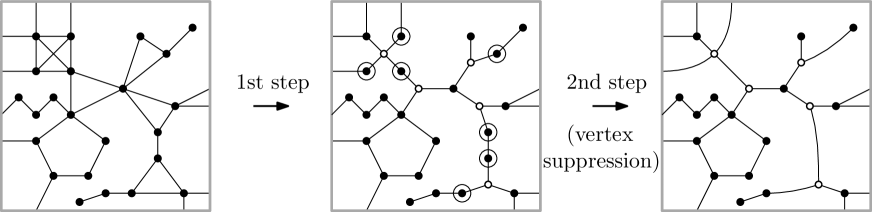
Figure 4. The two-step construction of $H$ from $G[S]$ (viewed from a ball of radius $c\log n$).

Observe that if a vertex $v$ of $G[S]$ has degree at least 3 in $G[S]$ and at most 2 in $H$, then it follows from our vertex suppression step that $v$ has degree at most 1 in $H$. Such a vertex $v$ thus lies in a unique local block $B$ in $G[S]$, which is a clique on at least 3 vertices. Since cliques have size at most $d$ in $G$, such a vertex $v$ has degree at most $d-1$ in $G[S]$. Since $d\geqslant 3$, it follows that the number of vertices of degree at most $d-1$ in $G[S]$ is at least the number of vertices of degree at most 2 in $H$. Hence, to prove the theorem it is enough to show that there are at least $\tfrac{1}{12}\,|S|$ vertices of degree at most 2 in $H$.

Before proving this, let us do two convenient observations on the number of vertices and the size of cycles in $H$.

• Since each vertex of $R$ has degree at most $d$, each vertex of $S$ lies in at most $d/2$ cliques of at least 3 vertices which are local blocks. Indeed, (i) an edge cannot be in two distinct maximal cliques by inclusion, otherwise the ball of radius one centered on one of the vertices of the edge would not be a Gallai tree, contradicting the fact that it is in $S$. And (ii) local blocks which are cliques of size at least $3$ are maximal by inclusion by Observation 4.3. Thus $H$ contains at most $(1+\tfrac{d}{6})\,|S|\leqslant\tfrac{d}{2}\,|S|$ vertices (here we used that $d\geqslant 3$).

• Consider any cycle $C$ of length $\ell$ in $H$. By construction, $C$ is either a local block of $G[S]$ (in which case $\ell$ is odd and $5\leqslant\ell\leqslant 2c\log n$, since triangles are considered as cliques on 3 vertices and every edge is in at most one local block which is a clique as we already observed in the previous point), or corresponds to a cycle of $G[S]$ of length at least $\ell/3$ that is not contained in any ball of radius $c\log n$ of $G[S]$. The bound $\ell/3$ follows from the fact that there were no paths of 3 vertices of $T$ before the suppression step, and thus we have only replaced paths on 2 or 3 edges by single edges. It follows that any cycle of $H$ distinct from a local block of $G[S]$ has length greater than $\tfrac{2c}{3}\log n$.

Let $H^{\prime}$ be the graph obtained from $H$ by removing precisely one edge in each cycle of length between 5 and $\tfrac{2c}{3}\log n$. Note that the observation above ensures that such a cycle is necessarily a local block of $G[S]$, and is thus an induced odd cycle. Such cycles are pairwise edge-disjoint otherwise any vertex incident to an edge lying in the intersection of two such cycles would be happy. It follows from the construction that $H^{\prime}$ has girth greater than $\tfrac{2c}{3}\log n$. Since each cycle of $H$ contains at least 5 edges, we have removed at most a fifth of the edges of $H$, and thus the average degree of $H$ is at most $\tfrac{5}{4}$ times the average degree of $H^{\prime}$.

Assume for the sake of contradiction that $H^{\prime}$ has average degree at least $\tfrac{11}{5}$. Applying Corollary 4.2 to the graph $H^{\prime}$ with $g>\tfrac{2c}{3}\log n$ and $\delta=\tfrac{1}{5}$, we obtain $\tfrac{2c}{3}\log n<\tfrac{4}{\log(6/5)}\,\log|V(H)|\leqslant\tfrac{4}{\log(6/5)}\,\log\tfrac{d|S|}{2}\leqslant\tfrac{8}{\log(6/5)}\,\log n$, using that $d\leqslant n$ and $|S|\leqslant n$. This implies that $c<\tfrac{12}{\log(6/5)}$, which contradicts our definition of $c$. We can thus assume that $H^{\prime}$ has average degree at most $\tfrac{11}{5}$, and thus $H$ has average degree at most $\tfrac{5}{4}\cdot\tfrac{11}{5}=\tfrac{11}{4}$. It follows that $H$ has at least $|S|/12$ vertices of degree at most two, and thus $G[S]$ has at least $|S|/12$ vertices of degree at most $d-1$, which concludes the proof of Proposition 4.4. ∎

We are now ready to prove Lemma 3.1.

Proof of Lemma 3.1. By Proposition 4.4, there are at least $\tfrac{1}{12}\,|S|$ vertices of degree at most $d-1$ in $G[S]$. Since each vertex of $S$ has degree $d$ in $G$, this implies that there are also at least $\tfrac{1}{12}\,|S|$ edges leaving $S$. Let us divide these edges into two sets: $E(S,P)$, the set of edges with one end in $S$ and the other in $P$, the set of poor vertices, and $E(S,A)$, the set of edges with one end in $S$ and the other in $A$. Observe that since each vertex of $A$ has degree at most $d$, we have $|A|\geqslant\tfrac{1}{d}|E(S,A)|$.

Since $G$ has average degree at most $d$, we have $\sum_{v\in G}(d_{G}(v)-d)\leqslant 0$. Recall that $P$ (the set of poor vertices) is precisely the set of vertices of degree at least $d+1$ in $G$, while $A$ (the set of happy vertices) contains all the vertices of degree at most $d-1$ in $G$, and thus

$$d|A|\geqslant\sum_{v\in A}(d-d_{G}(v))\geqslant\sum_{v\in P}(d_{G}(v)-d)\geqslant\max(|P|,|E(S,P)|-d|P|).$$

It follows that $|E(S,P)|\leqslant d|P|+d|A|\leqslant d(d+1)|A|$, and thus $|A|\geqslant\tfrac{1}{d(d+1)}|E(S,P)|$.

Summing up the inequalities we obtained on $|E(S,A)|$ and $|E(S,P)|$, we obtain

$$|A|(1+\tfrac{1}{d+1})\geqslant|A|+\tfrac{1}{d+1}|A|\geqslant\tfrac{1}{d(d+1)}(|E(S,P)|+|E(S,A)|)\geqslant\tfrac{|S|/12}{d(d+1)},$$

and thus $|A|\geqslant\tfrac{|S|}{12d(d+2)}$.

Since $G$ has average degree at most $d$, the set $R=A\cup S$ contains at least $\tfrac{n}{d+1}$ vertices and thus

$$|A|\geqslant\tfrac{n}{(d+1)(12d(d+2)+1)}\geqslant\tfrac{n}{(3d)^{3}},$$

where we used that $d\geqslant 3$ in the last inequality. This concludes the proof of the first part of Lemma 3.1.

Assume now that $G$ has maximum degree at most $d$. Then $P$ is empty, and so is $E(S,P)$. It follows that $|A|\geqslant\tfrac{1}{d}|E(S,A)|\geqslant\tfrac{1}{12d}\,|S|$. Since $P$ is empty, $V(G)=R=A\cup S$ and thus $|A|\geqslant\tfrac{n}{12d+1}$, as desired. This concludes the proof of Lemma 3.1. $\Box$

5. The coloring can be extended efficiently – Proof of Lemma 3.2

The goal of this section is to prove that any $L$-list-coloring of $G-A$ can be efficiently extended to $A$. (Actually our recoloring process might modify the colors of some vertices of $G\setminus A$). To show this, we will need the notion of an $(\alpha,\beta)$-ruling forest, introduced by Awerbuch et al. in [3]. Given a graph $H$ and a subset $U$ of vertices of $H$, an $(\alpha,\beta)$-ruling forest with respect to $U$ is a family of vertex-disjoint rooted trees $(T_{i},r_{i})_{1\leqslant i\leqslant t}$, such that

1. each vertex of $U$ lies in some tree $T_{i}$, and

2. for each $1\leqslant i<j\leqslant t$, the roots $r_{i}$ and $r_{j}$ are at distance at least $\alpha$ in $H$, and

3. each rooted tree $T_{i}$ has depth at most $\beta$ (i.e. each vertex of $T_{i}$ is at distance at most $\beta$ from $r_{i}$ in $T_{i}$).

Awerbuch et al. in [3] proved that a $(k,k\log n)$-ruling forest can be computed deterministically in the LOCAL model in a graph on at most $n$ vertices in $O(k\log n)$ rounds. Note that ruling forests were also used by Panconesi and Srinivasan [23] in their “distributed” proof of Brooks theorem, but our application here is slightly different, essentially due to the fact that we have to consider a list-coloring problem rather than a coloring problem (and it is seems that their approach of switching colors cannot be applied in the list-coloring framework).

Consider a graph $G^{\prime}$, in which every vertex $v$ starts with a list $L^{\prime}(v)$ of size $d$, and assume that a subset $U$ of vertices is precolored (i.e. each vertex of $u$ is assigned a color from its list). Let $H$ be the subgraph of $G$ induced by the uncolored vertices (i.e. the vertices outside $U$), and for each $v\in H$, let $L_{H}(v)$ be the list obtained from $L^{\prime}(v)$ by removing the colors of the precolored neighbors of $v$. Recall that $d_{H}(v)$ denotes the degree of a vertex $v$ in $H$. The following simple observation will be crucial in our proof Lemma 3.2.

Observation 5.1.

For any vertex $v\in H$, $|L_{H}(v)|\geqslant d-d_{G^{\prime}}(v)+d_{H}(v)$. In particular, if $d_{G^{\prime}}(v)\leqslant d$ then $|L_{H}(v)|\geqslant d_{H}(v)$ and if $d_{G^{\prime}}(v)\leqslant d-1$ then $|L_{H}(v)|\geqslant d_{H}(v)+1$.

We can now proceed with the proof of Lemma 3.2.

Proof of Lemma 3.2. Recall that the vertex-set $G$ is divided into two sets: $R$, the rich vertices (that have degree at most $d$), and $P$, the poor vertices (that have degree at least $d+1$) and the set $R$ itself is divided into $A$ (the happy vertices), and $S$ (the set of rich vertices whose rich ball of radius $c\log n$ induces a Gallai tree and only contains vertices of degree $d$ in $G$).

Consider some $L$-list-coloring of $G-A$, which we wish to extend to $A$.

Let $(T_{i},r_{i})_{1\leqslant i\leqslant t}$ be a $(k,k\log n)$-ruling forest in $G[R]$ with respect to $A$, with $k=2c\log n$. This ruling forest can be computed in $O(\log^{2}n)$ rounds as proved in [3]. Let us denote by $T$ the union of the vertices contained in some tree $T_{i}$. Note that $T$ contains $A$ (the set of vertices that are uncolored at this point), and also possibly some (colored) vertices of $S$. We uncolor all the vertices of $T\cap S$, and now $T$ is precisely the set of uncolored vertices.

Let $H$ be the subgraph of $G$ induced by $T$. For each vertex $v\in T$, we start by removing from $L(v)$ the colors of the neighbors of $v$ outside $T$. Let us denote by $L_{H}(v)$ the new list of each vertex $v$ of $H$ after this removal step. By construction, in order to extend the coloring of $G-A$ to $A$ it is enough to (efficiently) find an $L_{H}$-list-coloring of $H$.

Since each vertex $v\in T$ has degree at most $d$ in $G$, and starts with a list $L(v)$ of size $d$, it follows from Observation 5.1 that $|L_{H}(v)|\geqslant d_{H}(v)$. To find an $L_{H}$-list-coloring of $H$, we first compute a partition of $H$ into $d+1$ stable sets $C_{1},C_{2},\ldots,C_{d+1}$. Since each vertex of $T$ has degree at most $d$ in $G$ and thus in $H$, such a partition (which is exactly a proper $(d+1)$-coloring) can be computed deterministically in $O(d\log n)$ rounds [17]. Recall that each tree $T_{i}$ has depth at most $k\log n=2c\log^{2}n$. We then proceed to $L_{H}$-list-color $H$ as follows: for each $i$ from $2c\log^{2}n$ to 1, and for each $j$ from 1 to $d+1$, we consider the vertices of $C_{j}$ that are at distance precisely $i$ from the root of their respective tree of the ruling forest (these vertices form a stable set of $H$ and can thus be colored independently), and each of these vertices selects a color of its list $L_{H}$ that does not appear on any of its colored neighbors in $H$. Since each such vertex $v$ has at least one uncolored neighbor in $H$ (its parent in the ruling forest, since we proceed from the leaves to the root), it has at most $d_{H}(v)-1\leqslant|L_{H}(v)|-1$ colored neighbors and can thus select a suitable color from its list.

This procedure takes $O(d\log^{2}n)$ steps, and all that remains to do is to find suitable colors for the roots $r_{i}$, $1\leqslant i\leqslant t$. By the definition of a ruling forest, each root $r_{i}$ lies in $A$, and thus the ball $B_{R}(r_{i})$ (of radius $c\log n$) contains a vertex of degree at most $d-1$ or is not a Gallai tree. Moreover, it also follows from the defintion of our ruling forest that any two balls $B_{R}(r_{i})$ and $B_{R}(r_{j})$ are disjoint and have no edges between them. We then uncolor each of the balls $B_{R}(r_{i})$ completely, and remove from the lists of the vertices inside these balls the colors assigned to their neighbors outside the balls. As before, it follows from Observation 5.1 that the list of remaining colors of each vertex $v$ is as least as large as the number of uncolored neighbors of $v$. Moreover, if $v$ has degree at most $d-1$ in $G$, the list of remaining colors for $v$ is strictly larger than the number of uncolored neighbors of $v$. It thus follows from the definition of $A$ that each vertex $r_{i}$ can apply Theorem 1.1 to its ball $B_{R}(r_{i})$, and thus extend the current $L_{H}$-list-coloring to these balls in $k\log n=2c\log^{2}n=O(\log^{2}n)$ additional steps. This concludes the proof of Lemma 3.2. $\Box$

6. Conclusion

In Theorem 1.3, every vertex has the same number of colors in its list. However, as seen in Theorem 1.1, in the list-coloring setting, some results can be obtained when vertices have a varying number of colors. Indeed, many distributed $(\Delta+1)$-coloring algorithms work in the more general $(\mbox{deg}+1)$-list-coloring setting, where each vertex $v$ is given a list of $d(v)+1$ colors, and the complexity of this specific problem plays an important role in the most efficient distributed $(\Delta+1)$-coloring algorithms to date [8, 18].

There are obvious obstacles to an efficient version of Theorem 1.1 in the distributed setting: we cannot apply it to paths in $o(n)$ rounds. Paths are not the only difficult case to circumvent, as one could attach a clique to every vertex on a path and face similar issues. Therefore, we need to assume that every vertex $v$ has a list $L(v)$ of size $d(v)$, except if $d(v)\leqslant 2$ or the neighbors of $v$ form a clique, in which cases $v$ has a list $L(v)$ of size $d(v)+1$. Such a list-assignment $L$ is said to be nice. The same algorithm and proof go through merely by replacing $d$ with the size of the given vertex’ list. Indeed, every vertex is rich, and thus we obtain a complexity of $O(\Delta^{2}\log^{3}n)$ rounds.

Theorem 6.1.

There is a deterministic distributed algorithm that given an $n$-vertex graph $G$ of maximum degree $\Delta$, and a nice list-assignment $L$ for the vertices of $G$, finds an $L$-list-coloring of $G$ in $O(\Delta^{2}\log^{3}n)$ rounds.

We note that this also implies Corollary 2.1 and is another way to refine the result by Panconesi and Srinivasan [23] (which is faster by a factor of $\Delta\log\Delta$).

To conclude, observe that a major difference between coloring and list-coloring in the distributed setting is that finding some coloring is easy (each vertex chooses its own identifier), while finding some list-coloring might be non trivial. This raises the following intriguing question, which does not seem to have been considered before (to the best of our knowledge).

Question 6.2.

Given an $n$-vertex graph $G$, in which each vertex has a list of $n$ available colors, is there a simple deterministic distributed algorithm list-coloring $G$ in, say, $O(\log n)$ rounds?

Remark that there is a simple answer to Question 6.2 if we ask for a randomized algorithm instead (see for instance [5] for the description of a simple randomized distributed $(\Delta+1)$-coloring algorithm in $O(\log n)$ rounds, which can be easily adapted to work in the list-coloring setting).

Recent developments

Since we made our manuscript public, two papers on close topics appeared.

In [15], the authors were interested in $d$-coloring non-complete graphs of maximum degree at most $d$ (this corresponds to the setting of our Corollary 2.1). They gave a deterministic distributed algorithm with round complexity $O(d^{1/2}\log^{2}n)$ (improving our bound of $O(d^{2}\log^{3}n)$), and a randomized distributed algorithm with round complexity $d^{1/2+o(1)}(\log\log n)^{2}$. Using known lower bounds on the round complexity of the deterministic version of the problem (essentially $\Omega(\log n)$), this implies an exponential separation between the deterministic and randomized versions of the problem.

In [9], the authors were interested specifically in planar graphs. They gave deterministic distributed algorithms to 4-color triangle-free planar graphs and 6-color planar graphs in $O(\log n)$ rounds (improving our round complexity of $O(\log^{3}n)$ from Corollary 2.3). They also gave a different proof of Theorem 1.5.

Acknowledgments.

The authors would like to thank Leonid Barenboim and Michael Elkin for the discussion about the parallel 5-coloring algorithm for planar graphs of [17] mentioned in [4], Jukka Suomela for providing helpful references, Cyril Gavoille for his comments and suggestions, and Zdeněk Dvořák and Luke Postle for the discussions about coloring embedded graphs of large edge-width.

References

- [1] N. Alon, S. Hoory and N. Linial, The Moore bound for irregular graphs, Graphs Combin. 18 (2002), 53–57.
- [2] D. Archdeacon, J. Hutchinson, A. Nakamoto, S. Negami, and K. Ota, Chromatic Numbers of Quadrangulations on Closed Surfaces, J. Graph Theory 37 (2001), 100–114.
- [3] B. Awerbuch, A.V. Goldberg, M. Luby, and S. Plotkin, Network decomposition and locality in distributed computation, In Proc. of the 30th Annual Symposium on Foundations of Computer Science (1989), 364–369.
- [4] L. Barenboim and M. Elkin, Sublogarithmic distributed MIS algorithm for sparse graphs using Nash-Williams decomposition, Distributed Computing 22(5-6) (2010), 363–379.
- [5] L. Barenboim and M. Elkin, Distributed graph coloring: Fundamentals and recent developments, Synthesis Lectures on Distributed Computing Theory 4(1) (2013), 1–171.
- [6] T. Böhme, B. Mohar, and M. Stiebitz, Dirac’s map-color theorem for choosability, J. Graph Theory 32 (1999), 327–339.
- [7] O. Borodin, Criterion of chromaticity of a degree prescription, In Abstracts of IV All-Union Conf. on Th. Cybernetics (1977), 127–128.
- [8] Y.-J. Chang, W. Li, and S. Pettie, An optimal distributed -coloring algorithm?, In Proc. of the 50th ACM Symposium on Theory of Computing (STOC), 2018.
- [9] S. Chechik and D. Mukhtar, Optimal Distributed Coloring Algorithms for Planar Graphs in the LOCAL model, In Proc. of the ACM-SIAM Symposium on Discrete Algorithms (SODA), 2019.
- [10] P. Erdős, A. Rubin, and H. Taylor, Choosability in graphs, In Proc. West Coast Conf. on Combinatorics, Graph Theory and Computing, Congressus Numerantium 26 (1979), 125–157.
- [11] M. DeVos, K. Kawarabayashi, B. Mohar, Locally planar graphs are 5-choosable, J. Combin. Theory Ser. B 98 (2008), 1215–1232.
- [12] S. Fisk, The non-existence of colorings, J. Combin. Theory Ser. B 24 (1978), 247–248.
- [13] H. Grötzsch, Ein Dreifarbensatz für dreikreisfreie Netze auf der Kugel, Wiss. Z. Martin-Luther-Univ. Halle-Wittenberg Math.-Natur. Reihe 8 (1959), 109–120.
- [14] T. Gallai, Kritische Graphen I, Magyar Tud. Akad. Mat. Kutakó Int. Közl 8 (1963), 165–192.
- [15] M. Ghaffari, J. Hirvonen, F. Kuhn, and Y. Maus, Improved Distributed -Coloring, ACM Symposium on Principles of Distributed Computing (PODC), 2018.
- [16] M. Ghaffari and C. Lymouri, Simple and Near-Optimal Distributed Coloring for Sparse Graphs, International Symposium on Distributed Computing (DISC) 2017.
- [17] A. Goldberg, S. Plotkin, and G. Shannon, Parallel symmetry-breaking in sparse graphs, SIAM J. Discrete Math. 1(4) (1988), 434–446.
- [18] D. Harris, J. Schneider, and H.-H. Su, Distributed -coloring in sublogarithmic rounds, In Proc. of the 48th ACM Symposium on Theory of Computing (STOC) 2016, 465–478.
- [19] S. Klavžar and B. Mohar, The chromatic numbers of graph bundles over cycles, Discrete Math. 138 (1995), 301–314.
- [20] N. Linial, Locality in distributed graph algorithms, SIAM J. Comput. 21 (1992), 193–201.
- [21] B. Mohar and C. Thomassen, Graphs on Surfaces. Johns Hopkins University Press, Baltimore, 2001.
- [22] C.St.J.A. Nash-Williams, Decomposition of finite graphs into forests, J. London Math. Soc. 1(1) (1964), 12–12.
- [23] A. Panconesi, and A. Srinivasan, The local nature of -coloring and its algorithmic applications, Combinatorica 15 (1995), 255–280.
- [24] A. Panconesi and A. Srinivasan, On the complexity of distributed network decomposition, J. Algor. 20(2) (1996), 356–374.
- [25] L. Postle and R. Thomas, Hyperbolic families and coloring graphs on surfaces, Manuscript, 2016. ArXiv:1609.06749
- [26] C. Thomassen, Five-coloring maps on surfaces, J. Combin. Theory Ser. B 59 (1993), 89–105.
- [27] C. Thomassen, Every planar graph is 5-choosable, J. Combin. Theory Ser. B 62 (1994), 180–181.
- [28] M. Voigt, List colourings of planar graphs, Discrete Math. 120 (1993), 215–219.
- [29] M. Voigt, A not 3-choosable planar graph without 3-cycles, Discrete Math. 146 (1995), 325–328.