Optimal Transport: Fast Probabilistic Approximation with Exact Solvers

Abstract

We propose a simple subsampling scheme for fast randomized approximate computation of optimal transport distances on finite spaces. This scheme operates on a random subset of the full data and can use any exact algorithm as a black-box back-end, including state-of-the-art solvers and entropically penalized versions. It is based on averaging the exact distances between empirical measures generated from independent samples from the original measures and can easily be tuned towards higher accuracy or shorter computation times. To this end, we give non-asymptotic deviation bounds for its accuracy in the case of discrete optimal transport problems. In particular, we show that in many important instances, including images (2D-histograms), the approximation error is independent of the size of the full problem. We present numerical experiments that demonstrate that a very good approximation in typical applications can be obtained in a computation time that is several orders of magnitude smaller than what is required for exact computation of the full problem.

1 Introduction

Optimal transport distances, a.k.a. Wasserstein, earth-mover’s, Monge-Kantorovich-Rubinstein or Mallows distances, as metrics to compare probability measures (Rachev and Rüschendorf, 1998; Villani, 2008) have become a popular tool in a wide range of applications in computer science, machine learning and statistics. Important examples are image retrieval (Rubner et al., 2000) and classification (Zhang et al., 2007), computer vision (Ni et al., 2009), but also therapeutic equivalence (Munk and Czado, 1998), generative modeling (Bousquet et al., 2017), biometrics (Sommerfeld and Munk, 2018), metagenomics (Evans and Matsen, 2012) and medical imaging (Ruttenberg et al., 2013).

Optimal transport distances compare probability measures by incorporating a suitable ground distance on the underlying space, typically driven by the particular application, e.g. euclidean distance. This often makes it preferable to competing distances such as total-variation or $\chi^{2}$-distances, which are oblivious to any metric or similarity structure on the ground space. Note that total variation is the Wasserstein distance with respect to the trivial metric, which usually does not carry the geometry of the underlying ground space. In this setting, optimal transport distances have a clear and intuitive interpretation as the amount of ‘work’ required to transport one probability distribution onto the other. This notion is typically well-aligned with human perception of similarity (Rubner et al., 2000).

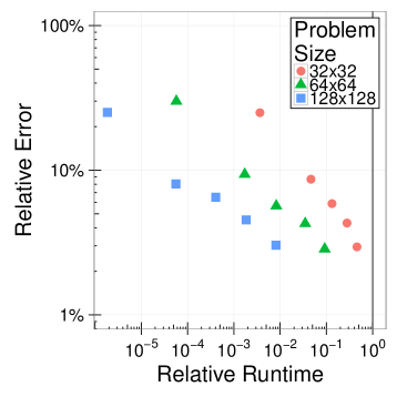
Figure 1: Relative error and relative runtime compared to the exact computation of the proposed scheme. Optimal transport distances and its approximations were computed between images of different sizes ($32\times 32$, $64\times 64$, $128\times 128$). Each point represents a specific parameter choice in the scheme and is a mean over different problem instances, solvers and cost exponents. For the relative runtimes the geometric mean is reported. For details on the parameters see Figure 2.

1.1 Computation

The outstanding theoretical and practical performance of optimal transport distances is contrasted by its excessive computational cost. For example, optimal transport distances can be computed with an auction algorithm (Bertsekas, 1992). For two probability measures supported on $N$ points this algorithm has a worst case run time of $\mathcal{O}(N^{3}\log N)$. Other methods like the transportation simplex have sub-cubic empirical average runtime (compare Gottschlich and Schuhmacher (2014)), but exponential worst case runtimes.

Therefore, many attempts have been made to design improved algorithms. We give some selective references: Ling and Okada (2007) proposed a specialized algorithm for $L_{1}$-ground distance and $\mathcal{X}$ a regular grid and report an empirical runtime of $\mathcal{O}(N^{2})$.Gottschlich and Schuhmacher (2014) improved existing general purpose algorithms by initializing with a greedy heuristic. Their Shortlist algorithm achieves an empirical average runtime of the order $\mathcal{O}(N^{5/2})$. Schmitzer (2016) solves the optimal transport problem by solving a sequence of sparse problems. The theoretical runtime of his algorithm is not known, but it exhibits excellent performance on two-dimensional grids (Schrieber et al., 2016). The literature on this topic is rapidly growing and we refer for further recent work to Liu et al. (2018), Dvurechensky et al. (2018), Lin et al. (2019), and the references given there.

Despite these efforts, still many practically relevant problems remain well outside the scope of available algorithms. See Schrieber et al. (2016) for an overview and a numerical comparison of state-of-the-art algorithms for discrete optimal transport. This is true in particular for two or three dimensional images and spatio temporal imaging, which constitute an important area of potential applications. Here, $N$ is the number of pixels or voxels and is typically of size $10^{5}$ to $10^{7}$. Naturally, this problem is aggravated when many distances have to be computed as is the case for Wasserstein barycenters (Agueh and Carlier, 2011; Cuturi and Doucet, 2014), which have become an important use case.

To bypass the computational bottleneck, also many surrogates for optimal transport distances that are more amenable to fast computation have been proposed. Shirdhonkar and Jacobs (2008) proposed to use an equivalent distance based on wavelets that can be computed in linear time but cannot be calibrated to approximate the Wasserstein distance with arbitrary accuracy. Pele and Werman (2009) threshold the ground distance to reduce the complexity of the underlying linear program, obtaining a lower bound for the exact distance. Cuturi (2013) altered the optimization problem by adding an entropic penalty term in order to use faster and more stable algorithms, see also Altschuler et al. (2017). Bonneel et al. (2015) consider the 1-D Wasserstein distances of radial projections of the original measures, exploiting the fact that, in one dimension, computing the Wasserstein distance amounts to sorting the point masses and hence has quasi-linear computation time.

1.2 Contribution

We do not propose a new algorithm to solve the optimal transport problem. Instead, we propose a simple probabilistic scheme as a meta-algorithm that can use any algorithm (e.g., those mentioned above) solving finitely supported optimal transport problems as a black-box back-end and gives a random but fast approximation of the exact distance. This scheme

1. is extremely easy to implement, to parallelize and to tune towards higher accuracy or shorter computation time as desired;

2. can be used with any algorithm for transportation problems as a back-end, including general LP solvers, specialized network solvers and algorithms using entropic penalization (Cuturi, 2013);

3. comes with theoretical non-asymptotic guarantees for the approximation error of the Wasserstein distance — in particular, this error is independent of the size of the original problem in many important cases, including images;

4. works well in practice. For example, the Wasserstein distance between two $128^{2}$-pixel images can typically be approximated with a relative error of less than $5\%$ in only $1\%$ of the time required for exact computation.

2 Problem and Algorithm

Although our meta-algorithm is applicable to exact solvers for any optimal transport distance between probability measures, for example the Sinkhorn distance (Cuturi, 2013), the theory we present here concerns the Kantorovich (1942) transport distance, often also denoted as Wasserstein distance.

Wasserstein Distance

Consider a fixed finite space $\mathcal{X}=\left\{x_{1},\dots,x_{N}\right\}$ with a metric $d:\mathcal{X}\times\mathcal{X}\rightarrow[0,\infty)$. Every probability measure on $\mathcal{X}$ is given by a vector $\bm{r}$ in

$$\mathcal{P}_{\mathcal{X}}=\left\{\bm{r}=(r_{x})_{x\in\mathcal{X}}\in\mathbb{R}_{\geq 0}^{\mathcal{X}}:\sum_{x\in\mathcal{X}}r_{x}=1\right\},$$

via $P_{\bm{r}}(\{x\})=r_{x}$. We will not distinguish between the vector $\bm{r}$ and the measure it defines. For $p\geq 1$, the $p$-th Wasserstein distance between two probability measures $\bm{r},\bm{s}\in\mathcal{P}_{\mathcal{X}}$ is defined as

$$W_{p}(\bm{r},\bm{s})=\left(\min_{\bm{w}\in\Pi(\bm{r},\bm{s})}\sum_{x,x^{\prime}\in\mathcal{X}}d^{p}\!(x,x^{\prime})w_{x,x^{\prime}}\right)^{1/p},$$ (1)

where $\Pi(\bm{r},\bm{s})$ is the set of all probability measures on $\mathcal{X}\times\mathcal{X}$ with marginal distributions $\bm{r}$ and $\bm{s}$, respectively. The minimization in (1) can be written as a linear program

$$\min\sum_{x,x^{\prime}\in\mathcal{X}}w_{x,x^{\prime}}d^{p}\!(x,x^{\prime})\quad\textbf{s.t.}\quad\sum_{x^{\prime}\in\mathcal{X}}w_{x,x^{\prime}}=r_{x},\quad\sum_{x\in\mathcal{X}}w_{x,x^{\prime}}=s_{x^{\prime}},\quad w_{x,x^{\prime}}\geq 0,$$ (2)

with $N^{2}$ variables $w_{x,x^{\prime}}$ and $2N$ constraints, where the weights $d^{p}\!(x,x^{\prime})$ are known and have been precalculated.

2.1 Approximating the Wasserstein Distance

The idea of the proposed algorithm is to replace a probability measure $\bm{r}\in\mathcal{P}(\mathcal{X})$ with an empirical measure $\hat{\bm{r}}_{S}$ based on i.i.d. picks $X_{1},\dots,X_{S}\sim\bm{r}$ for some integer $S$:

$$\hat{r}_{S,x}=\frac{1}{S}\#\left\{k:X_{k}=x\right\},\quad x\in\mathcal{X}.$$ (3)

Likewise, replace $\bm{s}$ with $\hat{\bm{s}}_{S}$. Then, use the empirical optimal transport distance (EOT) $W_{p}(\hat{\bm{r}}_{S},\hat{\bm{s}}_{S})$ as a random approximation of $W_{p}(\bm{r},\bm{s})$.

Algorithm 1 Statistical approximation of $W_{p}(\bm{r},\bm{s})$

1:  Input: Probability measures $\bm{r},\bm{s}\in\mathcal{P}_{\mathcal{X}}$, sample size $S$ and number of repetitions $B$

2:  for $i=1\dots B$ do

3:     Sample i.i.d. $X_{1},\dots,X_{S}\sim\bm{r}$ and independently $Y_{1},\dots,Y_{S}\sim\bm{s}$

4:     $\hat{r}_{S,x}\leftarrow\#\left\{k:X_{k}=x\right\}/S$ for all $x\in\mathcal{X}$

5:     $\hat{s}_{S,x}\leftarrow\#\left\{k:Y_{k}=x\right\}/S$ for all $x\in\mathcal{X}$

6:     Compute $\hat{W}^{(i)}\leftarrow W_{p}(\hat{\bm{r}}_{S},\hat{\bm{s}}_{S})$

7:  end for

8:  Return: $\hat{W}^{(S)}_{p}(\bm{r},\bm{s})\leftarrow B^{-1}\sum_{i=1}^{B}\hat{W}^{(i)}$

In each of the $B$ iterations in Algorithm 1, the Wasserstein distance between two sets of $S$ point masses has to be computed. For the exact Wasserstein distance, two measures on $N$ points need to be compared. If we take for example the super-cubic runtime of the auction algorithm as a basis, Algorithm 1 has worst case runtime

$$\mathcal{O}(BS^{3}\log S)$$

compared to $\mathcal{O}(N^{3}\log N)$ for the exact distance. This means a dramatic reduction of computation time if $S$ (and $B$) are small compared to $N$.

The application of Algorithm 1 to other optimal transport distances is straightforward. One can simply replace $W_{p}(\hat{\bm{r}}_{S},\hat{\bm{s}}_{S})$ with the desired distance, e.g., the Sinkhorn distance (Cuturi, 2013), see also our numerical experiments below. Further, the algorithm can be applied to non-discrete instances as long as we can sample from the measures. However, the theoretical results below only apply to the EOT on a finite ground space $\mathcal{X}$.

3 Theoretical results

We give general non-asymptotic guarantees for the quality of the approximation $\hat{W}^{(S)}_{p}(\bm{r},\bm{s})=B^{-1}\sum_{i=1}^{B}W_{p}(\hat{\bm{r}}_{S,i},\hat{\bm{s}}_{S,i})$ (where $\hat{\bm{r}}_{S,i}$ are independent empirical measures of size $S$ from $\bm{r}$; see Algorithm 1) in terms of the expected $L_{1}$-error. That is, we give bounds of the form

$$E\left[\left|\hat{W}^{(S)}_{p}(\bm{r},\bm{s})-W_{p}(\bm{r},\bm{s})\right|\right]\leq g(S,\mathcal{X},p),$$ (4)

for some function $g$. We are particularly interested in the dependence of the bound on the size $N$ of $\mathcal{X}$ and on the sample size $S$ as this determines how the number of sampling points $S$ (and hence the computational effort of Algorithm 1) must be increased for increasing problem size $N$ in order to retain (on average) a certain approximation quality. In a second step, we obtain deviation inequalities for $\hat{W}^{(S)}(\bm{r},\bm{s})$ via concentration of measure techniques.

Related work

The question of the convergence of empirical measures to the true measure in expected Wasserstein distance has been considered in detail by Boissard and Le Gouic (2014) and Fournier and Guillin (2015). The case of the underlying measures being different (that is, the convergence of $EW_{p}(\hat{\bm{r}}_{S},\hat{\bm{s}}_{S})$ to $W_{p}(\bm{r},\bm{s})$ when $\bm{r}\neq\bm{s}$) has not been considered to the best of our knowledge. Theorem 1 is reminiscent of the main result of Boissard and Le Gouic (2014). However, we give a result here, which is explicitly tailored to finite spaces and makes explicit the dependence of the constants on the size $N$ of the underlying set $\mathcal{X}$. In fact, when we consider finite spaces $\mathcal{X}$ which are subsets of $\mathbb{R}^{D}$ later in Theorem 3, we will see that in contrast to the results of Boissard and Le Gouic (2014), the rate of convergence (in $S$) does not change when the dimension gets large, but rather the dependence of the constants on $N$ changes. This is a valuable insight as our main concern here is how the subsample size $S$ (driving the computational cost) must be chosen when $N$ grows in order to retain a certain approximation quality.

3.1 Expected absolute error

Recall that, for $\delta>0$ the covering number $\mathcal{N}(\mathcal{X},\delta)$ of $\mathcal{X}$ is defined as the minimal number of closed balls with radius $\delta$ and centers in $\mathcal{X}$ that is needed to cover $\mathcal{X}$. Note that in contrast to continuous spaces, $\mathcal{N}(\mathcal{X},\delta)$ is bounded by$N$ for all $\delta>0$.

Theorem 1.

Let $\hat{\bm{r}}_{S}$ be the empirical measure obtained from i.i.d. samples $X_{1},\dots,X_{S}\sim\bm{r}$, then

$$E\left[W_{p}^{p}(\hat{\bm{r}}_{S},\bm{r})\right]\leq\mathcal{E}_{q}/\sqrt{S},$$ (5)

where the constant $\mathcal{E}_{q}:=\mathcal{E}_{q}(\mathcal{X},p)$ is given by

$$\begin{split}\mathcal{E}_{q}=2^{p-1}q^{2p}(\>\mathrm{diam}(\mathcal{X}))^{p}\left(q^{-(l_{\max}+1)p}\sqrt{N}+\sum_{l=0}^{l_{\max}}q^{-lp}\sqrt{\mathcal{N}(\mathcal{X},q^{-l}\>\mathrm{diam}(\mathcal{X}))}\right)\end{split}$$ (6)

for any $2\leq q\in\mathbb{N}$ and $l_{\max}\in\mathbb{N}$.

Remark 1.

Since Theorem 1 holds for any integer $q\geq 2$ and $l_{\max}\in\mathbb{N}$, they can be chosen freely to minimize the constant $\mathcal{E}_{q}$. In the proof they appear as the branching number and depth of a spanning tree that is constructed on $\mathcal{X}$ (see appendix). In general, an optimal choice of $q$ and $l_{\max}$ cannot be given. However, in the Euclidean case, the optimal values for $q$ and $l_{\max}$ will be determined, and in particular we will show that $q=2$ is optimal (see the discussion after Theorem 3, and Lemma 1).

Remark 2 (covering by arbitrary sets).

At the price of a factor $2^{p}$, we can replace the balls defining the covering numbers $\mathcal{N}$ with arbitrary sets, and obtain the bound

$$\mathcal{E}_{q}=2^{2p-1}q^{2p}(\>\mathrm{diam}(\mathcal{X}))^{p}\left(q^{-(l_{\max}+1)p}\sqrt{N}+\sum_{l=0}^{l_{\max}}q^{-lp}\sqrt{\mathcal{N}_{1}(\mathcal{X},q^{-l}\>\mathrm{diam}(\mathcal{X}))}\right),$$

where $\mathcal{N}_{1}(\mathcal{X},\delta)$ is the minimal number of closed sets of diameter $\leq 2\delta$ needed to cover $\mathcal{X}$. The proof is given in the appendix. These alternative covering numbers lead to better bounds in high-dimensional Euclidean spaces when $p>2.5$ (see Remark 3).

Based on Theorem 1, we can formulate a bound for the mean approximation error of Algorithm 1. A mean squared error version is given below, in Theorem 5.

Theorem 2.

Let $\hat{W}^{(S)}_{p}(\bm{r},\bm{s})$ be as in Algorithm 1 for any choice of $B\in\mathbb{N}$. Then for every integer $q\geq 2$

$$E\left[\left|\hat{W}^{(S)}_{p}(\bm{r},\bm{s})-W_{p}(\bm{r},\bm{s})\right|\right]\leq 2\mathcal{E}_{q}^{1/p}S^{-1/(2p)}.$$ (7)

Proof.

The statement is an immediate consequence of the reverse triangle inequality for the Wasserstein distance, Jensen’s inequality and Theorem 1,

$$E\left[\left|\hat{W}^{(S)}_{p}(\bm{r},\bm{s})-W_{p}(\bm{r},\bm{s})\right|\right]\leq E\left[W_{p}(\hat{\bm{r}}_{S},\bm{r})+W_{p}(\hat{\bm{s}}_{S},\bm{s})\right]\\ \leq E\left[W_{p}^{p}(\hat{\bm{r}}_{S},\bm{r})\right]^{1/p}+E\left[W_{p}^{p}(\hat{\bm{s}}_{S},\bm{s})\right]^{1/p}\leq 2\mathcal{E}_{q}^{1/p}/S^{1/(2p)}.$$

∎

Measures on Euclidean Space

While the constant $\mathcal{E}_{q}$ in Theorem 1 may be difficult to compute or estimate in general, we give explicit bounds in the case when $\mathcal{X}$ is a finite subset of a Euclidean space. They exhibit the dependence of the approximation error on $N=|\mathcal{X}|$. In particular, it comprises the case when the measures represent images (two- or more dimensional).

Theorem 3.

Let $\mathcal{X}$ be a finite subset of $\mathbb{R}^{D}$ with the usual Euclidean metric. Then,

$$\mathcal{E}_{2}\leq D^{p/2}2^{3p-1}(\>\mathrm{diam}(\mathcal{X}))^{p}\cdot C_{D,p}(N),$$

where $N=|\mathcal{X}|$ and

$$C_{D,p}(N)=\begin{cases}1/(1-2^{D/2-p})&\text{if }D<2p,\\ 2+D^{-1}\log_{2}N&\text{if }D=2p,\\ N^{1/2-p/D}[2+1/(2^{D/2-p}-1)]&\text{if }D>2p.\end{cases}$$ (8)

One can obtain bounds for $\mathcal{E}_{q}$, $q>2$ (see the proof), but the choice $q=2$ leads to the smallest bound (Lemma 1(a), page 1). Further, if $p$ is an integer, then

$$C_{D,p}(N)\leq\begin{cases}2+\sqrt{2}&\text{if }D<2p,\\ 2+D^{-1}\log_{2}N&\text{if }D=2p,\\ (3+\sqrt{2})N^{1/2-p/D}&\text{if }D>2p\end{cases}$$

(see Lemma 1(b).)

In particular, we have for the most important cases $p=1,2$:

Corollary 1.

Under the conditions of Theorem 3,

$$p=1\quad\Longrightarrow\quad \mathcal{E}_{2}\leq 4D^{1/2}\>\mathrm{diam}(\mathcal{X})\cdot\begin{cases}1/(1-2^{D/2-1})&\text{if }D<2,\\ 2+(1/2)\log_{2}N&\text{if }D=2,\\ N^{1/2-1/D}[2+1/(2^{D/2-1}-1)]&\text{if }D>2.\end{cases}$$

$$p=2\quad\Longrightarrow\quad \mathcal{E}_{2}\leq 32D(\>\mathrm{diam}(\mathcal{X}))^{2}\cdot\begin{cases}1/(1-2^{D/2-2})&\text{if }D<4,\\ 2+(1/4)\log_{2}N&\text{if }D=4,\\ N^{1/2-2/D}[2+1/(2^{D/2-2}-1)]&\text{if }D>4.\end{cases}$$

Remark 3 (improved bounds in high dimensions).

The term $D^{p/2}$ appears because in the proof of Theorem 3 we switch between the Euclidean norm and the supremum norm. One may wonder whether this change of norms is necessary. We can stay in the Euclidean setting, and may assume without loss of generality that $\mathcal{X}$ is included in $B_{\>\mathrm{diam}(\mathcal{X})}(0)$, where $B_{r}(x)=\{y:\|y-x\|_{2}\leq r\}$ is the closed ball of radius $r$ around $x$. According to Verger-Gaugry (2005), there exists an absolute constant $C$ such that $\mathcal{N}(B_{1}(0),\epsilon)\leq C^{2}D^{5/2}\epsilon^{-D}$. Using this would allow to replace $D^{p/2}$ by $C2^{D/2}D^{5/4}$, or, combining the alternative covering numbers $\mathcal{N}_{1}$ (Remark 2), by $C2^{p}D^{5/4}$. This is better than $D^{p/2}$ when $p>2.5$ and $D$ is large.

Theorem 3 gives control over the error made by the approximation $\hat{W}^{(S)}_{p}(\bm{r},\bm{s})$ of $W_{p}(\bm{r},\bm{s})$. Of particular interest is the behavior of this error as $N$ gets large (e.g., for high resolution images). We distinguish three cases. In the low-dimensional case $p^{\prime}=D/2-p<0$, we have $C_{D,p}(N)=\mathcal{O}(1)$ and the approximation error is $\mathcal{O}(S^{-\frac{1}{2p}})$ independent of the size of the image. In the critical case $p^{\prime}=0$ the approximation error is no longer independent of $N$ but is of order $\mathcal{O}\left(\log(N)S^{-\frac{1}{2p}}\right)$. Finally, in the high-dimensional case the dependence on $N$ becomes stronger with an approximation error of order

$$\mathcal{O}\left(\left(\frac{N^{(1-\frac{2p}{D})}}{S}\right)^{\frac{1}{2p}}\right).$$

In all cases one can choose $S=o(N)$ while still guaranteeing vanishing approximation error for $N\rightarrow\infty$. In practice, this means that $S$ can typically be chosen (much) smaller than $N$ to obtain a good approximation of the Wasserstein distance. In particular, this implies that for low-dimensional applications with two or three dimensional histograms (for example greyscale images, where $N$ corresponds to the number of pixels / voxels and $\bm{r},\bm{s}$ correspond to the grey value distribution after normalization), the approximation error is essentially not affected by the size of the problem when $p$ is not too small, e.g., $p=2$.

While the three cases in Theorem 3 resemble those given by Boissard and Le Gouic (2014), the rate of convergence in $S$ as seen in Theorem 1 is $\mathcal{O}(S^{-1/2})$, regardless of the dimension of the underlying space $\mathcal{X}$. The constant depends on $D$, however, roughly at the polynomial rate $D^{p/2}$ and through $C_{D,p}(N)$. It is also worth mentioning that by considering the dual transport problem, one can invoke the framework of Shalev-Shwartz et al. (2010), particularly Theorem 7. However, the dependence on $S$ and $N$ and the constants are not easily accessible from that paper.

Remark 4.

The results presented here extend to the case where $\mathcal{X}$ is a bounded, countable subset of $\mathbb{R}^{D}$. However, our bounds for $\mathcal{E}_{q}$ contain the term $C_{D,p}(N)$, which is finite as $N\to\infty$ in the low-dimensional case ($D<2p$) but infinite otherwise. Finding a better bound for $\mathcal{E}_{q}$ when $\mathcal{X}$ is countable is challenging and an interesting topic for further research.

3.2 Concentration bounds

Based on the bounds for the expected approximation error we now give non-asymptotic guarantees for the approximation error in the form of deviation bounds using standard concentration of measure techniques.

Theorem 4.

If $\hat{W}^{(S)}_{p}(\bm{r},\bm{s})$ is obtained from Algorithm 1, then for every $z\geq 0$

$$P\left[|\hat{W}^{(S)}_{p}(\bm{r},\bm{s})-W_{p}(\bm{r},\bm{s})|\geq z+\frac{2\mathcal{E}_{q}^{1/p}}{S^{\nicefrac{{1}}{{2p}}}}\right]\leq 2\exp\left(-\frac{SBz^{2p}}{8\>\>\mathrm{diam}(\mathcal{X})^{2p}}\right).$$ (9)

Note that while the mean approximation quality $2\mathcal{E}_{q}^{1/p}/S^{1/(2p)}$ only depends on the subsample size $S$, the stochastic variability (see the right hand side term in (9)) depends on the product $SB$. This means that the repetition number $B$ cannot decrease the expected error but it decreases the magnitude of fluctuation around it.

From these concentration bounds we can obtain a mean squared error version of Theorem 2:

Theorem 5.

Let $\hat{W}^{(S)}_{p}(\bm{r},\bm{s})$ be as in Algorithm 1 for any choice of $B\in\mathbb{N}$. Then for every integer $q\geq 2$ the mean squared error of the EOT can be bounded as

$$E\left[\left|\hat{W}^{(S)}_{p}(\bm{r},\bm{s})-W_{p}(\bm{r},\bm{s})\right|^{2}\right]\leq 18\mathcal{E}_{q}^{2/p}S^{-1/p}=\mathcal{O}(S^{-1/p}).$$

Remark 5.

The power 2 can be replaced by any $\alpha\leq 2p$ with rate $S^{-\alpha/(2p)}$, as can be seen from a straightforward modification of the first lines of the proof.

For example, in view of Theorem 3, when $\mathcal{X}$ is a finite subset of a $\mathbb{R}^{D}$ and $q=2$, we obtain

$$E\left[\left|\hat{W}^{(S)}_{p}(\bm{r},\bm{s})-W_{p}(\bm{r},\bm{s})\right|^{2}\right]\leq 3^{2}2^{7-2/p}DC_{D,p}^{2/p}(N)[\>\mathrm{diam}(\mathcal{X})]^{2}S^{-1/p}.$$

with the constant $C_{D,p}(N)$ given in (8). Thus, we qualitatively observe the same dependence on $N$ as in Theorem 3, e.g., the mean squared error is independent of $N$ when $D<2p$.

4 Simulations

This section covers the numerical findings of the simulations. Runtimes and returned values of Algorithm 1 for each back-end solver are reported in relation to the results of that solver on the original problem. Four different solvers are tested.

4.1 Simulation Setup

The setup of our simulations is identical to that of Schrieber et al. (2016). One single core of a Linux server (AMD Opteron Processor 6140 from 2011 with 2.6 GHz) was used. The original and subsampled instances were run under the same conditions.

Three of the four methods featured in this simulation are exact linear programming solvers. The transportation simplex is a modified version of the network simplex solver tailored towards optimal transport problems. Details can be found for example in Luenberger and Ye (2008). The shortlist method (Gottschlich and Schuhmacher, 2014) is a modification of the transportation simplex, that performs an additional greedy step to quickly find a good initial solution. The parameters were chosen as the default parameters described in that paper. The third method is the network simplex solver of CPLEX (www.ibm.com/software/commerce/optimization/cplex-optimizer/). For the transportation simplex and the shortlist method the implementations provided in the R package transport (Schuhmacher et al., 2014) were used. The models for the CPLEX solver were created and solved via the R package Rcplex (Bravo and Theussl, 2016).

Additionally, the Sinkhorn scaling algorithm (Cuturi, 2013) was tested in our simulation. This method computes an entropy regularized optimal transport distance. The regularization parameter was chosen according to the heuristic in Cuturi (2013). Note that the Sinkhorn distance is not covered by the theoretical results from Section 3. The errors reported for the Sinkhorn scaling are relative to the values returned by the algorithm on the full problems, which themselves differ from the actual Wasserstein distances.

The instances of optimal transport considered here are discrete instances of two different types: regular grids in two dimensions, that means images in various resolutions, as well as point clouds in $\left[0,1\right]^{D}$ with dimensions $D=2$, $3$ and $4$. For the image case, from the DOTmark, which contains images of various types intended to be used as optimal transport instances in the form of two-dimensional histograms, three instances were chosen: two images of each of the classes White Noise, Cauchy Density, and Classic Images, which are then treated in the three resolutions $32\times 32$, $64\times 64$ and $128\times 128$. Images are interpreted as finitely supported measures. The mass of a pixel is given by the greyscale value and the support of the measure is the grid $\{1,\dots,R\}\times\{1,\dots,R\}$ for an image with resolution $R\times R$.

In the White Noise class the grayscale values of the pixels are independent of each other, the Cauchy Density images show bivariate Cauchy densities with random centers and varying scale ellipses, while Classic Images contains grayscale test images. See Schrieber et al. (2016) for further details on the different image classes and example images. The instances were chosen to cover different types of images, while still allowing for the simulation of a large variety of parameters for subsampling.

The point cloud type instances were created as follows: The support points of the measures are independently, uniformly distributed on $\left[0,1\right]^{D}$. The number of points $N$ was chosen $32^{2}$, $64^{2}$ and $128^{2}$ in order to match the size of the grid based instances. For each choice of $D$ and $N$, three instances were generated with regards to the three images types used in the grid based case. Two measures on the points are drawn from the Dirichlet distribution with all parameters equal to one. That means, the masses on different points are independent of each other, similar to the white noise images. To create point cloud versions of the Cauchy Density and Classic Images classes the grayscale values of the same images were used to get the mass values for the support points. In three and four dimensions, the product measure of the images with their sum of columns and with themselves, respectively, was used.

All original instances were solved by each back-end solver in each resolution for the values $p=1$, $p=2$, and $p=3$ in order to be compared to the approximative results for the subsamples in terms of runtime and accuracy, with the exception of CPLEX, where the $128\times 128$ instances could not be solved due to memory limitations. Algorithm 1 was applied to each of these instances with parameters $S\in\{100,500,1000,2000,4000\}$ and $B\in\{1,2,5\}$. For every combination of instance and parameters, the subsampling algorithm was run $5$ times in order to mitigate the randomness of the results.

Since the linear programming solvers had a very similar performance on the grid based instances (see below), only one of them - the transportation simplex - was tested on the point cloud instances.

4.2 Computational Results

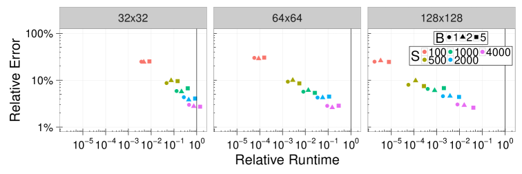
Figure 2: Relative errors $\lvert\hat{W}^{(S)}_{p}(\bm{r},\bm{s})-W_{p}(\bm{r},\bm{s})\rvert/W_{p}(\bm{r},\bm{s})$ vs. relative runtimes $\hat{t}/t$ for different parameters $S$ and $B$ and different problem sizes for images. $\hat{t}$ is the runtime of Algorithm 1 and $t$ is the runtime of the respective back-end solver without subsampling.

Figure 3: Relative errors vs. relative runtimes for different parameters $S$ and $B$ and different problem sizes for point clouds. The number of support points matches the number of pixels in the images.

As mentioned before, all results of Algorithm 1 are relative to the results of the methods applied to the original problems. We are mainly interested in the reduction in runtime and accuracy of the returned values. Many important results can be observed in Figure 2 and 3. The points in the diagram represent averages over the different methods, instances, and multiple tries, but are separated in resolution and choices of the parameters $S$ and $B$ in Algorithm 1.

For images we observe a decrease in relative runtimes with higher resolution, while the average relative error is independent of the image resolution. In the point cloud case, however, the relative error increases slightly with the instance size. The number $S$ of sampled points seems to considerably affect the relative error. An increase of the number of points results in more accurate values, with average relative errors as low as about $3\%$ for $S=4000$, while still maintaining a speedup of two orders of magnitude on $128\times 128$ images. Lower sample sizes yield higher average errors, but also lower runtimes. With $S=500$ the runtime is reduced by over four orders of magnitude with an average relative error of less than $10\%$. As to be expected, runtime increases linearly with the number of repetitions $B$. However, the impact on the relative errors is rather inconsistent. This is due to the fact, that the costs returned by the subsampling algorithm are often overestimated, therefore averaging over multiple tries does not yield improvements (see Figure 4). This means that in order to increase the accuracy of the algorithm it is advisable to keep $B=1$ and instead increase the sample size $S$. However, increasing $B$ can be useful to lower the variability of the results.

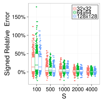
Figure 4: The signed relative approximation error $\left(\hat{W}^{(S)}_{p}(\bm{r},\bm{s})-W_{p}(\bm{r},\bm{s})\right)/W_{p}(\bm{r},\bm{s})$ showing that the approximation overestimates the exact distance for small $S$ but the bias vanishes for larger $S$.

On the contrary, there is a big difference in accuracy between the image classes. While Algorithm 1 has consistently low relative errors on the Cauchy Density images, the exact optimal costs for White Noise images cannot be approximated as reliably. The relative errors fluctuate more and are generally much higher, as one can see from Figure 5 (left). In images with smooth structures and regular features the subsamples are able to capture that structure and therefore deliver a more precise representation of the images and a more precise value. This is not possible in images that are very irregular or noisy, such as the White Noise images, which have no structure to begin with. The Classic Images contain both regular structures and more irregular regions, therefore their relative errors are slightly higher than in the Cauchy Density cases. The algorithm has a similar performance on the point cloud instances, that are modelled after the Cauchy Density and Classic Images classes, while the Dirichlet instances have a more desirable accuracy compared to the White Noise images, as seen in Figure 5 (right).

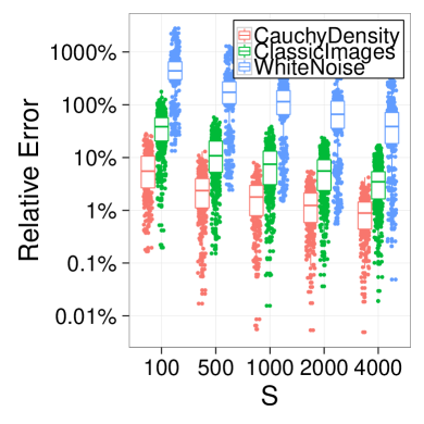
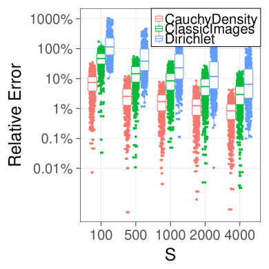
Figure 5: A comparison of the relative errors for different image classes (left) and and point cloud instance classes (right).

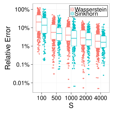
Figure 6: A comparison between the approximations of the Wasserstein and Sinkhorn distances.

There are no significant differences in performance between the different back-end solvers for the Wasserstein distance. As Figure 6 shows, accuracy seems to be better for the Sinkhorn distance compared to the other three solvers which report the exact Wasserstein distance.

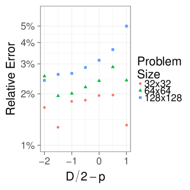
Figure 7: A comparison of the mean relative errors in the point cloud instances with sample size $S=4000$ for different values of $p^{\prime}=(\nicefrac{{D}}{{2}})-p$.

In the results of the point cloud instances we can observe the influence of the value $p^{\prime}=(\nicefrac{{D}}{{2}})-p$ on the scaling of the relative error with the instance size $N$ for constant sample size ($S=4000$). This is shown in Figure 7. We observe an increase of the relative error with $p^{\prime}$, as expected from the theory. However, we are not able to clearly distinguish between the three cases $p^{\prime}<0$, $p^{\prime}=0$ and $p^{\prime}>0$. This might be due to the relatively small instance sizes $N$ in the experiments. While we see that the relative errors are independent of $N$ in the image case (compare Figure 2), for the point clouds $N$ has an influence on the accuracy that depends on $p^{\prime}$.

5 Discussion

As our simulations demonstrate, subsampling is a simple yet powerful tool to obtain good approximations to Wasserstein distances with only a small fraction of required runtime and memory. It is especially remarkable that in the case of two dimensional images for a fixed amount of subsampled points, and therefore a fixed amount of time and memory, the relative error is independent of the resolution/size of the images. Based on these results, we expect the subsampling algorithm to return similarly precise results with even higher resolutions of the images it is applied to, while the effort to obtain them stays the same. Even in point cloud instances the relative error only scales mildly with the original input size $N$ and is dependent on the value $p^{\prime}$.

The numerical results (Figure 2) show an inverse polynomial decrease of the approximation error with $S$, in accordance with the theoretical results. In fact, the rate $\mathcal{O}(S^{-1/2p})$ is optimal. Indeed, when $\bm{r}=\bm{s}$ (are nontrivial measures), Sommerfeld and Munk (2018) show that $Z_{S}=S^{1/2p}[W_{p}(\hat{\bm{r}}_{S},\hat{\bm{s}}_{S})-W_{p}(\bm{r},\bm{s})]$ has a nondegenerate limiting distribution $Z$. For each $R>0$ the function $x\mapsto\min(R,|x|)$ is nonnegative, continuous and bounded, so

$$\liminf_{S\to\infty}E\{S^{1/2p}|W_{p}(\hat{\bm{r}}_{S},\hat{\bm{s}}_{S})-W_{p}(\bm{r},\bm{s})|\}=\liminf_{S\to\infty}E\{|Z_{S}|\}\geq\liminf_{S\to\infty}E\min\{R,|Z_{S}|\}=E\min(R,|Z|).$$

Letting $R\to\infty$ and using the monotone convergence theorem yields

$$\liminf_{S\to\infty}E\{S^{1/2p}|W_{p}(\hat{\bm{r}}_{S},\hat{\bm{s}}_{S})-W_{p}(\bm{r},\bm{s})|\}\geq E|Z|>0.$$

When applying the algorithm, it is important to note that the quality of the returned values depends on the structure of the data. In very irregular instances it is necessary to increase the sample size in order to obtain similarly precise results, while in regular structures a small sample size suffices.

Our scheme allows the parameters $S$ and $B$ to be easily tuned towards faster runtimes or more precise results, as desired. Increases and decreases of the sample size $S$ will increase/decrease the mean approximation of $W_{p}$ by $\hat{W}_{p}^{(S)}$, while $B$ will only affect the concentration around $E\hat{W}_{p}^{(S)}$. Empirically, we found that for fixed computational cost, the best performance is achieved when $B=1$ (compare Figure 2), suggesting that the bias is more dominant than the variance in the mean squared error.

The scheme presented here can readily be applied to other optimal transport distances, as long as a solver is available, as we demonstrated with the Sinkhorn distance (Cuturi, 2013). Empirically, we can report good performance in this case, suggesting that entropically regularized distances might be even more amenable to subsampling approximation than the Wasserstein distance itself. Extending the theoretical results to this case would require an analysis of the mean speed of convergence of empirical Sinkhorn distances, which is an interesting task for future research.

All in all, subsampling proves to be a general, powerful and versatile tool that can be used with virtually any optimal transport solver as back-end and has both theoretical approximation error guarantees, and a convincing performance in practice. It is a challenge to extend this method in a way which is specifically tailored to the geometry of the underlying space $\mathcal{X}$, which may result in further improvements.

Appendix

5.1 Proof of Theorem 1

Proof strategy

The method used in this proof has been employed before to bound the mean rate of convergence of the empirical Wasserstein distance on a general metric space $(\mathcal{X},d)$ (Boissard and Le Gouic, 2014; Fournier and Guillin, 2015). In essence, it constructs a tree on the space $\mathcal{X}$ and bounds the Wasserstein distance with some transport metric in the tree, which can either be computed explicitly or bounded easily (see also Heinrich and Kahn (2018), who use a coarse-graining tree in order to bound the Wasserstein distance in the context of mixture models). Our construction is specifically tailored to finite spaces, and allows to obtain a better dependence on $N=|\mathcal{X}|$ in Theorem 3 while preserving the rate $S^{-1/2}$.

More precisely, in our case of finite spaces, let $\mathcal{T}$ be a spanning tree on $\mathcal{X}$ (that is, a tree with vertex set $\mathcal{X}$ and edge lengths given by the metric $d$ on $\mathcal{X}$) and $d_{\mathcal{T}}$ the metric on $\mathcal{X}$ defined by the path lengths in the tree. Clearly, the tree metric $d_{\mathcal{T}}$ dominates the original metric $d$ on $\mathcal{X}$ and hence $W_{p}(\bm{r},\bm{s})\leq W_{p}^{\mathcal{T}}(\bm{r},\bm{s})$ for all $\bm{r},\bm{s}\in\mathcal{P}(\mathcal{X})$, where $W_{p}^{\mathcal{T}}$ denotes the Wasserstein distance evaluated with respect to the tree metric. The goal is now to bound $E\left[(W_{p}^{\mathcal{T}}(\hat{\bm{r}}_{S},\bm{r}))^{p}\right]$. We refer to Tameling and Munk (2018) for examples and comparisons of different spanning trees on two-dimensional grids.

Assume $\mathcal{T}$ is rooted at $\mathrm{root}(\mathcal{T})\in\mathcal{X}$. Then, for $x\in\mathcal{X}$ and $x\neq\mathrm{root}(\mathcal{T})$ we may define $\mathrm{par}(x)\in\mathcal{X}$ as the immediate neighbor of $x$ in the unique path connecting $x$ and $\mathrm{root}(\mathcal{T})$. We set $\mathrm{par}(\mathrm{root}(\mathcal{T}))=\mathrm{root}(\mathcal{T})$. We also define $\mathrm{children}(x)$ as the set of vertices $x^{\prime}\in\mathcal{X}$ such that there exists a sequence $x^{\prime}=x_{1},\dots,x_{l}=x\in\mathcal{X}$ with $\mathrm{par}(x_{j})=x_{j+1}$ for $j=1,\dots,l-1$. Note that with this definition $x\in\mathrm{children}(x)$. Additionally, define the linear operator $S_{\mathcal{T}}\colon\mathbb{R}^{\mathcal{X}}\rightarrow\mathbb{R}^{\mathcal{X}}$

$$(S_{\mathcal{T}}{\bm{u}})_{x}=\sum_{x^{\prime}\in\mathrm{children}(x)}u_{x^{\prime}}.$$ (10)

Building the tree

We build a $q$-ary tree on $\mathcal{X}$. To this end, we split $\mathcal{X}$ to $l_{\max}+2$ groups and build the tree in such a way that a node at level $l+1$ has a unique parent at level $l$ with edge length $q^{-l}$. The formal construction follows.

For $l\in\{0,\dots,l_{\max}\}$ we let $Q_{l}\subset\mathcal{X}$ be the center points of a $q^{-l}\>\mathrm{diam}(\mathcal{X})$ covering of $\mathcal{X}$, that is

$$\bigcup_{x\in Q_{l}}B(x,q^{-l}\>\mathrm{diam}(\mathcal{X}))=\mathcal{X},\text{ and }|Q_{l}|=\mathcal{N}(\mathcal{X},q^{-l}\>\mathrm{diam}(\mathcal{X})),$$

where $B(x,\epsilon)=\{x^{\prime}\in\mathcal{X}:d(x,x^{\prime})\leq\epsilon\}$. Additionally set $Q_{l_{\max}+1}=\mathcal{X}$. Now define $\tilde{Q}_{l}=Q_{l}\times\{l\}$ and we will build a tree structure on $\cup_{l=0}^{l_{\max}+1}\tilde{Q}_{l}$.

Since we must have $|\tilde{Q}_{0}|=1$ we can take this element as the root. Assume now that the tree already contains all elements of $\cup_{j=0}^{l}\tilde{Q}_{j}$. Then, we add to the tree all elements of $\tilde{Q}_{l+1}$ by choosing for $(x,l+1)\in\tilde{Q}_{l+1}$ (exactly one) parent element $(x^{\prime},l)\in\tilde{Q}_{l}$ such that $d(x,x^{\prime})\leq q^{-l}\>\mathrm{diam}(\mathcal{X})$. This is possible, since $Q_{l}$ is a $q^{-l}\>\mathrm{diam}(\mathcal{X})$ covering of $\mathcal{X}$. We set the length of the connecting edge to $q^{-l}\>\mathrm{diam}(\mathcal{X})$.

In this fashion we obtain a spanning tree $\mathcal{T}$ of $\cup_{l=0}^{l_{\max}+1}\tilde{Q}_{l}$ and a partition $\{\tilde{Q}_{l}\}_{l=0,\dots,l_{\max}+1}$. About this tree we know that

• it is in fact a tree. First, it is connected, because the construction starts with one connected component and in every subsequent step all additional vertices are connected to it. Second, it contains no cycles. To see this let $((x_{1},l_{1}),\dots,(x_{K},l_{K}))$ be a cycle in $\mathcal{T}$. Without loss of generality we may assume $l_{1}=\min\{l_{1},\dots,l_{K}\}$. Then, $(x_{1},l_{1})$ must have at least two edges connecting it to vertices in a $\tilde{Q}_{l}$ with $l\geq l_{1}$ which is impossible by construction.

• $|\tilde{Q}_{l}|=\mathcal{N}(\mathcal{X},q^{-l}\>\mathrm{diam}(\mathcal{X}))$ for $0\leq l\leq l_{\max}$.

• $d(x,\mathrm{par}(x))=q^{-l+1}\>\mathrm{diam}(\mathcal{X})$ whenever $x\in\tilde{Q}_{l}$, $l\geq 1$.

• $d(x,x^{\prime})\leq d_{\mathcal{T}}\left((x,l_{\max}+1),(x^{\prime},l_{\max}+1)\right)$.

Since the leaves of $\mathcal{T}$ can be identified with $\mathcal{X}$ a measure $\bm{r}\in\mathcal{P}(\mathcal{X})$ canonically defines a probability measure $\bm{r}^{\mathcal{T}}\in\mathcal{P}(\mathcal{T})$ for which $r^{\mathcal{T}}_{(x,l_{\max}+1)}=r_{x}$ and $r^{\mathcal{T}}_{(x,l)}=0$ for $l\leq l_{\max}$. In slight abuse of notation we will denote the measure $\bm{r}^{\mathcal{T}}$ simply by $\bm{r}$. With this notation, we have $W_{p}(\bm{r},\bm{s})\leq W_{p}^{\mathcal{T}}(\bm{r},\bm{s})$ for all $\bm{r},\bm{s}\in\mathcal{P}(\mathcal{X})$.

Wasserstein distance on trees

Note also that $\mathcal{T}$ is ultra-metric that is, all its leaves are at the same distance from the root. For trees of this type, we can define a height function $h:\mathcal{X}\rightarrow[0,\infty)$ such that $h(x)=0$ if $x\in\mathcal{X}$ is a leaf and $h(\mathrm{par}(x))-h(x)=d_{\mathcal{T}}(x,\mathrm{par}(x))$ for all $x\in\mathcal{X}\setminus\mathrm{root}(\mathcal{X})$. There is an explicit formula for the Wasserstein distance on ultra-metric trees (Kloeckner, 2015). Indeed, if $\bm{r},\bm{s}\in\mathcal{P}(\mathcal{X})$ then

$$(W_{p}^{\mathcal{T}}(\bm{r},\bm{s}))^{p}=2^{p-1}\sum_{x\in\mathcal{X}}\left(h(\mathrm{par}(x))^{p}-h(x)^{p}\right)\left|(S_{\mathcal{T}}\bm{r})_{x}-(S_{\mathcal{T}}\bm{s})_{x}\right|,$$ (11)

with the operator $S_{\mathcal{T}}$ as defined in (10). For the tree $\mathcal{T}$ constructed above and $x\in\tilde{Q}_{l}$ with $l=0,\dots,l_{\max}$ we have

$$h(x)=\sum_{j=l}^{l_{\max}}q^{-j}\>\mathrm{diam}(\mathcal{X}),$$

and therefore $\>\mathrm{diam}(\mathcal{X})q^{-l}\leq h(x)\leq 2\>\mathrm{diam}(\mathcal{X})q^{-l}$. This yields

$$(h(\mathrm{par}(x))^{p}-(h(x))^{p})\leq(\>\mathrm{diam}(\mathcal{X}))^{p}q^{-(l-2)p}.$$

Then (11) yields

$$E\left[W_{p}^{p}(\hat{\bm{r}}_{S},\bm{r})\right]\leq 2^{p-1}q^{2p}(\>\mathrm{diam}(\mathcal{X}))^{p}\sum_{l=0}^{l_{\max}+1}q^{-lp}\sum_{x\in\tilde{Q}_{l}}E|(S_{\mathcal{T}}\hat{\bm{r}}_{S})_{x}-(S_{\mathcal{T}}\bm{r})_{x}|.$$

Since $(S_{\mathcal{T}}\hat{\bm{r}}_{S})_{x}$ is the mean of $S$ i.i.d. Bernoulli variables with expectation $(S_{\mathcal{T}}\bm{r})_{x}$ we have

$$\sum_{x\in\tilde{Q}_{l}}E|(S_{\mathcal{T}}\hat{\bm{r}}_{S})_{x}-(S_{\mathcal{T}}\bm{r})_{x}|\leq\sum_{x\in\tilde{Q}_{l}}\sqrt{\frac{(S_{\mathcal{T}}\bm{r})_{x}(1-(S_{\mathcal{T}}\bm{r})_{x})}{S}}\\ \leq\frac{1}{\sqrt{S}}\left(\sum_{x\in\tilde{Q}_{l}}(S_{\mathcal{T}}\bm{r})_{x}\right)^{1/2}\left(\sum_{x\in\tilde{Q}_{l}}(1-(S_{\mathcal{T}}\bm{r})_{x})\right)^{1/2}\leq\sqrt{|\tilde{Q}_{l}|/S},$$

using Hölder’s inequality and the fact that $\sum_{x\in\tilde{Q}_{l}}(S_{\mathcal{T}}\bm{r})_{x}=1$ for all $l=0,\dots,l_{\max}+1$. This finally yields

$$E\left[W_{p}^{p}(\hat{\bm{r}}_{S},\bm{r})\right]\leq 2^{p-1}q^{2p}(\>\mathrm{diam}(\mathcal{X}))^{p}\left(q^{-(l_{\max}+1)p}\sqrt{N}+\sum_{l=0}^{l_{\max}}q^{-lp}\sqrt{\mathcal{N}(\mathcal{X},q^{-l}\>\mathrm{diam}(\mathcal{X}))}\right)/\sqrt{S}\\ \leq\mathcal{E}_{q}(\mathcal{X},p)/\sqrt{S}.$$

Covering by arbitrary sets

We now explain how to obtain the second formula for $\mathcal{E}_{q}$ as stated in Remark 2. The idea is to define the coverings with arbitrary sets, not necessarily balls. Let

$$\mathcal{N}_{1}(\mathcal{X},\delta)=\inf\{m:\exists A_{1},\dots,A_{m}\subseteq\mathcal{X},\>\mathrm{diam}(A_{i})\leq 2\delta,\cup A_{i}\supseteq\mathcal{X}\}.$$

Since balls satisfy the diameter condition, $\mathcal{N}_{1}\leq\mathcal{N}$. Furthermore, if $\mathcal{X}^{\prime}\supseteq\mathcal{X}$, then $\mathcal{N}_{1}(\mathcal{X},\delta)\leq\mathcal{N}_{1}(\mathcal{X}^{\prime},\delta)$, which is not the case for $\mathcal{N}$. For example, let $\mathcal{X}=\{-1,1\}\subset\{-1,0,1\}=\mathcal{X}^{\prime}$ and observe that

$$\mathcal{N}_{1}(\mathcal{X},1)=1=\mathcal{N}_{1}(\mathcal{X}^{\prime},1),\qquad\textrm{but}\qquad\mathcal{N}(\mathcal{X},1)=2>1=\mathcal{N}(\mathcal{X}^{\prime},1).$$

The tree construction with respect to the new covering numbers is done in a similar manner. For each $0\leq l\leq l_{\max}$ let $Q_{l}^{\prime}$ be a collection of disjoint sets of diameter $2q^{-l}\>\mathrm{diam}(\mathcal{X})$ that cover $\mathcal{X}$ and $|Q_{l}^{\prime}|=\mathcal{N}_{1}(\mathcal{X},q^{-l}\>\mathrm{diam}(\mathcal{X}))$. Let $Q_{l}=\{x_{1},\dots,x_{|Q_{l}^{\prime}|}\}\subseteq\mathcal{X}$ be an arbitrary collection of representatives from the sets in $Q_{l}^{\prime}$. Such representatives exist by minimality of $|Q_{l}^{\prime}|$ and they are different by the disjoint nature of $Q_{l}^{\prime}$. Additionally set $Q_{l_{\max}+1}=\mathcal{X}$. Construct the tree in the same way, except that now we only have the bound $d(x,x^{\prime})\leq 2q^{-l}\>\mathrm{diam}(\mathcal{X})$ for $(x,l+1)\in\tilde{Q}_{l+1}$ and a corresponding $(x,l)\in\tilde{Q}_{l}$, so we need to set the edge length to be $2q^{-l}\>\mathrm{diam}(\mathcal{X})$, twice as much as in the original construction. The proof then goes in the same way, with an extra factor $2^{p}$. We obtain an alternative bound

$$\mathcal{E}_{q}=2^{2p-1}q^{2p}(\>\mathrm{diam}(\mathcal{X}))^{p}\left(q^{-(l_{\max}+1)p}\sqrt{N}+\sum_{l=0}^{l_{\max}}q^{-lp}\sqrt{\mathcal{N}_{1}(\mathcal{X},q^{-l}\>\mathrm{diam}(\mathcal{X}))}\right).$$

In comparison with (6), we replaced $\mathcal{N}$ by $\mathcal{N}_{1}$. The price to pay for this is an additional factor of $2^{p}$.

5.2 Proof of Theorem 3

We may assume without loss of generality that $\mathcal{X}\subseteq[0,\>\mathrm{diam}(\mathcal{X})]^{D}$. The covering numbers of the cube with Euclidean balls behave badly in high dimensions, so it will prove useful to replace the Euclidean norm by the infinity norm $\|x\|_{\infty}=\max_{i}|x_{i}|$, $x=(x_{1},\dots,x_{D})\in\mathbb{R}^{D}$. With this norm we have $\mathcal{N}([0,\>\mathrm{diam}(\mathcal{X})]^{D},\epsilon\>\mathrm{diam}(\mathcal{X}),\|\cdot\|_{\infty})\leq(\lceil 1/(2\epsilon)\rceil)^{D}$. If $q$ is an integer, then

$$\mathcal{N}(\mathcal{X},q^{-l}\>\mathrm{diam}(\mathcal{X}),\|\cdot\|_{\infty})\leq\mathcal{N}([0,\>\mathrm{diam}(\mathcal{X})]^{D},q^{-l}\>\mathrm{diam}(\mathcal{X})/2,\|\cdot\|_{\infty})\leq\lceil q^{l}\rceil^{D}=q^{lD}.$$

This yields

$$\sum_{l=0}^{l_{\max}}q^{-lp}\sqrt{\mathcal{N}(\mathcal{X},q^{-l}\>\mathrm{diam}(\mathcal{X}))}\leq\sum_{l=0}^{l_{\max}}q^{l(D/2-p)}=\begin{cases}(1-q^{(l_{\max}+1)(D/2-p)})/(1-q^{D/2-p})&\text{if }D\neq 2p,\\ l_{\max}+1&\text{if }D=2p.\end{cases}$$

Denote for brevity $p^{\prime}=D/2-p$ and plug this into (6):

$$S^{1/2}E\left[W_{p}^{p}(\hat{\bm{r}}_{S},\bm{r},\|\cdot\|_{\infty})\right]\leq 2^{p-1}q^{2p}(\>\mathrm{diam}(\mathcal{X}))^{p}\left[q^{-p(l_{\max}+1)}\sqrt{N}+\begin{cases}(1-q^{(l_{\max}+1)p^{\prime}})/(1-q^{p^{\prime}})&\text{if }p^{\prime}\neq 0,\\ l_{\max}+1&\text{if }p^{\prime}=0.\end{cases}\right]$$

If $p^{\prime}<0$, then let $l_{\max}\to\infty$. Otherwise, choose $l_{\max}=\lfloor D^{-1}\log_{q}N\rfloor$ (giving the best dependence on $N$), so that the element inside the square brackets is smaller than

$$\begin{cases}1/(1-q^{p^{\prime}})&\text{if }p^{\prime}<0,\\ 2+D^{-1}\log_{q}N&\text{if }p^{\prime}=0,\\ N^{1/2-p/D}+(N^{1/2-p/D}q^{p^{\prime}}-1)/(q^{p^{\prime}}-1)&\text{if }p^{\prime}>0\end{cases}\quad\leq\quad\begin{cases}1/(1-q^{p^{\prime}})&\text{if }p^{\prime}<0,\\ 2+D^{-1}\log_{q}N&\text{if }p^{\prime}=0,\\ (2q^{p^{\prime}}-1)N^{1/2-p/D}/(q^{p^{\prime}}-1)&\text{if }p^{\prime}>0.\end{cases}$$ (12)

The right-hand side is $C_{D,p}(N)$ for $q=2$. To get back to the Euclidean norm use $\|a\|_{2}\leq\|a\|_{\infty}\sqrt{D}$, so that

$$E\left[W_{p}^{p}(\hat{\bm{r}}_{S},\bm{r})\right]\leq D^{p/2}E\left[W_{p}^{p}(\hat{\bm{r}}_{S},\bm{r},\|\cdot\|_{\infty})\right]\leq D^{p/2}2^{p-1}q^{2p}(\>\mathrm{diam}(\mathcal{X}))^{p}C_{D,p}(N)/\sqrt{S},$$

which is the desired conclusion.

Lemma 1.

1. Let $\tilde{C}_{D,p}(q,N)$ denote the right-hand side of (12). Then the minimum of the function $q\mapsto q^{2p}\tilde{C}_{D,p}(q,N)$ on $[2,\infty)$ is attained at $q=2$.

2. Let $q\geq 2$, $p,D$ integers, and $p^{\prime}=D/2-p$. If $p^{\prime}<0$, then $1/(1-q^{p^{\prime}})\leq 2+\sqrt{2}$ and if $p^{\prime}>0$, then $2+1/(q^{p^{\prime}}-1)\leq 3+\sqrt{2}$.

Proof.

We begin with (b). If $p^{\prime}<0$ then $1/(1-q^{p^{\prime}})$ is decreasing in $q$ and increasing in $p^{\prime}$. The integer constaints on $D$ and $p$ imply that the maximal value $p^{\prime}$ can attain is $-0.5$. The smaller value $q$ can attain is 2. Thus

$$1/(1-q^{p^{\prime}})\leq 1/(1-2^{-0.5})=\frac{\sqrt{2}}{\sqrt{2}-1}=\sqrt{2}(\sqrt{2}+1)=2+\sqrt{2}.$$

When $p^{\prime}>0$ the term $2+1/(q^{p^{\prime}}-1)$ is decreasing in $p^{\prime}\geq 0.5$ and in $q\geq 2$, so it is bounded by

$$2+1/(\sqrt{2}-1)=3+\sqrt{2}.$$

To prove (a) we shall differentiate the function $q^{2p}\tilde{C}_{D,p}(q,N)$ with respect to $q$ and show that the derivative is positive for all $q\geq 2$, and $p,D,N\geq 1$.

For negative $p^{\prime}$ consider the function

$$f_{1}(q)=\frac{q^{2p}}{1-q^{p^{\prime}}},\qquad q\geq 2;p\geq 1;p^{\prime}<0.$$

Its derivative is

$$f_{1}^{\prime}(q)=\frac{2pq^{2p-1}(1-q^{p^{\prime}})+p^{\prime}q^{p^{\prime}-1}q^{2p}}{(1-q^{p^{\prime}})^{2}}=\frac{q^{2p-1}}{1-q^{p^{\prime}}}\left[2p+\frac{p^{\prime}q^{p^{\prime}}}{1-q^{p^{\prime}}}\right].$$

It suffices to show that the term in square brackets is positive, since $1-q^{p^{\prime}}>0$. Let us bound $q^{p^{\prime}}$ and the denominator $(1-q^{p^{\prime}})^{-1}$. Since $e^{x}\geq 1+x$ for $x\geq 0$, $e^{-x}\leq 1/(1+x)$ and setting $x=-p^{\prime}\log q$ gives

$$q^{p^{\prime}}=e^{p^{\prime}\log q}\leq\frac{1}{1-p^{\prime}\log q}.$$

Hence

$$1-q^{p^{\prime}}\geq 1-\frac{1}{1-p^{\prime}\log q}=\frac{1-p^{\prime}\log q-1}{1-p^{\prime}\log q}=\frac{-p^{\prime}\log q}{1-p^{\prime}\log q}.$$

so that

$$\frac{q^{p^{\prime}}}{1-q^{p^{\prime}}}\leq\frac{1}{1-p^{\prime}\log q}\frac{1-p^{\prime}\log q}{-p^{\prime}\log q}=\frac{1}{-p^{\prime}\log q}.$$

Conclude that, since $p^{\prime}<0$,

$$2p+\frac{p^{\prime}q^{p^{\prime}}}{1-q^{p^{\prime}}}\geq 2p+p^{\prime}\frac{1}{-p^{\prime}\log q}=2p+\frac{1}{-\log q}=2p-\frac{1}{\log q}\geq 2p-\frac{1}{\log 2}\geq 2-\frac{1}{\log 2}>0.$$

For $p^{\prime}=0$ consider the function

$$f_{2}(q)=q^{2p}(2+D^{-1}\log_{q}N)=2q^{2p}+\frac{q^{2p}\log N}{D\log q},\qquad q\geq 2;D=2p\geq 2.$$

Its derivative is

$$f_{2}^{\prime}(q)=4pq^{2p-1}+\frac{\log N}{D(\log q)^{2}}\left[2pq^{2p-1}\log q-q^{-1}q^{2p}\right]=q^{2p-1}\left[4p+\frac{\log N}{D(\log q)^{2}}(2p\log q-1)\right]>0$$

since $2p\log q\geq 2\log 2>1$.

For $p^{\prime}>0$ consider the function

$$f_{3}(q)=q^{2p}[2+1/(q^{p^{\prime}}-1)]=2q^{2p}+\frac{q^{2p}}{q^{p^{\prime}}-1}=2q^{2p}-f_{1}(q),\qquad q\geq 2;p\geq 1;p^{\prime}>0.$$

The derivative is

$$4pq^{2p-1}-\frac{q^{2p-1}}{1-q^{p^{\prime}}}\left[2p+\frac{p^{\prime}q^{p^{\prime}}}{1-q^{p^{\prime}}}\right]=4pq^{2p-1}+\frac{q^{2p-1}}{q^{p^{\prime}}-1}\left[2p-\frac{p^{\prime}q^{p^{\prime}}}{q^{p^{\prime}}-1}\right].$$

This function is more complicated and we need to split into cases according to small, large or moderate values of $p^{\prime}$.

Case 1: $p^{\prime}\leq 0.5$. Then the negative term can be bounded using $q^{p^{\prime}}-1\geq p^{\prime}\log q$ as

$$\frac{p^{\prime}q^{p^{\prime}}}{q^{p^{\prime}}-1}=p^{\prime}+\frac{p^{\prime}}{q^{p^{\prime}}-1}\leq p^{\prime}+\frac{1}{\log q}\leq p^{\prime}+\frac{1}{\log 2}\leq 0.5+\frac{1}{\log 2}<2\leq 2p.$$

Thus $f_{3}^{\prime}(q)\geq 0$ in this case.

To deal with larger values of $p^{\prime}$ rewrite the derivative as

$$q^{2p-1}\left[4p+\frac{2p}{q^{p^{\prime}}-1}-\frac{p^{\prime}q^{p^{\prime}}}{(q^{p^{\prime}}-1)^{2}}\right],$$

and bound the negative part:

$$\frac{p^{\prime}q^{p^{\prime}}}{(q^{p^{\prime}}-1)^{2}}=\frac{p^{\prime}}{q^{p^{\prime}}-1}+\frac{p^{\prime}}{(q^{p^{\prime}}-1)^{2}}\leq\frac{1}{\log q}+\frac{1}{(q^{p^{\prime}}-1)\log q}.$$

Case 2: $p^{\prime}\geq 1$. Then $q^{p^{\prime}}-1\geq 1$ so this is smaller than

$$\frac{1}{\log 2}+\frac{1}{\log 2}=\frac{2}{\log 2}<4\leq 4p.$$

Hence the derivative is positive in this case.

Case 3: $p^{\prime}\geq 1/2$ and $q\geq e$. Then this is smaller than

$$1+\frac{1}{e^{1/2}-1}\leq 1+\frac{1}{\sqrt{2}-1}=2+\sqrt{2}<4\leq 4p.$$

Hence the derivative is positive in this case.

Case 4: $q\leq e$ and $p^{\prime}\in[1/2,1]$. The negative term is bounded by

$$\frac{1}{\log q}+\frac{1}{(q^{p^{\prime}}-1)\log q}\leq\frac{1}{\log 2}+\frac{1}{(q^{p^{\prime}}-1)\log 2}\leq\frac{1}{\log 2}+\frac{1}{(\sqrt{2}-1)\log 2}=\frac{2+\sqrt{2}}{\log 2}\approx 4.93,$$

whereas the positive term can be bounded below as

$$4p+\frac{2p}{q^{p^{\prime}}-1}\geq 4+\frac{2}{e-1}\approx 5.16>4.93.$$

This completes the proof.

∎

5.3 Proof of Theorem 4

We introduce some additional notation. For $(x,y),(x^{\prime},y^{\prime})\in\mathcal{X}^{2}$ we set

$$d_{\mathcal{X}^{2}}((x,y),(x^{\prime},y^{\prime}))=\left\{d^{p}(x,x^{\prime})+d^{p}(y,y^{\prime})\right\}^{1/p}$$

We further define the function $Z:(\mathcal{X}^{2})^{SB}\rightarrow\mathbb{R}$ via

$$\begin{split}\left((x_{11},y_{11}),\dots,(x_{SB},y_{SB})\right)\mapsto\frac{1}{B}\sum_{i=1}^{B}\left[W_{p}\left(\frac{1}{S}\sum_{j=1}^{S}\delta_{x_{ji}},\frac{1}{S}\sum_{j=1}^{S}\delta_{y_{ji}}\right)-W_{p}(\bm{r},\bm{s})\right].\end{split}$$

Since $W_{p}^{p}(\cdot,\cdot)$ is jointly convex (Villani, 2008, Theorem 4.8),

$$W_{p}\left(\frac{1}{S}\sum_{j=1}^{S}\delta_{x_{j}},\frac{1}{S}\sum_{j=1}^{S}\delta_{y_{j}}\right)\leq\left\{\frac{1}{S}\sum_{j=1}^{S}W_{p}^{p}(\delta_{x_{j}},\delta_{y_{j}})\right\}^{1/p}=S^{-1/p}\left\{\sum_{j=1}^{S}d^{p}(x_{j},y_{j})\right\}^{1/p}.$$

Our first goal is to show that $Z$ is Lipschitz continuous. To this end, let $((x_{11},y_{11}),\dots,(x_{SB},y_{SB}))$ and $((x^{\prime}_{11},y^{\prime}_{11}),\dots,(x^{\prime}_{SB},y^{\prime}_{SB}))$ arbitrary elements of $(\mathcal{X}^{2})^{SB}$. Then, using the reverse triangle inequality and the relations above

$$|Z((x_{11},y_{11}),\dots,(x_{SB},y_{SB}))-Z((x^{\prime}_{11},y^{\prime}_{11}),\dots,(x^{\prime}_{SB},y^{\prime}_{SB}))|$$

$$\leq\frac{1}{B}\sum_{i=1}^{B}\bigg{|}W_{p}\left(\frac{1}{S}\sum_{j=1}^{S}\delta_{x_{ji}},\frac{1}{S}\sum_{j=1}^{S}\delta_{y_{ji}}\right)-W_{p}\left(\frac{1}{S}\sum_{j=1}^{S}\delta_{x^{\prime}_{ji}},\frac{1}{S}\sum_{j=1}^{S}\delta_{y^{\prime}_{ji}}\right)\bigg{|}$$

$$\leq\frac{1}{B}\sum_{i=1}^{B}\bigg{[}W_{p}\left(\frac{1}{S}\sum_{j=1}^{S}\delta_{x_{ji}},\frac{1}{S}\sum_{j=1}^{S}\delta_{x^{\prime}_{ji}}\right)+W_{p}\left(\frac{1}{S}\sum_{j=1}^{S}\delta_{y_{ji}},\frac{1}{S}\sum_{j=1}^{S}\delta_{y^{\prime}_{ji}}\right)\bigg{]}$$

$$\leq\frac{S^{-1/p}}{B}\sum_{i=1}^{B}\bigg{[}\left\{\sum_{j=1}^{S}d^{p}(x_{ji},x^{\prime}_{ji})\right\}^{1/p}+\left\{\sum_{j=1}^{S}d^{p}(y_{ji},y^{\prime}_{ji})\right\}^{1/p}\bigg{]}$$

$$\leq\frac{S^{-1/p}}{B}\left(2B\right)^{\frac{p-1}{p}}\left\{\sum_{i,j}d^{p}_{\mathcal{X}^{2}}((x_{ji},y_{ji}),(x^{\prime}_{ji},y^{\prime}_{ji}))\right\}^{1/p}$$

Hence, $Z/2$ is Lipschitz continuous with constant $(SB)^{-1/p}$ relative to the $p$-metric generated by $d_{\mathcal{X}^{2}}$ on $(\mathcal{X}^{2})^{SB}$.

For $\tilde{\bm{r}}\in\mathcal{P}({\mathcal{X}^{2}})$ let $H(\cdot\>|\>\tilde{\bm{r}})$ denote the relative entropy with respect to $\tilde{\bm{r}}$. Since $\mathcal{X}^{2}$ has $d_{\mathcal{X}^{2}}$-diameter $2^{1/p}\>\mathrm{diam}(\mathcal{X})$, we have by Bolley and Villani (2005, Particular case $2.5$, page $337$) that for every $\tilde{\bm{s}}$

$$W_{p}(\tilde{\bm{r}},\tilde{\bm{s}})\leq\left(8\>\mathrm{diam}(\mathcal{X})^{2p}H(\tilde{\bm{r}}\>|\>\tilde{\bm{s}})\right)^{1/2p}.$$ (13)

If $X_{11},\dots,X_{SB}\sim\bm{r}$ and $Y_{11},\dots,Y_{SB}\sim\bm{s}$ are all independent, we have

$$Z((X_{11},Y_{11}),\dots,(X_{SB},Y_{SB}))\sim\hat{W}^{(S)}_{p}(\bm{r},\bm{s})-W_{p}(\bm{r},\bm{s}).$$

The Lipschitz continuity of $Z$ and the transportation inequality (13) yields a concentration result for this random variable. In fact, by Gozlan and Léonard (2007, Lemma 6) we have

$$P\bigg{[}\hat{W}^{(S)}_{p}(\bm{r},\bm{s})-W_{p}(\bm{r},\bm{s})\geq E\left[\hat{W}^{(S)}_{p}(\bm{r},\bm{s})-W_{p}(\bm{r},\bm{s})\right]+z\bigg{]}\leq\exp\left(\frac{-SBz^{2p}}{8\>\>\mathrm{diam}(\mathcal{X})^{2p}}\right).$$

for all $z\geq 0$. Note that $-Z$ is Lipschitz continuous as well and hence, by the union bound,

$$P\bigg{[}\left|\hat{W}^{(S)}_{p}(\bm{r},\bm{s})-W_{p}(\bm{r},\bm{s})\right|\geq E\left[\left|\hat{W}^{(S)}_{p}(\bm{r},\bm{s})-W_{p}(\bm{r},\bm{s})\right|\bigg{]}+z\right]\leq 2\exp\left(\frac{-SBz^{2p}}{8\>\>\mathrm{diam}(\mathcal{X})^{2p}}\right).$$

Now, with the reverse triangle inequality, Jensen’s inequality and Theorem 1,

$$E\left[\left|\hat{W}^{(S)}_{p}(\bm{r},\bm{s})-W_{p}(\bm{r},\bm{s})\right|\right]\leq E\left[W_{p}(\hat{\bm{r}}_{S},\bm{r})+W_{p}(\hat{\bm{s}}_{S},\bm{s})\right]\\ \leq E\left[W_{p}^{p}(\hat{\bm{r}}_{S},\bm{r})\right]^{1/p}+\left[W_{p}^{p}(\hat{\bm{s}}_{S},\bm{s})\right]^{1/p}\leq 2\mathcal{E}_{q}^{1/p}/S^{1/(2p)}.$$

Together with the last concentration inequality above, this concludes the proof of Theorem 4.

5.4 Proof of Theorem 5

Denote $V=|\hat{W}^{(S)}_{p}(\bm{r},\bm{s})-W_{p}(\bm{r},\bm{s})|$, $C=2\mathcal{E}_{q}^{1/p}/S^{1/(2p)}\geq 0$, and observe that

$$E\left[V^{2}\right] =\int_{0}^{\infty}P(V>\sqrt{t})dt=2\int_{0}^{\infty}P(V>s)sds=2\int_{-C}^{\infty}P(V>z+C)(z+C)dz$$

$$\leq 2\int_{-C}^{C}(z+C)dz+4\int_{C}^{\infty}P(V>z+C)zdz\leq 4C^{2}+8\int_{C}^{\infty}z\exp\left(-\frac{SBz^{2p}}{8\>\>\mathrm{diam}(\mathcal{X})^{2p}}\right)dz$$

by Theorem 4. Changing variables and using the inequality $y^{2p}\geq y^{2}$ (valid for $y,p\geq 1)$ gives

$$8\int_{C}^{\infty}z\exp\left(-\frac{SBz^{2p}}{8\>\>\mathrm{diam}(\mathcal{X})^{2p}}\right)dz =8C^{2}\int_{1}^{\infty}y\exp\left(-\frac{SB(Cy)^{2p}}{8\>\>\mathrm{diam}(\mathcal{X})^{2p}}\right)dy$$

$$\leq 8C^{2}\int_{1}^{\infty}y\exp\left(-\frac{SBC^{2p}y^{2}}{8\>\>\mathrm{diam}(\mathcal{X})^{2p}}\right)dy =8C^{2}\frac{4(\>\mathrm{diam}(\mathcal{X}))^{2p}}{SBC^{2p}}\exp\left(-\frac{SBC^{2p}}{8\>\>\mathrm{diam}(\mathcal{X})^{2p}}\right)$$

$$=4C^{2}\frac{(\>\mathrm{diam}(\mathcal{X}))^{2p}}{2^{2p-3}\mathcal{E}_{q}^{2}B}\exp\left(-\frac{4^{p}\mathcal{E}_{q}^{2}B}{8\>\>\mathrm{diam}(\mathcal{X})^{2p}}\right),$$

where we have used $C^{2}=4\mathcal{E}_{q}^{2/p}S^{-1/p}$. Deduce that

$$E\left[\left|\hat{W}^{(S)}_{p}(\bm{r},\bm{s})-W_{p}(\bm{r},\bm{s})\right|^{2}\right]\leq 16\mathcal{E}_{q}^{2/p}\left\{1+\frac{(\>\mathrm{diam}(\mathcal{X}))^{2p}}{2^{2p-3}\mathcal{E}_{q}^{2}B}\exp\left(-\frac{4^{p}\mathcal{E}_{q}^{2}B}{8\>\>\mathrm{diam}(\mathcal{X})^{2p}}\right)\right\}S^{-1/p}\leq 18\mathcal{E}_{q}^{2/p}S^{-1/p}.$$

For the last inequality, note that (6) implies $\mathcal{E}_{q}^{2}\geq 2^{6p-2}[\>\mathrm{diam}(\mathcal{X})]^{2p}$ and hence $[\>\mathrm{diam}(\mathcal{X})]^{2p}/[B2^{2p-3}\mathcal{E}_{q}^{2}]\leq 2^{5-8p}\leq 1/8$, so the term in parentheses is smaller than $1+1/8$.

Similar computations show that $E\left[\left|\hat{W}^{(S)}_{p}(\bm{r},\bm{s})-W_{p}(\bm{r},\bm{s})\right|^{\alpha}\right]=\mathcal{O}(S^{-\alpha/(2p)})$ for all $0\leq\alpha\leq 2p$.

References

• Agueh and Carlier (2011) Martial Agueh and Guillaume Carlier. Barycenters in the Wasserstein space. SIAM J. Math. Anal., 43(2):904–924, 2011.
• Altschuler et al. (2017) Jason Altschuler, Jonathan Weed, and Philippe Rigollet. Near-linear time approximation algorithms for optimal transport via Sinkhorn iteration. In I Guyon, U V Luxburg, S Bengio, H Wallach, R Fergus, S Vishwanathan, and R Garnett, editors, Advances in Neural Information Processing Systems, pages 1964–1974, Red Hook, NY, 2017. Curran.
• Bertsekas (1992) Dimitri P. Bertsekas. Auction algorithms for network flow problems: A tutorial introduction. Computational Optimization and Applications, 1(1):7–66, 1992.
• Boissard and Le Gouic (2014) Emmanuel Boissard and Thibaut Le Gouic. On the mean speed of convergence of empirical and occupation measures in Wasserstein distance. Ann. Inst. H. Poincaré Probab. Statist., 50(2):539–563, 2014.
• Bolley and Villani (2005) François Bolley and Cédric Villani. Weighted Csiszár-Kullback-Pinsker inequalities and applications to transportation inequalities. Annales de La Faculté Des Sciences de Toulouse: Mathématiques, 14(3):331–352, 2005.
• Bonneel et al. (2015) Nicolas Bonneel, Julien Rabin, Gabriel Peyré, and Hanspeter Pfister. Sliced and Radon Wasserstein barycenters of measures. Journal of Mathematical Imaging and Vision, 51(1):22–45, 2015.
• Bousquet et al. (2017) Olivier Bousquet, Sylvain Gelly, Ilya Tolstikhin, Carl-Johann Simon-Gabriel, and Bernhard Schoelkopf. From optimal transport to generative modeling: the VEGAN cookbook. 2017. URL https://arxiv.org/abs/1705.07642.
• Bravo and Theussl (2016) Hector Corrada Bravo and Stefan Theussl. Rcplex: R interface to cplex, 2016. URL https://CRAN.R-project.org/package=Rcplex. R package version 0.3-3.
• Cuturi (2013) Marco Cuturi. Sinkhorn distances: Lightspeed computation of optimal transport. In C. J. C. Burges, L. Bottou, M. Welling, Z. Ghahramani, and K.Q. Weinberger, editors, Advances in Neural Information Processing Systems, pages 2292–2300, Red Hook, NY, 2013. Curran.
• Cuturi and Doucet (2014) Marco Cuturi and Arnaud Doucet. Fast computation of Wasserstein barycenters. In Eric P. Xing and Tony Jebara, editors, Proceedings of the 31st Int. Conference on Machine Learning, pages 685–693, Beijing, 2014. PMLR.
• Dvurechensky et al. (2018) Pavel Dvurechensky, Alexander Gasnikov, and Alexey Kroshnin. Computational optimal transport: Complexity by accelerated gradient descent is better than by Sinkhorn’s algorithm. In International Conference on Machine Learning, pages 1367–1376. 2018.
• Evans and Matsen (2012) Steven N. Evans and Frederick A. Matsen. The phylogenetic Kantorovich–Rubinstein metric for environmental sequence samples. J. R. Stat. Soc. B, 74(3):569–592, 2012.
• Fournier and Guillin (2015) Nicolas Fournier and Arnaud Guillin. On the rate of convergence in Wasserstein distance of the empirical measure. Probab. Theory Relat. Fields, 162(3-4):707–738, 2015.
• Gottschlich and Schuhmacher (2014) Carsten Gottschlich and Dominic Schuhmacher. The Shortlist method for fast computation of the earth mover’s distance and finding optimal solutions to transportation problems. PLoS ONE, 9(10):e110214, 2014.
• Gozlan and Léonard (2007) Nathael Gozlan and Christian Léonard. A large deviation approach to some transportation cost inequalities. Probab. Theory Relat. Fields, 139(1-2):235–283, 2007.
• Heinrich and Kahn (2018) Philippe Heinrich and Jonas Kahn. Strong identifiability and optimal minimax rates for finite mixture estimation. Ann. Stat., 46(6A):2844–2870, 2018.
• Kantorovich (1942) Leonid Vitaliyevich Kantorovich. On the translocation of masses. (Dokl.) Acad. Sci. URSS 37, 3:199–201, 1942.
• Kloeckner (2015) Benoît R. Kloeckner. A geometric study of Wasserstein spaces: Ultrametrics. Mathematika, 61(1):162–178, 2015.
• Lin et al. (2019) Tianyi Lin, Nhat Ho, and Michael I Jordan. On efficient optimal transport: An analysis of greedy and accelerated mirror descent algorithms. 2019. URL https://arxiv.org/abs/1901.06482.
• Ling and Okada (2007) Haibin Ling and Kazunori Okada. An efficient earth mover’s distance algorithm for robust histogram comparison. IEEE Transactions on Pattern Analysis and Machine Intelligence, 29(5):840–853, 2007.
• Liu et al. (2018) Jialin Liu, Wotao Yin, Wuchen Li, and Yat Tin Chow. Multilevel optimal transport: A fast approximation of Wasserstein-1 distances. 2018. URL https://arxiv.org/abs/1810.00118.
• Luenberger and Ye (2008) David G. Luenberger and Yinyu Ye. Linear and Nonlinear Programming. Springer, New York, 2008.
• Munk and Czado (1998) Axel Munk and Claudia Czado. Nonparametric validation of similar distributions and assessment of goodness of fit. J. R. Stat. Soc. B, 60(1):223–241, 1998.
• Ni et al. (2009) Kangyu Ni, Xavier Bresson, Tony Chan, and Selim Esedoglu. Local histogram based segmentation using the Wasserstein distance. International Journal of Computer Vision, 84(1):97–111, 2009.
• Pele and Werman (2009) Ofir Pele and Michael Werman. Fast and robust earth mover’s distances. In IEEE 12th International Conference on Computer Vision, pages 460–467, 2009.
• Rachev and Rüschendorf (1998) Svetlozar T. Rachev and Ludger Rüschendorf. Mass Transportation Problems, Volume 1: Theory. Springer, New York, 1998.
• Rubner et al. (2000) Yossi Rubner, Carlo Tomasi, and Leonidas J. Guibas. The earth mover’s distance as a metric for image retrieval. International Journal of Computer Vision, 40(2):99–121, 2000.
• Ruttenberg et al. (2013) Brian E. Ruttenberg, Gabriel Luna, Geoffrey P. Lewis, Steven K. Fisher, and Ambuj K. Singh. Quantifying spatial relationships from whole retinal images. Bioinformatics, 29(7):940–946, 2013.
• Schmitzer (2016) Bernhard Schmitzer. A sparse multi-scale algorithm for dense optimal transport. Journal of Mathematical Imaging and Vision, 56(2):238–259, 2016.
• Schrieber et al. (2016) Jörn Schrieber, Dominic Schuhmacher, and Carsten Gottschlich. DOTmark — a benchmark for discrete optimal transport. IEEE Access, 5:271–282, 2016. doi: 10.1109/ACCESS.2016.2639065.
• Schuhmacher et al. (2014) Dominic Schuhmacher, Carsten Gottschlich, and Bjoern Baehre. R-package transport: Optimal transport in various forms, 2014. URL https://cran.r-project.org/package=transport. R package version 0.6-3.
• Shalev-Shwartz et al. (2010) Shai Shalev-Shwartz, Ohad Shamir, Nathan Srebro, and Karthik Sridharan. Learnability, stability and uniform convergence. Journal of Machine Learning Research, 11(Oct):2635–2670, 2010.
• Shirdhonkar and Jacobs (2008) Sameer Shirdhonkar and David W. Jacobs. Approximate earth mover’s distance in linear time. In IEEE Conference on Computer Vision and Pattern Recognition, pages 1–8, 2008.
• Sommerfeld and Munk (2018) Max Sommerfeld and Axel Munk. Inference for empirical Wasserstein distances on finite spaces. J. R. Stat. Soc. B, 80(1):219–238, 2018.
• Tameling and Munk (2018) Carla Tameling and Axel Munk. Computational strategies for statistical inference based on empirical optimal transport. In 2018 IEEE Data Science Workshop, pages 175–179. IEEE, 2018.
• Verger-Gaugry (2005) Jean-Louis Verger-Gaugry. Covering a ball with smaller equal balls in $\mathbb{R}^{n}$. Discrete & Computational Geometry, 33(1):143–155, 2005.
• Villani (2008) Cédric Villani. Optimal Transport: Old and New. Springer, New York, 2008.
• Zhang et al. (2007) Jianguo Zhang, Marcin Marszałek, Svetlana Lazebnik, and Cordelia Schmid. Local features and kernels for classification of texture and object categories: A comprehensive study. International Journal of Computer Vision, 73(2):213–238, 2007.