Novel weak form quadrature elements for non-classical higher order beam and plate theories

Abstract

Based on Lagrange and Hermite interpolation two novel versions of weak form quadrature element are proposed for a non-classical Euler-Bernoulli beam theory. By extending these concept two new plate elements are formulated using Lagrange-Lagrange and mixed Lagrange-Hermite interpolations for a non-classical Kirchhoff plate theory. The non-classical theories are governed by sixth order partial differential equation and have deflection, slope and curvature as degrees of freedom. A novel and generalize way is proposed herein to implement these degrees of freedom in a simple and efficient manner. A new procedure to compute the modified weighting coefficient matrices for beam and plate elements is presented. The proposed elements have displacement as the only degree of freedom in the element domain and displacement, slope and curvature at the boundaries. The Gauss-Lobatto-Legender quadrature points are considered as element nodes and also used for numerical integration of the element matrices. The framework for computing the stiffness matrices at the integration points is analogous to the conventional finite element method. Numerical examples on free vibration analysis of gradient beams and plates are presented to demonstrate the efficiency and accuracy of the proposed elements.

Keywords: Quadrature element, gradient elasticity theory, weighting coefficients, non-classical dofs, frequencies, mixed interpolation

Department of Aerospace Engineering, Indian Institute of Science Bengaluru 560012, India

1.0 INTRODUCTION

In recent decades the research in the field of computational solid and fluid mechanics focused on developing cost effective and highly accurate numerical schemes. Subsequently, many numerical schemes were proposed and applied to various engineering problems. The early research emphasized on the development of finite element and finite difference methods[1, 2, 3], these methodologies had limitations related to the computational cost. Alternatively, differential quadrature method (DQM) was proposed by Bellman [4] which employed less number of grid points. Later, many enriched versions of differential quadrature method were developed, for example, differential quadrature method [5, 6, 7, 8, 9, 10], harmonic differential quadrature method[11, 12], strong form differential quadrature element method (DQEM) [13, 14, 15, 16, 17, 18, 19], and weak form quadrature element method [20, 21, 22, 23]. The main theme in these improved DQ versions was to develop versatile models to account for complex loading, discontinuous geometries and generalized boundary conditions.
Lately, much research inclination is seen towards the strong and weak form DQ methods due their versatality[13, 14, 15, 16, 17, 18, 19, 20, 21, 22, 23]. The strong form differential quadrature method which is built on governing equations, require explicit expressions for interpolation functions and their derivatives, and yield unsymmetric matrices. In contrast, the weak form quadrature method is fomulated using variation principles, and the weighting coefficients are computed explicitly at integration points using the DQ rule, leading to symmetric matrices. The aforementioned literature forcussed on developing DQ schemes for classcial beam and plate theories which are governed by fourth order partial differential equations. The DQ solution for the sixth and eighth order differential equations using GDQR technique is due to Wu et al. [24, 25]. In their research, they employed strong form of governing equation in conjunction with Hermite interpolation function to compute the weighting coefficients and demonstrated the capability for structural and fluid mechanics problems. Recently, Wang et al. [26] proposed a strong form differential quadrature element based on Hermite interpolation to solve a sixth order partial differential equation associated with a non-local Euler-Bernoulli beam. The capability of the element was demonstrated through free vibration analysis. In this article the main focus is to propose a weak form quadrature beam and plate element for non-classical higher order theories, which are characterized by sixth order partial differential equations. As per the authors knowledge no such work is reported in the literature till date.

The non-classical higher order theories unlike classical continuum theories are governed by sixth order partial differential equations[27, 28, 29, 30, 31, 32]. These non-classical continuum theories are modified versions of classical continuum theories incorporating higher order gradient terms in the constitutive relations. The higher order terms consists of stress and strain gradients accompanied with intrinsic length which accounts for micro and nano scale effects[27, 28, 29, 30, 31, 32]. These scale dependent non-classical theories are efficient in capturing the micro and nano scale behaviours of structural systems[29, 30, 31]. One such class of non-classical gradient elasticity theory is the simplified theory by Mindlin et al. [29], with one gradient elastic modulus and two classical lame${}^{{}^{\prime}}$ constant for structural applications [32, 33, 34]. This simlified theory was applied earlier to study the static, dynamic and buckling behaviour of gradient elastic beams [35, 36, 37] and plates [38, 39, 40] by developing analytical solutions. Pegios et al. [41] developed a finite element model for static and stability analysis of gradient beams. The numerical solution of 2-D and 3-D gradient elastic structural problems using finite element and boundary element methods can be found in [42].

In this paper, we propose for the first time, two novel versions of weak form quadrature beam elements to solve a sixth order partial differential equation encountered in higher order non-classical elasticity theories. The two versions of quadrature beam element are based on Lagrange and $C^{2}$ continuous Hermite interpolations, respectively. Further, we extend this concept and develop two new types of quadrature plate elements for gradient elastic plate theories. The first element employs Lagrange interpolation in $x$ and $y$ direction and second element is based on Lagrange-Hermite mixed interpolation with Lagrange interpolation in $x$ and Hermite in $y$ direction. These elements are formulated with the aid of variation principles, differential quadrature rule and Gauss Lobatto Legendre (GLL) quadrature rule. Here, the GLL points are used as element nodes and also to perform numerical integration to evaluate the stiffness and consistent mass matrices. The proposed elements have displacement, slope and curvature as the degrees of freedom at the element boundaries and only displacement in the domain. A new way to incorporate the non-classical boundary conditions associated with the gradient elastic beam and plate theory is proposed and implemented. The novelty in the proposed scheme is the way the classical and non-classical boundary conditions are represented accurately and with ease. It should be noted that the higher order degrees of freedom at the boundaries are built into the formulation only to enforce the boundary conditions.

The paper is organized as follows, first the theoretical basis of gradient elasticity theory required to formulate the quadrature elements is presented. Next, the quadrature elements based on Lagrange and Hermite interpolations functions for an Euler-Bernoulli gradient beam are formulated. Later, the formulation for the quadrature plate elements are given. Finally, numerical results on free vibration analysis of gradient beams and plates are presented to demonstrate the capability of the proposed elements followed by conclusions.

1 Strain gradient elasticity theory

In this study, we consider Mindlin’s [29] simplified strain gradient micro-elasticity theory with two classical and one non-classical material constants. The two classical material constants are Lame${}^{{}^{\prime}}$ constants and the non-classical one is related to intrinsic bulk length $g$. The theoretical basis of gradient elastic theory required to formulate the quadrature beam and plate elements are presented in this section.

1.1 Gradient elastic beam theory

The stress-strain relation for a 1-D gradient elastic theory is given as [43, 35]

$${\tau} =2\,\,\mu\,\,\varepsilon+\lambda\,\,{\text{tr}}\varepsilon\,\,\text{I}$$

$${{\varsigma}} =g^{2}\,\,[2\,\,\mu\,\,\nabla\varepsilon+\lambda\,\,\nabla(\text{tr}\varepsilon)\,\,\text{I}]$$ (1)

where $\lambda$,  $\mu$ are Lam$e^{{}^{\prime}}$ constants.$\nabla=\frac{\partial}{\partial x}+\frac{\partial}{\partial y}$ is the Laplacian operator and I is the unit tensor. $\tau$, $\varsigma$ denotes Cauchy and higher order stress respectively, $\varepsilon$ and ($\text{tr}\,\varepsilon$) are the classical strain and its trace which are expressed in terms of displacement vector w as

$${\varepsilon}=\frac{1}{2}(\nabla\textit{w}+\textit{w}\nabla)\,\,,\,\,\quad\text{tr}{\varepsilon}=\nabla\textit{w}$$ (2)

From the above equations the constitutive relations for an Euler-Bernoulli gradient beam can be defined as

$${\tau_{x}}=E\varepsilon_{x},\quad\varsigma_{x}={g}^{2}\varepsilon_{x}^{{}^{\prime}},\quad\varepsilon_{x}=-z\dfrac{\partial^{2}w(x,t)}{\partial{x}^{2}}$$ (3)

For the above state of stress and strain the strain energy in terms of displacements for a beam defined over a domain $-L/2\leq x\leq L/2$ can be written as [43]

$${U}=\frac{1}{2}\int_{-L/2}^{L/2}EI\big{[}(w^{{}^{\prime\prime}})^{2}+g^{2}(w^{{}^{\prime\prime\prime}})^{2}\big{]}dx$$ (4)

The kinetic energy is given as

$${K}=\frac{1}{2}\int_{t_{0}}^{t_{1}}\int_{-L/2}^{L/2}\rho{A}\dot{w}^{2}{dx}{dt}$$ (5)

where $E$, $A$, $I$ and $\rho$ are the Young’s modulus, area, moment of inertia, and density, respectively. $w(x,t)$ is transverse displacement and over dot indicates differentiation with respect to time.

Using the The Hamilton’s principle[45]:

$$\delta\int_{t_{0}}^{t_{1}}(U-K)\,dt=0$$ (6)

we get the following weak form expression for elastic stiffness matrix ‘K’ and consistent mass matrix ‘m’ as

$$K=\int_{-L/2}^{L/2}EI\big{[}w{{}^{\prime\prime}}\,\delta{w{{}^{\prime\prime}}}+g^{2}\,w^{{}^{\prime\prime\prime}}\delta{w}^{{}^{\prime\prime\prime}}\big{]}dx$$ (7)

$$m=\int_{-L/2}^{L/2}\,\rho{A}\,\dot{w}\,\dot{\delta{w}}\,dx$$ (8)

The governing equation of motion for a gradient elastic Euler-Bernoulli beam is obtained as

$$EI(w^{\textit{iv}}-{g}^{2}w^{\textit{vi}})+m\ddot{w}=0$$ (9)

The above sixth order equation of motion yields three independent variables related to deflection $w$, slope $w^{{}^{\prime}}$ and curvature $w^{{}^{\prime\prime}}$ and six boundary conditions in total, as given below

Classical boundary conditions :

$$V =EI[w^{{}^{\prime\prime\prime}}-{g}^{2}w^{v}]=0\hskip 8.5359pt\text{or}\,\,w=0,\hskip 8.5359pt\text{at}\,\,x=(-L/2,L/2)$$

$$M =EI[w^{{}^{\prime\prime}}-{g}^{2}w^{iv}]=0\hskip 8.5359pt\text{or}\,\,w^{{}^{\prime}}=0,\hskip 8.5359pt\text{at}\,\,x=(-L/2,L/2)$$ (10)

Non-classical boundary conditions :

$$\bar{M} =[{g}^{2}EIw^{{}^{\prime\prime\prime}}]=0\hskip 8.5359pt\text{or}\,\,\,w^{{}^{\prime\prime}}=0,\hskip 8.5359pt\text{at}\,\,x=(-L/2,L/2)$$ (11)

where $V$, $M$ and $\bar{M}$ are shear force, bending moment and higher order moment, respectively.

1.2 Gradient elastic plate theory

The strain-displacement relations for a Kirchhoff’s plate theory are defined as [46]

$${\varepsilon_{xx}}=-z{\bar{w}}_{xx},\quad{\varepsilon_{yy}}=-z{\bar{w}}_{yy},\quad\gamma_{xy}=-2z{\bar{w}}_{xy}$$ (12)

where $\bar{w}(x,y,t)$ is transverse displacement of the plate. The stress-strain relations for a gradient elastic Kirchhoff plate are given by [43, 31]:

Classical:

$${\tau}_{xx}= \frac{E}{1-\nu^{2}}(\varepsilon_{xx}+\nu\varepsilon_{yy})$$

$${\tau}_{yy}= \frac{E}{1-\nu^{2}}(\varepsilon_{yy}+\nu\varepsilon_{xx})$$ (13)

$${\tau}_{xy}= \frac{E}{1+\nu}\varepsilon_{xy}$$

Non-classical:

$${\varsigma_{xx}}= g^{2}\frac{E}{1-\nu^{2}}\nabla^{2}(\varepsilon_{xx}+\nu\varepsilon_{yy})$$

$${\varsigma_{yy}}= g^{2}\frac{E}{1-\nu^{2}}\nabla^{2}(\varepsilon_{yy}+\nu\varepsilon_{xx})$$ (14)

$${\varsigma_{xy}}= g^{2}\frac{E}{1+\nu}\nabla^{2}\varepsilon_{xy}$$

where $\tau_{xx}$, $\tau_{yy}$,$\tau_{xy}$, are the classical Cauchy stresses and $\varsigma_{xx}$,$\varsigma_{yy}$, $\varsigma_{xy}$ denotes higher order stresses related to gradient elasticity. The strain energy for a gradient elastic Kirchhoff plate is gven by [31, 40]

$$U_{p}=U_{cl}+U_{sg}$$ (15)

where $U_{cl}$ and $U_{sg}$ are the classical and gradient elastic strain energy given by

$${U}_{cl}=\frac{1}{2}D\,\int\int_{A}\Big{[}\bar{w}_{xx}^{2}+\bar{w}_{yy}^{2}+2\bar{w}_{xy}^{2}+2\,\nu\,(\bar{w}_{xx}\bar{w}_{yy}-\bar{w}_{xy}^{2})\Big{]}dxdy$$ (16)

$${U}_{sg}= \frac{1}{2}g^{2}D\,\int\int_{A}\Big{[}\bar{w}_{xxx}^{2}+\bar{w}_{yyy}^{2}+3(\bar{w}_{xyy}^{2}+\bar{w}_{xxy}^{2})$$

$$\hskip 56.9055pt\,\,\,\,+2\,\nu\,(\bar{w}_{xyy}\bar{w}_{xxx}+\bar{w}_{xxy}\bar{w}_{yyy}-\bar{w}_{xyy}^{2}-\bar{w}_{xxy}^{2}\Big{]}dxdy$$ (17)

where, $D=\frac{E{h}^{3}}{12(1-\nu^{2})}$.

The kinetic energy is given by

$${K}=\frac{1}{2}\int_{A}\,\rho\,{h}\,\dot{\bar{w}}^{2}\,{dx}\,{dy}\$$ (18)

Using the The Hamilton’s principle:

$$\delta\int_{t_{0}}^{t_{1}}(U-K)\,dt=0$$ (19)

we obtain the following expression for elastic stiffness and mass matrix for a gradient elastic plate

$Elastic\,stiffness\,matrix$ :

$$[K]=[K]_{cl}+[K]_{sg}$$ (20)

where $[K]_{cl}$, $[K]_{sg}$ are classical and non-classical elastic stiffness matrix defined as

$$[K]_{cl}= D\int_{A}\Big{[}\bar{w}_{xx}\,\delta{\bar{w}}_{xx}+\bar{w}_{yy}\,\delta{\bar{w}}_{yy}+2\bar{w}_{xy}\,\delta{\bar{w}}_{xy}+\,$$

$$\hskip 56.9055pt\nu\,(\delta{\bar{w}}_{xx}\,\bar{w}_{yy}+\bar{w}_{xx}\,\delta{\bar{w}}_{yy}-2\bar{w}_{xy}\,\delta{\bar{w}}_{xy})\Big{]}dxdy$$ (21)

$$[K]_{sg}= g^{2}D\,\int_{A}\Big{[}\bar{w}_{xxx}\,\delta{\bar{w}}_{xxx}+\bar{w}_{yyy}\,\delta{\bar{w}}_{yyy}+3(\bar{w}_{xyy}\,\delta{\bar{w}}_{xyy}+$$

$$\hskip 28.45274pt\,\,\,\,\bar{w}_{xxy}\,\delta{\bar{w}}_{xxy})+\nu\,(\bar{w}_{xyy}\,\delta{\bar{w}}_{xxx}+\bar{w}_{xxx}\,\delta{\bar{w}}_{xyy}+$$

$$\hskip 28.45274pt\,\,\,\,\bar{w}_{xxy}\,\delta{\bar{w}}_{yyy}+\bar{w}_{yyy}\,\delta{\bar{w}}_{xxy}-2\,\bar{w}_{xyy}\,\delta{\bar{w}}_{xyy}-2\,\bar{w}_{xxy}\,\delta{\bar{w}}_{yxx})\Big{]}dxdy$$ (22)

$Consistent\,mass\,matrix$ :

$$[M]=\int_{A}\,\rho\,{h}\,\dot{\bar{w}}\,\delta{\dot{\bar{w}}}\,{dx}\,{dy}\$$ (23)

The equation of motion for a gradient elastic Kirchhoff plate considering the inertial effect is obtained as:

$$D\nabla^{4}\bar{w}-g^{2}D\nabla^{6}\bar{w}+\rho h\frac{\partial^{2}\bar{w}}{\partial t^{2}}=0$$ (24)

where,

$$\nabla^{4}=\frac{\partial^{4}\bar{w}}{\partial x^{4}}+\frac{\partial^{4}\bar{w}}{\partial y^{4}}+2\frac{\partial^{4}\bar{w}}{\partial x^{2}\partial y^{2}},$$

$$\nabla^{6}=\frac{\partial^{6}\bar{w}}{\partial x^{6}}+\frac{\partial^{6}\bar{w}}{\partial y^{6}}+3\frac{\partial^{6}\bar{w}}{\partial x^{4}\partial y^{2}}+3\frac{\partial^{6}\bar{w}}{\partial x^{2}\partial y^{4}}$$

the associated boundary conditions for the plate with origin at $(0,0)$ and domain defined over ($-l_{x}/2\leq x\leq l_{x}/2$), ($-l_{y}/2\leq y\leq l_{y}/2$), are listed below.

Classical boundary conditions :

$$V_{x}=-D\bigg{(}\frac{\partial^{3}\bar{w}}{\partial x^{3}}+(2-\nu)\frac{\partial^{3}\bar{w}}{\partial x\partial y^{2}}\bigg{)}+g^{2}D\bigg{[}\frac{\partial^{5}\bar{w}}{\partial x^{5}}+(3-\nu)\frac{\partial^{5}\bar{w}}{\partial x\partial y^{4}}+3\frac{\partial^{5}\bar{w}}{\partial y^{2}\partial x^{3}}\bigg{]}=0$$

or

$$\,\,\bar{w}=0\,\,\text{at}\,\,x=(-l_{x}/2,l_{x}/2)$$

$$V_{y}=-D\bigg{(}\frac{\partial^{3}\bar{w}}{\partial y^{3}}+(2-\nu)\frac{\partial^{3}\bar{w}}{\partial y\partial x^{2}}\bigg{)}+g^{2}D\bigg{[}\frac{\partial^{5}\bar{w}}{\partial y^{5}}+(3-\nu)\frac{\partial^{5}\bar{w}}{\partial y\partial x^{4}}+3\frac{\partial^{5}\bar{w}}{\partial x^{2}\partial y^{3}}\bigg{]}=0$$

or

$$\,\,\bar{w}=0,\text{at}\,\,y=(-l_{y}/2,l_{y}/2)$$

$$M_{x}=-D\bigg{(}\frac{\partial^{2}\bar{w}}{\partial x^{2}}+\nu\frac{\partial^{2}\bar{w}}{\partial y^{2}}\bigg{)}+g^{2}D\bigg{[}\frac{\partial^{4}\bar{w}}{\partial x^{4}}+\nu\frac{\partial^{4}\bar{w}}{\partial y^{4}}+(3-\nu)\frac{\partial^{4}\bar{w}}{\partial x^{2}\partial y^{2}}\bigg{]}=0$$

or

$$\,\bar{w}_{x}=0,\hskip 2.84544pt\text{at}\,\,x=(-l_{x}/2,l_{x}/2)$$

$$M_{y}=-D\bigg{(}\frac{\partial^{2}\bar{w}}{\partial y^{2}}+\nu\frac{\partial^{2}\bar{w}}{\partial x^{2}}\bigg{)}+g^{2}D\bigg{[}\frac{\partial^{4}\bar{w}}{\partial y^{4}}+\nu\frac{\partial^{4}\bar{w}}{\partial x^{4}}+(3-\nu)\frac{\partial^{4}\bar{w}}{\partial x^{2}\partial y^{2}}\bigg{]}=0$$

or

$$\,\bar{w}_{y}=0,\hskip 2.84544pt\text{at}\,\,y=(-l_{y}/2,l_{y}/2)$$

Non-classical boundary conditions :

$$\bar{M}_{x}=-g^{2}D\bigg{(}\frac{\partial^{3}\bar{w}}{\partial x^{3}}+\nu\frac{\partial^{3}\bar{w}}{\partial x\partial y^{2}}\bigg{)}=0\,\,\text{or}\,\,\,\bar{w}_{xx}=0,\,\,\,\text{at}\,\,x=(-l_{x}/2,l_{x}/2)$$

$$\bar{M}_{y}=-g^{2}D\bigg{(}\frac{\partial^{3}\bar{w}}{\partial y^{3}}+\nu\frac{\partial^{3}\bar{w}}{\partial y\partial x^{2}}\bigg{)}=0\,\,\text{or}\,\,\,\bar{w}_{yy}=0,\,\,\,\text{at}\,\,y=(-l_{y}/2,l_{y}/2)$$

where $l_{x}$ and $l_{y}$ are the length and width of the plate. $V_{x}$,$V_{y}$ are the shear force, $M_{x}$,$M_{y}$ are the bending moment and $\bar{M}_{x}$,$\bar{M}_{y}$ are the higher order moment. The different boundary conditions employed in the present study for a gradient elastic Kirchhoff plate are

Simply supported on all edges SSSS:
$\bar{w}=M_{x}=\bar{w}_{xx}=0$    at    $x=(-l_{x}/2,l_{x}/2)$
$\bar{w}=M_{y}=\bar{w}_{yy}=0$    at    $y=(-l_{y}/2,l_{y}/2)$

Free on all edges FFFF:
$V_{x}=M_{x}=\bar{M}_{x}=0$    at    $x=(-l_{x}/2,l_{x}/2)$
$V_{y}=M_{y}=\bar{M}_{y}=0$    at    $y=(-l_{y}/2,l_{y}/2)$

Simply supported and free on adjacent edges SSFF:
$\bar{w}=M_{y}=\bar{w}_{yy}=0$     at    $y=-l_{y}/2$
$\bar{w}=M_{x}=\bar{w}_{xx}=0$    at    $x=l_{x}/2$
$V_{x}=M_{x}=\bar{M}_{x}=0$    at    $x=-l_{x}/2$
$V_{y}=M_{y}=\bar{M}_{y}=0$    at    $y=l_{y}/2$

for the SSFF plate at $(-l_{x}/2,-l_{y}/2)$ and $(l_{x}/2,l_{y}/2)$, $\bar{w}=0$ condition is enforced. The above boundary conditions are described by a notation, for example, consider a SSFF plate, the first and second letter correspond to $y=-l_{y}/2$ and $x=l_{x}/2$ edges, similarly, the third and fourth letter correspond to the edges $y=l_{y}/2$ and $x=-l_{x}/2$, respectively. Further, the letter S, C and F correspond to simply supported, clamped and free edges of the plate.

2 Quadrature element for a gradient elastic Euler-Bernoulli beam

Two novel quadrature elements for a gradient Euler-Bernoulli beam are presented in this section. First, the quadrature element based on Lagrangian interpolation is formulated. Later, the quadrature element based on $C^{2}$ continuous Hermite interpolation is developed. The procedure to modify the DQ rule to implement the classical and non-classical boundary conditions are explained. A typical N-node quadrature element for an Euler-Bernoulli gradient beam is shown in the Figure 1.

Figure 1: A typical quadrature element for a gradient Euler-Bernoulli beam.

It can be noticed from the Figure 1, each interior node has only displacement $w$ as degrees of freedom and the boundary has 3 degrees of freedom $w$, $w^{{}^{\prime}}$, $w^{{}^{\prime\prime}}$. The new displacement vector now includes the slope and curvature as additional degrees of freedom at the element boundaries given by: $w^{b}=\{w_{1},\cdots,w_{N},w^{{}^{\prime}}_{1},w^{{}^{\prime}}_{N},w^{{}^{\prime\prime}}_{1},w^{{}^{\prime\prime}}_{N}\}$. The procedure to incorporate these extra boundary degrees of freedom in to the formulation will be presented next for Lagrange and $C^{2}$ continuous Hermite interpolation based quadrature elements.

2.1 Lagrange interpolation based quadrature beam element

The displacement for a N-node quadrature beam is assumed as[10]:

$$w(x,t)=\sum_{j=1}^{N}L_{j}(x)w^{b}_{j}=\sum_{j=1}^{N}\bar{L}_{j}(\xi)w^{b}_{j}$$ (28)

$L_{j}(x)$ and $\bar{L}_{j}(\xi)$ are Lagrangian interpolation functions in $x$ and $\xi$ co-ordinates respectively, and $\xi=2x/L$ with $\xi\in[-1,1]$. The Lagrange interpolation functions are defined as[10, 7]

$$L_{j}(\xi)=\frac{\beta(\xi)}{\beta(\xi_{j})}=\prod_{\begin{subarray}{c}k=1\\ (k\neq j)\end{subarray}}^{N}\frac{(\xi-\xi_{k})}{(\xi_{j}-\xi_{k})}$$ (29)

where
$\beta(\xi)=(\xi-\xi_{1})(\xi-\xi_{2})\cdots(\xi-\xi_{j-1})(\xi-\xi_{j+1})\cdots(\xi-\xi_{N})$
$\beta(\xi_{j})=(\xi_{j}-\xi_{1})(\xi_{j}-\xi_{2})\cdots(\xi_{j}-\xi_{j-1})(\xi_{j}-\xi_{j+1})\cdots)(\xi_{j}-\xi_{N})$

The first order derivative of the above interpolation function can be written as,

$$A_{ij}={L}^{{}^{\prime}}_{j}(\xi_{i})\begin{cases}\prod_{\begin{subarray}{c}k=1\\ (k\neq i,j)\end{subarray}}^{N}(\xi_{i}-\xi_{k})/\prod_{\begin{subarray}{c}k=1\\ (k\neq j)\end{subarray}}^{N}=(\xi_{j}-\xi_{k})\,\,\,\,(i\neq j)\\ \\ \sum_{\begin{subarray}{c}k=1\\ (k\neq i)\end{subarray}}^{N}\frac{1}{(\xi_{i}-\xi_{k})}\end{cases}$$ (30)

The conventional higher order weighting coefficients are computed as

$$B_{ij}=\sum_{k=1}^{N}A_{ik}A_{kj}\,\,,\quad C_{ij}=\sum_{k=1}^{N}B_{ik}A_{kj}\,\,\,(i,j=1,2,...,N)$$ (31)

Here, $B_{ij}$ and $C_{ij}$ are weighting coefficients for second and third order derivatives, respectively.

The sixth order partial differential equation given in Equation (9) renders slope $w^{{}^{\prime}}$ and curvature $w^{{}^{\prime\prime}}$ as extra degrees of freedom at the element boundaries. To account for these extra boundary degrees of freedom in the formulation, the derivatives of conventional weighting function $A_{ij}$, $B_{ij}$, and $C_{ij}$ are modified as follows:

First order derivative matrix:

$$\bar{A}_{ij}=\begin{cases}A_{ij}\,\,\,\,(i,j=1,2,\cdots,N)\\ \\ 0\,\,\,\,\,\,\,(i,j=1,2,\cdots,N,j=N+1,\cdots,N+4)\end{cases}$$ (32)

Second order derivative matrix:

$$\bar{B}_{ij}=\begin{cases}B_{ij}\,\,\,\,(j=1,2,\cdots,N)\\ \\ 0\,\,\,\,\,\,\,(j=N+1,\cdots,N+4)(i=2,3,\cdots,N-1)\end{cases}$$ (33)

$$\bar{B}_{ij}=\sum_{k=2}^{N-1}A_{ik}A_{kj}\,\,\,(j=1,2,\cdots,N,i=1,N)$$

$$\bar{B}_{i(N+1)}=A_{i1}\,\,;\,\,\,\,\,\,\,\bar{B}_{i(N+2)}=A_{iN}\,\,\,\,(i=1,N)$$ (34)

Third order derivative matrix:

$$\bar{C}_{ij}=\begin{cases}C_{ij}\,\,\,\,(j=1,2,\cdots,N)\\ \\ 0\,\,\,\,\,\,\,(j=N+1,\cdots,N+4,i=2,3,\cdots,N-1)\end{cases}$$ (35)

$$\bar{C}_{ij}=\sum_{k=2}^{N-1}B_{ik}A_{kj}\,\,\ (j=1,2,\cdots,N,i=1,N)$$

$$\bar{C}_{i(N+3)}=A_{i1}\,\,;\,\,\,\,\,\,\,\bar{C}_{i(N+4)}=A_{iN}\,\,\,\,(i=1,N)$$ (36)

Using the above Equations (32)-(2.1), the element matrices can be expressed in terms of weighting coefficients as

$Elastic\,stiffness\,matrix$ :

$$K_{ij}=\frac{8EI}{L^{3}}\sum_{k=1}^{N}{H}_{k}\bar{B}_{ki}\bar{B}_{kj}+g^{2}\frac{32EI}{L^{5}}\sum_{k=1}^{N}{H}_{k}\bar{C}_{ki}\bar{C}_{kj}$$

$$\,\,\,\,\,(i,j=1,2,...,N,N+1,\cdots,N+4)$$ (37)

$Consistent\,mass\,matrix$ :

$$M_{ij}=\frac{\rho{A}L}{2}{H}_{k}\delta_{ij}\,\,\,\,\,(i,j=1,2,...,N)$$ (38)

Here $\xi$ and $H$ are the coordinate and weights of GLL quadrature. $\delta_{ij}$ is the Dirac-delta function.

2.2 Hermite interpolation based quadrature beam element

For the case of quadrature element based on $C^{2}$ continuous Hermite interpolation the displacement for a N-node gradient beam element is assumed as

$$w(\xi,t)=\sum_{j=1}^{N}\phi_{j}(\xi)w_{j}+\psi_{1}(\xi)w_{1}^{{}^{\prime}}+\psi_{N}(\xi)w_{N}^{{}^{\prime}}+\varphi_{1}(\xi)w_{1}^{{}^{\prime\prime}}+\varphi_{N}(\xi)w_{N}^{{}^{\prime\prime}}=\sum_{j=1}^{N+4}\Gamma_{j}(\xi)w^{b}_{j}$$ (39)

$\phi$, $\psi$ and $\varphi$ are Hermite interpolation functions defined as [24, 26]

$$\varphi_{j}(\xi)=\frac{1}{2(\xi_{j}-\xi_{N-j+1})^{2}}L_{j}(x)(x-x_{j})^{2}(x-x_{N-j+1})^{2}(j=1,N)$$ (40)

$$\psi_{j}(\xi)=\frac{1}{(\xi_{j}-\xi_{N-j+1})^{2}}L_{j}(\xi)(\xi-\xi_{j})(\xi-\xi_{N-j+1})^{2}$$

$$-\bigg{[}2L_{j}^{1}(\xi_{j})+\frac{4}{\xi_{j}-\xi_{N-j+1}}\bigg{]}\varphi_{j}(\xi)\,\,\,(j=1,N)$$ (41)

$$\phi_{j}(\xi)=\frac{1}{(\xi_{j}-\xi_{N-j+1})^{2}}L_{j}(\xi)(\xi-\xi_{N-j+1})^{2}-\bigg{[}L_{j}^{1}(\xi_{j})+\frac{2}{\xi_{j}-\xi_{N-j+1}}\bigg{]}\psi_{j}(\xi)$$

$$-\bigg{[}L_{j}^{2}(\xi_{j})+\frac{4L_{j}^{1}(\xi_{j})}{\xi_{j}-\xi_{N-j+1}}+\frac{2}{(\xi_{j}-\xi_{N-j+1})^{2}}\bigg{]}\varphi_{j}(\xi)\,\,\,(j=1,N)$$ (42)

$$\phi_{j}(\xi)=\frac{1}{(\xi_{j}-\xi_{1})^{2}(\xi_{j}-\xi_{N})^{2}}L_{j}(\xi)(\xi-\xi_{1})^{2}(\xi-\xi_{N})^{2}\,\,\,(j=2,3,...,N-1)$$ (43)

The $k$th order derivative of $w(\xi)$ with respect to $\xi$ is obtained from Equation (39) as

$$w^{k}(\xi)=\sum_{j=1}^{N}\phi_{j}^{k}(\xi)w_{j}+\psi_{1}^{k}(\xi)w_{1}^{{}^{\prime}}+\psi_{N}^{k}(\xi)w_{N}^{{}^{\prime}}+\varphi_{1}^{k}(\xi)w_{1}^{{}^{\prime\prime}}+\varphi_{N}^{k}(\xi)w_{N}^{{}^{\prime\prime}}=\sum_{j=1}^{N+4}\Gamma_{j}^{k}(\xi)w^{b}_{j}$$ (44)

Using the above Equation (40)-(44), the element matrices can be expressed in terms of weighting coefficients as

$Elastic\,stiffness\,matrix$ :

$$K_{ij}=\frac{8EI}{L^{3}}\sum_{k=1}^{N}{H}_{k}\Gamma_{ki}^{(2)}\Gamma_{kj}^{(2)}+g^{2}\frac{32EI}{L^{5}}\sum_{k=1}^{N}{H}_{k}\Gamma_{ki}^{(3)}\Gamma_{kj}^{(3)}$$

$$\,\,\,\,\,(i,j=1,2,...,N,N+1,\cdots,N+4)$$ (45)

here $\xi$ and $H$ are the coordinate and weights of GLL quadrature. The consistent mass matrix remains the same as given by Equation (38).

Combining the stiffness and mass matrix, the system of equations after applying the boundary conditions can be expressed as

$$\begin{bmatrix}\,k_{bb}&\phantom{-}k_{bd}\\ \\ \,k_{db}&\phantom{-}k_{dd}\\ \\ \end{bmatrix}\begin{Bmatrix}\,\Delta_{b}\\ \\ \,\Delta_{d}\\ \\ \end{Bmatrix}=\begin{bmatrix}\,I&\phantom{-}0\\ \\ \,0&\phantom{-}\omega^{2}M_{dd}\\ \\ \end{bmatrix}\begin{Bmatrix}\,f_{b}\\ \\ \,\Delta_{d}\\ \\ \end{Bmatrix}$$ (46)

where the vector $\Delta_{b}$ contains the boundary related non-zero slope and curvature dofs. Similarly, the vector $\Delta_{d}$ includes all the non-zero displacement dofs of the beam. In the present analysis the boundary force vector is assumed to be zero, $f_{b}=0$. Now, expressing the $\Delta_{b}$ dofs in terms of $\Delta_{d}$, the system of equations reduces to

$$\Big{[}k_{dd}-k_{db}k_{bb}^{-1}k_{bd}\Big{]}{\Big{\{}}\Delta_{d}{\Big{\}}}=\omega^{2}\Big{[}M_{dd}\Big{]}{\Big{\{}}w_{d}{\Big{\}}}$$ (47)

Here, $\bar{K}=\Big{[}k_{dd}-k_{db}k_{bb}^{-1}k_{bd}\Big{]}$ is the modified stiffness matrix associated with $\Delta_{d}$ dofs. The above system of equations leads to an Eigenvalue problem and its solutions renders frequencies and corresponding mode shapes.

3 Quadrature element for gradient elastic Kirchhoff plate

In this section, we formulate two novel quadrature elements for non-classical gradient Kirchhoff plate. First, the quadrature element based on Lagrange interpolation in $\xi$ and $\eta$ direction is presented. Next, the quadrature element based on Lagrange-Hermite mixed interpolation, with Lagrangian interpolation is $\xi$ direction and Hermite interpolation assumed in $\eta$ direction is formulated. The GLL points in $\xi$ and $\eta$ directions are used as element nodes. Similar to the beam elements discussed in the section 2, the plate element also has displacement $\bar{w}$ as the only degrees of freedom in the domain and at the edges it has 3 degrees of freedom $\bar{w}$, $\bar{w}_{x}$ or $\bar{w}_{y}$, $\bar{w}_{xx}$ or $\bar{w}_{yy}$ depending upon the edge. At the corners the element has five degrees of freedom, $\bar{w}$, $\bar{w}_{x}$, $\bar{w}_{y}$, $\bar{w}_{xx}$ and $\bar{w}_{yy}$. The new displacement vector now includes the slope and curvature as additional degrees of freedom at the element boundaries given by: $w^{p}=\{\bar{w}_{i},\cdots,\bar{w}_{N\times N},\bar{w}^{j}_{x},\cdots,\bar{w}^{j}_{y},\cdots,\bar{w}^{j}_{xx},\cdots,\bar{w}^{j}_{yy},\cdots\}$, where $(i=1,2,\cdots,N\times N;\,\,j=1,2,\cdots,4N)$. A quadrature element for a gradient Kirchhoff plate with $N_{x}\times N_{y}$ grid is shown in the Figure 2.

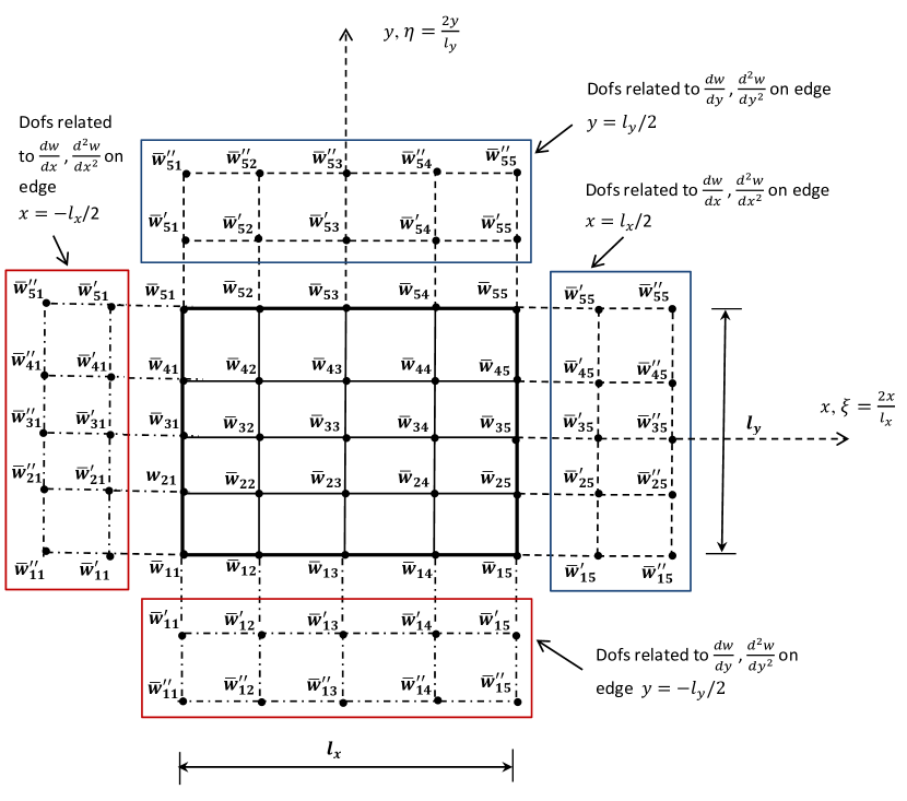
Figure 2: A typical quadrature element for a gradient elastic Kirchhoff plate with $N=N_{x}=N_{y}=5$.

Here, $N=N_{x}=N_{y}=5$ are the number of grid points in $\xi$ and $\eta$ directions, respectively. It can be seen from the Figure 2, the plate element has three degrees of freedom on each edge, five degrees of freedom at the corners and only displacement in the domain. The slope $\bar{w}^{{}^{\prime}}$ and curvature $\bar{w}^{{}^{\prime\prime}}$ dofs related to each edge of the plate are highlighted by the boxes. The transformation used for the plate is $\xi=2x/l_{x}$ and $\eta=2y/l_{y}$ with $-1\leq(\xi,\eta)\leq 1$.

3.1 Lagrange interpolation based quadrature element for gradient elastic plates

The displacement for a $N_{x}\times N_{y}$ node quadrature plate element is assumed as

$$\bar{w}(x,y,t)=\sum_{i=1}^{N}\sum_{j=1}^{N}L_{i}(x)L_{j}(y){w}^{p}_{ij}(t)=\sum_{i=1}^{N}\sum_{j=1}^{N}\bar{L}_{i}(\xi)\bar{L}_{j}(\eta){w}^{p}_{ij}(t)$$ (48)

where $\bar{w}^{p}_{ij}(t)$ is the nodal displacement vector for the plate and $\bar{L}_{i}(\xi)$, $\bar{L}_{j}(\eta)$ are the Lagrange interpolation functions in $\xi$ and $\eta$ directions, respectively. The slope and curvature degrees of freedom at the element boundaries are accounted while computing the weighting coefficients of higher order derivatives as discussed in section 2.1. Substituting the above Equation (48) in Equation (20) we get the stiffness matrix for a gradient elastic quadrature plate element as

$$[K]_{cl}=\frac{ab}{4}\sum_{i=1}^{N}\sum_{j=1}^{N}{H}_{i}{H}_{j}\big{[}{F}(\xi_{i},\eta_{j})\big{]}_{cl}^{T}\,[D]_{cl}\,[{F}(\xi_{i},\eta_{j})]_{cl}$$ (49)

$$[K]_{sg}=g^{2}\frac{ab}{4}\sum_{i=1}^{N}\sum_{j=1}^{N}{H}_{i}{H}_{j}[{F}(\xi_{i},\eta_{j})]_{sg}^{T}\,[D]_{sg}\,[{F}(\xi_{i},\eta_{j})]_{sg}$$ (50)

where ($\xi_{i}$ $\eta_{j})$ and $(H_{i},H_{j})$ are abscissas and weights of GLL quadrature rule. $[F(\xi_{i},\eta_{j})]_{cl}$ and $[F(\xi_{i},\eta_{j})]_{sg}$ are the classical and non-classical strain matrices at location $(\xi_{i},\eta_{j})$ for gradient elastic plate. $[D]_{cl}$ and $[D]_{sg}$ are the constitutive matrices corresponding to classical and gradient elastic plate. The classical and non-classical strain matrices are defined as

$$\big{[}{F}(\xi_{i},\eta_{j})\big{]}_{cl}\{\bar{w}^{p}\}=\begin{bmatrix}{\frac{4}{a^{2}}}{{‎‎\sum}}_{k=1}^{N+4}\bar{B}_{ik}^{\xi}\bar{w}^{p}_{kj}\\ \\ {\frac{4}{b^{2}}}{{‎‎\sum}}_{k=1}^{N+4}\bar{B}_{ik}^{\eta}\bar{w}^{p}_{ik}\\ \\ {\frac{8}{ab}}{{‎‎\sum}}_{l=1}^{N+4}{{‎‎\sum}}_{k=1}^{N+4}\bar{A}_{il}^{\xi}\bar{A}_{jk}^{\eta}\bar{w}^{p}_{lk}\end{bmatrix}\,\,\,\,\,\,(i,j=1,2,..,N)$$ (51)

$$\big{[}{F}(\xi_{i},\eta_{j})\big{]}_{sg}\{\bar{w}^{p}\}=\begin{bmatrix}{g^{2}\frac{8}{a^{3}}}{{‎‎\sum}}_{k=1}^{N+4}\bar{C}_{ik}^{\xi}\bar{w}^{p}_{kj}\\ \\ {g^{2}\frac{8}{b^{3}}}{{‎‎\sum}}_{k=1}^{N+4}\bar{C}_{ik}^{\eta}\bar{w}^{p}_{ik}\\ \\ {g^{2}\frac{8}{{a}^{2}b}}{{‎‎\sum}}_{l=1}^{N+4}{{‎‎\sum}}_{k=1}^{N+4}\bar{B}_{il}^{\xi}\bar{A}_{jk}^{\eta}\bar{w}^{p}_{lk}\\ \\ {g^{2}\frac{8}{a{b}^{2}}}{{‎‎\sum}}_{l=1}^{N+4}{{‎‎\sum}}_{k=1}^{N+4}\bar{A}_{il}^{\xi}\bar{B}_{jk}^{\eta}\bar{w}^{p}_{lk}\end{bmatrix}\,\,\,\,\,\,(i,j=1,2,..,N)$$ (52)

The classical and non-classical constitutive matrices are given as

$$\big{[}D]_{cl}=\begin{bmatrix}\,1&\phantom{-}\mu&\phantom{-}0\\ \\ \,\mu&\phantom{-}1&\phantom{-}0\\ \\ \,0&\phantom{-}0&\phantom{-}2(1-\mu)\end{bmatrix}$$ (53)

$$\big{[}D]_{sg}=\begin{bmatrix}\,1&\phantom{-}0&\phantom{-}\mu&\phantom{-}0\\ \\ \,0&\phantom{-}1&\phantom{-}0&\phantom{-}\mu\\ \\ \,0&\phantom{-}\mu&\phantom{-}(3-2\mu)&\phantom{-}0\\ \\ \,0&\phantom{-}\mu&\phantom{-}0&\phantom{-}(3-2\mu)\end{bmatrix}$$ (54)

The diagonal mass matrix is given by

$$M_{kk}=\frac{\rho{h}ab}{4}H_{i}H{j}\,\,\,\,\,\,\,\,(i,j=1,2,...,N)\,\,\,(k=(i-1)\times N+j)$$ (55)

3.2 Mixed interpolation based quadrature element for gradient elastic plates

The quadrature element presented here is based on mixed Lagrange-Hermite interpolation, with Lagrangian interpolation is assumed in $\xi$ direction and Hermite interpolation in $\eta$ direction. The displacement for a $N_{x}\times N_{y}$ node mixed interpolation quadrature plate element is assumed as

$$\bar{w}(x,y,t)=\sum_{i=1}^{N}\sum_{j=1}^{N+4}L_{i}(x)\Gamma_{j}(y){w}^{p}_{ij}(t)=\sum_{i=1}^{N}\sum_{j=1}^{N+4}\bar{L}_{i}(\xi)\bar{\Gamma}_{j}(\eta){w}^{p}_{ij}(t)$$ (56)

where $\bar{w}^{p}_{ij}(t)$ is the nodal displacement vector of the plate and $\bar{L}_{i}(\xi)$ and $\bar{\Gamma}_{j}(\eta)$ are the Lagrange and Hermite interpolation functions in $\xi$ and $\eta$ directions, respectively. The formulations based on mixed interpolation methods have advantage in excluding the mixed derivative dofs at the free corners of the plate[10]. The modified weighting coefficient matrices derived in section 2.1, using Lagrange interpolations and those given in section 2.2, for Hermite interpolations are used in forming the element matrices. Substituting the above Equation (56) in Equation (20), we get the stiffness matrix for gradient elastic quadrature plate element based on mixed interpolation as

$$[K]_{cl}=\frac{ab}{4}\sum_{i=1}^{N}\sum_{j=1}^{N}{H}_{i}{H}_{j}\big{[}{G}(\xi_{i},\eta_{j})\big{]}_{cl}^{T}\,[D]_{cl}\,[{G}(\xi_{i},\eta_{j})]_{cl}$$ (57)

$$[K]_{sg}=g^{2}\frac{ab}{4}\sum_{i=1}^{N}\sum_{j=1}^{N}{H}_{i}{H}_{j}[{G}(\xi_{i},\eta_{j})]_{sg}^{T}\,[D]_{sg}\,[{G}(\xi_{i},\eta_{j})]_{sg}$$ (58)

where ($\xi_{i}$ $\eta_{j})$ and $(H_{i},H_{j})$ are abscissas and weights of GLL quadrature rule. $[D]_{cl}$ and $[D]_{sg}$ are the classical and gradient elastic constitutive matrices for the plate defined in the section 3.1. The classical $[G(\xi_{i},\eta_{j})]_{cl}$ and non-classical $[G(\xi_{i},\eta_{j})]_{sg}$ strain matrices at the location $(\xi_{i},\eta_{j})$ are defined as,.

$$\big{[}{G}(\xi_{i},\eta_{j})\big{]}_{cl}\{\bar{w}^{p}\}=\begin{bmatrix}{\frac{4}{a^{2}}}{{‎‎\sum}}_{k=1}^{N+4}\bar{B}_{ik}^{(\xi)}\bar{w}^{p}_{kj}\\ \\ {\frac{4}{b^{2}}}{{‎‎\sum}}_{k=1}^{N+4}\bar{\Gamma}_{jk}^{2(\eta)}\bar{w}^{p}_{ik}\\ \\ {\frac{8}{ab}}{{‎‎\sum}}_{l=1}^{N+4}{{‎‎\sum}}_{k=1}^{N+4}\bar{A}_{il}^{(\xi)}\bar{\Gamma}_{jk}^{1(\eta)}\bar{w}^{p}_{lk}\end{bmatrix}\,\,\,\,\,\,(i,j=1,2,..,N)$$ (59)

$$\big{[}{F}(\xi_{i},\eta_{j})\big{]}_{sg}\{\bar{w}^{p}\}=\begin{bmatrix}{g^{2}\frac{8}{a^{3}}}{{‎‎\sum}}_{k=1}^{N+4}\bar{C}_{ik}^{(\xi)}\bar{w}^{p}_{kj}\\ \\ {g^{2}\frac{8}{b^{3}}}{{‎‎\sum}}_{k=1}^{N+4}\bar{\Gamma}_{jk}^{3(\eta)}\bar{w}^{p}_{ik}\\ \\ {g^{2}\frac{8}{{a}^{2}b}}{{‎‎\sum}}_{l=1}^{N+4}{{‎‎\sum}}_{k=1}^{N+4}\bar{\Gamma}_{il}^{2(\xi)}\bar{A}_{jk}^{(\eta)}\bar{w}^{p}_{lk}\\ \\ {g^{2}\frac{8}{a{b}^{2}}}{{‎‎\sum}}_{l=1}^{N+4}{{‎‎\sum}}_{k=1}^{N+4}\bar{\Gamma}_{il}^{1(\xi)}\bar{B}_{jk}^{(\eta)}\bar{w}^{p}_{lk}\end{bmatrix}\,\,\,\,\,\,(i,j=1,2,..,N)$$ (60)

The diagonal mass matrix remains the same as Equation (55). Here, $\bar{A}$, $\bar{B}$ and $\bar{C}$ are the first, second and third order derivatives of Lagrange interpolation functions along the $\xi$ direction. Similarly, $\bar{\Gamma}^{1}$, $\bar{\Gamma}^{2}$ and $\bar{\Gamma}^{3}$ are the first, second and third order derivatives of Hermite interpolation functions in the $\eta$ direction .

4 Numerical Results and Discussion

The efficiency of the proposed quadrature beam and plate element is demonstrate through free vibration analysis. Initially, the convergence study is performed for an Euler-Bernoulli gradient beam, followed by frequency comparisons for different boundary conditions and $g$ values. Similar, study is conducted for a Kirchhoff plate and the numerical results are tabulated and compared with available literature. Four different values of length scale parameters, $g=0.00001,0.05,0.1$, and $0.5$ are considered in this study. Single element is used with GLL quadrature points as nodes to generate all the results reported herein. For results comparison the proposed gradient quadrature beam element based on Lagrange interpolation is designated as SgQE-L and the element based on Hermite interpolation as SgQE-H. Similarly, the plate element based on Lagrange interpolation in $\xi$ and $\eta$ directions as SgQE-LL and the element based on mixed interpolation as SgQE-LH. In this study, the rotary inertia related to slope and curvature degrees of freedom is neglected.

4.1 Quadrature beam element for gradient elasticity theory

The numerical data used for the analysis of beams is as follows: Length $L=1$, Young’s modulus $E=3\times 10^{6}$, Poission’s ratio $\nu=0.3$ and density $\rho=1$. All the frequencies reported for beams are nondimensional as $\bar{\omega}=\omega{L^{2}\sqrt{\rho{A}/EI}}$. Where $A$ and $I$ are area and moment of inertia of the beam and $\omega$ is the natural frequency. The analytical solutions for gradient elastic Euler-Bernoulli beam with different boundary conditions are obtained by following the approach given in [44] and the associated frequency equations are presented in Appendix-I. The classical and non-classical boundary conditions used in the free vibration analysis for different end support are:

Simply supported :
classical :  $w=M=0$ ,    non-classical : $w^{{}^{\prime\prime}}=0$    at $x=(-\frac{L}{2},\frac{L}{2})$

Clamped :
classical :  $w=w^{{}^{\prime}}=0$ ,    non-classical : $w^{{}^{\prime\prime}}=0$    at $x=(-\frac{L}{2},\frac{L}{2})$

Free-free :
classical :  $Q=M=0$ ,    non-classical : $\bar{M}=0$    at $x=(-\frac{L}{2},\frac{L}{2})$

Cantilever :
classical : $w=w^{{}^{\prime}}=0$    at  $x=-\frac{L}{2}$,   $Q=M=0$   at    $x=\frac{L}{2}$     
non-classical : $w^{{}^{\prime\prime}}=0$    at $x=-\frac{L}{2}$ ,   $\bar{M}=0$    at   $x=\frac{L}{2}$     

Propped cantilever :
classical : $w=w^{{}^{\prime}}=0$    at $x=-\frac{L}{2}$ ,   $w=M=0$    at   $x=\frac{L}{2}$     
non-classical : $w^{{}^{\prime\prime}}=0$    at $x=-\frac{L}{2}$ ,   $w^{{}^{\prime\prime}}=0$    at   $x=\frac{L}{2}$     

The size of the displacement vector $\Delta_{d}$ defined in Equation (46) remains as $N-2$ for all the boundary conditions of the beam except for free-free and cantilever beam which are $N$ and $N-1$, respectively. However, the size of the $\Delta_{b}$ vector depends upon the number of non-zero slope and curvature dofs at the element boundaries. The non-classical boundary conditions employed for simply supported gradient beam are $w^{{}^{\prime\prime}}=0$ at $x=(-\frac{L}{2},\frac{L}{2})$, the equations related to curvature degrees of freedom are eliminated and the size of $\Delta_{b}$ is 2. For the gradient cantilever beam the non-classical boundary conditions used are $w^{{}^{\prime\prime}}=0$ at $x=-\frac{L}{2}$ and $\bar{M}=0$ at $x=\frac{L}{2}$. The equation related to curvature degrees of freedom at $x=-\frac{L}{2}$ is eliminated and the equation related to higher order moment at $x=\frac{L}{2}$ is retained and the size of $\Delta_{b}=2$. In the case of clamped beam the non-classical boundary conditions read $w^{{}^{\prime\prime}}=0$ at $x=(-\frac{L}{2},\frac{L}{2})$ and the $\Delta_{b}$ is zero. Similarly, the size for the propped cantilever beam will be 3 as $w^{{}^{\prime\prime}}=0$ at $x=(-\frac{L}{2},\frac{L}{2})$. Finally, for a free-free beam the size of $\Delta_{b}$ vector is 4 due to $\bar{M}=0$ at $x=(-\frac{L}{2},\frac{L}{2})$.

4.1.1 Frequency convergence for gradient elastic quadrature beam elements

In this section, the convergence behaviour of frequencies obtained using proposed SgQE-L and SgQE-H elements for simply supported and free-free Euler-Bernoulli beam are compared. Figure 3, shows the comparison of first three frequencies for a simply supported gradient beam and their convergence trends for $g/L=0.1$. The convergence is seen faster for both SgQE-L and SgQE-H elements for all the three frequencies with solution converging to analytical values with 10 nodes. Similar trend is noticed in the the Figure 4, for free-free beam. It is to be noted that, the proposed SgQE-L and SgQE-H elements are efficient in capturing the rigid body modes associated with the generalized degrees of freedom. The frequencies reported for free-free beam are related to elastic modes and the rigid mode frequencies are not reported here, which are zeros. Hence, single SgQE-L or SgQE-H element with fewer number of nodes can produce accurate solutions even for higher frequencies.

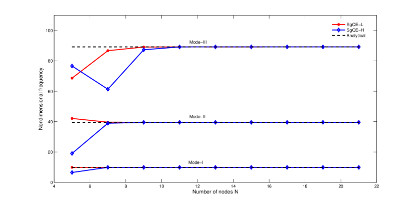
Figure 3: Convergence behaviour of frequencies for a simply supported gradient beam ($g/L=0.1$).

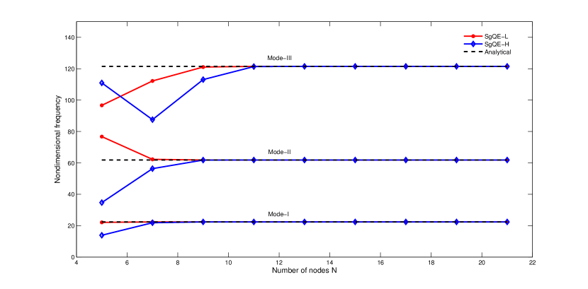
Figure 4: Convergence behaviour of frequencies for a free-free gradient beam ($g/L=0.1$).

4.1.2 Free vibration analysis of gradient beams using SgQE-L and SgQE-H elements

To demonstrate the applicability of the SgQE-L and SgQE-H elements for different boundary conditions the frequencies are compared with the analytical solutions in Tables 1-5. The comparison is made for first six frequencies obtained for different values of $g/L=0.00001,0.05,0.1,0.5$.

Table 1: Comparison of first six frequencies for a simply supported gradient beam

Freq.	$g/L$	0.00001	0.05	0.1	0.5
	SgQE-L	9.869	9.870	9.874	9.984
$\bar{\omega}_{1}$	SgQE-H	9.869	9.871	9.874	9.991
	Analytical	9.870	9.871	9.874	9.991
	SgQE-L	39.478	39.498	39.554	41.302
$\bar{\omega}_{2}$	SgQE-H	39.478	39.498	39.556	41.381
	Analytical	39.478	39.498	39.556	41.381
	SgQE-L	88.826	88.923	89.207	97.725
$\bar{\omega}_{3}$	SgQE-H	88.826	88.925	89.220	98.195
	Analytical	88.826	88.925	89.220	98.195
	SgQE-L	157.914	158.221	159.125	185.378
$\bar{\omega}_{4}$	SgQE-H	157.915	158.225	159.156	186.497
	Analytical	157.914	158.226	159.156	186.497
	SgQE-L	246.740	247.480	249.655	310.491
$\bar{\omega}_{5}$	SgQE-H	247.305	247.475	249.760	313.741
	Analytical	246.740	247.500	249.765	313.743
	SgQE-L	355.344	357.039	361.805	486.229
$\bar{\omega}_{6}$	SgQE-H	355.306	356.766	361.564	488.302
	Analytical	355.306	356.880	361.563	488.240

Table 2: Comparison of first six frequencies for a free-free gradient beam

Freq.	$g/L$	0.00001	0.05	0.1	0.5
	SgQE-L	22.373	22.376	22.387	22.691
$\bar{\omega}_{1}$	SgQE-H	22.373	22.377	22.387	22.692
	Analytical	22.373	22.377	22.387	22.692
$\bar{\omega}_{2}$	SgQE-L	61.673	61.708	61.814	64.841
	SgQE-H	61.673	61.708	61.814	64.856
	Analytical	61.673	61.708	61.814	64.856
	SgQE-L	120.903	121.052	121.496	133.627
$\bar{\omega}_{3}$	SgQE-H	120.904	121.052	121.497	133.710
	Analytical	120.903	121.052	121.497	133.710
	SgQE-L	199.859	202.864	201.553	234.596
$\bar{\omega}_{4}$	SgQE-H	199.876	200.287	201.556	234.875
	Analytical	199.859	200.286	201.557	234.875
	SgQE-L	298.550	299.528	302.422	374.535
$\bar{\omega}_{5}$	SgQE-H	298.556	299.365	302.403	375.234
	Analytical	298.555	299.537	302.443	375.250
	SgQE-L	417.217	419.418	425.469	562.869
$\bar{\omega}_{6}$	SgQE-H	416.991	418.438	424.747	562.758
	Analytical	416.991	418.942	424.697	562.536

In the Table 1, the comparison of first six frequencies for a simply supported gradient beam are shown. For $g/L=0.00001$, all the frequencies match well with the exact frequencies of classical beam. Good agreement with analytical solutions is noticed for all the frequencies obtained using SgQE-L and SgQE-H elements for higher values of $g/L$. In Table 2, the frequencies corresponding to elastic modes are tabulated and compared for a free-free beam. Similarly, in Tables 3-5, comparison in made for cantilever, clamped and propped cantilever gradient beams, respectively. The frequencies obtained using SgQE-L and SgQE-H elements are in close agreement with the analytical solutions for different $g/L$ values. Hence, based on the above findings it can be stated that the SgQE-I and SgQE-II elements can be applied for free vibration analysis of gradient Euler-Bernoulli beam for any choice of boundary conditions and $g/L$ values.

Table 3: Comparison of first six frequencies for a clamped gradient beam

Freq.	$g/L$	0.00001	0.05	0.1	0.5
	SgQE-L	22.324	22.801	23.141	27.747
$\bar{\omega}_{1}$	SgQE-H	22.590	22.845	23.310	27.976
	Analytical	22.373	22.831	23.310	27.976
	SgQE-L	61.540	62.720	63.984	79.450
$\bar{\omega}_{2}$	SgQE-H	62.276	63.003	64.365	79.970
	Analytical	661.673	62.961	64.365	79.970
	SgQE-L	120.392	122.916	125.542	162.889
$\bar{\omega}_{3}$	SgQE-H	122.094	123.594	126.512	164.927
	Analytical	120.903	123.511	126.512	164.927
	SgQE-L	199.427	203.581	208.627	286.576
$\bar{\omega}_{4}$	SgQE-H	201.843	204.502	209.887	289.661
	Analytical	199.859	204.356	209.887	289.661
	SgQE-L	297.282	304.138	312.503	455.285
$\bar{\omega}_{5}$	SgQE-H	301.541	305.843	314.956	462.238
	Analytical	298.555	305.625	314.956	462.238
	SgQE-L	421.194	427.786	442.299	681.749
$\bar{\omega}_{6}$	SgQE-H	421.092	427.787	442.230	691.292
	Analytical	416.991	427.461	442.230	691.292

Table 4: Comparison of first six frequencies for a cantilever gradient beam

Freq.	$g/L$	0.00001	0.05	0.1	0.5
	SgQE-L	3.532	3.545	3.584	3.857
$\bar{\omega}_{1}$	SgQE-H	3.534	3.552	3.587	3.890
	Analytical	3.532	3.552	3.587	3.890
	SgQE-L	21.957	22.188	22.404	24.592
$\bar{\omega}_{2}$	SgQE-H	22.141	22.267	22.497	24.782
	Analytical	22.141	22.267	22.496	24.782
	SgQE-L	61.473	62.150	62.822	71.207
$\bar{\omega}_{3}$	SgQE-H	61.997	62.375	63.094	71.863
	Analytical	61.997	62.375	63.094	71.863
	SgQE-L	120.465	121.867	123.424	146.652
$\bar{\omega}_{4}$	SgQE-H	121.495	122.313	123.966	148.181
	Analytical	121.495	122.313	123.966	148.181
	SgQE-L	199.141	201.636	204.752	257.272
$\bar{\omega}_{5}$	SgQE-H	200.848	202.377	205.658	260.336
	Analytical	202.377	205.658	260.336	200.847
	SgQE-L	297.489	301.551	307.229	410.222
$\bar{\omega}_{6}$	SgQE-H	300.043	302.667	308.605	415.802
	Analytical	300.043	302.667	308.605	415.802

Table 5: Comparison of first six frequencies for a propped cantilever gradient beam

Freq.	$g/L$	0.00001	0.05	0.1	0.5
	SgQE-L	15.413	15.520	15.720	17.351
$\bar{\omega}_{1}$	SgQE-H	15.492	15.581	15.740	17.324
	Analytical	15.492	15.581	15.740	17.324
	SgQE-L	49.869	50.313	51.026	57.767
$\bar{\omega}_{2}$	SgQE-H	50.207	50.512	51.089	58.197
	Analytical	50.207	50.512	51.089	58.197
	SgQE-L	104.044	105.043	106.557	127.127
$\bar{\omega}_{3}$	SgQE-H	104.758	105.457	106.865	128.005
	Analytical	104.758	105.457	106.865	128.005
	SgQE-L	177.922	179.778	182.822	231.247
$\bar{\omega}_{4}$	SgQE-H	179.149	180.500	183.389	233.357
	Analytical	179.149	180.500	183.389	233.357
	SgQE-L	271.502	274.654	280.210	378.692
$\bar{\omega}_{5}$	SgQE-H	273.383	275.749	281.089	382.058
	Analytical	273.383	275.749	281.089	382.058
	SgQE-L	384.785	389.746	399.154	575.841
$\bar{\omega}_{6}$	SgQE-H	387.463	391.341	400.509	582.607
	Analytical	387.463	391.341	400.509	582.607

4.2 Quadrature plate element for gradient elasticity theory

Three different boundary conditions of the plate, simply supported on all edges (SSSS), free on all edges (FFFF) and combination of simply supported and free (SSFF) are considered. The converge behaviour of SgQE-LL and SgQE-LH plate elements is verified first, later numerical comparisons are made for all the three plate conditions for various $g/l_{x}$ values. All the frequencies reported herein for plate are non-dimensional as $\bar{\omega}=\omega{l^{2}_{x}\sqrt{\rho{h}/D}}$. The numerical data used for the analysis of plates is: length $l_{x}=1$, width $l_{y}=1$, thickness $h=0.01$, Young’s modulus $E=3\times 10^{6}$, Poission’s ratio $\nu=0.3$ and density $\rho=1$. The number of nodes in either direction are assumed to be equal, $N=N_{x}=N_{y}$. The choice of the essential and natural boundary conditions for the above three plate problems are given in section 1.2.

The size of the displacement vector $\Delta_{d}$ defined in Equation (46) remains as $(N-2)\times(N-2)$ for all the boundary conditions of the gradient plate except for free-free and cantilever plate which are $N\times N$ and $(N\times N)-N$, respectively. However, the size of the $\Delta_{b}$ vector depends upon the number of non-zero slope and curvature dofs along the element boundaries. The non-classical boundary conditions employed for SSSS gradient plate are $\bar{w}_{xx}=0$ at $x=(-\frac{l_{x}}{2},\frac{l_{x}}{2})$ and $\bar{w}_{yy}=0$ at $y=(-\frac{l_{y}}{2},\frac{l_{y}}{2})$, the equations related to curvature degrees of freedom are eliminated and the size of $\Delta_{b}$ will be $4N-8$, as the $\bar{w}_{x}=\bar{w}_{y}=0$ at the corners of the plate. For a FFFF plate the non-classical boundary conditions employed are $\bar{M}_{x}=0$ at $x=(-\frac{l_{x}}{2},\frac{l_{x}}{2})$ and $\bar{M}_{y}=0$ at $y=(-\frac{l_{y}}{2},\frac{l_{y}}{2})$, and the size of $\Delta_{b}$ is $8N$. Finally, for SSFF plate $\Delta_{b}=6N-4$.

4.2.1 Frequency convergence of gradient elastic quadrature plate elements

In Figure 5, convergence of first three frequencies for a SSSS plate obtained using SgQE-LL and SgQE-LH elements for $g/l_{x}=0.05$ is plotted and compared with analytical solutions[38]. Both SgQE-LL and SgQE-LH elements show excellent convergence behaviour for all the three frequencies. Figures 6 and 7, illustrate the frequency convergence for FFFF and SSFF plates, respectively, for $g/l_{x}=0.05$. Only the SgQE-LL and SgQE-LH element frequencies are shown, as the gradient solution are not available in literature for comparison. It is observed that SgQE-LL and SgQE-LH elements exhibit identical convergence characteristics.

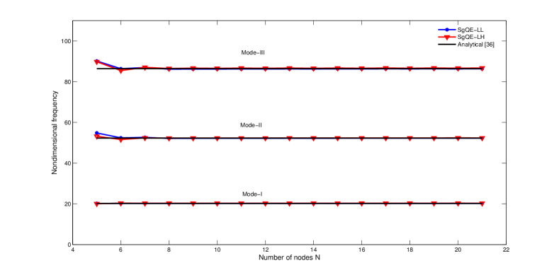
Figure 5: Convergence behaviour of frequencies for a SSSS gradient plate ($g/l_{X}=0.05$).

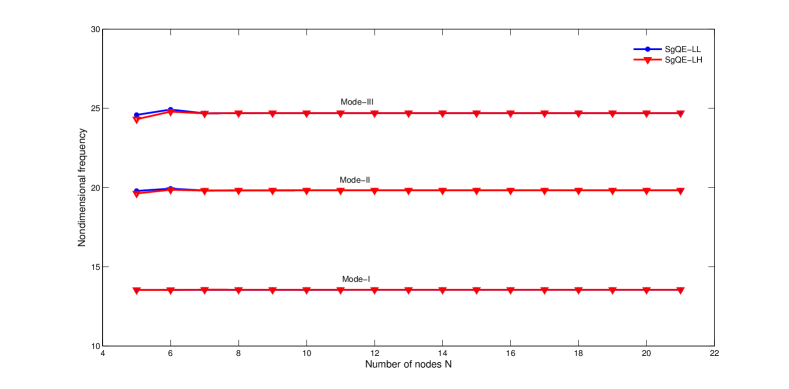
Figure 6: Convergence behaviour of frequencies for a FFFF gradient plate ($g/l_{X}=0.05$).

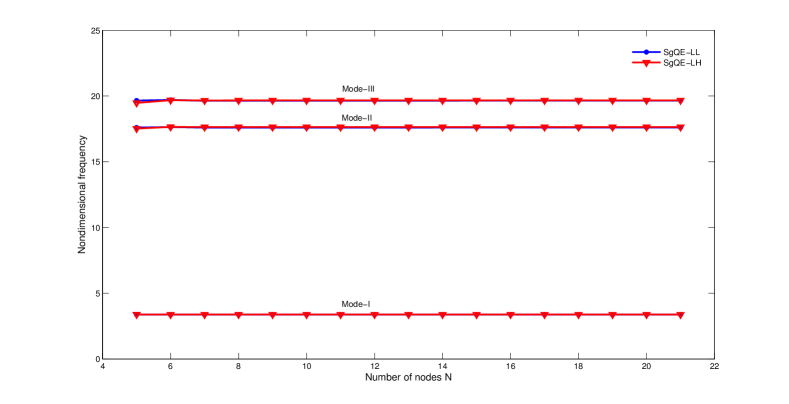
Figure 7: Convergence behaviour of frequencies for a SSFF gradient plate ($g/l_{X}=0.05$).

4.2.2 Free vibration analysis of gradient plate using SgQE-LL and SgQE-LH elements

The first six frequencies for SSSS, FFFF and SSFF plates obtained using SgQE-LL and SgQE-LH elements are compared and tabulated. The comparison is made for different length scale parameter: $g/l_{x}=0.00001,0.05,0.1,0.5$. All the tabulated reslts are generated using $N_{x}=N_{y}=11$ nodes. In the Table 6, the comparison of first six frequencies for SSSS gradient plate are shown. Good agreement with analytical solutions[38] is noticed for all the frequencies obtained using SgQE-LL and SgQE-LH elements for different $g/l_{x}$.

Tables 7 and 8 contains the frequency comparison for FFFF and SSFF plates for various $g/l_{x}$ values. As the exact solutions for gradient elastic plate are not available in the literature for FFFF and SSFF support conditions, the frequencies obtained using SgQE-LL and SgQE-LH are compared. Both elements show identical performance for all $g/l_{x}$ values. The frequencies obtained for lower values of $g/l_{x}=0.00001$ match well with the classical plate frequencies for all support conditions.
In the above findings, SgQE-LL and SgQE-LH elements demonstrate excellent agreement with analytical results for all frequencies and $g/l_{x}$ values for a SSSS plate. For FFFF and SSFF plates, SgQE-LL and SgQE-LH elements produce similar frequencies for $g/l_{x}$ values considered. Hence, a single SgQE-LL or SgQE-LH element with few nodes can be used efficiently to study the free vibration behaviour of gradient plates with different support conditions and $g/l_{x}$ values.

Table 6: Comparison of first six frequencies for a gradient SSSS plate

Freq.	$g/l_{x}$	0.00001	0.05	0.1	0.5
	SgQE-LL	19.739	20.212	21.567	47.693
$\bar{\omega}_{1}$	SgQE-LH	19.739	20.286	21.791	49.940
	Analyt.[38] (m=1,n=1)	19.739	20.220	21.600	48.087
	SgQE-LL	49.348	52.249	60.101	178.418
$\bar{\omega}_{2}$	SgQE-LH	49.348	52.365	60.429	180.895
	Analyt.[38] (m=1,n=2)	49.348	52.303	60.307	180.218
	SgQE-LL	78.957	86.311	105.316	357.227
$\bar{\omega}_{3}$	SgQE-LH	78.957	86.720	106.321	363.156
	Analyt.[38] (m=2,n=2)	78.957	86.399	105.624	359.572
	SgQE-LL	98.696	109.863	137.940	491.447
$\bar{\omega}_{4}$	SgQE-LH	98.696	109.950	138.193	493.131
	Analyt.[38] (m=1,n=3)	98.696	110.201	139.121	500.088
	SgQE-LL	128.305	147.119	192.759	730.346
$\bar{\omega}_{5}$	SgQE-LH	128.305	147.639	193.950	736.599
	Analyt.[38] (m=2,n=3)	128.305	147.454	193.865	737.906
	SgQE-LL	167.783	199.133	272.173	1084.136
$\bar{\omega}_{6}$	SgQE-LH	167.783	199.262	272.486	1085.930
	Analyt.[38] (m=1,n=4)	167.783	199.897	274.562	1099.535

Table 7: Comparison of first six frequencies for a gradient FFFF plate

Freq.	$g/l_{x}$	0.00001	0.05	0.1	0.5
	SgQE-LL	13.468	13.546	13.681	14.118
$\bar{\omega}_{1}$	SgQE-LH	13.468	13.551	13.713	15.628
	Classical[10] (${g/l_{x}}$=0)	13.468	——	——	——
	SgQE-LL	19.596	19.820	20.313	22.113
$\bar{\omega}_{2}$	SgQE-LH	19.596	19.820	20.315	22.129
	Classical[10] (${g/l_{x}}$=0)	19.596	——	——	——
	SgQE-LL	24.270	24.699	25.681	29.745
$\bar{\omega}_{3}$	SgQE-LH	24.270	24.700	25.686	29.785
	Classical[10] (${g/l_{x}}$=0)	24.270	——	——	——
	SgQE-LL	34.8001	35.780	37.929	73.986
$\omega_{4}$	SgQE-LH	34.8001	35.722	38.015	76.161
	Classical[10] (${g/l_{x}}$=0)	34.8001	——	——	——
	SgQE-LL	61.093	64.314	71.238	145.033
$\bar{\omega}_{5}$	SgQE-LH	61.093	64.317	71.244	145.065
	Classical[10] (${g/l_{x}}$=0)	61.093	——	——	——
	SgQE-LL	63.686	67.059	75.114	193.940
$\bar{\omega}_{6}$	SgQE-LH	63.686	67.123	75.509	200.707
	Classical[10] (${g/l_{x}}$=0)	63.686	——	——	——

Table 8: Comparison of first six frequencies for a gradient SSFF plate

Freq.	$g/l_{x}$	0.00001	0.05	0.1	0.5
	SgQE-LL	3.367	3.373	3.386	3.491
$\bar{\omega}_{1}$	SgQE-LH	3.367	3.382	3.413	3.950
	Classical[48, 47] (${g/l_{x}}$=0)	3.367	——	——	——
	SgQE-LL	17.316	17.598	18.370	32.579
$\bar{\omega}_{2}$	SgQE-LH	17.316	17.634	18.474	33.927
	Classical[48, 47] (${g/l_{x}}$=0)	17.316	——	——	——
	SgQE-LL	19.292	19.645	20.585	35.825
$\bar{\omega}_{3}$	SgQE-LH	19.292	19.664	20.649	36.852
	Classical[48, 47] (${g/l_{x}}$=0)	19.292	——	——	——
	SgQE-LL	38.211	39.671	39.162	105.800
$\bar{\omega}_{4}$	SgQE-LH	38.211	39.775	43.851	109.959
	Classical[48, 47] (${g/l_{x}}$=0)	38.211	——	——	——
	SgQE-LL	51.035	53.714	60.400	153.000
$\bar{\omega}_{5}$	SgQE-LH	51.035	53.739	60.493	153.980
	Classical[48, 47] (${g/l_{x}}$=0)	51.035	——	——	——
	SgQE-LL	53.487	56.431	63.699	158.557
$\bar{\omega}_{6}$	SgQE-LH	53.487	56.537	64.000	161.072
	Classical[48, 47] (${g/l_{x}}$=0)	53.487	——	——	——

5 Conclusion

Two novel versions of weak form quadrature elements for gradient elastic beam theory were proposed. This methodology was extended to construct two new and different quadrature plate elements based on Lagrange-Lagrange and mixed Lagrange-Hermite interpolations. A new way to account for the non-classical boundary conditions associated with the gradient elastic beam and plate theories were introduced and implemented. The capability of the proposed four elements was demonstrated through free vibration analysis. Based on the findings it was concluded that, accurate solutions can be obtained even for higher frequencies and for any choice of length scale parameter using single beam or plate element with fewer number of nodes. The new results reported for gradient plate for different boundary conditions can be a reference for the research in this field.

APPENDIX

5.1 Analytical solutions for free vibration analysis of gradient elastic Euler-Bernoulli beam

To obtain the natural frequencies of the gradient elastic Euler-Bernoulli beam which is governed by Equation (9), we assume a solution of the form

$$w(x,t)=\bar{w}(x){e}^{i\omega{t}}$$

substituting the above solution in the governing equation (9), we get

$$\bar{w}^{iv}-g^{2}\bar{w}^{vi}-\frac{\omega^{2}}{\beta^{2}}\bar{w}=0$$

here, $\beta^{2}=EI/m$, and the above equation has the solution of type

$$\bar{w}(x)=\sum_{j=1}^{6}c_{i}{e}^{k_{i}x}$$

where, $c_{i}$ are the constants of integration which are determined through boundary conditions and the $k_{i}$ are the roots of the characteristic equation

$${k}^{iv}-g^{2}{k}^{vi}-\frac{\omega^{2}}{\beta^{2}}=0$$

After applying the boundary conditions listed in section 1.1 we get,

$$[F(\omega)]\{C\}=\{0\}$$

For non-trivial solution, following condition should be satisfied

$$det[F(\omega)]=0$$

The above frequency equation renders all the natural frequencies for a gradient elastic Euler-Bernoulli beam. The following are the frequency equations for different boundary conditions.

(a) Simply supported beam :

$$[F(\omega)]=\begin{bmatrix}1&1&1&1&1&1\\ {e}^{(k_{1}L)}&e^{(k_{2}L)}&e^{(k_{3}L)}&e^{(k_{4}L)}&e^{(k_{5}L)}&e^{(k_{6}L)}\\ \\ {k_{1}}^{2}&{k_{2}}^{2}&{k_{3}}^{2}&{k_{4}}^{2}&{k_{5}}^{2}&{k_{6}}^{2}\\ \\ k_{1}^{2}{e}^{(k_{1}L)}&k_{2}^{2}{e}^{(k_{2}L)}&k_{3}^{2}{e}^{(k_{3}L)}&k_{4}^{2}{e}^{(k_{4}L)}&k_{5}^{2}{e}^{(k_{5}L)}&k_{6}^{2}{e}^{(k_{6}L)}\\ \\ k_{1}^{4}&k_{2}^{4}&k_{3}^{4}&k_{4}^{4}&k_{5}^{4}&k_{6}^{4}\\ \\ k_{1}^{4}{e}^{(k_{1}L)}&k_{2}^{4}{e}^{(k_{2}L)}&k_{3}^{4}{e}^{(k_{3}L)}&k_{4}^{4}{e}^{(k_{4}L)}&k_{5}^{4}{e}^{(k_{5}L)}&k_{6}^{4}{e}^{(k_{6}L)}\\ \\ \end{bmatrix}$$

(b) Cantilever beam :

$$[F(\omega)]=\begin{bmatrix}1&1&1&1&1&1\\ k_{1}&k_{2}&k_{3}&k_{4}&k_{5}&k_{6}\\ \\ {k_{1}}^{2}&{k_{2}}^{2}&{k_{3}}^{2}&{k_{4}}^{2}&{k_{5}}^{2}&{k_{6}}^{2}\\ \\ t_{1}&t_{2}&t_{3}&t_{4}&t_{5}&t_{6}\\ \\ p_{1}&p_{2}&p_{3}&p_{4}&p_{5}&p_{6}\\ \\ k_{1}^{3}{e}^{(k_{1}L)}&k_{2}^{3}{e}^{(k_{2}L)}&k_{3}^{3}{e}^{(k_{3}L)}&k_{4}^{3}{e}^{(k_{4}L)}&k_{5}^{3}{e}^{(k_{5}L)}&k_{6}^{3}{e}^{(k_{6}L)}\\ \\ \end{bmatrix}$$

(c) clamped beam :

$$[F(\omega)]=\begin{bmatrix}1&1&1&1&1&1\\ k_{1}&k_{2}&k_{3}&k_{4}&k_{5}&k_{6}\\ \\ {k_{1}}^{2}&{k_{2}}^{2}&{k_{3}}^{2}&{k_{4}}^{2}&{k_{5}}^{2}&{k_{6}}^{2}\\ \\ {e}^{(k_{1}L)}&{e}^{(k_{2}L)}&{e}^{(k_{3}L)}&{e}^{(k_{4}L)}&{e}^{(k_{5}L)}&{e}^{(k_{6}L)}\\ \\ k_{1}{e}^{(k_{1}L)}&k_{2}{e}^{(k_{2}L)}&k_{3}{e}^{(k_{3}L)}&k_{4}{e}^{(k_{4}L)}&k_{5}{e}^{(k_{5}L)}&k_{6}{e}^{(k_{6}L)}\\ \\ k_{1}^{2}{e}^{(k_{1}L)}&k_{2}^{2}{e}^{(k_{2}L)}&k_{3}^{2}{e}^{(k_{3}L)}&k_{4}^{2}{e}^{(k_{4}L)}&k_{5}^{2}{e}^{(k_{5}L)}&k_{6}^{2}{e}^{(k_{6}L)}\\ \\ \end{bmatrix}$$

(d) Propped cantilever beam :

$$[F(\omega)]=\begin{bmatrix}1&1&1&1&1&1\\ k_{1}&k_{2}&k_{3}&k_{4}&k_{5}&k_{6}\\ \\ {k_{1}}^{2}&{k_{2}}^{2}&{k_{3}}^{2}&{k_{4}}^{2}&{k_{5}}^{2}&{k_{6}}^{2}\\ \\ {e}^{(k_{1}L)}&{e}^{(k_{2}L)}&{e}^{(k_{3}L)}&{e}^{(k_{4}L)}&{e}^{(k_{5}L)}&{e}^{(k_{6}L)}\\ \\ k_{1}^{2}{e}^{(k_{1}L)}&k_{2}^{2}{e}^{(k_{2}L)}&k_{3}^{2}{e}^{(k_{3}L)}&k_{4}^{2}{e}^{(k_{4}L)}&k_{5}^{2}{e}^{(k_{5}L)}&k_{6}^{2}{e}^{(k_{6}L)}\\ \\ p_{1}&p_{2}&p_{3}&p_{4}&p_{5}&p_{6}\\ \\ \end{bmatrix}$$

(e) Free-free beam :

$$[F(\omega)]=\begin{bmatrix}q_{1}&q_{2}&q_{3}&q_{4}&q_{5}&q_{6}\\ \\ r_{1}&r_{2}&r_{3}&r_{4}&r_{5}&r_{6}\\ \\ k_{1}^{3}&k_{2}^{3}&k_{3}^{3}&k_{4}^{3}&k_{5}^{3}&k_{6}^{3}\\ \\ t_{1}&t_{2}&t_{3}&t_{4}&t_{5}&t_{6}\\ \\ p_{1}&p_{2}&p_{3}&p_{4}&p_{5}&p_{6}\\ \\ k_{1}^{3}{e}^{(k_{1}L)}&k_{2}^{3}{e}^{(k_{2}L)}&k_{3}^{3}{e}^{(k_{3}L)}&k_{4}^{3}{e}^{(k_{4}L)}&k_{5}^{3}{e}^{(k_{5}L)}&k_{6}^{3}{e}^{(k_{6}L)}\\ \\ \end{bmatrix}$$

Where,

$t_{1}=(k_{1}^{3}-g^{2}{k_{1}}^{5}){e}^{(k_{1}L)},\quad t_{2}=(k_{2}^{3}-g^{2}{k_{2}}^{5}){e}^{(k_{2}L)},\quad t_{3}=(k_{3}^{3}-g^{2}{k_{3}}^{5}){e}^{(k_{3}L)}$

$t_{4}=(k_{4}^{3}-g^{2}{k_{4}}^{5}){e}^{(k_{4}L)},\quad t_{5}=(k_{5}^{3}-g^{2}{k_{5}}^{5}){e}^{(k_{5}L)}\quad t_{6}=(k_{6}^{3}-g^{2}{k_{6}}^{5}){e}^{(k_{6}L)}$

$p_{1}=(k_{1}^{2}-g^{2}{k_{1}}^{4}){e}^{(k_{1}L)},\quad p_{2}=(k_{2}^{2}-g^{2}{k_{2}}^{4}){e}^{(k_{2}L)},\quad p_{3}=(k_{3}^{2}-g^{2}{k_{3}}^{4}){e}^{(k_{3}L)}$

$p_{4}=(k_{4}^{2}-g^{2}{k_{4}}^{4}){e}^{(k_{4}L)},\quad p_{5}=(k_{5}^{2}-g^{2}{k_{5}}^{4}){e}^{(k_{5}L)},\quad p_{6}=(k_{6}^{2}-g^{2}{k_{6}}^{4}){e}^{(k_{6}L)}$

$q_{1}=(k_{1}^{3}-g^{2}{k_{1}}^{5}),\quad q_{2}=(k_{2}^{3}-g^{2}{k_{2}}^{5}),\quad q_{3}=(k_{3}^{3}-g^{2}{k_{3}}^{5})$

$q_{4}=(k_{4}^{3}-g^{2}{k_{4}}^{5}),\quad q_{5}=(k_{5}^{3}-g^{2}{k_{5}}^{5})\quad q_{6}=(k_{6}^{3}-g^{2}{k_{6}}^{5})$

$r_{1}=(k_{1}^{2}-g^{2}{k_{1}}^{4}),\quad r_{2}=(k_{2}^{2}-g^{2}{k_{2}}^{4}),\quad r_{3}=(k_{3}^{2}-g^{2}{k_{3}}^{4})$

$r_{4}=(k_{4}^{2}-g^{2}{k_{4}}^{4}),\quad r_{5}=(k_{5}^{2}-g^{2}{k_{5}}^{4}),\quad r_{6}=(k_{6}^{2}-g^{2}{k_{6}}^{4})$

References

- [1] Zienkiewicz.O.C, Taylor. R.L., The finite element method,Vol.1. Basic formulations and linear problems, London: McGraw-Hill, 1989,648p.
- [2] Zienkiewicz.O.C, Taylor. R.L., The finite element method, Vol.2. Solid and fluid mechanics: dynamics and non-linearity, London: McGraw-Hill, 1991, 807p.
- [3] K.J. Bathe., Finite element procedures in engineering analysis. Prentice-Hall, 1982.
- [4] Bellman RE, Casti J., Differential quadrature and long-term integration. Journal of Mathematical Analysis and Applications 1971; 34:235–238.
- [5] Bert, C. W., and Malik, M., 1996,“Differential Quadrature Method in Compu-tational Mechanics: A Review,”. ASME Appl. Mech. Rev., 49(1), pp. 1–28.
- [6] Bert, C. W., Malik, M., 1996,“The differential quadrature method for irregular domains and application to plate vibration.”. International Journal of Mechanical Sciences 1996; 38:589–606.
- [7] C. Shu, Differential Quadrature and Its Application in Engineering,. Springer-Verlag, London, 2000.
- [8] H. Du, M.K. Lim, N.R. Lin, Application of generalized differential quadrature method to structural problems,. Int. J. Num. Meth.Engrg. 37 (1994) 1881–1896.
- [9] H. Du, M.K. Lim, N.R. Lin, Application of generalized differential quadrature to vibration analysis,. J. Sound Vib. 181 (1995) 279–293.
- [10] Xinwei Wang, Differential Quadrature and Differential Quadrature Based Element Methods Theory and Applications,.Elsevier, USA, 2015
- [11] O. Civalek, O.M. Ulker., Harmonic differential quadrature (HDQ) for axisymmetric bending analysis of thin isotropic circular plates,. Struct. Eng. Mech.17 (1) (2004) 1–14.
- [12] O. Civalek, Application of differential quadrature (DQ) and harmonic differential quadrature (HDQ) for buckling analysis of thin isotropic plates and elastic columns. Eng. Struct. 26 (2) (2004) 171–186.
- [13] X. Wang, H.Z. Gu, Static analysis of frame structures by the differential quadrature element method,. Int. J. Numer. Methods Eng. 40 (1997) 759–772.
- [14] X. Wang, Y. Wang, Free vibration analysis of multiple-stepped beams by the differential quadrature element method, Appl. Math. Comput. 219 (11) (2013) 5802–5810.
- [15] Wang Y, Wang X, Zhou Y., Static and free vibration analyses of rectangular plates by the new version of differential quadrature element method, International Journal for Numerical Methods in Engineering 2004; 59:1207–1226.
- [16] Y. Xing, B. Liu, High-accuracy differential quadrature finite element method and its application to free vibrations of thin plate with curvilinear domain, Int. J. Numer. Methods Eng. 80 (2009) 1718–1742.
- [17] Malik M., Differential quadrature element method in computational mechanics: new developments and applications. Ph.D. Dissertation, University of Oklahoma, 1994.
- [18] Karami G, Malekzadeh P., A new differential quadrature methodology for beam analysis and the associated differential quadrature element method. Computer Methods in Applied Mechanics and Engineering 2002; 191:3509–3526.
- [19] Karami G, Malekzadeh P., Application of a new differential quadrature methodology for free vibration analysis of plates. Int. J. Numer. Methods Eng. 2003; 56:847–868.
- [20] A.G. Striz, W.L. Chen, C.W. Bert, Static analysis of structures by the quadrature element method (QEM),. Int. J. Solids Struct. 31 (1994) 2807–2818.
- [21] W.L. Chen, A.G. Striz, C.W. Bert, High-accuracy plane stress and plate elements in the quadrature element method, Int. J. Solids Struct. 37 (2000) 627–647.
- [22] H.Z. Zhong, Z.G. Yue, Analysis of thin plates by the weak form quadrature element method, Sci. China Phys. Mech. 55 (5) (2012) 861–871.
- [23] Chunhua Jin, Xinwei Wang, Luyao Ge, Novel weak form quadrature element method with expanded Chebyshev nodes, Applied Mathematics Letters 34 (2014) 51–59.
- [24] T.Y. Wu, G.R. Liu, Application of the generalized differential quadrature rule to sixth-order differential equations, Comm. Numer. Methods Eng. 16 (2000) 777–784.
- [25] G.R. Liu a , T.Y. Wu b, Differential quadrature solutions of eighth-order boundary-value differential equations, Journal of Computational and Applied Mathematics 145 (2002) 223–235.
- [26] Xinwei Wang, Novel differential quadrature element method for vibration analysis of hybrid nonlocal Euler–Bernoulli beams, Applied Mathematics Letters 77 (2018) 94–100.
- [27] Mindlin, R.D., 1965.1964. Micro-structure in linear elasticity. Arch. Rat. Mech. Anal. 16, 52–78.
- [28] Mindlin, R., Eshel, N., 1968. On first strain-gradient theories in linear elasticity. Int. J. Solids Struct. 4, 109–124.
- [29] Mindlin, R.D., 1965.1964. Micro-structure in linear elasticity. Arch. Rat. Mech. Anal. 16, 52–78.
- [30] Fleck, N.A., Hutchinson, J.W., A phenomenological theory for strain gradient effects in plasticity. 1993. J. Mech. Phys. Solids 41 (12), 1825e1857.
- [31] Koiter, W.T., 1964.Couple-stresses in the theory of elasticity, I & II. Proc. K. Ned.Akad. Wet. (B) 67, 17–44.
- [32] Harm Askes, Elias C. Aifantis, Gradient elasticity in statics and dynamics: An overview of formulations,length scale identification procedures, finite element implementations and new results Int. J. Solids Struct. 48 (2011) 1962–1990
- [33] Aifantis, E.C., Update on a class of gradient theories. 2003.Mech. Mater. 35,259e280.
- [34] Altan, B.S., Aifantis, E.C., On some aspects in the special theory of gradient elasticity. 1997. J. Mech. Behav. Mater. 8 (3), 231e282.
- [35] Papargyri-Beskou, S., Tsepoura, K.G., Polyzos, D., Beskos, D.E., Bending and stability analysis of gradient elastic beams. 2003. Int. J. Solids Struct. 40, 385e400.
- [36] S. Papargyri - Beskou, D. Polyzos, D. E. Beskos, Dynamic analysis of gradient elastic flexural beams. Structural Engineering and Mechanics, Vol. 15, No. 6 (2003) 705–716.
- [37] A.K. Lazopoulos, Dynamic response of thin strain gradient elastic beams, International Journal of Mechanical Sciences 58 (2012) 27–33.
- [38] Papargyri-Beskou, S., Beskos, D., Static, stability and dynamic analysis of gradient elastic flexural Kirchhoff plates. 2008. Arch. Appl. Mech. 78, 625e635.
- [39] Lazopoulos, K.A., On the gradient strain elasticity theory of plates. 2004. Eur. J.Mech. A/Solids 23, 843e852.
- [40] Papargyri-Beskou, S., Giannakopoulos, A.E., Beskos, D.E., Variational analysis of gradient elastic flexural plates under static loading. 2010. International Journal of Solids and Structures 47, 2755e2766.
- [41] I. P. Pegios · S. Papargyri-Beskou · D. E. Beskos, Finite element static and stability analysis of gradient elastic beam structures, Acta Mech 226, 745–768 (2015).
- [42] Tsinopoulos, S.V., Polyzos, D., Beskos, D.E, Static and dynamic BEM analysis of strain gradient elastic solids and structures, Comput. Model. Eng. Sci. (CMES) 86, 113–144 (2012).
- [43] Vardoulakis, I., Sulem, J., Bifurcation Analysis in Geomechanics. 1995. Blackie/Chapman and Hall, London.
- [44] Kitahara, M. (1985), Boundary Integral Equation Methods in Eigenvalue Problems of Elastodynamics and Thin Plates, Elsevier, Amsterdam.
- [45] J.N. Reddy, Energy Principles and Variational Methods in Applied Mechanics, Second Edition, John Wiley, NY, 2002.
- [46] S.P. Timoshenko, D.H. Young, Vibration Problem in Engineering, Van Nostrand Co., Inc., Princeton, N.J., 1956.
- [47] B.Singh, S. Chakraverty, Flexural vibration of skew plates using boundary characteristics orthogonal polynomials in two variables, J. Sound Vib. 173 (2) (1994) 157–178.
- [48] A.W. Leissa, The free vibration of rectangular plates, J. Sound Vib. 31 (3) (1973) 257–293.