Graph Operator Modeling over Large Graph Datasets
(Extended Version)

Abstract

As graph representations of data emerge in multiple domains, data analysts need to be able to intelligently select among a magnitude of different data graphs based on the effects different graph operators have on them. Exhaustive execution of an operator over the bulk of available data sources is impractical due to the massive resources it requires. Additionally, the same process would have to be re-implemented whenever a different operator is considered. To address this challenge, this work proposes an efficient graph operator modeling methodology. Our novel approach focuses on the inputs themselves, utilizing graph similarity to infer knowledge about input graphs. The modeled operator is only executed for a small subset of the available graphs and its behavior is approximated for the rest of the graphs using machine learning techniques. Our method is operator-agnostic, as the same similarity information can be reused for modeling multiple graph operators. We also propose a family of similarity measures based on the degree distribution that prove capable of producing high quality estimations, comparable or even surpassing other much more costly, state-of-the-art similarity measures. Our evaluation over both real-world and synthetic graphs indicates that our method achieves extremely accurate modeling of many commonly encountered operators, managing massive speedups over a brute-force alternative.

1 Introduction

Graph Analytics has been gaining an increasing amount of attention in recent years. Driven by the surge in social and business graph data, graph analytics is used to effectively tackle complex tasks in many areas such as bioinformatics, social community analysis, traffic optimization, fraud detection, etc. A diverse collection of graph operators exists [14], with functionality typically including the computation of centrality measures, clustering metrics or network statistics [10].

Yet, as Big Data technologies mature and evolve (with regular advances in Big Graph Systems [39]), emphasis is placed on areas not solely related to data (i.e., graph) size. A different type of challenge steadily shifts attention to the actual content: In content-based analytics [17], data from social media platforms is processed for sense-making. Similarly, in content-sensitive applications such as recommendation systems, web advertising, credit analysis, etc., the quality of the insights derived is mainly attributed to the input content. The plethora of available sources for content-sensitive analytics tasks now creates an issue: Data scientists need to decide which of the available datasets should be fed to a given workflow independently, in order to maximize its impact. Yet, as modern analytics tasks have evolved into increasingly long and complex series of diverse operators, evaluating the utility of immense numbers of inputs is prohibitively expensive. This is notably true for graph operators, whose computational cost has led to extensive research on approximation algorithms (e.g., [34, 15]).

As a motivating example, let us consider a dataset consisting of a very large number of citation graphs. We wish to identify the graphs that have the most well-connected citations and contain highly cited papers. The clustering coefficient [10], a good measure of neighborhood connectivity, would have to be computed for all the graphs in the dataset in order to allow the identification of the top-k such graphs. To quantify the importance of each paper, we consider a centrality measure such as betweenness centrality [10]. Consequently, we would have to compute the maximum betweenness centrality score for each citation graph and combine the results with those obtained from the analysis based on the clustering coefficient. Yet, this is a daunting task due to the operators’ complexity and the number of executions required. It is not straight-forward how the different input graphs affect the output of the clustering coefficient or betweenness centrality metrics. For traditional algorithms, performance is driven by algorithmic complexity usually tied to the input size. In Big Data Analytics, such analyses cannot be intuitively deduced [22].

The challenge this work tackles is thus the following: Given a graph analytics operator and a large number of input graphs, can we reliably predict operator output for every input graph at low cost? How can we rank or tangibly characterize input datasets relative to their effect on job execution? In this work, we introduce a novel, operator-agnostic dataset profiling mechanism: Rather that executing the operator over each input separately, our work assesses the relationship between the dataset’s graphs. Based on graph similarity, we infer knowledge about them. In our example, instead of exhaustively computing the clustering coefficient, we calculate a similarity matrix for our dataset, compute the clustering coefficient for a small subset of graphs and utilize the similarity matrix to estimate its remaining values. We may then compute the maximum betweenness centrality for also a small subset of citation graphs and reuse the already calculated similarity matrix to estimate betweenness centrality scores for the rest of the graphs.

Our method is based on the intuition that, for a given graph operator, similar graphs produce similar outputs. This intuition is solidly supported by the existence of strong correlations between different graph operators ([26, 9, 24]). Hence, by assuming a similarity measure that correlates to a set of operators, we can use machine learning techniques to approximate their outcomes. Given a graph dataset and an operator to model, our method utilizes a similarity measure to compute the similarity matrix of the dataset, i.e., all-pairs similarity scores between the graphs of the dataset. The given operator is then run for a small subset of the dataset; using the similarity matrix and the available operator outputs, we are able to approximate the operator for the remaining graphs. To the best of our knowledge, this is the first effort to predict graph operator output over very large numbers of available inputs. In summary, we make the following contributions in this work:

• We propose a novel, similarity-based method to estimate graph operator output for very large numbers of input graphs. The method shifts the complexity of numerous graph computations to less expensive pairs of similarities. This choice offers two major advantages: First, our scheme is operator-agnostic: The resulting similarity matrix can be reused by different operators, amortizing its computation cost. As a result, the cost of our method is ultimately dominated by the computation of that operator for a small subset of the dataset. Second, the method is agnostic to the similarity measure that is used. This property gives us the ability to utilize or arbitrarily combine different similarity measures.

• We introduce a family of similarity measures based on the degree distribution with a gradual tradeoff between detail and computation complexity. Despite their simplicity, they prove capable of producing high quality estimations, comparable or even surpassing other more costly, state-of-the-art similarity measures ([36, 38]).

• We improve on the complexity of the similarity matrix computation by providing an alternative to calculating all-pairs similarity scores. We propose, instead, to initially cluster a given dataset to groups of similar graphs using the inverse of the similarity measure as a distance metric. Then, calculate all-pairs similarities for each cluster, assuming inter-cluster similarity scores to equal zero. In our experimental evaluation we observe that this approach can lead to up to $15\times$ speedup in similarity matrix calculations while having little to no effect on modeling accuracy.

• We offer an open-source implementation of our method and perform an extensive experimental evaluation using both synthetic and real datasets. Our results indicate that the similarity-based approach is accurately modeling a variety of popular graph operators, with errors even $<1\%$, sampling a mere $5\%$ of the graphs for execution. Amortizing the similarity cost over six operators, modeling is sped up to $18\times$ compared to exhaustive modeling. Our proposed similarity measures produce similar or more accurate results compared to state-of-the-art similarity measures but run more than $5$ orders of magnitude faster. Finally, our analysis provides insights on the connection between different operators and the respective similarity functions, demonstrating the utility of similarity matrix composition.

2 Methodology

In this section, we formulate the problem and describe the methodology along with different aspects of the proposed solution. We start off with some basic notation followed throughout the paper and a formal description of our method and its complexity.

Let a graph $G$ be an ordered pair $G=(V,E)$ with $V$ being the set of vertices and $E$ the set of edges of $G$, respectively. The degree of a vertex $u\in V$, denoted by $d_{G}(u)$, is the number of edges of $G$ incident to $u$. The degree distribution of a graph $G$, denoted by $P_{G}(k)$, expresses the probability that a randomly selected vertex of $G$ has degree $k$. A dataset $D$ is a set of $N$ simple, undirected graphs $D=\{G_{1},G_{2},...,G_{N}\}$. We define a graph operator to be a function $g\colon D\to\mathbb{R}$, mapping an element of $D$ to a real number. In order to quantify the similarity between two graphs $G_{a},G_{b}\in D$ we use a graph similarity function $s\colon D\times D\to\mathbb{R}$ with range within $[0,1]$. For two graphs $G_{a},G_{b}\in D$, a similarity of $1$ implies that they are identical while a similarity of $0$ the opposite.

Consequently, the problem we are addressing can be formally stated as follows: Given a dataset of graphs $D$ and a graph operator $g$, without knowledge of the range of $g$ given $D$, we wish to infer a function $\hat{g}\colon D\to\mathbb{R}$ that approximates $g$. Additionally, we wish our approximation to be both accurate (i.e., $|g-\hat{g}|<\epsilon$, for some small $\epsilon$) and efficient (i.e., $O(\hat{g})<O(g)$). We observe that, although this formulation resembles a function approximation problem, the two additional requirements mentioned differentiate it from a typical problem of this class. In such problems, we have knowledge of the entire output space of $g$ for a given dataset. Moreover, no complexity restrictions are posed. In this formulation, our goal is to provide an accurate approximation of $g$, while avoiding its exhaustive execution over the entire $D$.

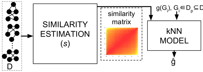
Figure 1: Methodology Pipeline

To achieve this goal, we utilize the similarity matrix $R$, an $N\times N$ matrix with $R[i,j]=s(G_{i},G_{j})$, where $s$ is a given similarity measure. As a result, $R$ contains all-pairs similarity scores between the graphs of $D$. $R$ is symmetric, its elements are in $[0,1]$ and the entries of its main diagonal equal $1$. Our method takes as input a dataset $D$ and an operator $g$ to model. It forms the pipeline depicted in Figure 1: It begins with the computation of the similarity matrix $R$ based on $s$; it calculates the actual values of $g$ for a ratio $p\in(0,1)$ of randomly selected graphs of $D$, referred to as $D_{p}$. Finally, it estimates $g$ for the remaining graphs of $D$ by running a weighted version of the $k$-Nearest-Neighbors (kNN) algorithm [23]. The inferred function $\hat{g}$ is then given by the following equation:

$$\hat{g}(G_{x})=\frac{\sum_{i\in\Gamma_{k}(x)}w_{xi}g(G_{i})}{\sum_{i\in\Gamma_{k}(x)}w_{xi}}$$ (1)

Where $w_{xi}=R[x,i]$ is the similarity score for graphs $G_{x},G_{i}$, i.e., $w_{xi}=s(G_{x},G_{i})$, $\Gamma_{k}(x)$ is the set of the $k$ most similar graphs to $G_{x}$ for which we have already calculated $g$ and $g(G_{i})$ the value of the operator for $G_{i}$. Our approach is formally described in Algorithm 1.

Algorithm 1 Graph Operators Modeling

1:procedure Approximate($[G_{1},...,G_{N}]$, $g$, $s$, $p$, $k$)

2:     $R\leftarrow[\ ],T\leftarrow\{\ \},A\leftarrow\{\ \}$

3:     for $(i,j)\leftarrow[1,N]\times[1,N]$ do

4:         $R[i,j]\leftarrow s(G_{i},G_{j})$      

5:     for $i\leftarrow 1,p\cdot N$ do

6:         $r\leftarrow randint(1,N)$

7:         $T[G_{r}]\leftarrow g(G_{r})$      

8:     for $x\leftarrow[G_{1},G_{2},...,G_{N}],x\notin keys(T)$ do

9:         $t\leftarrow findNeighbors(R,T,k,x)$

10:         $A[x]\leftarrow calcApproximation(R,t)$      

11:     return $A$

The complexity of Algorithm 1 can be broken down to its three main components. First, there is the calculation of the similarity matrix $R$ in lines $3-4$, which, for a given similarity measure $s$ with complexity $S$, runs in $O(N^{2}S)$. The second component (lines $5-7$), which computes the operator $g$ for $pN$ graphs, has complexity $O(pNM)$, assuming that $g$ has complexity of $M$. The approximation of the operator for the remaining graphs (lines $8-10$) runs in $O((N(1-p))((pN)log(pN)+k))$ since, for each of the remaining dataset graphs (which are $N(1-p)$), we first sort the similarities of our training set ($T$) in order to find the $k$ nearest neighbors to each unknown point ($findNeighbors$), an operation of $O((pN)log(pN))$ complexity. We then perform $k$ iterations to calculate the weighted sum of Equ. 1 ($calcApproximation$). Thus, the complexity of our method is:

$$O(N^{2}S+pNM+(N(1-p))((pN)log(pN)+k))$$ (2)

From Equ. 2, we deduce that the complexity of our method is dominated by its first two components. Consequently, the lower the computational cost of $s$, the more practical our approach will be. Additionally, we expect our training set to be much smaller than our original dataset (i.e., $p\ll 1$), otherwise the second component will approach $NM$, which is no different that calculating the operator for the entire dataset.

It is important to note here that the $O(N^{2}S)$ component corresponds to a calculation performed only once, whether modeling a single or multiple operators. Indeed, as we show in this work, there exist both intuitive and simple to compute operators that can be utilized for a number of different graph tasks. Moreover, our methodology allows for composition of similarity matrices, permitting combinations of different measures. Given that the similarity matrix calculation happens once per dataset, its cost gets amortized over multiple graph operators, making the $O(pNM)$ factor the dominant one for our pipeline.

2.1 Similarity Measures

The similarity matrix is an essential tool in our efforts to model graph operators under the hypothesis that similar graphs produce similar operator outputs. This would also suggest a connection between the similarity measure and the graph operators we consider. Relative to graph analytics operators, we propose a family of similarity measures based on graph degree distribution. Reinforced by the proven correlations between many diverse graph operators ([26, 9, 24]), we intend the proposed similarity measures to express graph similarity in a way that enables modeling of multiple operators at low cost.

$\triangleright$ Degree Distribution: In order to quantify the similarity between two graphs we rely on comparing their degree distributions. We compute the degree distributions from the graph edge lists and compare them using the Bhattacharyya coefficient BC [6]. BC is considered a highly advantageous method for comparing distributions [1].

BC divides the output space of a function into $m$ partitions and uses the cardinality of each partition to create an $m$-dimensional vector representing that space. As a measure of divergence between two distributions, the square of the angle between the two vectors is considered. BC is thus calculated by: $BC(q,r)=\sum_{i=1}^{m}\sqrt{q_{i}r_{i}}$, where $q$, $r$ are the two samples, $m$ the number of partitions created by the algorithm and $q_{i}$, $r_{i}$ the cardinality of the $i$-th partition of each sample. In our case, the two samples represent the graphs we intend to compare and the points in our space are the degrees of the nodes of each graph. By dividing that space into partitions and considering the cardinalities of each partition, we effectively compare the degree distributions of those graphs.

In our implementation, we use a $k$-d tree [5], a data structure used for space partitioning to compute BC. We build a $k$-d tree once, based on a predefined percentage of vertex degrees from all the graphs in $D$. We then use the created space partitioning to compute degree distributions for each graph. By using the median of medians algorithm [12], this process has complexity $O(\nu log\nu+N|V|log\nu)$, where $\nu$ is the number of vertices used to build the tree.

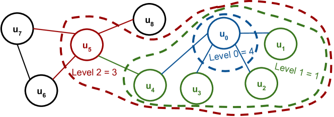
Figure 2: Example of Degree Distribution + Levels

$\triangleright$ Degree Distribution + Levels: As an extension of the degree distribution-based similarity measure, we consider a class of measures with increasing levels of information. The intuition behind it is that the degree of a vertex is a measure of its connectivity based on its immediate neighbors. For instance, we can define the degree of a vertex at level 1 as the degree of a supernode containing the vertex and all its immediate neighbors. Internal edges of the supernode do not contribute to his degree. Generalizing this idea to more than one levels gives us a measure of the indirect connectivity of a vertex. By combining the degrees of a vertex for multiple levels we get information about its connectivity up to level hops away. As an illustrative example, in Figure 2 vertex $u_{0}$ has degree 4, when considering its direct neighbors. When its neighborhood is expanded to level 1, $u_{0}$’s degree is 1 and for level 2 it becomes 3.

Based on this idea, we quantify the similarity between graphs by calculating the degrees up to a certain level for each vertex of the graphs and use BC to compare the resulting degree distributions. A good property of this class of measures is that they provide us with a nice tradeoff between accuracy and computational cost. Increasing the number of degree distribution levels involves additional computations but also incorporates more graph topological insights to it. In order to calculate the degrees for a given level, for each vertex we perform a depth-limited Depth First Search up to level hops away in order to mark the internal edges of the supernode. We then count the edges of the border vertices (vertices level hops away from the source) that do not connect to any internal vertices. The complexity of this algorithm is $\mathcal{O}(|V|(\overline{d})^{l})$ where $\overline{d}$ is the average branching factor (average degree) and $l$ the level-depth limit.

$\triangleright$ Degree Distribution + Vertex Count A second extension to our degree distribution-based similarity measure is based on the ability of our method to combine similarity matrices. Graph size, in terms of vertex count, is another graph attribute to measure similarity on. We formulate similarity in terms of vertex count as: $s(G_{i},G_{j})=\frac{min(|V_{G_{i}}|,|V_{G_{j}}|)}{max(|V_{G_{i}}|,|V_{G_{j}}|)}$. Intuitively, $s$ approaches $1$ when $|V_{G_{i}}|-|V_{G_{j}}|$ approaches $0$, i.e., when $G_{i},G_{j}$ have similar vertex counts. To incorporate vertex count into the graph comparison, we can combine the similarity matrices computed with degree distributions and vertex counts using an arbitrary formula (e.g., linear composition).

2.2 Similarity Matrix Computation Speedup

Based on Equ. 2, the complexity of our method is primarily dominated by the first two components and specifically by the similarity matrix calculation. Although it refers to a one time computation and its cost is being amortized with modeling of multiple graph operators, having to compute all-pairs similarity scores for a large collection of graphs can be prohibitively expensive (in the order of $O(N^{2})$ for $N$ graphs). Here, we introduce a preprocessing step which we argue that improves the existing computational cost, reducing the number of similarity calculations performed.

As, in order to approximate a graph operator, we employ kNN, we observe that, for each graph, we only require the similarity scores to its $k$ most similar graphs for which we have the value of $g$, i.e., the weights in Equ. 1. The remaining similarity scores involving this graph are not used. Therefore we propose, as a first step, to run a clustering algorithm which will produce clusters of graphs with high similarity. Then for each cluster compute all-pairs similarity scores between its members. Inter-cluster similarities are assumed to be zero and are not computed. By creating clusters of size much larger than $k$, we expect minimal loss in accuracy while avoiding a considerable number of similarity computations.

As a clustering algorithm we use a simplified version of $k$-medoids in combination with $k$-means++, for the initial seed selection ([28, 2]). We aim at creating clusters much larger than the required $k$ elements of kNN and therefore do not consider necessary to recalculate the cluster medoids at each iteration of the $k$-medoids algorithm. In addition, we rely on $k$-means++ to spread out the cluster medoids, something that has been proven to give better clustering results [2]. Consequently, our approach runs $k$-means++ to find $k$ cluster centers and groups the graphs based on their distances to those centers. Then, for each cluster computes all-pairs similarity scores between its members. As a distance measure we consider the inverse of the similarity measure we employ, that is $d(G_{i},G_{j})=1-s(G_{i},G_{j})$. Assuming the produced cluster sizes are close to $\frac{N}{c}$, $c$ being the number of clusters created, the similarity computations performed are in the order of $O(\frac{N^{2}}{c}+Nc)$ . Thus, by setting $c=\sqrt{N}$ we can achieve $O(N\sqrt{N})$ similarity computations for a dataset of $N$ graphs.

2.3 Discussion

In this section, we consider a series of issues that relate to the configuration and performance of our method as well as to the relation between modeled operators, similarity measure and input datasets.

$\triangleright$ Graph Operators: In this work, we focus on graph analytics operators, namely centralities, clustering metrics, network statistics, etc. Research on this area has resulted in a large collection of operators, also referred to as topology metrics, with new ones being constantly added (e.g., [14, 10, 9, 24]). Topology metrics can be loosely classified in three broad categories ([26, 9, 24]): Those related to distance, connectivity and spectrum. In the first class, we find metrics that involve distances between vertices such as diameter, average distance and betweenness centrality. The second class relates to vertex degrees containing metrics such as average degree, degree distribution, clustering coefficient, etc. Finally, the third class comes from the spectral analysis of a graph and contains the computation of eigenvalues, the corresponding eigenvectors or other spectral-related metrics.
$\triangleright$ Similarity Matrix and Graph Operators: An aspect we take under consideration is the similarity measure we employ in relation to the graph operator we intend to model. Research has identified strong correlations between certain classes of graph operators, for example topology metrics ([26, 9, 24]). It is thus safe to assume that if, for example, we base our similarity calculations on a degree-related measure, we should be more successful in modeling degree-related graph operators than distance-related. In practice, the analyst should have some level of intuition on the type of graph operators to be modeled. In our experimental evaluation, we model operators from all three aforementioned operator classes in order to evaluate the efficiency of the proposed similarity measures.
$\triangleright$ Combining Similarity Measures: We can think of use cases where we want to quantify the similarity of graphs based on parameters unrelated to each other which cannot be expressed by a single similarity measure. For example, we might want to compare two graphs based on their degree distributions but also take under account their order (vertex count). Essentially, we would like to be able to combine multiple independent similarity measures. This composition can be naturally implemented in our system. We can compute independent similarity matrices for each of our similarity measures and “fuse” those matrices into one based on a given formula. This technique is presented in our experimental evaluation and proves effective in a number of operators.
$\triangleright$ Regression Analysis Although there exist several approaches to statistical learning [23], we have opted for the kNN method. We choose kNN for its simplicity and because we do not have to calculate distances between points of our dataset (we already have that information from the similarity matrix). The kNN algorithm is also suitable for our use case since it is sensitive to localized data and insensitive to outliers. A desired property, since we expect similar graphs to have similar operator scores and should therefore be of influence in our estimations. Conversely, we expect operator scores for graphs of low similarity to have little or no influence on score estimations.

3 Experimental Evaluation

3.1 Experimental Setup

$\triangleright$ Datasets: For our experimental evaluation, we consider both real and synthetic datasets. The real datasets comprise a set of ego graphs from Twitter (TW) which consists of 973 user “circles” as well as a dataset containing 733 snapshots of the graph that is formed by considering the Autonomous Systems (AS) that comprise the Internet as nodes and adding links between those systems that communicate to each other. Both datasets are taken from the Stanford Large Network Dataset Collection [30].

We also experiment with a dataset of synthetic graphs (referred to as the BA dataset) generated using the SNAP library [31]. We use the GenPrefAttach generator to create random scale-free graphs with power-law degree distributions using the Barabasi-Albert model [4]. The degree distribution of the synthetic graphs, according to this model, can be given by: $P(k)\sim k^{-\gamma}$, where $\gamma=3$. We keep the vertex count of the graphs constant to 4K. We introduce randomness to this dataset by having the initial outdegree of each vertex be a uniformly random number in the range $[1,32]$. The Barabasi-Albert model constructs a graph by adding one vertex at a time. The initial outdegree of a vertex is the maximum number of vertices it connects to, the moment it is added to the graph. The graphs of the dataset are simple and undirected. Further details about the datasets can be found in Table 1.

$\triangleright$ Similarity Measures: We evaluate all the similarity measures proposed in Section 2.1, namely degree distribution + levels, for levels $0,1,2$ and degree distribution + vertex count. When combining vertex count with degree, we use the following simple formula: $R=w_{1}R_{d}+w_{2}R_{n}$, with $R_{d},R_{n}$ the degree distribution and vertex count similarity matrices respectively. In our evaluation we set: $w_{1}=w_{2}=0.5$.

To investigate their strengths and limitations, we compare them against two measures functioning as our baselines. The first is a sophisticated similarity measure not based on degree but rather on distance distributions (from which the degree distribution can be deduced). D-measure [36] is based on the concept of network node dispersion ($\mathrm{NND}$) which is a measure of the heterogeneity of a graph in terms of connectivity distances. From a computational perspective, D-measure is based on the all-pairs shortest paths algorithm, which can be implemented in $O(|E|+|V|log(|V|))$ using Fibonacci heaps. It is a state-of-the-art graph similarity measure with very good experimental results for both real and synthetic graphs. It is considered efficient and since it incorporates additional information to the degree distribution, it is suitable to reason about how sufficient the measures we propose are.

Our second baseline comes from the extensively researched area of graph kernels. Kernel methods for comparing graphs were first introduced in [19]. Many kernels have been since proposed to address the problem of similarity in structured data [20]. In our evaluation, we incorporate the Random Walk Kernel [19] which intuitively performs random walks on a pair of graphs and counts the number of matching walks as a measure of their similarity. For the purposes of our evaluation, we opted for the geometric Random Walk Kernel (rw-kernel) as a widely used representative of this class of similarity measures. The complexity of random walk kernels is in the order of $O(|V|^{6})$, however faster implementations with speedups up to $O(|V|^{2})$ exist [38]. In order to avoid the halting phenomenon due to the kernel’s decay factor ($\lambda^{k}$) we set $\lambda=0.1$ and the number of steps $k\leq 4$, values that are considered to be reasonable for the general case [37].

Table 1: Datasets overview

Name	Size (N)	$\boldsymbol{\overline{|V|}}$	$\boldsymbol{\overline{|E|}}$	Range $\boldsymbol{|V|}$		Range $\boldsymbol{|E|}$
TW	973	132	1,841	min:	6	min:	9
				max:	248	max:	12,387
AS	733	4,183	8,540	min:	103	min:	248
				max:	6,474	max:	13,895
BA	1,000	4,000	66,865	4,000		min:	3,999
						max:	127,472

$\triangleright$ Graph Operators: In our evaluation, we model operators from all the classes in Section 2.3. As representatives of the distance class, we choose betweenness (bc), edge betweenness (ebc) and closeness centralities (cc) ([32, 10]), three metrics that express how central a vertex or edge is in a graph. The first two consider the number of shortest paths passing from a vertex or edge while the third is based on the distance between a vertex and all other vertices. From the spectrum class, we choose spectral radius (sr) and eigenvector centrality (ec). The first is defined as the largest eigenvalue of the adjacency matrix of the graph. As a metric, it is associated with the robustness of a network against the spreading of a virus [25]. The second is another measure that expresses vertex centrality [7]. It is based on the eigenvectors of the adjacency matrix. Finally, as a connectivity related metric we consider PageRank (pr), a centrality measure used for ranking web pages based on popularity [11].

All measures, except spectral radius, are centrality measures expressed at vertex level (edge level in the case of edge betweenness). Since we wish all our measures to be expressed at graph level, we will be using a method attributed to Freeman [16] to make that generalization. This is a general approach that can be applied to any centrality [10], and measures the average difference in centrality between the most central point and all others:

$$c(G)=\frac{\sum_{i,j\in V}c(j)^{*}-c(i)}{|V|-1}$$

$c(G)$ being the measure at graph level, $c(i)$ the centrality value of the $i$-th vertex of $G$ and $c(j)^{*}$ the largest centrality value for all $i\in V$.

All the graph operators are implemented in R. We use the R package of the igraph library [13] which contains implementations of all the algorithms mentioned.

$\triangleright$ kNN: The only parameter we will have to specify for kNN is $k$. After extensive experimentation (omitted due to space constraints), we have observed that small values of $k$ tend to perform better. As a result, all our experiments are performed with $k=3$.

$\triangleright$ Error Metrics: The modeling accuracy of our method is quantified using two widely used measures from the literature, i.e., the Median Absolute Percentage Error defined as:

$$MdAPE=median_{i=1,N}(100\frac{|g_{i}-\hat{g}_{i}|}{g_{i}})$$

where $g_{i}=g(G_{i})$ is the $i\text{-}th$ actual value of a graph operator and $\hat{g}_{i}$ the corresponding forecast. The second metric we use is the Normalized Root Mean Squared Error, defined as:

$$nRMSE=\frac{1}{c}\sqrt{\frac{1}{N}\sum_{i=1}^{N}(g_{i}-\hat{g}_{i})^{2}}$$

with $c$ being the normalization factor which, in our case, is $max(g_{i})$, $i\in[1,N]$.

$\triangleright$ Setup: All experiments are conducted on an Openstack VM with 16 Intel Xeon E312 processors at 2GHz, 32G main memory running Ubuntu Server 16.04.3 LTS with Linux kernel 4.4.0. We implemented our prototype in Go language (v.1.7.6).

3.2 Experiments

Table 2: Modeling Errors and Execution Speedup for Different Sampling Rates

Dataset	Metric	MdAPE (%)			nRMSE			Speedup $\times$			Amortized Speedup $\times$
		$p$=5%	$p$=10%	$p$=20%	$p$=5%	$p$=10%	$p$=20%	$p$=5%	$p$=10%	$p$=20%	$p$=5%	$p$=10%	$p$=20%
AS	sr	1.3	1.1	0.9	0.05	0.03	0.02	6.4	3.8	3.3	18.0	9.5	4.9
	ec	0.1	0.1	0.0	0.01	0.00	0.00	5.7	4.5	3.1
	bc	1.4	1.2	1.1	0.04	0.03	0.03	15.7	8.8	4.7
	ebc	3.1	2.7	2.4	0.04	0.04	0.04	17.3	9.3	4.8
	cc	0.4	0.4	0.3	0.01	0.01	0.01	14.0	8.2	4.5
	pr	0.9	0.8	0.7	0.05	0.04	0.03	5.7	4.4	3.1
TW	sr	16.3	15.3	14.7	0.10	0.10	0.10	13.3	8.0	4.4	14.8	8.5	4.6
	ec	8.0	7.7	7.7	0.14	0.14	0.13	13.1	7.9	4.4
	bc	17.8	17.5	16.8	0.16	0.15	0.14	13.0	7.8	4.4
	ebc	29.5	29.8	28.6	0.12	0.12	0.12	13.5	8.0	4.4
	cc	3.3	3.0	2.9	0.10	0.10	0.09	13.0	7.9	4.4
	pr	9.2	7.7	7.2	0.07	0.06	0.05	13.2	7.9	4.4
BA	sr	3.3	1.8	0.9	0.04	0.03	0.03	5.6	4.4	3.0	16.3	9.0	4.7
	ec	0.4	0.3	0.3	0.01	0.01	0.01	3.7	3.1	2.4
	bc	10.3	10.1	9.6	0.10	0.05	0.02	12.6	7.7	4.4
	ebc	10.9	9.3	8.5	0.10	0.09	0.01	13.6	8.1	4.5
	cc	2.4	2.2	2.1	0.04	0.04	0.03	9.9	6.6	4.0
	pr	6.7	6.1	5.9	0.06	0.05	0.05	3.6	3.0	2.3

$\triangleright$ Modeling Accuracy: To evaluate the accuracy of our approximations, we calculate MdAPE and nRMSE for a randomized $20\%$ of our dataset: For a dataset of 1,000 graphs, $200$ will be chosen at random for which the error metrics will be calculated. We vary the sampling ratio $p$, i.e., the number of graphs for which we actually execute the operator, divided by the total number of graphs in the dataset. The results are displayed in Table 2. Each row represents a combination of a dataset and a graph operator with the corresponding error values for different values of $p$ between $5\%$ and $20\%$.

The results in Table 2 showcase that our method is capable of modeling different classes of graph operators with very good accuracy. Although our approach employs a degree distribution-based similarity measure, we observe that the generated similarity matrix is expressive enough to allow the accurate modeling of distance- and spectrum-related metrics as well, achieving errors well below 10% for most cases. In AS graphs, the $MdAPE$ error is less than $3.2\%$ for all the considered operators when only a mere $5\%$ of the available graphs is examined. Operators such as closeness or eigenvector centralities display low $MdAPE$ errors in the range of $<8\%$ for all datasets. Through the use of more expressive or combined similarity measures, our method can improve on these results, as we show later in this Section. We also note that the approximation accuracy increases with the sampling ratio. This is expressed by the decrease of both $MdAPE$ and $nRMSE$ when we increase the size of our training set. These results verify that modeling such graph operators is not only possible, but it can also produce highly accurate models with marginal errors.

Specifically, in the case of the AS dataset, we observe that all the operators are modeled more accurately than in any other real or synthetic dataset. This can be attributed to the topology of the AS graphs. These graphs display a linear relationship between vertex and edge counts. Their clustering coefficient displays very little variance, suggesting that as the graphs grow in size they keep the same topological structure. This gradual, uniform evolution of the AS graphs leads to easier modeling of the values of a given graph topology metric.

On the other hand, our approach has better accuracy for degree- than distance-related metrics in the cases of the TW and BA datasets. The similarity measure we use is based on the degree distribution that is only indirectly related to vertex distances. This can be seen, for example, in the case of BA if we compare the modeling error for the betweenness centrality (bc) and PageRank (pr) measures. Overall, we see that eigenvector and closeness centralities are the two most accurately approximated metrics across all datasets. After we find PageRank, spectral radius, betweenness and edge betweenness centralities.

Willing to further examine the connection between modeling accuracy and the type of similarity measure used, we have experimented with different similarity measures, leading to the inclusion of D-measure and rw-kernel in our evaluation. This has also lead to the development of the degree-level similarity measures and the combination of similarity matrices in the cases of degree distribution similarity matrix and vertex count similarity matrix.

$\triangleright$ Execution Speedup: Next, we evaluate the gains our method can provide in execution time when compared to the running time of a graph operator being executed for all the graphs of each dataset. Similarity matrix computation is a time-consuming step that is executed once for each dataset. Yet, an advantage of our scheme is that it can be reused for different graph operators. Consequently, time costs can be amortized over different operators. In order to provide a better insight, we calculate two types of speedups: One that considers the similarity matrix construction from scratch for each operator separately (provided in the Speedup column of Table 2) and one that expresses the average speedup for all six metrics for each dataset, where the similarity matrix has been constructed only once (provided in the Amortized Speedup column of Table 2). For example, in the case of the AS dataset and for the spectral radius metric, our approach is $6.4\times$ faster when using 5% sampling ratio than the computation of the spectral radius for all the graphs of AS. Additionally, if we utilize the same matrix for all six operators, this increases the speedup to 18$\times$.

The observed results highlight that our methodology is not only capable of providing models of high quality, but also does so in a time-efficient manner. A closer examination of the Speedup columns shows that our method is particularly efficient for complex metrics that require more computation time (as in the ebc and cc cases for all datasets). The upper bound of the theoretically anticipated speedup equals $\frac{1}{p}$, i.e., in the $p=5\%$ case each operator runs on 20 times fewer graphs than the exhaustive modeling, without taking into account the time required for the similarity matrix and the training of the kNN model. Interestingly, the Amortized Speedup column indicates that when the procedure of constructing the similarity matrix is amortized to the six operators under consideration, the achieved speedup is very close to the theoretical one. This is indeed the case for the AS and BA datasets that comprise the largest graphs, in terms of number of vertices: For all $p$ values, the amortized speedup closely approximates $\frac{1}{p}$. In the case of the TW dataset which consists of much smaller graphs and, hence, the time dedicated to the similarity matrix estimation is relatively larger than the previous cases, we observe that the achieved speedup is also sizable. In any case, the capability of reusing the similarity matrix, which is calculated on a per-dataset rather than on a per-operator basis, enables our approach to scale and be more efficient as the number and complexity of graph operators increases.

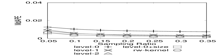
(a) Spectral Radius

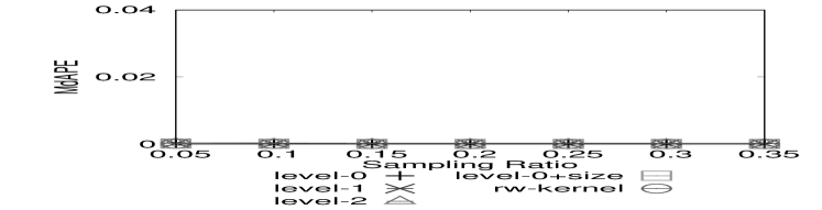
(b) Eigenvector C.

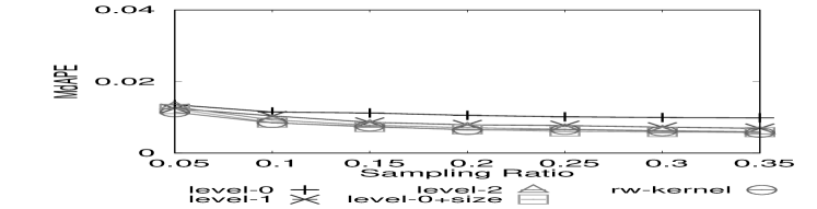
(c) Betweenness C.

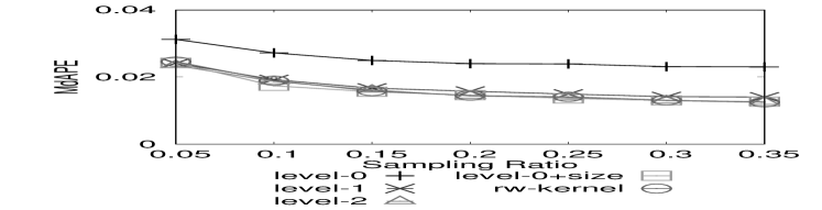
(d) Edge Betweenness C.

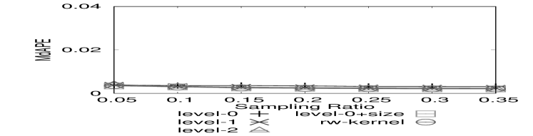
(e) Closeness C.

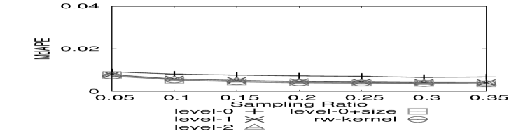
(f) PageRank

Figure 3: Similarity Metrics Comparison (AS)

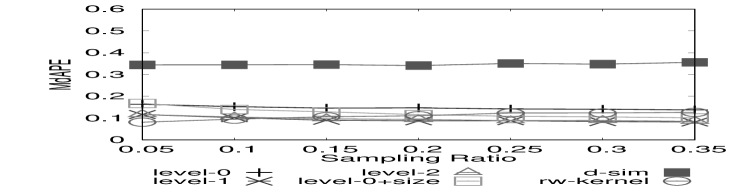
(g) Spectral Radius

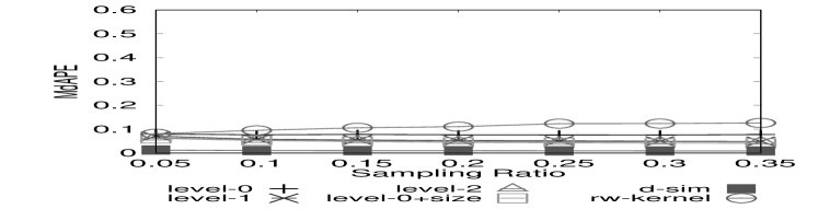
(h) Eigenvector C.

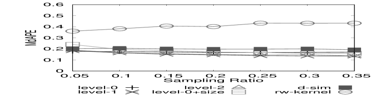
(i) Betweenness C.

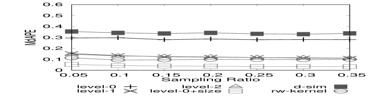
(j) Edge Betweenness C.

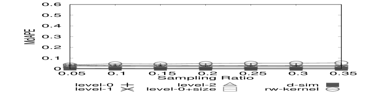
(k) Closeness C.

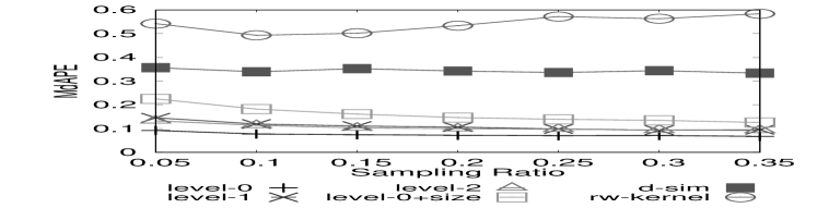
(l) PageRank

Figure 4: Similarity Metrics Comparison (TW)

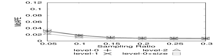
(a) Spectral Radius

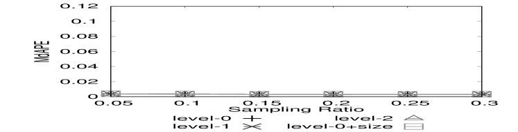
(b) Eigenvector C.

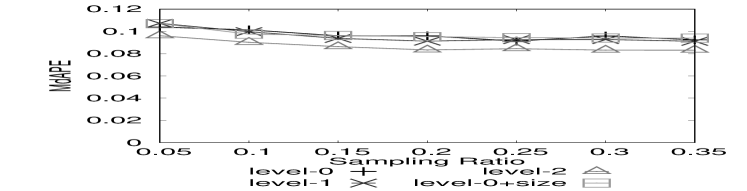
(c) Betweenness C.

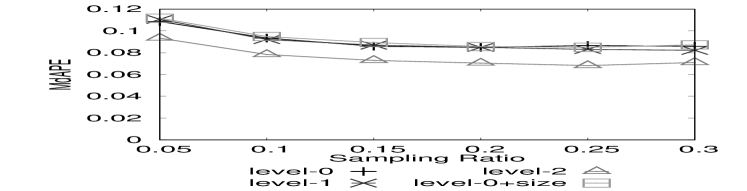
(d) Edge Betweenness C.

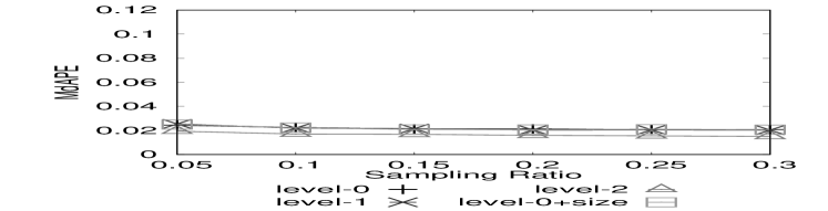
(e) Closeness C.

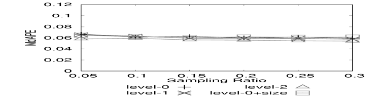
(f) PageRank

Figure 5: Similarity Metrics Comparison (BA)

$\triangleright$ Comparing Similarity Measures: The results of the similarity measure comparisons, for the AS, TW and BA datasets, are displayed in Figures 5, 5 and 5, respectively, where $MdAPE$ is used to express the modeling error. For the TW dataset we compare six similarity measures: The degree distribution + levels measure (for levels equal from 0 to 2), a combination of level-0 degree distribution with vertex count (denoted by level-0 + size), D-measure and the Random Walk Kernel based similarity measure (denoted by rw-kernel). In the cases of AS and BA we do not include D-measure, since it was not possible to compute it, for the graphs of those datasets, because of its running time. In addition for BA we do not include rw-kernel for the same reason. The results indicate the impact that the choice of similarity measure has on modeling accuracy. A more suitable to the modeled operator and detailed similarity measure is more sensitive to topology differences and can lead to better operator modeling.

Focusing on the TW dataset, we observe that in all figures, with the exception of PageRank, the degree distribution + levels similarity measure, for a number of levels, can model an operator more accurately than the simple degree distribution-based, effectively reducing the errors reported in Table 2. Indeed, the addition of more levels to the degree distribution incorporates more information about the connectivity of each vertex. This additional topological insights contribute positively to better estimate the similarity of two graphs. For instance, this allows the MdAPE error to drop from 29.5% to about 15% when utilizing a level-2 similarity for edge betweenness centrality and $p=5\%$.

Examining the modeling quality, we observe that it increases but only up to a certain point, in relation to the topology of the graphs in the dataset. For example, since TW comprises of ego graphs, all the degrees of level $>2$ are zero, since there exist no vertices with distance greater than $2$; therefore, employing more levels does not contribute any additional information about the topology of the graphs when computing their similarity.

Finally, we observe that, in specific cases, such as PageRank (Figure 3(l)), enhancing the degree distribution with degrees of more levels introduces information that is interpreted as noise during modeling. PageRank is better modeled with the simple degree distribution as a similarity measure. As such, we argue that for a given dataset and graph operator, experimentation is required to find the number of levels that give the best tradeoff between accuracy and execution time.

We next concentrate on the effect of the combination of degree distribution with vertex count in the modeling accuracy. We note that the vertex count contributes positively in the modeling of distance-related metrics while having a neutral or negative impact on degree- and spectrum-related metrics. This is attributed to the existence of, at least, a mild correlation, between vertex count and bc, ebc and cc [26]. For our least accurately approximated task, edge betweenness centrality, employing the combination of measures results in a more than 6$\times$ decrease in error.

For D-measure, our experiments show that, for distance-related metrics it performs at least as good as the degree distribution + levels similarity measures for a given level, with the notable exception of the PageRank case. On the other hand, the degree distribution can be sufficiently accurate for degree- or spectrum-related metrics. As D-measure is based on distance distributions between vertices, having good accuracy for distance-related measures is something to be expected. However, degree distribution + levels measures exhibit comparable accuracy for distance-related metrics as well. A good example of the effectiveness of D-measure is shown in the case of closeness centrality that involves all-pairs node distance information directly incorporated in D-measure as we have seen in Section 3.1. In Figure 3(k) we observe that by adding levels we get better results, vertex count contributes into even better modeling but D-measure gives better approximations. Yet, our methods’ errors are already very small (less than 3%) in this case. Considering the rw-kernel similarity measure, we observe that it performs poorly for most of the modeled operators. Although its modeling accuracy is comperable to the degree distribution + levels similarity measures for some operators, we find that for a certain level or in combination with vertex count a degree distribution-based measure has better accuracy. Notably, rw-kernel has low accuracy for degree and distance related operators while performing comperably in the case of spectrum operators.

Identifying betweenness centrality as one of the hardest operators to model accurately, we note that, for the AS and BA datasets, the approximation error is below $12\%$ and that the degree distribution + levels measures further improve on it for both datasets. Compared to TW (Fig. 5), we observe that the level-2 similarity measure provides better results for AS and BA but not TW, something we attribute to the fact that TW consists of ego graphs with their level-2 degree being equal to zero. Finally, it is expected that level-0 + size for BA to be no different than plain level-0 since all the graphs in BA have the same vertex count by construction.

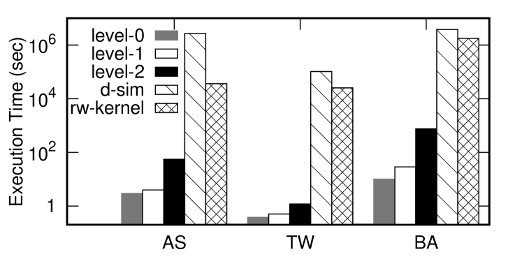
Figure 6: Execution Time (sec)

Although the above similarity measures are comparable in modeling accuracy, they are not in execution time. A comparison in computation time for different levels of the degree distribution + levels similarity measure is presented in Figure 6. In the case of D-measure, the actual execution time is presented for the TW dataset, since it was prohibitively slow to compute it for the other two datasets. For the remaining two datasets, we have computed D-measure on a random number of pairs of graphs and then projected the mean computation time to the number of comparisons performed by our method for each dataset.

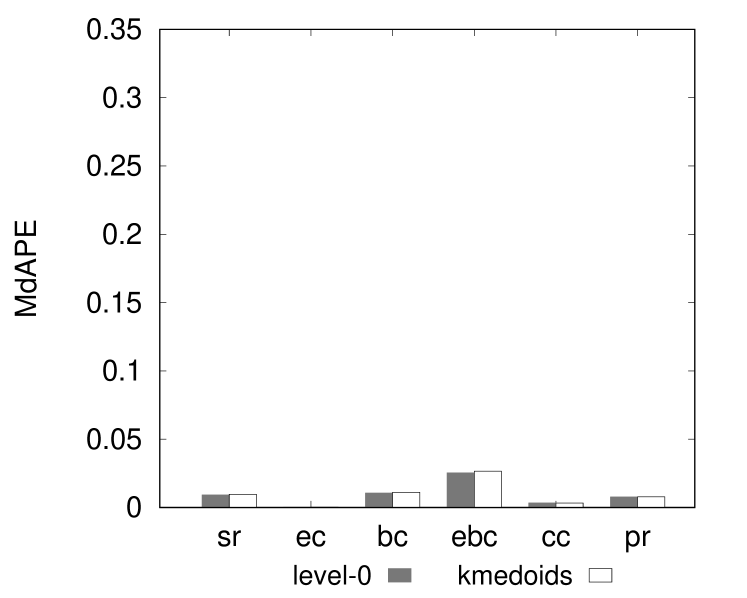
(a) AS ($p=15\%$)

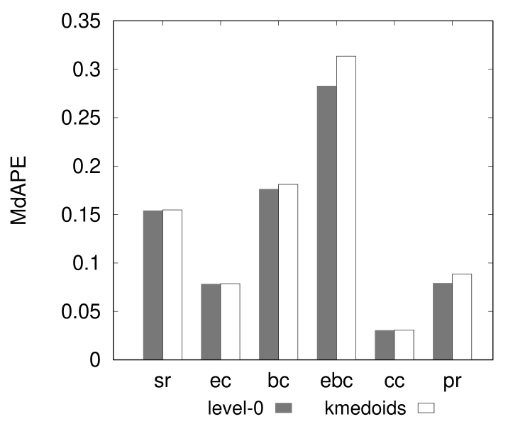
(b) TW ($p=10\%$)

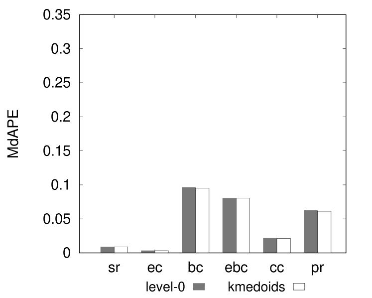
(c) BA10k ($p=3\%$)

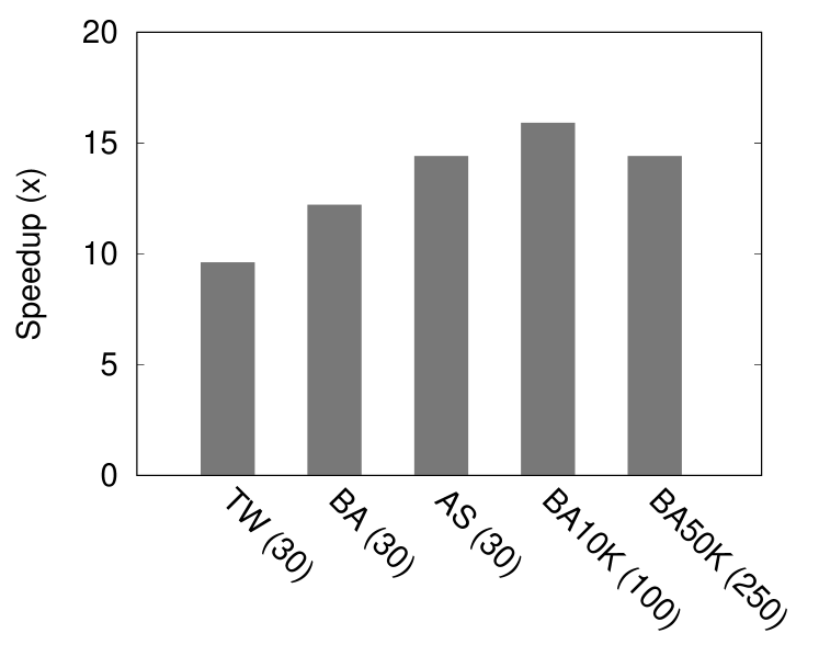
(d) Similarity Computations

Figure 7: All-Pairs Similarities vs Clustering

Our results show that the overhead from level-0 to level-1 is comparable for all the datasets. However, that is not the case for level-2. The higher the level, the more influential the degree of the vertices becomes in the execution time. Specifically, while we find level-0 to be $3.2\times$ faster than level-2 for TW, we observe that in the case of AS and BA it is $19\times$ and $76\times$ faster. The computation of the D-measure and the rw-kernel, on the other hand, are orders of magnitude slower, i.e., we find level-0 to be about 385K times faster than D-measure for the TW dataset, while it is 273K and 933K times faster for the BA and AS datasets, respectively. Given the difference in modeling quality between the presented similarity functions, we observe a clear tradeoff between quality of results and execution time in the context of our method.

$\triangleright$ Similarity Matrix Computation Speedup: In order to evaluate the effectiveness of the similarity matrix optimization we outlined in section 2.2, in Fig. 7 we present experimental results both in terms of modeling accuracy and speedup. As we aim at evaluating the scalability of our method we introduce two larger synthetic datasets BA10k and BA50k. They are both created with the same settings used for the BA dataset and contain 10k and 50k graphs respectively.

In Fig. 7(a), 7(b) and 7(c) we compare the modeling error between all-pairs similarity matrix (level-0) and clustered similarity matrix (kmedoids) for the AS, TW and BA10k datasets. As we mentioned in Section 2, we calculate MdAPE and nRMSE for a randomized $20\%$ of our datasets. For each dataset we use a sampling ratio $p$ based on the parameter $k=3$ of kNN and the number of clusters we intend to create which we set to $\sqrt{N}$. Thus, for a dataset of 10k graphs we create 100 clusters and require $300$ graph samples, therefore we set the sampling ratio to $3\%$. The graph samples are randomly chosen ensuring that we have at least $k$ from each cluster. In figure 7(d) we present speedups in the number of similarity computations performed in each of the above cases for all datasets. We observe that the clustering optimization adds at most a $3\%$ error in the case of TW while achieving a $10\times$ speedup when we use $30$ clusters. Focusing on the BA10k and BA50k datasets, we observe marginal error increases and speedups up to $15\times$. Consequently, we argue that this optimization allows our method to scale efficiently to large graph datasets.

4 Related Work

Our work relates to the actively researched areas of graph similarity, graph analytics and machine learning.

4.1 Graph Similarity

The problem of determining the degree of similarity between two graphs (or networks) has been well studied. The available techniques for quantifying graph similarity can be classified into three main categories ([29, 40]):
$\triangleright$ Graph Isomorphism - Edit Distance: Two graphs are considered similar if they are isomorphic, i.e., there is a bijection between the vertex sets of the two graphs such that two vertices of one graph are adjacent if and only if their images are also adjacent [8]. A more relaxed approach is to consider the problem of subgraph isomorphism where one graph is isomorphic to a subgraph of the other. A generalization of the graph isomorphism problem is expressed through the Edit Distance, i.e., the number of operations, such as additions or removals of edges or nodes, that have to be performed in order to transform one graph to the other [35]. The drawback of approaches in this category is that the graph isomorphism problem is hard to compute. The fastest algorithm to solve it runs in quasi-polynomial time with previous solutions being of exponential complexity [3]. Considering our method, a quasi-polynomial similarity measure is very expensive, since we have to compute all-pairs similarity scores for a given graph dataset.
$\triangleright$ Iterative Methods: This category of graph similarity algorithms is based on the idea that two vertices are similar if their neighborhoods are similar. Applying this idea iteratively over the entire graph can produce a global similarity score when the process converges. Based on this iterative approach there are algorithms like SimRank [27] or the algorithm proposed by Zager et al. [40] that compute similarities between graphs or graph nodes. Such algorithms compare graphs based on their topology, thus their performance depends on graph size. Considering our case, the efficiency of our method would depend on the size of the graphs we compare. Alternatively, we choose to map graphs to feature vectors and base our similarity scores on vector comparisons. Since the feature vectors are of low dimensionality compared to graphs, this approach is more efficient.
$\triangleright$ Feature Vector Extraction: These approaches are based on the idea that similar graphs share common properties such as degree distribution, diameter, clustering coefficient, etc. Methods in this class represent graphs as feature vectors. To assess the degree of similarity between graphs, statistical tools are used to compare their feature vectors instead. Such methods are not as computationally demanding and thus scale better. Drawing from this category of measures, in our work, we base our graph similarity computations on comparing degree distributions.
$\triangleright$ Graph Kernels: A different approach to graph similarity comes from the area of machine learning where kernel functions can be used to infer knowledge about samples. A kernel can be thought of as a measure of similarity between two objects which satisfies two mathematical properties, it is symmetric and positive semi-definite. Graph kernels are kernel functions constructed on graphs or graph nodes for comparing graphs or nodes respectively. Extensive research on this area (e.g., [20, 18]) has resulted in many kernels based on walks, paths, subgraphs, substree patterns, etc. While computationally more expensive than feature vector extraction similarity methods, they provide a good baseline for our modeling accuracy evaluation.

4.2 Graph Analytics & Machine Learning

Although graph analytics is a very thoroughly researched area, there exist few cases where machine learning techniques are used. On the subject of graph summarization, a new approach is based on node representations that are learned automatically from the neighborhood of a vertex. Such representations are a mapping of vertices to a low-dimensional space of features that aims at capturing their neighborhood structure. Works in this direction [21] focus on learning node representations and using those for graph summarization and/or compression. Node representations are also applicable in computing node or graph similarities as seen in [21] and [33]. However, we do not find works employing machine learning techniques in the field of graph mining through graph topology metric computations. Most of the research on that field focuses on approximation algorithms (e.g., [34, 15]).

5 Conclusion

As the Graph Analytics landscape evolves, an increasing number of graph operators are required to be executed over large graph datasets in order to identify those of “high interest”. To this end, we present an operator-agnostic modeling methodology which leverages similarity between graphs. This knowledge is used by a kNN classifier to model a given operator allowing scientists to predict operator output for any graph without having to actually execute the operator. We propose an intuitive, yet powerful class of similarity measures that efficiently capture graph relations. Our thorough evaluation indicates that modeling a variety of graph operators is not only possible, but it can also provide results of very high quality at considerable speedups. This is especially true when adopting a lightweight, yet highly effective similarity measure as those introduced by our work. Finally, our approach appears to present similar results to state-of-the-art similarity measures, such as D-measure, in terms of quality, but requires orders of magnitude less execution time.

References

- [1] F. J. Aherne, N. A. Thacker, and P. I. Rockett. The bhattacharyya metric as an absolute similarity measure for frequency coded data. Kybernetika, 34(4):363–368, 1998.
- [2] D. Arthur and S. Vassilvitskii. k-means++: the advantages of careful seeding. In Proceedings of the Eighteenth Annual ACM-SIAM Symposium on Discrete Algorithms, SODA 2007, New Orleans, Louisiana, USA, January 7-9, 2007, pages 1027–1035, 2007.
- [3] L. Babai. Graph isomorphism in quasipolynomial time [extended abstract]. In Proceedings of the 48th Annual ACM SIGACT Symposium on Theory of Computing, STOC 2016, Cambridge, MA, USA, June 18-21, 2016, pages 684–697, 2016.
- [4] A.-L. Barabási and R. Albert. Emergence of scaling in random networks. Science, 286(5439):509–512, 1999.
- [5] J. L. Bentley. Multidimensional binary search trees used for associative searching. Commun. ACM, 18(9):509–517, 1975.
- [6] A. Bhattacharyya. On a measure of divergence between two statistical populations defined by their probability distributions. Bulletin of Calcutta Mathematical Society, 35(1):99–109, 1943.
- [7] P. Bonacich. Power and centrality: A family of measures. American Journal of Sociology, 92(5):1170–1182, 1987.
- [8] A. Bondy and U. Murty. Graph Theory. Springer London, 2011.
- [9] G. Bounova and O. de Weck. Overview of metrics and their correlation patterns for multiple-metric topology analysis on heterogeneous graph ensembles. Phys. Rev. E, 85:016117, 2012.
- [10] U. Brandes and T. Erlebach. Network Analysis: Methodological Foundations (Lecture Notes in Computer Science). Springer-Verlag New York, Inc., 2005.
- [11] S. Brin and L. Page. The anatomy of a large-scale hypertextual web search engine. Computer Networks, 30(1-7):107–117, 1998.
- [12] T. H. Cormen, C. E. Leiserson, R. L. Rivest, and C. Stein. Introduction to Algorithms, Third Edition. The MIT Press, 2009.
- [13] G. Csardi and T. Nepusz. The igraph software package for complex network research. InterJournal, Complex Systems:1695, 2006.
- [14] L. da F. Costa, F. A. Rodrigues, G. Travieso, and P. R. V. Boas. Characterization of complex networks: A survey of measurements. Advances in Physics, 56(1):167–242, 2007.
- [15] D. Eppstein and J. Wang. Fast approximation of centrality. J. Graph Algorithms Appl., 8:39–45, 2004.
- [16] L. C. Freeman. A set of measures of centrality based on betweenness. Sociometry, 40(1):35–41, 1977.
- [17] A. Gandomi and M. Haider. Beyond the Hype. Int. J. Inf. Manag., 35(2):137–144, 2015.
- [18] T. Gärtner. A survey of kernels for structured data. SIGKDD Explorations, 5(1):49–58, 2003.
- [19] T. Gärtner, P. A. Flach, and S. Wrobel. On graph kernels: Hardness results and efficient alternatives. In Computational Learning Theory and Kernel Machines, 16th Annual Conference on Computational Learning Theory and 7th Kernel Workshop, COLT/Kernel 2003, Washington, DC, USA, August 24-27, 2003, Proceedings, pages 129–143, 2003.
- [20] S. Ghosh, N. Das, T. Gonçalves, P. Quaresma, and M. Kundu. The journey of graph kernels through two decades. Computer Science Review, 27:88–111, 2018.
- [21] A. Grover and J. Leskovec. node2vec: Scalable feature learning for networks. In Proceedings of the 22nd ACM SIGKDD International Conference on Knowledge Discovery and Data Mining, San Francisco, CA, USA, August 13-17, 2016, pages 855–864, 2016.
- [22] A. Halevy, P. Norvig, and F. Pereira. The unreasonable effectiveness of data. IEEE Intelligent Systems, 24(2):8–12, 2009.
- [23] T. Hastie, R. Tibshirani, and J. Friedman. The Elements of Statistical Learning: Data Mining, Inference, and Prediction, Second Edition. Springer New York.
- [24] J. M. Hernández and P. V. Mieghem. Classification of graph metrics. pages 1–20, 2011.
- [25] A. Jamakovic, R. E. Kooij, P. V. Mieghem, and E. R. van Dam. Robustness of networks against viruses: the role of the spectral radius. In 2006 Symposium on Communications and Vehicular Technology, pages 35–38, 2006.
- [26] A. Jamakovic and S. Uhlig. On the relationships between topological measures in real-world networks. NHM, 3(2):345–359, 2008.
- [27] G. Jeh and J. Widom. Simrank: A measure of structural-context similarity. In Proceedings of the Eighth ACM SIGKDD International Conference on Knowledge Discovery and Data Mining, pages 538–543. ACM, 2002.
- [28] L. Kaufmann and P. Rousseeuw. Clustering by means of medoids. pages 405–416, 01 1987.
- [29] D. Koutra, A. Parikh, A. Ramdas, and J. Xiang. Algorithms for graph similarity and subgraph matching. Technical Report Carnegie-Mellon-University, 2011.
- [30] J. Leskovec and A. Krevl. SNAP Datasets: Stanford large network dataset collection. http://snap.stanford.edu/data, June 2014.
- [31] J. Leskovec and R. Sosič. Snap: A general-purpose network analysis and graph-mining library. ACM Transactions on Intelligent Systems and Technology (TIST), 8(1):1, 2016.
- [32] M. E. J. Newman and M. Girvan. Finding and evaluating community structure in networks. Phys. Rev. E, 69(2):026113, 2004.
- [33] L. F. R. Ribeiro, P. H. P. Saverese, and D. R. Figueiredo. struc2vec: Learning node representations from structural identity. In Proceedings of the 23rd ACM SIGKDD International Conference on Knowledge Discovery and Data Mining, Halifax, NS, Canada, August 13 - 17, 2017, pages 385–394, 2017.
- [34] M. Riondato and E. M. Kornaropoulos. Fast approximation of betweenness centrality through sampling. Data Min. Knowl. Discov., 30(2):438–475, 2016.
- [35] A. Sanfeliu and K. Fu. A distance measure between attributed relational graphs for pattern recognition. IEEE Trans. Systems, Man, and Cybernetics, 13(3):353–362, 1983.
- [36] T. A. Schieber, L. Carpi, A. Díaz-Guilera, P. M. Pardalos, C. Masoller, and M. G. Ravetti. Quantification of network structural dissimilarities. Nature communications, 8:13928, 2017.
- [37] M. Sugiyama and K. M. Borgwardt. Halting in random walk kernels. In Advances in Neural Information Processing Systems 28: Annual Conference on Neural Information Processing Systems 2015, December 7-12, 2015, Montreal, Quebec, Canada, pages 1639–1647, 2015.
- [38] S. V. N. Vishwanathan, N. N. Schraudolph, R. Kondor, and K. M. Borgwardt. Graph kernels. Journal of Machine Learning Research, 11:1201–1242, 2010.
- [39] D. Yan, Y. Bu, Y. Tian, A. Deshpande, and J. Cheng. Big Graph Analytics Systems. In SIGMOD, 2016.
- [40] L. A. Zager and G. C. Verghese. Graph similarity scoring and matching. Appl. Math. Lett., 21(1):86–94, 2008.