Strongly gravitational lensed SNe Ia as multi-messengers: Direct test of the Friedman-Lemaître-Robertson-Walker metric

Abstract

We present a new idea of testing the validity of the Friedman-Lemaître-Robertson-Walker metric, through the multiple measurements of galactic-scale strong gravitational lensing systems with type Ia supernovae in the role of sources. Each individual lensing system will provide a model-independent measurement of the spatial curvature parameter referring only to geometrical optics independently of the matter content of the universe. This will create a valuable opportunity to test the FLRW metric directly. Our results show that with hundreds of strongly lensed SNe Ia observed by LSST, one would produce robust constraints on the spatial curvature with accuracy $\Delta\Omega_{k}=0.04$ comparable to the Planck 2015 results.

Introduction.— Friedman-Lemaître-Robertson-Walker (FLRW) metric is based on the homogeneity and isotropy of the Universe, which is supported by observations of the large-scale distribution of galaxies and the near-uniformity of the CMB temperature (Planck Collaboration XIII, 2016). Moreover, it provides the context for interpreting the observed cosmic acceleration, one of the most important issues of modern cosmology (Riess et al., 1998; Perlmutter et al., 1999). However, departure from the FLRW approximation could potentially explain the late-time cosmic acceleration (Boehm & Räsänen, 2010; Redlich et al., 2014), while growing observational data of increased precision enabled testing the robustness of the FLRW metric Clarkson et al. (2008); Shafieloo & Clarkson (2010); Mörtsell & Jönsson (2011); Sapone et al. (2014); Räsänen (2014). In particular, it was proposed that strong lensing data could provide a consistency test of the cosmic curvature (Räsänen et al., 2015; Liao et al., 2017a; Xia et al., 2017; Qi et al., 2019). However, this method makes a strong assumption based on the isotropy and homogeneity of the Universe, that the distance indicators (SNe Ia, etc.) should provide the distance information exactly applicable to galactic-scale strong lensing systems at the same redshift.

In this letter, we propose a new idea of testing the FLRW metric, through the multiple measurements of galactic-scale strong lensing systems with SNe Ia as background sources (Cao et al., 2018). Strongly gravitationally lensed SNe Ia (SGLSNe Ia thereafter), which have long been predicted in the literature long ago (Refsdal, 1964; Oguri & Marshall, 2010), had not been discovered until very recently Goobar et al. (2017); More et al. (2017). The advantage of our method is that, I) it is independent of the matter content of the Universe and its relation to space-time geometry; II) each individual lensing system provides a cosmological model-independent measurement, without any redshift correspondence from other observations. Therefore, with a sample of measurements of cosmic curvature at different sky positions, one could directly test the validity of the FLRW metric, which would be ruled out if the sum rule was violated for any pair of lensing systems. Moreover, if the sum rule was consistent with observations, this test would provide a measurement of the spatial curvature of the Universe.

Method.— Strong gravitational lensing occurs whenever the source, lens and observer are well aligned that the observer-source direction lies inside the so-called Einstein radius of the lens. We will focus on gravitational lensing caused by a galaxy-sized lens. For a SGL system with the lensing galaxy (at redshift $z_{l}$), angular separation of multiple images of the source (at redshift $z_{s}$) depends on the ratio of angular-diameter distances between lens and source $D^{A}_{l,s}$ and between observer and source $D^{A}_{s}$. Introducing dimensionless comoving distances $d_{ls}\equiv d(z_{l},z_{s})$, $d_{l}\equiv d(0,z_{l})$ and $d_{s}\equiv d(0,z_{s})$, the distance-sum-rule reads (Räsänen et al., 2015)

$$\frac{d_{ls}}{d_{s}}=\sqrt{1+\Omega_{k}d_{l}^{2}}-\frac{d_{l}}{d_{s}}\sqrt{1+\Omega_{k}d_{s}^{2}}.$$ (1)

Therefore, $\Omega_{k}$ could be directly derived from the distance ratio $d_{ls}/d_{s}$, provided the other two distances are known.

I. The angular diameter distance ratio can robustly be determined by measurement of the Einstein radius

$$\theta_{E}=\left(\frac{4GM_{E}}{c^{2}}\frac{D^{A}_{ls}}{D^{A}_{l}D^{A}_{s}}\right)^{1/2}$$ (2)

where $M_{E}$ is the mass enclosed in the cylinder of radius equal to $\theta_{E}$. We assume the spherically symmetric power-law mass distribution $\rho\sim r^{-\gamma}$, commonly used in studies of lensing caused by early-type galaxies (Treu et al., 2006; Li et al., 2016; Ma et al., 2019). After solving the spherical Jeans equation (Koopmans et al., 2005), assuming that stellar and total mass distributions follow the same power-law and velocity anisotropy vanishes, one obtains

$$\frac{d_{ls}}{d_{s}}=\frac{D^{A}_{ls}}{D^{A}_{s}}=\frac{\theta_{E}}{4\pi}\frac{c^{2}}{\sigma_{ap}^{2}}\left(\frac{\theta_{E}}{\theta_{ap}}\right)^{\gamma-2}f(\gamma,M_{E})^{-1}$$ (3)

where $f(\gamma,M_{E})$ is a function of the radial mass profile slope and $\sigma_{ap}$ is the luminosity averaged line-of-sight velocity dispersion inside the aperture $\theta_{ap}$ Cao et al. (2012, 2015).

II. Light rays from multiple images of the lensed source need different time to complete their travel along different paths and experience different Shapiro delays. Accurate observations of photometric light curves of the SNe Ia images $\bm{\theta}_{i}$ and $\bm{\theta}_{j}$ will provide time delays (Courbin et al., 2011), which are directly related to the lens potential as well as the mutual distances in the lensing system Treu et al. (2010)

$$\Delta t_{i,j}=\frac{D_{\mathrm{\Delta t}}(1+z_{\mathrm{l}})}{c}\Delta\phi_{i,j},$$ (4)

where the Fermat potential difference $\Delta\phi_{i,j}=[(\bm{\theta}_{i}-\bm{\beta})^{2}/2-\psi(\bm{\theta}_{i})-(\bm{\theta}_{j}-\bm{\beta})^{2}/2+\psi(\bm{\theta}_{j})]$ depends on the source position $\bm{\beta}$ and the two-dimensional lensing potential $\psi$ satisfies the corresponding Poisson Equation: $\nabla^{2}\psi=2\kappa$, where $\kappa$ is the surface mass density of the deflector in units of the critical density. The so-called time-delay distance introduced in Eq. (4) can be expressed as

$$D_{\mathrm{\Delta t}}\equiv\frac{D^{A}_{\mathrm{l}}D^{A}_{\mathrm{s}}}{D^{A}_{\mathrm{ls}}}=\frac{c}{1+z_{l}}\frac{\Delta t_{i,j}}{\Delta\phi_{i,j}},$$ (5)

From measurements of $\Delta t_{i,j}$ and $\Delta\phi_{i,j}$ providing the time-delay distance, combined with the distance ratio $D^{A}_{ls}/D^{A}_{s}$, one gets the distance

$$D_{l}=(1+z_{l})D_{\mathrm{\Delta t}}\frac{D^{A}_{ls}}{D^{A}_{s}}.$$ (6)

III. SNe Ia can be calibrated as standard candles providing luminosity distances $D^{L}_{s}$ through their distance moduli $\mu_{D}=m_{X}-M_{B}-K_{BX}$ (Qi et al., 2018), where $m_{X}$ is the peak apparent magnitude in the filter $X$, $M_{B}$ is its rest-frame B-band absolute magnitude, and $K_{BX}$ denotes the cross-filter K-correction (Kim et al., 1996). In our context, the unlensed SN Ia flux should be scaled up by a magnification factor $\mu$ due to gravitational lensing appropriately. Therefore, the comoving distance from the observer to the source is

$$D_{s}=\frac{10^{(\mu_{D}+2.5log\mu)/5-5}}{1+z_{s}}(Mpc).$$ (7)

Now one is able to determine

$$\Omega_{k}(z_{l},z_{s})=\frac{d_{l}^{4}+d_{s}^{4}+d_{ls}^{4}-2d_{l}^{2}d_{s}^{2}-2d_{l}^{2}d_{ls}^{2}-2d_{s}^{2}d_{ls}^{2}}{4d_{l}^{2}d_{s}^{2}d_{ls}^{2}}$$ (8)

in which the dimensionless comoving distances $d$ are related to the comoving distances $D$ as $D=cd/H_{0}$. This function is general, but in the FLRW space-time it should be equal to the present value of the spatial curvature parameter $\Omega_{k,0}$ and thus should give the same result for any pair of source and lens. Due to Strong covariance between $d_{l}$, $d_{s}$, and $d_{ls}$, instead of propagating distance uncertainties, we use Monte-Carlo simulation to project uncertainties in the lens mass profile, time delays, Fermat potential difference, and the magnification effect onto the final uncertainty of $\Omega_{k}(z_{l},z_{s})$.

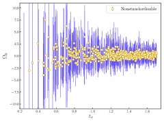
Figure 1: An example of the simulated measurements of $\Omega_{k}$ from future observations of SGLSNe Ia: without and with the effect of microlensing. The blue lines denote the associated error bars (68.3% C.L.) of $\Omega_{k}$ when all the uncertainties are included.

	$\delta\theta_{E}$	$\delta\sigma_{ap}$	$\delta\gamma$
Multiple images	1%	5%	1%
	$\delta\Delta t$	$\delta\Delta t$ (ML)	$\delta\Delta\psi$	$\delta\Delta\psi$ (LOS)
Time delay	1%	1%	$\propto(\delta\theta_{E},\delta\gamma)$	1%
	$\Delta\mu_{D}(sta)$	$\Delta\mu_{D}$ (ML)	$\delta\mu$	$\Delta\mu_{D}(sys)$
Lensed SNe Ia	$\sigma_{stat}$	0.70 mag	$\propto(\delta\theta_{E},\delta\gamma)$	$\sigma_{sys}$

Table 1: Uncertainties of contributing to the uncertainty of $\Omega_{k}(z_{l},z_{s})$ measurement (ML and LOS correspond to the microlensing effect and light-of-sight contamination, respectively). Concerning the Fermat potential and SNe Ia images magnifications by the lensing galaxy potential, relevant uncertainties were simulated by propagating uncertainties of $\theta_{E}$ and $\gamma$.

Simulated data.— Recent analysis (Goldstein & Nugent, 2017) revealed that the LSST can discover up to 650 multiply imaged SNe Ia in a 10 year $z$-band search. Following Collett (2015), we simulated a realistic population of SGLSNe Ia lensed by early-type galaxies, assuming distributions of velocity dispersions and Einstein radii similar to the SL2S sample Sonnenfeld et al. (2013a). The velocity dispersion function of the lenses in the local Universe follows the modified Schechter function Choi et al. (2007); Cao & Zhu (2012). The population of strong lenses is dominated by galaxies with velocity dispersion of $\sigma_{ap}=210\pm 50$ km/s, while the lens redshift distribution is well approximated by a Gaussian with mean 0.40. Although discovering strong lenses in future surveys will require the development of new methods and algorithms, we are confident that the simulated population of lenses is a good representation of what the future LSST survey might yield Collett (2015). In our fiducial model, the average logaritmic density slope is modeled as $\gamma=2.09$ with 10% intrinsic scatter, the results from SLACS strong-lens early-type galaxies with direct total-mass and stellar-velocity dispersion measurements Koopmans et al. (2009). Then we performed a Monte Carlo simulation to create the lensed SNe Ia sample. In each simulation, there were 650 type Ia supernova covering the redshift range of $0.00<z\leq 1.70$. When calculating the sampling distribution (number density) of the SNe Ia population, we adopted the redshift-dependent SNe Ia rate from Sullivan et al. (2000). More specifically, in our model of the SNe Ia population, we took the redshift distribution of multiply imaged SNe Ia detectable in a 10 year LSST z-band search Goldstein & Nugent (2017), which furthermore constituted the differential rates of lensed SNe Ia events as a function of $z_{s}$. For each lensed SNe Ia, following the suggestion of Goldstein & Nugent (2017), the peak rest-frame $M_{B}$ was assumed to be -19.3, while the cross-filter $K$-corrections were computed from the one-component SNe Ia spectral template Nugent et al. (2002).

I. For a specific SGL system observed with HST-like image quality, the state-of-the-art lens modeling techniques (Suyu et al., 2010, 2012) and kinematic modeling methods (Auger et al., 2010; Sonnenfeld et al., 2012) enable high precision inference of $M_{E}$, which can be measured to within 1-2% including all random and systematic uncertainties (Treu et al., 2010). Following the analysis of Collett & Cunnington (2016), fractional uncertainties of the observed velocity dispersion and the Einstein radius are 5% and 1%, respectively. Although the line-of-sight contamination might introduce 3% uncertainties (Hilbert et al., 2009), this systematics might be reduced to 1% in future strong lensing surveys. Recent analysis of the SL2S lens sample demonstrated that the total mass-density slope $\gamma$ inside the Einstein radius can be determined with 5% accuracy (Ruff et al., 2011; Sonnenfeld et al., 2013b). However, the inclusion of time delays can reduce this uncertainty to 1% (Wucknitz et al., 2004).

II. Four sources of uncertainty are included in our simulation of time-delay measurements: $\Delta t$ measurement itself, the effect of microlensing, uncertainty of Fermat potential determination and line of sight contamination. SNe Ia have many advantages over AGNs and quasars (Goldstein & Nugent, 2017), where the new curve shifting algorithms (Tewes et al., 2013a) enable $\Delta t$ measurements with 3% accuracy (Fassnacht et al., 2002; Tewes et al., 2013b; Liao et al., 2015). Time delays measured with lensed SNe Ia are supposed to be very accurate due to the exceptionally well-characterized spectral sequences and relatively small variation in quickly evolving light curve shapes and color (Nugent et al., 2002; Pereira et al., 2013). We assumed $\Delta t$ uncertainty of 1%, which seems reasonable. Next, the microlensing generated by stars in lensing galaxy, may significantly magnify lensed supernovae (Dobler & Keeton, 2006; Bagherpour et al., 2006). Concerning LSST, the distribution of absolute time delay error due to microlensing is unbiased at the sub-percent level with color curve observations in the achromatic phase Goldstein et al. (2018). Therefore, an additional 1% uncertainty of $\Delta t$ is added for SGLSNe Ia in which the microlensing is significant. The uncertainty of the Fermat potential difference is simulated from the lens mass profile and the Einstein radius uncertainties (Suyu et al., 2013). In a system with the lensed SN Ia image quality typical to the HST observations $\sim 3\%$ precision on the Fermat potential difference (Suyu et al., 2016) can be achieved. Finally, another 1% uncertainty of $\Delta\psi$ will be considered due to LOS effects (Liao et al., 2017b).

III. Three sources of uncertainties are included in our simulation of SGLSNe Ia. Following the strategy of (Spergel et al., 2015), the distance precision per SNe is $\sigma^{2}_{\rm stat}=\sigma^{2}_{\rm meas}+\sigma^{2}_{\rm int}+\sigma^{2}_{\rm lens}$ (Hounsell et al., 2017), with the mean uncertainty $\sigma_{\rm meas}=0.08$ mag, the intrinsic scatter uncertainty $\sigma_{\rm int}=0.09$ mag, and the lensing uncertainty due to the LOS mass distribution $\sigma_{\rm lens}=0.07\times z$ mag (Holz & Hughes, 2005; Jönsson et al., 2010). Moreover, the total systematic uncertainty is modeled as $\sigma_{sys}=0.01(1+z)/1.8~{}\rm{(mag)}$, which is assumed to increase with redshift (Hounsell et al., 2017). It should be stressed that the derivation of such systematic uncertainty is based on an uncorrelated SNe Ia sample, while there are known systematics contradicting this assumption (e.g., uncertainties related to calibration and SNe Ia color are correlated across a wide redshift range). The correlation between different SNe Ia might constitute an important systematic error in our $\Omega_{k}$ measurements. The statistical and systematic uncertainty are combined to produce the total uncertainty as $\sigma^{2}_{tot}=\sigma^{2}_{stat}+\sigma^{2}_{sys}$. Being standardizable candles, SGLSNe Ia can be used to assess the lensing magnification factor $\mu$ directly (Oguri & Kawano, 2003) by solving the lens equation using glafic (Oguri, 2010b). We explicitly considered that uncertainty of $\mu$ is related to uncertainties of $\gamma$ and $\theta_{E}$ (Suyu et al., 2013). Finally, only 22% of the 650 SGLSNe Ia discovered by LSST will be standardisable, due to the microlensing effect (Foxley-Marrable et al., 2018). Lensed images are standardisable in regions of low convergence, shear and stellar density (especially the outer image of an asymmetric double for lenses with large $\theta_{E}$). Therefore an additional uncertainty $\sim 0.70$ mag should be considered for the remaining 78% of SGLSNe Ia Yahalomi et al. (2017), especially in quadruple image systems, symmetric doubles and small Einstein radii lenses. All images are used to determine $\mu$ and SNe Ia distances. Table I lists the relative uncertainties of factors contributing to the accuracy of $\Omega_{k}(z_{l},z_{s})$ measurements.

We summarize the main route of our method as follows. There are three levels of random realizations that need to be simulated separately: 1) Monte Carlo simulation of the strong lensing systems; 2) the statistical errors that are independent for each lensing system; and 3) the systematic errors whose realizations are common for all systems. Specifically, in this analysis, the total systematic uncertainty is considered in the corrected SNe Ia distances, which is modeled as $\mu_{D}(sys)=0.01(1+z)/1.8~{}\rm{(mag)}$ (Hounsell et al., 2017). With the combination of these different layers of randomness, we use Monte-Carlo simulation to project the statistical uncertainties of the observables of $\gamma$, $\theta_{E}$, $\theta_{ap}$, $\Delta t$, and $\mu_{D}$, as well as the systematic uncertainty of the SNe Ia distances ($\mu_{D}$) onto the final uncertainty of $\Omega_{k}$. In order to guarantee the reliability of our results, we realize $10^{3}$ random mock data sets and apply the above algorithm to each of them.

Figure 2: Upper panel: simulated measurements of $\Omega_{k}$ divided into $z_{s}$ bins and summarized as weighted means with corresponding standard deviations. Lower panel: inverse variance weighted mean of $\Omega_{k}$ achievable from SGLSNe Ia in comparison to CMB+BAO constraints.

Constraint results.— Assuming that parameters whose uncertainties listed in Table I follow the Gaussian distribution, we simulated two sets of realistic lensed SNe Ia with and without considering the effect of microlensing. Concerning the error budget applied in this paper, one should clarify that the objective of the work is to determine uncertainties in $\Omega_{k}$ for a survey. However, in each of the $10^{3}$ Monte Carlo simulations, new surveys with independent sets of SGLSNe Ia systems are realized, which indicates that the uncertainties inherent in having one survey with one realization of SGLSNe Ia systems are underestimated. Moreover, since all of these SNe Ia are strongly lensed, the lensing dispersion of $\mu_{D}$ is also correlated with the other parameters. Therefore, in this analysis, we combined the error budget assuming zero measurement uncertainty and that assuming zero per-object intrinsic dispersion (the intrinsic magnitudes dispersion of $\mu_{D}$). An example of the simulation is shown in Fig. 1 (based on one realization of SGLSNe Ia sample with one realization of statistical and systematic errors), which were repeated $10^{3}$ times to produce the statistical results shown in Figs. 2-3 (based on $10^{3}$ realizations of SGLSNe Ia sample with $10^{3}$ realizations of statistical and systematic errors). Turning to the mock SGLSNe Ia catalogue of (Goldstein & Nugent, 2017), only 22% of the full sample discovered by LSST will be standardisable. Such conclusion is consistent with the predicted relation between the standardisable fraction and Einstein radius assuming the Salpeter IMF (Foxley-Marrable et al., 2018), which implies that 90% of the source plane with $\theta_{E}\geq 1"$ is standardisable. In our simulated data, the mean Einstein radius for standardisable SGLSNe Ia is 1.5”, compared to 0.73” for SGLSNe Ia unsuitable to be standard candles. The mean time delay for standardisable LSST SGLSNe Ia is 71 days, compared to 36 days for non-standardisable ones. Are these measurements sufficient enough to detect possible deviation from FLRW metric? As can be seen in Fig. 1, relatively low precision of individual $\Omega_{k}(z_{l},z_{s})$ measurements, especially in low-redshift SNe Ia, makes it very difficult to be competitive. However, at higher redshifts one would be able to find different $\Omega_{k}(z_{l},z_{s})$ in different pairs of $(z_{l},z_{s})$, which could indicate that light propagation on large scales was affected by departures from the FLRW metric.

Is it possible to achieve a stringent measurement of the spatial curvature from a statistical sample of SGLSNe Ia? One should be very careful to the bias induced by the $\Omega_{k}$ measurements with large uncertainties. The most straightforward way of summarizing multiple measurements is inverse variance weighting (Zheng et al., 2016; Denissenya et al., 2018)

$$\begin{array}[]{l}\bar{\Omega_{k}}=\frac{\sum\left(\Omega_{k,i}/\sigma^{2}_{\Omega_{k,i}}\right)}{\sum 1/\sigma^{2}_{\Omega_{k,i}}},\\ \sigma^{2}_{\bar{\Omega_{k}}}=\frac{1}{\sum 1/\sigma^{2}_{\Omega_{k,i}}},\end{array}$$ (9)

where $\bar{\Omega_{k}}$ stands for the weighted mean of cosmic curvature with uncertainty $\sigma_{\bar{\Omega_{k}}}$. In order to get a better feeling of the bias inherent to the $\Omega_{k}(z_{l},z_{s})$ observable due to its complex nonlinear dependence on observable quantities, we subdivided simulated 650 data points into 8 redshift bins of width $\Delta z=0.2$. The result is shown in Fig. 2 where weighted means and corresponding standard deviations are shown for each bin, allowing a direct check of its predicted constancy with redshift. It is worth noticing that, although there is a bias in the weighted mean $\Omega_{k}$ with large uncertainties at low-redshifts, the mean value of the cosmic curvature is still located within the error bar (68.3% C. L.). A thorough discussion of such biases and a proposal for remedy was given in Denissenya et al. (2018). However, the observational setting discussed in this interesting and important paper was different from ours. Second panel of Fig. 2 shows the constraints (inverse variance weighted mean) achievable from the full SGLSNe Ia in comparison to CMB+BAO model-dependent constraints.

Using only standardizable SNe Ia we are able to constrain the cosmic curvature parameter with the precision of $\Delta\Omega_{k}=0.13$. The remaining $78\%$ corrected for the microlensing effect, give $\Delta\Omega_{k}=0.09$. Finally, the full sample of 650 lensed SNe Ia will improve the constraint to $\Delta\Omega_{k}=0.08$. Our method might perform better, with the Chabrier IMF more lensed SNe Ia can be classified as standard candles: lenses with smaller Einstein radius ($\theta_{E}\sim 0.4"$) can have a source plane which is 90% standardisable (Foxley-Marrable et al., 2018). Namely, with 650 simulated SGLSNe Ia, the cosmic curvature parameter can be determined to $\Delta\Omega_{k}=0.04$, which is comparable to that of the power spectra (TT,TE,EE+lowP) from the Planck 2015 results (Planck Collaboration XIII, 2016). Therefore, by comparing spatial curvature from SGLSNe Ia with the constraints obtained from CMB, one will be able to test the validity of the FLRW metric. The curvature determined from CMB and BAO is impressively consistent with flat universe $\Delta\Omega_{k}=0.005$ (Planck Collaboration XIII, 2016) and future CMB missions and BAO surveys (CORE + DESI) are expected to constrain curvature at $\Delta\Omega_{k}=0.0008$ Di Valentino et al. (2018). We emphasize an alternative nature of our method. Stringent constraints could be obtained through the CMB+BAO combined analysis (see Fig. 2) in a model dependent way. However, assessment of the spatial curvature based on local objects like strongly lensed supernovae would be of paramount importance being able to probe deviations from the FLRW metric caused by the structure formation, which is inaccessible to the tools like CMB, BAO, and the interpolations of redshift differences detected from galaxy redshift surveys Alam et al. (2015); Laureijs et al. (2011).

Figure 3: Inferred $\Omega_{k}$ parameter as a function of the number of SGLSNe Ia, with the prediction of a silent universe added for comparison.

Is it possible to confirm or falsify alternative approaches like the back-reaction from inhomogeneities? Bolejko (2017a, b) examined the so-called silent universe in which the back-reaction of inhomogeneities was taken into account. The most striking conclusion of these works is the emergence of spatial curvature in the low redshift universe: $\Omega_{k}=0.15^{+0.04}_{-0.03}$ (95% confidence level). Note studies of the local universe encompass a region with redshifts approximately less than 0.1, where there is a linear Hubble Flow and low redshift-data (SNe Ia) can be observed in most detail. It is interesting to see if our method can be used to test this prediction. Fig. 3 shows the precision of the curvature parameter assessment as a function of SGLSNe Ia sample size. One can see that, even with 50 SGLSNe Ia one can effectively differentiate between the silent universe and the concordance $\Lambda$CDM cosmology, which means that the phenomenon of emerging curvature will soon be directly testable with observational data and furthermore strengthens the probative power of our method to inspire new observing programs or theoretical work in the moderate future.

In order to implement our method, dedicated observations including spectroscopic redshift measurements of the lens and the source, velocity dispersion of the lens, higher angular resolution imaging to measure the Einstein radius, and dedicated campaigns to measure time delays would be necessary. Obtaining these data for a sample of several hundreds of SGLSNe Ia would require substantial follow-up efforts, similar to that made in strong gravitational lens ESO 325-G004 (Collett et al., 2018). Despite of these difficulties, one may expect that multiple measurements of SGLSNe Ia can become an independent alternative to current probes Cao et al. (2017b, c); Ma et al. (2017); Qi et al. (2017); Xu et al. (2018); Cao et al. (2019), useful for more precise empirical studies of the FLRW metric. Finally, concerning the probative power of our method, the methodology proposed in this paper might be extended to strongly lensed gravitational wave (GW) events detected by aLIGO and the proposed ET (Li et al., 2018). Given the wealth of available gravitational lensing data in EM and GW domain, we may be optimistic about detecting possible deviation from the FLRW metric within our observational volume in the future. Such accurate model-independent measurements of the FLRW metric can become a milestone in precision cosmology.

Acknowledgements.— We are grateful to Paul L. Schechter for useful discussions. This work was supported by National Key R&D Program of China No. 2017YFA0402600, the National Natural Science Foundation of China under Grants Nos. 11690023, 11373014, and 11633001, Beijing Talents Fund of Organization Department of Beijing Municipal Committee of the CPC, the Strategic Priority Research Program of the Chinese Academy of Sciences, Grant No. XDB23000000, the Interdiscipline Research Funds of Beijing Normal University, and the Opening Project of Key Laboratory of Computational Astrophysics, National Astronomical Observatories, Chinese Academy of Sciences. J.-Z. Qi was supported by China Postdoctoral Science Foundation under Grant No. 2017M620661, and the Fundamental Research Funds for the Central Universities N180503014. This research was also partly supported by the Poland- China Scientific & Technological Cooperation Committee Project No. 35-4. M. Biesiada was supported by Foreign Talent Introducing Project and Special Fund Support of Foreign Knowledge Introducing Project in China.

References

- Planck Collaboration XIII (2016) Ade, P. A. R., Aghanim, N., Arnaud, M., et al. 2016, A&A, 594, A13
- Riess et al. (1998) Riess, A. G., et al. 1998, AJ, 116, 1009
- Perlmutter et al. (1999) Perlmutter, S., et al. 1999, ApJ, 517, 567
- Redlich et al. (2014) Redlich, M., et al. 2014, A&A, 570, A63
- Boehm & Räsänen (2010) Boehm, C., & Räsänen, S. 2013, JCAP, 09, 003
- Clarkson et al. (2008) Clarkson, C., et al. 2008, PRL, 101, 011301
- Shafieloo & Clarkson (2010) Shafieloo, A., & Clarkson, C. 2010, PRD, 81, 083537
- Mörtsell & Jönsson (2011) Mörtsell, E., & Jönsson, J. 2011, [arXiv:1102.4485]
- Sapone et al. (2014) Sapone, D., et al. 2014, PRD, 90, 023012
- Räsänen (2014) Räsänen, S. 2014, JCAP, 03, 035
- Räsänen et al. (2015) Räsänen, S., et al. 2015, PRL, 115, 101301
- Liao et al. (2017a) Liao, K., et al. 2017a, ApJ, 839, 70
- Xia et al. (2017) Xia, J.-Q., Yu, H., Wang, G.-J., et al. 2017, ApJ, 834, 75
- Qi et al. (2019) Qi, J.-Z., et al. 2019, MNRAS, 483, 1104
- Cao et al. (2018) Cao, S., et al. 2018, ApJ, 867, 50
- Refsdal (1964) Refsdal, S. 1964, MNRAS, 128, 307
- Oguri & Marshall (2010) Oguri, M. & Marshall, P. J. 2010, MNRAS, 405, 2579
- Goobar et al. (2017) Goobar, A., Amanullah, R., Kulkarni, S. R., et al. 2017, Science, 356, 291
- More et al. (2017) More, A., et al. 2017, ApJL, 835, L25
- Treu et al. (2006) Treu, T., et al. 2006b, ApJ, 650, 1219
- Li et al. (2016) Li, X. L., et al. 2016, RAA, 16, 84
- Ma et al. (2019) Ma, Y.-B., et al. 2019, EPJC, 79, 121
- Koopmans et al. (2005) Koopmans L.V.E. 2005, Proceedings of XXIst IAP Colloquium, “Mass Profiles & Shapes of Cosmological Structures” (Paris, 4-9 July 2005), eds G. A. Mamon, F. Combes, C. Deffayet, B. Fort (Paris: EDP Sciences) [astro-ph/0511121]
- Cao et al. (2012) Cao, S., et al. 2012, JCAP, 03, 016
- Cao et al. (2015) Cao, S., et al. 2015, ApJ, 806, 66
- Courbin et al. (2011) Courbin, F., et al. 2011, A&A, 536, A53
- Treu et al. (2010) Treu, T. et al. 2010, ARA&A, 48, 87
- Qi et al. (2018) Qi, J. Z., et al. 2018, RAA, 18, 66
- Kim et al. (1996) Kim, A., Goobar, A., & Perlmutter, S. 1996, PASP, 108, 190
- Goldstein & Nugent (2017) Goldstein, D. A. & Nugent, P. E. 2017, ApJL, 834, L5
- Collett (2015) Collett, T. E. 2015, ApJ, 811, 20
- Sonnenfeld et al. (2013a) Sonnenfeld, A., Treu, T., Gavazzi, R., et al. 2013a, ApJ, 777, 98
- Choi et al. (2007) Choi, Y.-Y., et al. 2007, ApJ, 658, 884
- Cao & Zhu (2012) Cao, S., & Zhu, Z.-H. 20112, A&A, 538, A43
- Koopmans et al. (2009) Koopmans, L. V. E., et al. 2009, ApJL, 703, L51
- Sullivan et al. (2000) Sullivan, M., Ellis, R., Nugent, P., Smail, I., & Madau, P. 2000, MNRAS, 31
- Nugent et al. (2002) Nugent, P., Kim, A., & Perlmutter, S. 2002, PASP, 114, 803
- Suyu et al. (2010) Suyu, S. H., et al. 2010, ApJ, 711, 201
- Suyu et al. (2012) Suyu, S. H., et al. 2012, ApJ, 750, 10
- Auger et al. (2010) Auger, M. W., et al. 2010, ApJ, 724, 511
- Sonnenfeld et al. (2012) Sonnenfeld, A., et al. 2012, ApJ, 752, 163
- Collett & Cunnington (2016) Collett, T. E. & Cunnington, S. D. 2016, MNRAS, 462, 3255
- Hilbert et al. (2009) Hilbert, S., et al. 2009, A&A, 499, 31
- Ruff et al. (2011) Ruff, A., et al. 2011, ApJ, 727, 96
- Sonnenfeld et al. (2013b) Sonnenfeld, A., Gavazzi, R., Suyu, S.H., Treu, T., Marshall, P.J. 2013b, ApJ, 777, 97
- Wucknitz et al. (2004) Wucknitz, O., Biggs, A. D, Browne, I. W. A. 2004, MNRAS, 349, 14
- Tewes et al. (2013a) Tewes, M., Courbin, F., Meylan, G. 2013a, A&A, 553, A120
- Fassnacht et al. (2002) Fassnacht, C. D., et al. 2002, ApJ, 581, 823
- Tewes et al. (2013b) Tewes, M., et al. 2013b, A&A, 556, A22
- Liao et al. (2015) Liao, K., et al. 2015, ApJ, 800, 11
- Pereira et al. (2013) Pereira, R., Thomas, R. C., Aldering, G., et al. 2013, A&A, 554, A27
- Dobler & Keeton (2006) Dobler, G., & Keeton, C. R. 2006, ApJ, 653, 1391
- Bagherpour et al. (2006) Bagherpour, H., Branch, D., & Kantowski, R. 2006, ApJ, 638, 946
- Goldstein et al. (2018) Goldstein, D. A., et al. 2018, ApJ, 855, 22
- Suyu et al. (2013) Suyu, S. H., et al. 2014, ApJ Lett, 788, L35
- Suyu et al. (2016) Suyu, S. H., et al., 2017, MNRAS, 468, 2590
- Liao et al. (2017b) Liao, K., Fan, X.-L., Ding, X., Biesiada, M. & Zhu Z.-H., 2017b, Nature Communications, 8, 1148
- Spergel et al. (2015) Spergel, D., et al., 2015, [arXiv:1503.03757]
- Hounsell et al. (2017) Hounsell, R., et al. 2017, [arXiv:1702.01747v1]
- Holz & Hughes (2005) Holz, D. E., & Hughes, S. A., 2005, ApJ, 629, 15
- Jönsson et al. (2010) Jönsson, J., et al. 2010, MNRAS, 405, 535
- Oguri & Kawano (2003) Oguri, M., & Kawano, Y. 2003, MNRAS, 338, L25
- Oguri (2010b) Oguri, M. 2010, PASJ, 62, 1017
- Foxley-Marrable et al. (2018) Foxley-Marrable, M., et al. 2018, [arXiv:1802.07738]
- Yahalomi et al. (2017) Yahalomi, D., et al. 2017, [arXiv:1711.07919]
- Zheng et al. (2016) Zheng, X. G., et al. 2016, ApJ, 825, 17
- Denissenya et al. (2018) Denissenya, M., Linder, E.V., & Shafieloo, A. 2018, JCAP, 03, 041
- Di Valentino et al. (2018) Di Valentino, E., et al. 2018, JCAP, 04, 017
- Alam et al. (2015) Alam, S., et al. 2015, ApJS, 219, 12
- Laureijs et al. (2011) Laureijs, R., et al., ”Euclid Definition Study Report”, arXiv:1110.3193
- Bolejko (2017a) Bolejko, K. 2017a, [arXiv:1707.01800]
- Bolejko (2017b) Bolejko, K. 2017b, Class. Quantum Grav., 35, 024003
- Collett et al. (2018) Collett, T. E., et al. 2018, Science, 360, 1342
- Cao et al. (2017b) Cao, S., Biesiada, M., Jackson, J., Zheng, X. & Zhu Z.-H. 2017b, JCAP, 02, 012
- Cao et al. (2017c) Cao, S., Zheng X., Biesiada M., Qi J., Chen Y. & Zhu Z.-H. 2017c, A&A, 606, A15
- Ma et al. (2017) Ma, Y.-B., et al. 2017, EPJC, 77, 891
- Qi et al. (2017) Qi, J. Z., et al. 2017, EPJC, 77, 02
- Xu et al. (2018) Xu, T. P., et al. 2018, JCAP, 06, 042
- Cao et al. (2019) Cao, S., et al. 2019, Physics of the Dark Universe, 24, 100274
- Li et al. (2018) Li, S. S., et al. 2018, MNRAS, 476, 2220