Scalar Casimir densities and forces for parallel plates
in cosmic string spacetime

Abstract

We analyze the Green function, the Casimir densities and forces associated with a massive scalar quantum field confined between two parallel plates in a higher dimensional cosmic string spacetime. The plates are placed orthogonal to the string and the field obeys the Robin boundary conditions on them. The boundary-induced contributions are explicitly extracted in the vacuum expectation values (VEVs) of the field squared and of the energy-momentum tensor for both the single plate and two plates geometries. The VEV of the energy-momentum tensor, in additional to the diagonal components, contains an off-diagonal component corresponding to the shear stress. The latter vanishes on the plates in special cases of Dirichlet and Neumann boundary conditions. For points outside the string core the topological contributions in the VEVs are finite on the plates. Near the string the VEVs are dominated by the boundary-free part, whereas at large distances the boundary-induced contributions dominate. Due to the nonzero off-diagonal component of the vacuum energy-momentum tensor, in addition to the normal component, the Casimir forces have nonzero component parallel to the boundary (shear force). Unlike the problem on the Minkowski bulk, the normal forces acting on the separate plates, in general, do not coincide if the corresponding Robin coefficients are different. Another difference is that in the presence of the cosmic string the Casimir forces for Dirichlet and Neumann boundary conditions differ. For Dirichlet boundary condition the normal Casimir force does not depend on the curvature coupling parameter. This is not the case for other boundary conditions. A new qualitative feature induced by the cosmic string is the appearance of the shear stress acting on the plates. The corresponding force is directed along the radial coordinate and vanishes for Dirichlet and Neumann boundary conditions. Depending on the parameters of the problem, the radial component of the shear force can be either positive or negative.

PACS numbers: 98.80.Cq, 11.10.Gh, 11.27.+d

1 Introduction

Among the most interesting consequences of phase transitions in gauge theories is the formation of a variety of topological defects [1]. The type of defect formed depends on the nature of symmetry breaking. In particular, due to their important role in cosmology, the cosmic strings are most thoroughly studied in the literature. The early interest to this class of topological defects was motivated by the scenario of the large-scale structure formation in the Universe where the strings seed the primordial density perturbations. In the eighties this was the most popular alternative to the inflationary scenario based on quantum fluctuations of fields during the inflation. Although the further observations of the temperature anisotropies of the cosmic microwave background radiation (CMB) excluded the cosmic strings as the main source for the density perturbations, this type of topological defects are still candidates for the generation of a number of interesting effects that include the generation of gamma ray bursts, high-energy cosmic rays and gravitational waves. Among the other observable consequences we can mention here the gravitational lensing, the creation of small non-Gaussianities in the CMB and some influence on the corresponding tensor modes.

Depending on the underlying microscopic model, the cosmic strings can be realized as nontrivial field configurations or they can be fundamental quantum strings stretched to cosmological scales (cosmic superstrings, first considered in [2]). A mechanism for the generation of the latter type of objects with low values of the string tensions has been recently proposed within the framework of brane inflationary models (see, for instance, [3] and references therein). Defects of the cosmic string-type appear also in a number of condensed matter systems such as crystals, liquid crystals and quantum liquids [4]. Although the specific properties of cosmic strings are model-dependent, they produce similar gravitational effects. In the simplified model of a straight cosmic string and at large distances from the string, compared with the core radius, these effects generate planar angle deficit in the plane perpendicular to the string.

The nontrivial topology of the cosmic string spacetime provides a distortion of the spectrum for vacuum fluctuations of quantized fields. As a consequence, the vacuum expectation values (VEVs) of physical observables are shifted. Explicit calculations have been done for the field squared and energy-momentum tensor in the cases of scalar, fermionic and electromagnetic fields (see, for instance, references in [5]). For charged fields and for cosmic strings carrying magnetic flux, other important characteristics of the vacuum state, influenced by the planar angle deficit, are the charge and current densities. The vacuum polarization induced by a cosmic string in background of curved maximally symmetric spacetimes, namely in de Sitter and anti-de Sitter spacetimes, has been discussed in [6] and [7]. For the background Schwarzschild spacetime threaded by an infinite straight cosmic string this phenomenon is investigated in [8].

In a number of problems with cosmic strings additional boundaries are present on which the operators of quantum fields obey prescribed boundary conditions. Examples are the branes in brane inflationary models with cosmic superstrings. The imposition of boundary conditions on quantum fields gives rise additional shifts in the VEVs. This is the well known Casimir effect (for reviews see [9]). It has been investigated for a large number of bulk and boundary geometries and has been confirmed experimentally with high accuracy. For a cylindrical shell coaxial with the string, the combined quantum effects of the topology and boundaries have been considered for scalar [10, 11], fermionic [12, 13], and electromagnetic fields [11, 14, 15]. The Casimir force for a massless scalar fields subject to Dirichlet and Neumann boundary conditions in the setting of the conical piston has been discussed in [16]. The Casimir densities for scalar and electromagnetic fields induced by boundaries perpendicular to the string were considered in [17, 18, 19, 20]. Another type of boundary conditions arise in models with cosmic strings compactified along the axis. The influence of this compactification on the properties of the quantum vacuum has been discussed in [21].

In the present paper we are interested in the analysis of the influence of a cosmic string on the vacuum properties for a scalar field confined between two parallel plates. The plates are perpendicular to the cosmic string and on them the field operator obeys Robin boundary conditions, in general, with different coefficients for separate plates. Motivated by possible applications for cosmic superstrings, the problem will be considered in an arbitrary number of spatial dimensions. The paper is organized as follows. In the next section we present the problem formulation and the evaluation of the heat kernel for a scalar field in the region between the plates. By using the heat kernel method, in section 3, a representation of the Green function is provided with explicitly extracted boundary-free topological contribution. For points away from the plates, the renormalization in the coincidence limit is required for that contribution only. The VEVs of the field squared and of the energy-momentum tensor in the presence of a single plate are investigated in section 4. This section generalizes the results obtained in [17] for special cases of Dirichlet and Neumann boundary conditions. The VEVs of the field squared and energy-momentum tensor in the region between two parallel plates are discussed in section 5. Various special cases are considered and the behavior of the VEVs in asymptotic regions of the parameters is investigated. The Casimir forces acting on the plates are studied in section 6. Unlike to the case of the Minkowski bulk, these forces are inhomogeneous and depend on the distance from the string. Depending on the latter and on the boundary conditions, the presence of the cosmic string can either increase or decrease the Casimir pressure. The main results of the paper are summarized in section 7. In appendix A we present the evaluation of a more general two-point object, the off-diagonal zeta function and also the local zeta function.

2 Problem setup and the heat kernel

We consider a massive scalar quantum field propagating in a $D$-dimensional generalized cosmic string spacetime. By using the generalized cylindrical coordinates with the cosmic string on the subspace defined by $r=0$, being $r\geqslant 0$ the radial polar coordinate, the corresponding metric tensor is defined by the line element below:

$$ds^{2}=g_{ik}dx^{i}dx^{k}=-dt^{2}+dr^{2}+r^{2}d\varphi^{2}+dz^{2}+\sum_{l=4}^{D-1}(dx^{l})^{2}\ .$$ (2.1)

The coordinate system reads: $x^{i}=(t,r,\varphi,z,x^{l})$, with $\varphi\in[0,\ 2\pi/q]$, and $t,\ z,\ x^{l}\in(-\infty,\ \infty)$. The parameter $q$, smaller than unity, codifies the presence of the string. In a 4-dimensional spacetime, this parameter is related to the linear mass density of the string, $\mu$, by $q^{-1}=1-4G\mu$, with $G$ being the Newton gravitational constant. In this analysis we shall admit the presence of extra coordinates, $x^{l}$, defined in an Euclidean $(D-4)$-dimensional subspace.

For a scalar field propagating in an arbitrary curved spacetime the field equation reads

$$\left(\Box-m^{2}-\xi R\right)\phi(x)=0\ ,$$ (2.2)

with $\Box$ denoting the covariant d’Alembertian operator and $R$ is the scalar curvature. In (2.2) we have introduced an arbitrary curvature coupling $\xi$. The minimal coupling corresponds to $\xi=0$ and for the conformal one $\xi=\xi_{c}=(D-2)/[4(D-1)]$. We shall assume that the field obeys Robin boundary conditions

$$(1+\beta_{j}n_{j}^{\mu}\partial_{\mu})\phi(x)=0,\quad z=a_{j},$$ (2.3)

on the hypersurfaces orthogonal to the string and located at $z=a_{1}=0$ and $z=a_{2}=a$. In (2.3), $\beta_{j}$, $j=1,2$, are constants and $n_{j}^{\mu}$ is the inward pointing normal to the boundary at $z=a_{j}$. In the region between the plates, $a_{1}\leqslant z\leqslant a_{2}$, one has $n_{j}^{\mu}=(-1)^{j-1}\delta_{3}^{\mu}$.

The Green function associated with a massive scalar field in a curved spacetime obeys the second order differential equation

$$\left(\Box-m^{2}-\xi R\right)G(x,x^{\prime})=-\delta^{D}(x,x^{\prime})=-\frac{\delta^{D}(x-x^{\prime})}{\sqrt{-g}}\ ,$$ (2.4)

where $\delta^{D}(x,x^{\prime})$ represents the bidensity Dirac distribution. This function can be obtained within the framework of the Schwinger-DeWitt formalism as follows:

$$G(x,x^{\prime})=\int_{0}^{\infty}ds\ K(x,x^{\prime};s)\ ,$$ (2.5)

where the heat kernel, $K(x,x^{\prime};s)$, is expressed in terms of a complete set of normalized eigenfunctions of the operator defined in (2.2):

$$K(x,x^{\prime};s)=\sum_{\sigma}\Phi_{\sigma}(x)\Phi_{\sigma}^{\ast}(x^{\prime})e^{-s\sigma^{2}}\ ,$$ (2.6)

with $\sigma^{2}$ being the corresponding positively defined eigenvalue.

Writing

$$\left(\Box-m^{2}-\xi R\right)\Phi_{\sigma}(x)=-\sigma^{2}\Phi_{\sigma}(x)\ ,$$ (2.7)

in the spacetime defined by the line element (2.1), a complete set of normalized solutions in the region $a_{1}\leqslant z\leqslant a_{2}$ is given by

$$\Phi_{\sigma}(x)=C_{\sigma}e^{i(nq\varphi+\mathbf{k}\cdot\mathbf{x}-\omega t)}J_{q|n|}(\lambda r)W(z)\ ,$$ (2.8)

being $J_{\nu}(x)$ the Bessel function, $\mathbf{x}=(x^{4},\ldots,x^{D-1})$, and

$$W(z)=\cos\left[k_{z}\left(z-a_{j}\right)+\gamma_{j}(k_{z})\right].$$ (2.9)

For the quantum numbers in (2.8) one has $n=0,\pm 1,\pm 2,\ ...\$, $\mathbf{k}$ $=(k_{4},\ldots,k_{D-1})$, $-\infty<\omega,\ k_{i}<+\infty$, and $\lambda\geqslant 0$. From the boundary condition (2.3) on the plate at $z=a_{j}$, for the function $\gamma_{j}(k_{z})$ one obtains

$$e^{2i\gamma_{j}(k_{z})}=\frac{(-1)^{j}ik_{z}\beta_{j}+1}{(-1)^{j}ik_{z}\beta_{j}-1}.$$ (2.10)

From the boundary condition on the second plate it follows that the eigenvalues for $k_{z}$ are solutions of the equation

$$\left(1-b_{1}b_{2}y^{2}\right)\sin y-(b_{2}+b_{1})y\cos y=0.$$ (2.11)

where

$$y=k_{z}a,\;b_{j}=\beta_{j}/a.$$ (2.12)

This equation coincides with the corresponding eigenvalue equation for two parallel plates in Minkowski bulk [22] (for the scalar Casimir densities for parallel plates with Robin boundary conditions on anti-de Sitter, de Sitter and Friedmann-Robertson-Walker backgrounds see [23]). The equation (2.11) has an infinite number of positive roots which will be denoted by $y=y_{p}$, $p=1,2,\ldots$, and for the corresponding eigenvalues of $k_{z}$ one has $k_{z}=y_{p}/a$. As a result, the complete set of quantum numbers is specified by $(\omega,\lambda,n,p,\mathbf{k})$ and the corresponding positively defined eigenvalue is given by

$$\sigma^{2}=\omega^{2}+\lambda^{2}+y_{p}^{2}/a^{2}+\mathbf{k}^{2}+m^{2}\ .$$ (2.13)

Note that, in addition to the real roots, depending on the values of $b_{1}$ and $b_{2}$, the equation (2.11) may have one or two purely imaginary roots (see [22]). Here, for simplicity of the further discussion we will assume the values of the coefficients for which all the roots are real.

The coefficient $C_{\sigma}$ in (2.8) is found by the normalization condition

$$\sum_{\sigma}\Phi_{\sigma}(x)\Phi_{\sigma}^{\ast}(x^{\prime})=\delta^{D}(x,x^{\prime})\ .$$ (2.14)

This gives

$$|C_{\sigma}|^{2}=\frac{2(2\pi)^{2-D}q\lambda/a}{1+\cos[y+2\tilde{\gamma}_{j}(y)]\sin(y)/y},$$ (2.15)

with $y=y_{p}$ and the function $\tilde{\gamma}_{j}(y)$ is defined by the relation

$$e^{2i\tilde{\gamma}_{j}(y)}=\frac{iyb_{j}-1}{iyb_{j}+1}\ ,\;\ j=1,\ 2\ .$$ (2.16)

The next step is the evaluation of the heat kernel by using (2.6). On the base of (2.8) we have

$$K(x,x^{\prime};s) = \frac{2q}{(2\pi)^{D-2}a}\int_{-\infty}^{\infty}d\omega\int d\mathbf{k}\int_{0}^{\infty}d\lambda\lambda\sum_{n=-\infty}^{\infty}\sum_{p=1}^{\infty}e^{i(qn\Delta\varphi+\mathbf{k}\cdot\Delta\mathbf{x}-\omega\Delta t)}$$ (2.17)

$$\times \frac{J_{q|n|}(\lambda r)J_{q|n|}(\lambda r^{\prime})W(z)W(z^{\prime})}{1+\cos[y_{p}+2\tilde{\gamma}_{j}(y_{p})]\sin(y_{p})/y_{p}}e^{-s(\omega^{2}+\lambda^{2}+y_{p}^{2}/a^{2}+\mathbf{k}^{2}+m^{2})}\ ,$$

where $\Delta\varphi=\varphi-\varphi^{\prime}$, $\Delta t=t-t^{\prime}$, $\Delta\mathbf{x=x-x}^{\prime}$. After performing the integrals by using the results from [24, 25], we obtain

$$K(x,x^{\prime};s)=\frac{2q\ e^{-\frac{\Delta\rho^{2}}{4s}-sm^{2}}}{(4\pi s)^{(D-1)/2}a}\sum_{n=-\infty}^{+\infty}e^{iqn\Delta\varphi}I_{q|n|}\left(\frac{rr^{\prime}}{2s}\right)\sum_{p=1}^{\infty}\frac{W(z)W(z^{\prime})e^{-sy_{p}^{2}/a^{2}}}{1+\cos[y_{p}+2\tilde{\gamma}_{j}(y_{p})]\sin(y_{p})/y_{p}}\ ,$$ (2.18)

where $I_{\nu}(x)$ is the modified Bessel function [26], and

$$\Delta\rho^{2}=r^{2}+r^{\prime}{}^{2}+\left(\Delta\mathbf{x}\right)^{2}\ -\left(\Delta t\right)^{2}.$$ (2.19)

Note that we can write

$$W(z)W(z^{\prime})=\frac{1}{2}g_{j}(z,z^{\prime},k_{z}),$$ (2.20)

where

$$g_{j}(z,z^{\prime},k_{z})=\cos\left(k_{z}\Delta z\right)+\frac{1}{2}\sum_{\epsilon=\pm 1}e^{\epsilon ik_{z}|z+z^{\prime}-2a_{j}|}\frac{ik_{z}\beta_{j}-\epsilon}{ik_{z}\beta_{j}+\epsilon}.$$ (2.21)

From here it follows that $g_{j}(z,z^{\prime},-k_{z})=g_{j}(z,z^{\prime},k_{z})$.

The summation over the quantum number $n$ has been developed in [27]. The result is reproduced below:

$$\sum_{n=-\infty}^{\infty}e^{iqn\Delta\varphi}I_{q|n|}(v)=\frac{1}{q}\sum_{k}e^{v\cos(2k\pi/q-\Delta\varphi)}-\frac{1}{2\pi}\sum_{l=\pm 1}\int_{0}^{\infty}dy\frac{\sin(q\pi+lq\Delta\varphi)e^{-v\cosh y}}{\cosh(qy)-\cos(q\pi+lq\Delta\varphi)},$$ (2.22)

where the summation in the first term on the right hind side goes under the condition

$$-q/2+q\Delta\varphi/(2\pi)\leqslant k\leqslant q/2+q\Delta\varphi/(2\pi).$$ (2.23)

If $\pm q/2+q\Delta\varphi/(2\pi)$ is an integer, then the corresponding term in the first sum on the right-hand side of (2.22) should be taken with the coefficient 1/2. For integer values of $q$, formula (2.22) reduces to the well-known result [25, 28]

$$\sum_{n=-\infty}^{\infty}e^{iqn\Delta\varphi}I_{qn}(v)=\frac{1}{q}\sum_{k=0}^{q-1}e^{v\cos(2k\pi/q-\Delta\varphi)}\ .$$ (2.24)

By taking into account (2.22), the heat kernel (2.18) is presented as

$$K(x,x^{\prime};s) = \frac{e^{-\frac{\Delta\rho^{2}}{4s}-sm^{2}}}{(4\pi s)^{(D-1)/2}a}\sum_{p=1}^{\infty}\frac{g_{j}(z,z^{\prime},y_{p}/a)e^{-sy_{p}^{2}/a^{2}}}{1+\cos[y_{p}+2\tilde{\gamma}_{j}(y_{p})]\sin(y_{p})/y_{p}}$$ (2.25)

$$\times \left[\sum_{k}e^{v\cos(2k\pi/q-\Delta\varphi)}-\frac{q}{2\pi}\sum_{l=\pm 1}\int_{0}^{\infty}dy\frac{\sin(q\pi+lq\Delta\varphi)e^{-v\cosh y}}{\cosh(qy)-\cos(q\pi+lq\Delta\varphi)}\right],$$

with $v=rr^{\prime}/(2s)$.

3 Green function

The Green function is evaluated by using (2.5) and (2.25). The integral over the variable $s$ is expressed in terms of the Macdonald function $K_{\nu}(z)$ and the expression for the Green function takes the form

$$G(x,x^{\prime})=2(2\pi)^{\frac{1-D}{2}}\left[\sum_{k}S(w_{k},x,x^{\prime})-\frac{q}{2\pi}\int_{0}^{\infty}dy\,\sum_{l=\pm 1}\frac{\sin(q\pi+lq\Delta\varphi)S(w_{y},x,x^{\prime})}{\cosh(qy)-\cos(q\pi+lq\Delta\varphi)}\right],$$ (3.1)

with the notation

$$S(w,x,x^{\prime})=\frac{1}{2a}\sum_{p=1}^{\infty}\frac{(m^{2}+k_{z}^{2})^{\frac{D-3}{2}}f_{\frac{D-3}{2}}(\sigma(w)\sqrt{m^{2}+k_{z}^{2}})}{1+\cos[y_{p}+2\tilde{\gamma}_{j}(y_{p})]\sin(y_{p})/y_{p}}g_{j}(z,z^{\prime},k_{z})\ ,$$ (3.2)

with $k_{z}=y_{p}/a$. Here we have introduced the function

$$f_{\nu}(x)=\frac{K_{\nu}(x)}{x^{\nu}},$$ (3.3)

and the notation

$$\sigma(w)=\sqrt{-\Delta t^{2}+r^{2}+r^{\prime}{}^{2}+\Delta\mathbf{x}^{2}+2rr^{\prime}{w}}.$$ (3.4)

Additionally, in (3.1) we have defined

$$w_{k}=-\cos(2k\pi/q-\Delta\varphi),\;w_{y}=\cosh y.$$ (3.5)

In (3.2), $y_{p}$ is given implicitly, as solutions of the transcendental equation (2.11), and that representation is not convenient for the further evaluation of the VEVs in the coincidence limit. An alternative representation is obtained by using a variant of the generalized Abel-Plana formula [22, 29]

$$\sum_{p=1}^{\infty}\frac{\pi y_{p}f(y_{p})}{y_{p}+\cos[y_{p}+2\tilde{\gamma}_{j}(y_{p})]\sin y_{p}} = -\frac{\pi f(0)/2}{1-b_{2}-b_{1}}+\int_{0}^{\infty}duf(u)$$ (3.6)

$$+i\int_{0}^{\infty}du\frac{f(iu)-f(-iu)}{c_{1}(u)c_{2}(u)e^{2u}-1},$$

where, for the further convenience, the notation

$$c_{j}(u)=\frac{b_{j}u-1}{b_{j}u+1}$$ (3.7)

is introduced.

For the summation of the series in (3.2) we take

$$f(y)=(m^{2}+y^{2}/a^{2})^{\frac{D-3}{2}}f_{\frac{D-3}{2}}(\sigma(w)\sqrt{m^{2}+y^{2}/a^{2}})g_{j}(z,z^{\prime},y/a).$$ (3.8)

Note that one has $f(0)=0$. By taking into account that $g_{j}(z,z^{\prime},-iu/a)=g_{j}(z,z^{\prime},iu/a)$, we see that $f(iu)-f(-iu)=0$ for $u<ma$ and

$$f(iu)-f(-iu)=-\pi ig_{j}(z,z^{\prime},iu/a)(u^{2}/a^{2}-m^{2})^{\frac{D-3}{2}}Z_{\frac{D-3}{2}}(\sigma(w)\sqrt{u^{2}/a^{2}-m^{2}}),$$ (3.9)

for $u>ma$. Here

$$Z_{\nu}(x)=\frac{J_{\nu}(x)}{x^{\nu}},$$ (3.10)

and

$$g_{j}(z,z^{\prime},iu/a)=\cosh\left(u\Delta z/a\right)+\frac{1}{2}\sum_{\epsilon=\pm 1}e^{-\epsilon u|z+z^{\prime}-2a_{j}|/a}\frac{ub_{j}+\epsilon}{ub_{j}-\epsilon}.$$ (3.11)

Note that for the function $Z_{\nu}(x)$ one has the relation

$$x^{2}Z_{\nu+1}(x)=2\nu Z_{\nu}(x)-Z_{\nu-1}(x).$$ (3.12)

Applying (3.6) with the function (3.8) to the series in (3.2) and by taking into account (2.21), the function $S(w,x,x^{\prime})$ is decomposed as

$$S(w,x,x^{\prime})=S_{0}(w,x,x^{\prime})+S_{j}(w,x,x^{\prime})+S_{jj^{\prime}}(w,x,x^{\prime})\ ,$$ (3.13)

where $j^{\prime}=1$ for $j=2$ and $j^{\prime}=2$ for $j=1$. The separate terms are given by the expressions

$$S_{0}(w,x,x^{\prime}) = \frac{1}{2\pi}\int_{0}^{\infty}du\,(m^{2}+u^{2})^{\frac{D-3}{2}}f_{\frac{D-3}{2}}(\sigma(w)\sqrt{m^{2}+u^{2}})\cos\left(u\Delta z\right),$$

$$S_{j}(w,x,x^{\prime}) = \frac{1}{4\pi}\int_{0}^{\infty}du\,(m^{2}+u^{2})^{\frac{D-3}{2}}f_{\frac{D-3}{2}}(\sigma(w)\sqrt{m^{2}+u^{2}})$$

$$\times\sum_{\epsilon=\pm 1}e^{\epsilon iu|z+z^{\prime}-2a_{j}|}\frac{iu\beta_{j}-\epsilon}{iu\beta_{j}+\epsilon},$$

$$S_{jj^{\prime}}(w,x,x^{\prime}) = \frac{1}{2}\int_{m}^{\infty}du\frac{(u^{2}-m^{2})^{\frac{D-3}{2}}g_{j}(z,z^{\prime},iu)}{c_{1}(au)c_{2}(au)e^{2au}-1}Z_{\frac{D-3}{2}}(\sigma(w)\sqrt{u^{2}-m^{2}}).$$ (3.14)

The first two terms in the right-hand side of (3.13) come from the first integral in (3.6). The integral in the expression $S_{0}(w,x,x^{\prime})$ is further evaluated with the result

$$S_{0}(w,x,x^{\prime})=\frac{m^{D-2}}{2\sqrt{2\pi}}f_{D/2-1}(m\sqrt{\sigma^{2}(w)+(\Delta z)^{2}}).$$ (3.15)

In the part $S_{j}(w,x,x^{\prime})$ we rotate the integration contour in the complex plane $u$ by the angle $\pi/2$ for the term $\epsilon=1$ and by the angle $-\pi/2$ for $\epsilon=-1$. This gives

$$S_{j}(w,x,x^{\prime})=\frac{1}{4}\int_{m}^{\infty}du\,(u^{2}-m^{2})^{\frac{D-3}{2}}Z_{\frac{D-3}{2}}(\sigma(w)\sqrt{u^{2}-m^{2}})e^{-u|z+z^{\prime}-2a_{j}|}\frac{u\beta_{j}+1}{u\beta_{j}-1}.$$ (3.16)

With the decomposition (3.13), the Green function (3.1) is presented as

$$G(x,x^{\prime})=G_{0}(x,x^{\prime})+G_{j}(x,x^{\prime})+G_{jj^{\prime}}(x,x^{\prime}),$$ (3.17)

where

$$G_{\alpha}(x,x^{\prime})=2(2\pi)^{\frac{1-D}{2}}\left[\sum_{k}S_{\alpha}(w_{k},x,x^{\prime})-\frac{q}{2\pi}\sum_{l=\pm 1}\int_{0}^{\infty}dy\frac{\sin(q\pi+lq\Delta\varphi)S_{\alpha}(w_{y},x,x^{\prime})}{\cosh(qy)-\cos(q\pi+lq\Delta\varphi)}\right],$$ (3.18)

with $\alpha=0,j,jj^{\prime}$. Here, $G_{0}(x,x^{\prime})$ is the Green function in the geometry without boundaries, the term $G_{j}(x,x^{\prime})$ is induced by the boundary at $z=a_{j}$ when the second boundary is absent and the term $G_{jj^{\prime}}(x,x^{\prime})$ is induced if we add the second boundary at $z=a_{j^{\prime}}$. The boundary-induced contribution,

$$S_{\mathrm{b}}(w,x,x^{\prime})=S_{j}(w,x,x^{\prime})+S_{jj^{\prime}}(w,x,x^{\prime}),$$ (3.19)

can be combined in a single expression

$$S_{\mathrm{b}}(w,x,x^{\prime}) = \frac{1}{4}\int_{m}^{\infty}du\frac{(u^{2}-m^{2})^{(D-3)/2}}{c_{1}(au)c_{2}(au)e^{2au}-1}Z_{\frac{D-3}{2}}(\sigma(w)\sqrt{u^{2}-m^{2}})$$ (3.20)

$$\times\left[2\cosh\left(u\Delta z\right)+\sum_{j=1,2}e^{u|z+z^{\prime}-2a_{j}|}c_{j}(au)\right].$$

Now, for the Green function we get the decomposition

$$G(x,x^{\prime})=G_{0}(x,x^{\prime})+G_{\mathrm{b}}(x,x^{\prime}),$$ (3.21)

with the boundary-induced contribution

$$G_{\mathrm{b}}(x,x^{\prime})=2(2\pi)^{\frac{1-D}{2}}\left[\sum_{k}S_{\mathrm{b}}(w_{k},x,x^{\prime})-\frac{q}{2\pi}\sum_{j=\pm 1}\int_{0}^{\infty}dy\frac{\sin(q\pi+jq\Delta\varphi)S_{\mathrm{b}}(w_{y},x,x^{\prime})}{\cosh(qy)-\cos(q\pi+jq\Delta\varphi)}\right].$$ (3.22)

Note that

$$\sigma^{2}(w_{0})+(\Delta z)^{2}=r^{2}+r^{\prime}{}^{2}+\Delta\mathbf{x}^{2}+2rr^{\prime}{\cos\Delta\varphi}+(\Delta z)^{2}-\Delta t^{2}.$$

and the $k=0$ term in the expression (3.18) for $G_{0}(x,x^{\prime})$ is the Green function in the boundary-free Minkowski spacetime. Hence, we have obtained a representation for the Green function in which the Minkowskian part is explicitly exhibited. This is important from the point of view of the renormalization in the VEVs of the field squared and the energy-momentum tensor. For points away from the cosmic string and boundaries, the local geometry is the same as in the Minkowski spacetime and, hence, the divergencies are the same as well. The renormalization in the VEVs in the coincidence limit is reduced to the subtraction of the Minkowskian part.

In the regions $z<a_{1}$ and $z>a_{2}$ the Green function is presented as

$$G(x,x^{\prime})=G_{0}(x,x^{\prime})+G_{j}(x,x^{\prime}),$$ (3.23)

where $j=1$ ($j=2$) for the region $z<a_{1}$ ($z>a_{2}$). For special cases of Dirichlet and Neumann boundary conditions, the integral in the expression for (3.16) for $S_{j}(w,x,x^{\prime})$ is expressed in terms of the Macdonald function [24] and we get

$$S_{j}(w,x,x^{\prime})=\mp\frac{m^{D-2}}{2\sqrt{2\pi}}f_{\frac{D}{2}-1}(m\sqrt{\sigma^{2}(w)+(z+z^{\prime}-2a_{j})^{2}}),$$ (3.24)

where and in what follows the upper and lower signs correspond to Dirichlet and Neumann conditions, respectively. In the case of Dirichlet boundary condition, the expression (3.23), with (3.18) and (3.24) coincides with the result of Ref. [17].

For Dirichlet and Neumann boundary conditions and in the region between the plates, an alternative representation of the function $S_{\mathrm{b}}(w,x,x^{\prime})$ is obtained from (3.20) by using the expansion

$$\frac{1}{e^{2au}-1}=\sum_{n=1}^{\infty}e^{-2nau}.$$ (3.25)

The integrals are evaluated by using the formula [25]

$$\int_{0}^{\infty}dy\,y^{2\nu+1}Z_{\nu}(cy)\frac{e^{-b\sqrt{y^{2}+m^{2}}}}{\sqrt{y^{2}+m^{2}}}=\sqrt{\frac{2}{\pi}}m^{2\nu+1}f_{\nu+1/2}\left(m\sqrt{b^{2}+c^{2}}\right).$$ (3.26)

This leads to the result

$$S_{\mathrm{b}}(w,x,x^{\prime}) = \frac{m^{D-2}}{2\sqrt{2\pi}}\sum_{n=1}^{\infty}\sum_{j=1,2}\left[f_{\frac{D}{2}-1}\left(m\sqrt{\sigma^{2}(w)+\left(2na-(-1)^{j}\Delta z\right)^{2}}\right)\right.$$ (3.27)

$$\left.\mp f_{\frac{D}{2}-1}\left(m\sqrt{\sigma^{2}(w)+\left(2na-|z+z^{\prime}-2a_{j}|\right)^{2}}\right)\right].$$

A similar representation can be obtained for the function $S_{jj^{\prime}}(w,x,x^{\prime})$. Combining (3.27) with (3.15), the function $S(w,x,x^{\prime})$ in the expression for the Green function is presented in the form

$$S(w,x,x^{\prime}) = \frac{m^{D-2}}{2\sqrt{2\pi}}\sum_{n=-\infty}^{\infty}\left[f_{\frac{D}{2}-1}\left(m\sqrt{\sigma^{2}(w)+\left(2na-\Delta z\right)^{2}}\right)\right.$$ (3.28)

$$\left.\mp f_{\frac{D}{2}-1}\left(m\sqrt{\sigma^{2}(w)+\left(2na+z+z^{\prime}-2a_{1}\right)^{2}}\right)\right].$$

With this formula, the Green function $G(x,x^{\prime})$ in the region between the plates is presented as an image sum of the Green functions in the boundary-free geometry.

In Appendix A we evaluate a more general two-point function, namely, the off-diagonal zeta function. The latter is reduced to the Green function for special value of the argument $s=1$. The local zeta function is obtained from the off-diagonal zeta function in the coincidence limit of the arguments corresponding to separated spacetime points.

4 VEVs in the presence of a single plate

This and the following sections will be devoted to the vacuum polarizations effects induced by the boundaries. Two main calculations will be performed. The evaluation of the VEV of the field squared, in the first place, followed by the evaluation of the VEV of the energy-momentum tensor. Here we will consider the VEVs in the presence of a single plate at $z=a_{j}$. The corresponding Green function is presented as (3.23). For points away from the boundary, the divergences in the coincidence limit $x^{\prime}\rightarrow x$ are contained in the $k=0$ term of the expression (3.18) for $G_{0}(x,x^{\prime})$. The latter corresponds to the Green function in the boundary-free Minkowski spacetime. The renormalization is reduced to the subtraction of the Minkowskian part.

4.1 Field squared

Taking the coincidence limit in (3.23) and omitting the Minkowskian contribution, the VEV of the field squared is splitted as

$$\langle\phi^{2}\rangle=\langle\phi^{2}\rangle_{\mathrm{cs}}+\langle\phi^{2}\rangle_{j}$$ (4.1)

where

$$\langle\phi^{2}\rangle_{\mathrm{cs}}=\frac{2m^{D-2}}{(2\pi)^{\frac{D}{2}}}\left[\sideset{}{{}^{\prime}}{\sum}_{k=1}^{[q/2]}f_{\frac{D}{2}-1}(2mrs_{k})-\frac{q\sin(q\pi)}{\pi}\int_{0}^{\infty}dy\,\frac{f_{\frac{D}{2}-1}(2mr\cosh y)}{\cosh(2qy)-\cos(q\pi)}\right],$$ (4.2)

with $s_{k}=\sin(k\pi/q)$ is the renormalized VEV in the boundary-free geometry. The prime on the summation sign in (4.2) means that for even values of $q$ the term with $k=[q/2]$ should be taken with the coefficient 1/2. The part

$$\langle\phi^{2}\rangle_{j}=(2\pi)^{\frac{1-D}{2}}\left[\sideset{}{{}^{\prime}}{\sum}_{k=0}^{[q/2]}U_{j}(s_{k},r,z)-\frac{q\sin(q\pi)}{\pi}\int_{0}^{\infty}dy\frac{U_{j}(\cosh y,r,z)}{\cosh(2qy)-\cos(q\pi)}\right],$$ (4.3)

is the boundary-induced contribution. In (4.3), the prime on the sign of the summation means that the terms $k=0$ and $k=[q/2]$ (for even values of $q$) should be taken with the coefficient 1/2 and we have defined the function

$$U_{j}(s,r,z)=\int_{m}^{\infty}du\,(u^{2}-m^{2})^{\frac{D-3}{2}}Z_{\frac{D-3}{2}}(2rs\sqrt{u^{2}-m^{2}})e^{-2u|z-a_{j}|}\frac{u\beta_{j}+1}{u\beta_{j}-1}.$$ (4.4)

The $k=0$ term in (4.3) coincides with the corresponding VEV for a plate in the Minkowski bulk [22, 29]:

$$\langle\phi^{2}\rangle_{j}^{(M)}=\frac{(4\pi)^{\frac{1-D}{2}}}{\Gamma\left(\frac{D-1}{2}\right)}\int_{m}^{\infty}du\,(u^{2}-m^{2})^{\frac{D-3}{2}}e^{-2u|z-a_{j}|}\frac{u\beta_{j}+1}{u\beta_{j}-1}.$$ (4.5)

For special cases of Dirichlet and Neuamnn boundary conditions, by using the integral (3.26) we get

$$U_{j}(s,r,z)=\mp\sqrt{\frac{2}{\pi}}m^{D-2}f_{\frac{D}{2}-1}(\chi),$$ (4.6)

where

$$\chi=2m\sqrt{(z-a_{j})^{2}+r^{2}s^{2}},$$ (4.7)

and the upper/lower sign corresponds to Dirichlet/Neaumann boundary condition. The VEV (4.3) with (4.6) coincides with that considered in [17]. The same expression is obtained by taking the coincidence limit of $G_{j}(x,x^{\prime})$ with (3.18) and (3.24).

Let us consider the asymptotic behavior of the VEV of the field squared in limiting regions of the parameters. Near the cosmic string, $r\ll m^{-1},|z-a_{j}|$, from (4.2) for the boundary-free contribution to the leading order we get

$$\langle\phi^{2}\rangle_{\mathrm{cs}}\approx\frac{\Gamma(D/2-1)g_{D-2}(q)}{2^{D-1}\pi^{\frac{D}{2}}r^{D-2}},$$ (4.8)

with the notation

$$g_{n}(q)=\sideset{}{{}^{\prime}}{\sum}_{k=1}^{[q/2]}s_{k}^{-n}-\frac{q\sin(q\pi)}{\pi}\int_{0}^{\infty}dy\frac{\cosh^{-n}y}{\cosh(2qy)-\cos(q\pi)}.$$ (4.9)

For a massless field the result (4.8) is exact. For the boundary-induced part in the limit $r\rightarrow 0$ we find

$$\langle\phi^{2}\rangle_{j}|_{r=0}=\langle\phi^{2}\rangle_{j}^{(M)}\left[1+2g_{0}(q)\right].$$ (4.10)

Taking in (2.22) $\Delta\varphi=0$ and $v=0$, we can see that

$$g_{0}(q)=(q-1)/2,$$ (4.11)

and, hence,

$$\langle\phi^{2}\rangle_{j}|_{r=0}=q\langle\phi^{2}\rangle_{j}^{(M)}.$$ (4.12)

At large distances from the string, $r\gg|z-a_{j}|$, the topological part in the boundary-induced contribution, $\langle\phi^{2}\rangle_{j}-\langle\phi^{2}\rangle_{j}^{(M)}$, is suppressed by the factor $e^{-2mr\sin(\pi/q)}$.

The boundary-induced VEV (4.3) diverges on the boundary. This divergence comes from the Minkowskian part and to the leading order

$$\langle\phi^{2}\rangle_{j}\approx\langle\phi^{2}\rangle_{j}^{(M)}\approx\frac{\left(1-2\delta_{0\beta_{j}}\right)\Gamma\left(D/2-1\right)}{(4\pi)^{\frac{D}{2}}|z-a_{j}|^{D-2}},$$

for $|z-a_{j}|\ll r,m^{-1}$. For $r\neq 0$, the topological part $\langle\phi^{2}\rangle_{t}=\langle\phi^{2}\rangle-\langle\phi^{2}\rangle_{j}^{(M)}$ is finite on the boundary, $z=a_{j}$. For Dirichlet and Neuamnn boundary conditions this is obvious from (4.6).

4.2 Energy-momentum tensor

Similar to the field squared, the VEV of the energy-momentum tensor is presented as

$$\langle T_{\mu\nu}\rangle=\langle T_{\mu\nu}\rangle_{\mathrm{cs}}+\langle T_{\mu\nu}\rangle_{j},$$ (4.13)

where $\langle T_{\mu\nu}\rangle_{\mathrm{cs}}$ corresponds to the geometry of the cosmic string without boundaries and $\langle T_{\mu\nu}\rangle_{j}$ is induced by the boundary. Having the Green function and the VEV of the field squared, the VEV of the energy-momentum tensor is evaluated by using the formula

$$\langle T_{\mu\nu}\rangle=\lim_{x^{\prime}\rightarrow x}\partial_{\mu^{\prime}}\partial_{\nu}G(x,x^{\prime})+\left[\left(\xi-{1}/{4}\right)g_{\mu\nu}\Box-\xi\nabla_{\mu}\nabla_{\nu}-\xi R_{\mu\nu}\right]\langle\phi^{2}\rangle\ ,$$ (4.14)

where for the spacetime under consideration the Ricci tensor, $R_{\mu\nu}$, vanishes.

First let us consider the boundary-free part. By taking into account (3.18) with $\alpha=0$ and (4.2), we can see that the VEV $\langle T_{\mu\nu}\rangle_{\mathrm{cs}}$ is diagonal with the components (no summation over $\mu$)

$$\langle T_{\mu}^{\mu}\rangle_{\mathrm{cs}}=\frac{2m^{D}}{(2\pi)^{\frac{D}{2}}}\left[\sum_{k=1}^{[q/2]}F^{(\mu)}(s_{k},2mrs_{k})-\frac{q\sin(q\pi)}{\pi}\int_{0}^{\infty}dy\frac{F^{(\mu)}(\cosh y,2mr\cosh y)}{\cosh(2qy)-\cos(q\pi)}\right],$$ (4.15)

where

$$F^{(l)}(s,y) = \left(4\xi-{1}\right)s^{2}y^{2}f_{\frac{D}{2}+1}(y)+\left[1-2\left(4\xi-{1}\right)s^{2}\right]f_{\frac{D}{2}}(y),$$

$$F^{(1)}(s,y) = \left(1-4\xi s^{2}\right)f_{\frac{D}{2}}(y),$$

$$F^{(2)}(s,y) = \left(1-4\xi s^{2}\right)\left[f_{\frac{D}{2}}(y)-y^{2}f_{\frac{D}{2}+1}(y)\right],$$ (4.16)

with $l=0,3,\ldots,D-1$. For integer values of $q$, (4.15) is reduced to the result given in [10]. In the case of a massless field, by taking into account that $f_{\nu}(x)\approx 2^{\nu-1}\Gamma(\nu)x^{-2\nu}$ for small $x$, one gets (no summation over $\mu$)

$$\langle T_{\mu}^{\mu}\rangle_{\mathrm{cs}}=\frac{\Gamma(D/2)}{(4\pi)^{\frac{D}{2}}r^{D}}\left[a_{\mu}^{(1)}g_{D-2}(q)+a_{\mu}^{(2)}g_{D}(q)\right],$$ (4.17)

with the coefficients

$$a_{l}^{(1)} = \left(D-2\right)\left(4\xi-{1}\right),\;a_{l}^{(2)}=1,$$

$$a_{1}^{(1)} = -4\xi,\;a_{1}^{(2)}=1,$$

$$a_{2}^{(1)} = 4\left(D-1\right)\xi,\;a_{2}^{(2)}=1-D,$$ (4.18)

where $l=0,3,\ldots,D-1$.

Now we turn to the boundary-induced contribution in the geometry of a single plate at $z=a_{j}$. By taking into account the expression (3.18) with $\alpha=j$ for the function $G_{j}(x,x^{\prime})$ and (4.3), it is presented in the form

$$\langle T_{\mu\nu}\rangle_{j}=(2\pi)^{\frac{1-D}{2}}\left[\sideset{}{{}^{\prime}}{\sum}_{k=0}^{[q/2]}U_{\mu\nu}^{(j)}(s_{k},r,z)-\frac{q\sin(q\pi)}{\pi}\int_{0}^{\infty}dy\frac{U_{\mu\nu}^{(j)}(\cosh y,r,z)}{\cosh(2qy)-\cos(q\pi)}\right],$$ (4.19)

where the functions $U_{\mu\nu}^{(j)}(s,r,z)$ are defined by the relation

$$U_{\mu\nu}^{(j)}(s,r,z)=4\lim_{x^{\prime}\rightarrow x}\partial_{\mu^{\prime}}\partial_{\nu}S_{j}(w,x,x^{\prime})+\left[\left(\xi-{1}/{4}\right)g_{\mu\nu}\Box-\xi\nabla_{\mu}\nabla_{\nu}\right]U_{j}(s,r,z)\ ,$$ (4.20)

with $w=2s^{2}-1$. By using (3.14) for $S_{j}(w,x,x^{\prime})$ and (4.4) we find the representation

$$U_{\mu\nu}^{(j)}(s,r,z)=\int_{m}^{\infty}du\,(u^{2}-m^{2})^{\frac{D-1}{2}}\frac{u\beta_{j}+1}{u\beta_{j}-1}e^{-2u|z-a_{j}|}V_{\mu\nu}(u,s,r),$$ (4.21)

where

$$e^{-2u|z-a_{j}|}V_{\mu\nu}(u,s,r) = \lim_{x^{\prime}\rightarrow x}\partial_{\mu^{\prime}}\partial_{\nu}Z_{\frac{D-3}{2}}(\sigma(w)\sqrt{u^{2}-m^{2}})\frac{e^{-u|z+z^{\prime}-2a_{j}|}}{u^{2}-m^{2}}$$ (4.22)

$$+\left[\left(\xi-{1}/{4}\right)g_{\mu\nu}\Box-\xi\nabla_{\mu}\nabla_{\nu}\right]Z_{\frac{D-3}{2}}(\gamma)\frac{e^{-2u|z-a_{j}|}}{u^{2}-m^{2}}\ .$$

and

$$\gamma=2rs\sqrt{u^{2}-m^{2}}.$$ (4.23)

The $k=0$ term in (4.19) gives the corresponding VEV induced by a plate in Minkowski bulk.

After long but straightforward calculations, for the diagonal components $\langle T_{\mu}^{\mu}\rangle_{j}$ with $\mu\neq 2$ one finds (no summation over $l$)

$$V_{l}^{l}(u,s,r) = \left[1+\left(4\xi-{1}\right)(D-3)s^{2}\right]Z_{\frac{D-1}{2}}(\gamma)$$

$$+\left(4\xi-{1}\right)\left(\frac{u^{2}}{u^{2}-m^{2}}-s^{2}\right)Z_{\frac{D-3}{2}}(\gamma),$$

$$V_{1}^{1}(u,s,r) = \frac{\left(4\xi-{1}\right)u^{2}}{u^{2}-m^{2}}Z_{\frac{D-3}{2}}(\gamma)+\left(1-4\xi s^{2}\right)Z_{\frac{D-1}{2}}(\gamma),$$

$$V_{3}^{3}(u,s,r) = \left(4\xi-{1}\right)s^{2}\left[(D-3)Z_{\frac{D-1}{2}}(\gamma)-Z_{\frac{D-3}{2}}(\gamma)\right],$$ (4.24)

where $l=0,4,\ldots,D-1$. The only nonzero off-diagonal component is given by the expression

$$V_{3}^{1}(u,s,r)=2\left(1-4\xi\right)\mathrm{sgn}\left(z-a_{j}\right)rus^{2}Z_{(D-1)/2}(\gamma)\ ,$$ (4.25)

where $\mathrm{sgn}\left(x\right)=\pm x/|x|$. As expected, the diagonal components are symmetric with respect to the plate whereas the off-diagonal component changes the sign. Note that for the off-diagonal component the term $k=0$ in (4.19) vanishes. This corresponds to the fact that in the Minkowski bulk the vacuum energy-momentum tensor is diagonal. All the off-diagonal components of $\langle T_{\mu\nu}\rangle_{j}$, except the components $\langle T_{13}\rangle_{j}=\langle T_{31}\rangle_{j}$, vanish. This property is a direct consequence of the problem homogeneity with respect to the coordinates $x^{i}$ with $i\neq 1,3$. Of course, that can also be seen by a direct evaluation.

The remaining component $V_{2}^{2}(u,s,r)$ is most easily found by using the covariant continuity equation $\nabla_{\nu}\langle T_{\mu}^{\nu}\rangle_{j}=0$. For the geometry under consideration the latter is reduced to two equations

$$\partial_{r}\left(r\langle T_{1}^{1}\rangle_{j}\right)+r\partial_{z}\langle T_{1}^{3}\rangle_{j}-\langle T_{2}^{2}\rangle_{j} = 0,$$

$$\partial_{r}\left(r\langle T_{3}^{1}\rangle_{j}\right)+r\partial_{z}\langle T_{3}^{3}\rangle_{j} = 0,$$ (4.26)

where $\langle T_{1}^{3}\rangle_{j}=\langle T_{3}^{1}\rangle_{j}$. By using (4.19) and (4.21), similar relations are found for the functions $V_{\mu}^{\nu}(u,s,r)$:

$$\partial_{r}[rV_{1}^{1}(u,s,r)]-2\mathrm{sgn}\left(z-a_{j}\right)urV_{1}^{3}(u,s,r)-V_{2}^{2}(u,s,r) = 0,$$

$$\partial_{r}[rV_{3}^{1}(u,s,r)]+2(-1)^{j}urV_{3}^{3}(u,s,r) = 0.$$ (4.27)

First of all, we can check that the second of the relations is indeed obeyed by the functions (4.24) and (4.25). For the evaluation of the component $V_{2}^{2}(u,s,r)$ we use the first of the equations (4.27):

$$V_{2}^{2}(u,s,r)=\frac{\left(4\xi-{1}\right)u^{2}}{u^{2}-m^{2}}Z_{\frac{D-3}{2}}(\gamma)+\left(4\xi s^{2}-1\right)\left[(D-2)Z_{\frac{D-1}{2}}(\gamma)-Z_{\frac{D-3}{2}}(\gamma)\right].$$ (4.28)

For the trace we find the relation

$$e^{-2u|z-a_{j}|}V_{\mu}^{\mu}(u,s,r)=\left[(D-1)\left(\xi-\xi_{c}\right)\Box-m^{2}\right]e^{-2u|z-a_{j}|}Z_{\frac{D-3}{2}}(\gamma),$$ (4.29)

where $\xi_{c}=(D-2)/[4(D-1)]$ is the curvature coupling parameter for a conformally coupled field. From (4.29) it follows that for the energy-momentum tensor one has the standard trace relation

$$\langle T_{\mu}^{\mu}\rangle_{j}=\left[(D-1)\left(\xi-\xi_{c}\right)\Box-m^{2}\right]\langle\phi^{2}\rangle_{j}.$$ (4.30)

This is an additional check for the evaluation procedure presented above. For Dirichlet and Neumann boundary conditions, by using (3.26) and

$$\int_{m}^{\infty}du\,(u^{2}-m^{2})^{\nu+1}Z_{\nu}(\gamma)e^{-2u|z-a_{j}|}=\sqrt{\frac{2}{\pi}}m^{D}\left[\left(D-1\right)f_{\nu+3/2}(\chi)-4m^{2}r^{2}s^{2}f_{\nu+5/2}(\chi)\right],$$ (4.31)

with $\gamma$ and $\chi$ defined by (4.23) and (4.7), we can see that from (4.19) the expressions derived in [17] are obtained. The result (4.31) is obtained from (3.26) by using the relations

$$f_{\nu}^{\prime}(x)=-xf_{\nu+1}(x),\;f_{\nu-1}(x)=x^{2}f_{\nu+1}(x)-2\nu f_{\nu}(x).$$ (4.32)

In particular, for the off-diagonal component we get

$$U_{3}^{(j)1}(s,r,z)=\mp 4\sqrt{\frac{2}{\pi}}\left(1-4\xi\right)m^{D+2}\left(z-a_{j}\right)rs^{2}f_{\frac{D}{2}+1}(\chi).$$ (4.33)

where $\chi$ is defined by (4.7). In particular, we see that the off-diagonal component $\langle T_{3}^{1}\rangle=\langle T_{3}^{1}\rangle_{j}$ vanishes on the plate in the cases of Dirichlet and Neumann boundary conditions.

Having in mind the application to the evaluation of the Casimir force (see section 6 below), here we provide an alternative representation for the function $U_{3}^{(j)1}(s,r,z)$. From (4.21), by taking into account (4.25), one gets

$$U_{3}^{(j)1}(s,r,z) = U_{3}^{(\mathrm{N}j)1}(s,r,z)+4\left(1-4\xi\right)\mathrm{sgn}\left(z-a_{j}\right)rs^{2}$$ (4.34)

$$\times\int_{m}^{\infty}du\,u(u^{2}-m^{2})^{\frac{D-1}{2}}\frac{e^{-2u|z-a_{j}|}}{u\beta_{j}-1}Z_{\frac{D-1}{2}}(\gamma),$$

where $U_{3}^{(\mathrm{N}j)1}(s,r,z)$ is the corresponding function for Neumann boundary condition and is given by (4.33) with the lower sign. For the transformation of the remaining part we use the integral representation

$$\frac{1}{1-u\beta_{j}}=\int_{0}^{\infty}dx\,e^{-\left(1-u\beta_{j}\right)x}.$$ (4.35)

Substituting into (4.34) and changing the order of integrations, the integral over $u$ is evaluated in terms of the Macdonald function and we find

$$U_{3}^{(j)1}(s,r,z) = U_{3}^{(\mathrm{N}j)1}(s,r,z)+8\sqrt{\frac{2}{\pi}}m^{D+2}\left(1-4\xi\right)rs^{2}$$ (4.36)

$$\times\int_{0}^{\infty}dx\,e^{-x}\left[z-a_{j}-\mathrm{sgn}\left(z-a_{j}\right)\beta_{j}x/2\right]$$

$$\times f_{\frac{D}{2}+1}(2m\sqrt{(\left|z-a_{j}\right|-\beta_{j}x/2)^{2}+r^{2}s^{2}}).$$

In the special cases of Dirichlet and Neumann boundary conditions this result is reduced to (4.33). The representation (4.36) explicitly shows that the $\langle T_{3}^{1}\rangle_{j}$ is finite on the plate. Note that for the representation (4.34) we are not allowed to put directly $z=a_{j}$ in the integrand.

For points near the cosmic string, $r\ll m^{-1},|z-a_{j}|$, the dominant contribution to the total VEV (4.13) comes from the boundary-free part and the leading terms in the diagonal components coincide with the VEV $\langle T_{\mu\nu}\rangle_{\mathrm{cs}}$ for a massless field given by (4.17). These terms diverge as $r^{-D}$. For $z\neq a_{j}$ the boundary-induced contribution is finite on the string. Taking the limit $r\rightarrow 0$ in the expressions above we see that the VEVs are expressed in terms of $g_{0}(q)$ and $g_{-2}(q)$. The function $g_{0}(q)$ has been evaluated above and the function $g_{-2}(q)$ can be obtained from (2.22) with $\Delta\varphi=0$, taking the derivative with respect to $v$ and then the limit $v\rightarrow 0$. In this way, we can see that

$$g_{-2}(q)=q/4.$$ (4.37)

For the diagonal components of the boundary-induced energy-momentum tensor on the string one finds (no summation over $\mu$)

$$\langle T_{\mu}^{\mu}\rangle_{j}|_{r=0}=q\langle T_{\mu}^{\mu}\rangle_{j}^{(M)}-\frac{(4\pi)^{\frac{1-D}{2}}qd_{\mu}}{2\Gamma\left(\frac{D+1}{2}\right)}\int_{m}^{\infty}du\,(u^{2}-m^{2})^{\frac{D-1}{2}}\frac{u\beta_{j}+1}{u\beta_{j}-1}e^{-2u|z-a_{j}|},$$ (4.38)

with the coefficients

$$d_{\mu} = 4\xi-{1,\;\mu=0,3,\ldots,D-1,}$$

$$d_{\mu} = 2\xi{,\;\mu=1,2.}$$ (4.39)

The VEV for a plate in Minkowski spacetime is given by [22, 29]

$$\langle T_{\mu}^{\nu}\rangle_{j}^{(M)} = \frac{(4\pi)^{\frac{1-D}{2}}\delta_{\mu}^{\nu}}{2\Gamma\left(\frac{D+1}{2}\right)}\int_{m}^{\infty}du\,(u^{2}-m^{2})^{\frac{D-3}{2}}\frac{u\beta_{j}+1}{u\beta_{j}-1}$$ (4.40)

$$\times e^{-2u|z-a_{j}|}\left[4(D-1)\left(\xi-\xi_{c}\right)u^{2}-m^{2}\right],$$

for $\mu\neq 3$ and $\langle T_{3}^{3}\rangle_{j}^{(M)}=0$. The leading term in the asymptotic expansion for the off-diagonal component near the string is given by

$$\langle T_{3}^{1}\rangle_{j}\approx\mathrm{sgn}\left(z-a_{j}\right)\frac{(4\pi)^{\frac{1-D}{2}}qr}{2\Gamma\left(\frac{D+1}{2}\right)}\left(1-4\xi\right)\int_{m}^{\infty}du\,u(u^{2}-m^{2})^{\frac{D-1}{2}}\frac{u\beta_{j}+1}{u\beta_{j}-1}e^{-2u|z-a_{j}|},$$ (4.41)

and this component vanishes on the string.

The boundary-induced VEV $\langle T_{\mu\nu}\rangle_{j}$ diverges on the boundary. For points outside the string, $r\neq 0$, the divergences are the same as those for Minkowski bulk and the topological part induced by the string, $\langle T_{\mu\nu}\rangle-\langle T_{\mu\nu}\rangle_{j}^{(M)}$ is finite on the boundary. Consequently, to the leading order for $\mu\neq 3$ and $|z-a_{j}|\ll m^{-1},r$ one has (no summation over $\mu$)

$$\langle T_{\mu}^{\mu}\rangle\approx\langle T_{\mu}^{\mu}\rangle_{j}^{(M)}\approx\frac{2(D-1)\Gamma\left(\frac{D}{2}\right)\delta_{\mu}^{\nu}}{(4\pi)^{\frac{D}{2}}|z-a_{j}|^{D}}\left(\xi-\xi_{c}\right)\left(1-2\delta_{0\beta_{j}}\right),$$ (4.42)

for $\mu\neq 3$. At large distances from the string, $r\gg|z-a_{j}|,m^{-1}$, the topological part in the boundary-induced contribution $\langle T_{\mu\nu}\rangle_{j}-\langle T_{\mu\nu}\rangle_{j}^{(M)}$ is suppressed by the factor $e^{-2mr\sin(\pi/q)}$.

5 VEVs in the region between the plates

Now we turn to the case of two plates and will consider the region between them, $a_{1}\leqslant z\leqslant a_{2}$. The VEVs in the regions $z\leqslant a_{1}$ and $z\geqslant a_{2}$ are given by the expression from the previous sections with $j=1$ and $j=2$ respectively.

5.1 Field squared

The VEV of the field squared is formally given by evaluating the Green function at the coincidence limit. In this analysis the complete Green function is given by the sum (3.21). Omitting the part corresponding to the boundary-free Minkowski spacetime, we obtain

$$\langle\phi^{2}\rangle=\langle\phi^{2}\rangle_{\mathrm{cs}}+\langle\phi^{2}\rangle_{\mathrm{b}}\ ,$$ (5.1)

where the boundary-free contribution is given by (4.2). For the boundary-induced part one gets the expression

$$\langle\phi^{2}\rangle_{\mathrm{b}}=(2\pi)^{\frac{1-D}{2}}\left[\sideset{}{{}^{\prime}}{\sum}_{k=0}^{[q/2]}U(s_{k},r,z)-\frac{q\sin(q\pi)}{\pi}\int_{0}^{\infty}dy\frac{U(\cosh y,r,z)}{\cosh(2qy)-\cos(q\pi)}\right],$$ (5.2)

with the function

$$U(s,r,z)=\int_{m}^{\infty}du\frac{(u^{2}-m^{2})^{\frac{D-3}{2}}g(u,z)}{c_{1}(au)c_{2}(au)e^{2au}-1}Z_{\frac{D-3}{2}}(2rs\sqrt{u^{2}-m^{2}}).$$ (5.3)

In (5.3) we have defined

$$g(u,z)=2+\sum_{j=1,2}e^{2u|z-a_{j}|}c_{j}(au).$$ (5.4)

The $k=0$ term in (5.2) is the corresponding VEV in the region between two plates on the Minkowski bulk:

$$\langle\phi^{2}\rangle_{\mathrm{b}}^{(M)}=\frac{U(0,r,z)}{2(2\pi)^{\frac{D-1}{2}}}=\frac{(4\pi)^{-\frac{D-1}{2}}}{\Gamma\left(\frac{D-1}{2}\right)}\int_{ma}^{\infty}du\frac{(u^{2}-m^{2})^{\frac{D-3}{2}}g(u,z)}{c_{1}(au)c_{2}(au)e^{2u}-1}.$$ (5.5)

In the special cases of Dirichlet and Neumann boundary conditions, equivalent expression for (5.3) is obtained from (3.22) with the function (3.27):

$$U(s,r,z)=\sqrt{\frac{2}{\pi}}m^{D-2}\sum_{n=1}^{\infty}\left[2f_{\frac{D}{2}-1}\left(\chi_{n}\right)\mp\sum_{j=1,2}f_{\frac{D}{2}-1}\left(\chi_{jn}\right)\right],$$ (5.6)

where the upper and lower signs correspond to Dirichlet and Neumann boundary conditions and

$$\chi_{n} = 2m\sqrt{n^{2}a^{2}+r^{2}s^{2}},$$

$$\chi_{jn} = 2m\sqrt{\left(na-|z-a_{j}|\right)^{2}+r^{2}s^{2}}.$$ (5.7)

For a massless field, taking the limit $m\rightarrow 0$ in (5.6), one gets

$$U(s,r,z)=\frac{\Gamma\left(\frac{D}{2}-1\right)}{2^{\frac{D-1}{2}}\sqrt{\pi}}\sum_{n=1}^{\infty}\left[\frac{2}{(n^{2}a^{2}+r^{2}s^{2})^{\frac{D}{2}-1}}\mp\sum_{j=1,2}\frac{1}{[\left(na-|z-a_{j}|\right)^{2}+r^{2}s^{2}]^{\frac{D}{2}-1}}\right].$$ (5.8)

For $z\neq a_{1},a_{2}$, the boundary-induced part $\langle\phi^{2}\rangle_{\mathrm{b}}$ is finite on the string:

$$\langle\phi^{2}\rangle_{\mathrm{b}}|_{r=0}=q\langle\phi^{2}\rangle_{\mathrm{b}}^{(M)}.$$ (5.9)

Near the string, the boundary-free part behaves as (4.8) and it dominates in the total VEV. At large distances from the cosmic string the leading contribution to (5.2) comes from the term $k=0$ that coincides with the corresponding VEV for Minkowski bulk, $\langle\phi^{2}\rangle_{\mathrm{b}}^{(M)}$. For a massive field, under the conditions $r\gg a,m^{-1}$, the topological contribution in the boundary-induced part, $\langle\phi^{2}\rangle_{\mathrm{b}}-\langle\phi^{2}\rangle_{\mathrm{b}}^{(M)}$, is suppressed by the factor $e^{-2mr\sin(\pi/q)}$. Comparing with (4.2), we see that this contribution is of the same order as the boundary-free topological part $\langle\phi^{2}\rangle_{\mathrm{cs}}$. For a massless field and for $r\gg a$, the topological contribution $\langle\phi^{2}\rangle_{\mathrm{b}}-\langle\phi^{2}\rangle_{\mathrm{b}}^{(M)}$ in the case of non-Dirichlet boundary conditions behaves as $r^{3-D}/a$. By taking into account that $\langle\phi^{2}\rangle_{\mathrm{cs}}\propto 1/r^{D-2}$, we conclude that for a massless field and at large distances the topological part in the VEV of the field squared is dominated by the boundary-induced contribution.

An alternative form for the VEV of the field squared is obtained by using the representation (3.17):

$$\langle\phi^{2}\rangle=\langle\phi^{2}\rangle_{\mathrm{cs}}+\langle\phi^{2}\rangle_{j}+\langle\phi^{2}\rangle_{jj^{\prime}},$$ (5.10)

where the second boundary-induced part is given as

$$\langle\phi^{2}\rangle_{jj^{\prime}}=(2\pi)^{\frac{1-D}{2}}\left[\sum_{k=0}^{[q/2]}U_{jj^{\prime}}(s_{k},r,z)-\frac{q\sin(q\pi)}{\pi}\int_{0}^{\infty}dy\frac{U_{jj^{\prime}}(\cosh y,r,z)}{\cosh(2qy)-\cos(q\pi)}\right],$$ (5.11)

with the function

$$U_{jj^{\prime}}(s,r,z)=\int_{m}^{\infty}du\frac{(u^{2}-m^{2})^{\frac{D-3}{2}}g_{j}(u,z)}{c_{1}(au)c_{2}(au)e^{2au}-1}Z_{\frac{D-3}{2}}(2rs\sqrt{u^{2}-m^{2}}),$$ (5.12)

where

$$g_{j}(u,z)=2+e^{2u|z-a_{j}|}c_{j}(au)+\frac{e^{-2u|z-a_{j}|}}{c_{j}(au)}.$$ (5.13)

Note that the contribution $\langle\phi^{2}\rangle_{jj^{\prime}}$ is finite on the plate at $z=a_{j}$. For Dirichlet boundary condition it vanishes on that plate. In the special cases of Dirichlet and Neumann boundary conditions, alternative expressions for $U_{jj^{\prime}}(s,r,z)$, similar to (5.6), are obtained by using the expansion (3.25).

5.2 Energy-momentum tensor

Following the same line of investigation, in this section we are interested in the evaluation of the contribution induced by the boundaries in the VEV of the energy-momentum tensor. Similar to the case of the field squared, in the region between the plates the energy-momentum tensor is presented in the splitted form,

$$\langle T_{\mu\nu}\rangle=\langle T_{\mu\nu}\rangle_{\mathrm{cs}}+\langle T_{\mu\nu}\rangle_{\mathrm{b}},$$ (5.14)

where the boundary-free part $\langle T_{\mu\nu}\rangle_{\mathrm{cs}}$ is given by (4.15). In order to evaluate the boundary-induced contribution we will use the analog of the formula (4.14) for that contribution. By using the expression (3.22) for the boundary-induced part in the Green functions, the VEV of the energy-momentum tensor is presented as

$$\langle T_{\nu}^{\mu}\rangle_{\mathrm{b}}=(2\pi)^{\frac{1-D}{2}}\left[\sideset{}{{}^{\prime}}{\sum}_{k=0}^{[q/2]}U_{\nu}^{\mu}(s_{k},r,z)-\frac{q\sin(q\pi)}{\pi}\int_{0}^{\infty}dy\frac{U_{\nu}^{\mu}(\cosh y,r,z)}{\cosh(2qy)-\cos(q\pi)}\right].$$ (5.15)

For the diagonal components one has the function (no summation over $\mu$)

$$U_{\mu}^{\mu}(s,r,z)=\int_{m}^{\infty}du\frac{(u^{2}-m^{2})^{\frac{D-1}{2}}}{c_{1}(au)c_{2}(au)e^{2au}-1}\left[2V_{0\mu}^{\mu}(u,s,r)+V_{\mu}^{\mu}(u,s,r)\sum_{j=1,2}e^{2u|z-a_{j}|}c_{j}(au)\right],$$ (5.16)

where the functions $V_{\mu}^{\mu}(u,s,r)$ are defined by (4.24), (4.28) and (no summation over $l$)

$$V_{0l}^{l}(u,s,r) = \left[s^{2}\left(4\xi-1\right)\left(D-3\right)+1\right]Z_{\frac{D-1}{2}}(\gamma)+s^{2}\left(1-4\xi\right)Z_{\frac{D-3}{2}}(\gamma),$$

$$V_{01}^{1}(u,s,r) = \left(1-4\xi s^{2}\right)Z_{\frac{D-1}{2}}(\gamma),$$

$$V_{02}^{2}(u,s,r) = \left(1-4\xi s^{2}\right)\left[(2-D)Z_{\frac{D-1}{2}}(\gamma)+Z_{\frac{D-3}{2}}(\gamma)\right],$$

$$V_{03}^{3}(u,s,r) = \left(4\xi-1\right)s^{2}\left[(D-3)Z_{\frac{D-1}{2}}(\gamma)-Z_{\frac{D-3}{2}}(\gamma)\right]-u^{2}\frac{Z_{\frac{D-3}{2}}(\gamma)}{u^{2}-m^{2}},$$ (5.17)

where $l=0,4,\ldots,D-1$ and $\gamma$ is defined by (4.23).

The azimuthal component of the energy-momentum tensor is most easily found from the analog of the first equation in (4.26). For the only nonzero off-diagonal component one gets

$$U_{3}^{1}(s,r,z)=2\left(1-4\xi\right)rs^{2}\int_{m}^{\infty}du\frac{u(u^{2}-m^{2})^{\frac{D-1}{2}}Z_{\frac{D-1}{2}}(\gamma)}{c_{1}(au)c_{2}(au)e^{2au}-1}\sum_{j=1,2}(-1)^{j}e^{2u|z-a_{j}|}c_{j}(au).$$ (5.18)

Now we can check that the boundary-induced VEV obeys the second equation in (4.26) and the trace relation (4.30). The $k=0$ term in (5.15) gives the VEV for parallel plates in the Minkowski bulk: $\langle T_{\nu}^{\mu}\rangle_{\mathrm{b}}^{(M)}=(2\pi)^{\frac{1-D}{2}}U_{\nu}^{\mu}(0,0,z)/2$. The latter does not depend on the radial coordinate and the off-diagonal component vanishes.

For Dirichlet and Neumann boundary conditions, alternative expressions for the VEVs are obtained by using the expansion (3.25). The integral over $u$ in (5.16) is expressed in terms of the Macdonald function. As a result, the function appearing in the expression (5.15) for the diagonal components is presented in the form (no summation over $\mu$)

$$U_{\mu}^{\mu}(s,r,z)=\sqrt{\frac{2}{\pi}}m^{D}\sum_{n=1}^{\infty}\left[2W_{0\mu}(s,\chi_{n})\mp\sum_{j=\pm 1}W_{\mu}(s,\chi_{jn})\right],$$ (5.19)

where the upper and lower signs correspond to Dirichlet and Neumann boundary conditions, respectively, and $\chi_{n}$, $\chi_{jn}$ are given by (5.7). The functions in (5.19) are defined by the relations

$$W_{0l}(s,x) = \left[2\left(1-4\xi\right)s^{2}+1\right]f_{\frac{D}{2}}\left(x\right)-s^{2}\left(1-4\xi\right)\left(2mrs\right)^{2}f_{\frac{D}{2}+1}\left(x\right),$$

$$W_{01}(s,x) = \left(1-4\xi s^{2}\right)f_{\frac{D}{2}}\left(x\right),$$

$$W_{02}(s,x) = \left(1-4\xi s^{2}\right)\left[f_{\frac{D}{2}}\left(x\right)-\left(2mrs\right)^{2}f_{\frac{D}{2}+1}\left(x\right)\right],$$

$$W_{03}(s,x) = W_{00}^{0}(s,x)+\left[\left(2mrs\right)^{2}-x^{2}\right]f_{\frac{D}{2}+1}\left(x\right),$$ (5.20)

and

$$W_{l}(s,x) = \left[\left(1-4\xi\right)\left(2s^{2}+1\right)+1\right]f_{\frac{D}{2}}\left(x\right)$$

$$+\left(4\xi-{1}\right)\left[x^{2}+\left(s^{2}-1\right)\left(2mrs\right)^{2}\right]f_{\frac{D}{2}+1}\left(x\right),$$

$$W_{1}(s,x) = \left[2-4\xi\left(s^{2}+1\right)\right]f_{\frac{D}{2}}\left(x\right)+\left(4\xi-{1}\right)\left[x^{2}-\left(2mrs\right)^{2}\right]f_{\frac{D}{2}+1}\left(x\right),$$

$$W_{2}(s,x) = W_{1}^{1}(s,x)+\left(4\xi s^{2}-{1}\right)\left(2mrs\right)^{2}f_{\frac{D}{2}+1}\left(x\right),$$

$$W_{3}(s,x) = \left(1-4\xi\right)s^{2}\left[2f_{\frac{D}{2}}\left(x\right)-\left(2mrs\right)^{2}f_{\frac{D}{2}+1}\left(x\right)\right],$$ (5.21)

with $l=0,4,\ldots,D-1$. For the off-diagonal component one gets

$$U_{3}^{1}(s,r,z)=\mp 4\sqrt{\frac{2}{\pi}}m^{D+2}\left(1-4\xi\right)rs^{2}\sum_{n=1}^{\infty}\sum_{j=1,2}(-1)^{j}\left(na-|z-a_{j}|\right)f_{\frac{D}{2}+1}(\chi_{jn}).$$ (5.22)

Note that the off-diagonal components vanishes on the plates for Dirichlet and Neumann boundary conditions.

For a massless field and for Dirichlet and Neumann boundary conditions, the expressions for the VEVs are obtained from (5.19)-(5.22) by making use of the asymptotic expression $f_{\nu}(x)\approx 2^{\nu-1}\Gamma\left(\nu\right)x^{-2\nu}$ for $x\ll 1$. The diagonal components are presented as (no summation over $\mu$)

$$U_{\mu}^{\mu}(s,r,z)=\frac{\Gamma\left(D/2\right)a^{-D}}{2^{(D+1)/2}\sqrt{\pi}}\sum_{n=1}^{\infty}\left[\frac{2W_{0\mu}^{(0)}(s,na/(rs))}{[n^{2}+\left(sr/a\right)^{2}]^{D/2}}\mp\sum_{j=\pm 1}\frac{W_{\mu}^{(0)}(s,(na-|z-a_{j}|)/(rs))}{[\left(n-|z-a_{j}|/a\right)^{2}+\left(sr/a\right)^{2}]^{D/2}}\right],$$ (5.23)

with the functions

$$W_{0l}^{(0)}(s,x) = 1+\left(1-4\xi\right)s^{2}\left(2-\frac{D}{1+x^{2}}\right),$$

$$W_{01}^{(0)}(s,x) = 1-4\xi s^{2},$$

$$W_{02}^{(0)}(s,x) = \left(1-4\xi s^{2}\right)\left(1-\frac{D}{1+x^{2}}\right),$$

$$W_{03}^{(0)}(s,x) = W_{00}^{(0)}(s,x)-\frac{Dx^{2}}{1+x^{2}},$$ (5.24)

with $l=0,4,\ldots,D-1$, and

$$W_{l}^{(0)}(s,x) = 1+\left(4\xi-{1}\right)\left(D-1-2s^{2}+D\frac{s^{2}-1}{1+x^{2}}\right),$$

$$W_{1}^{(0)}(s,x) = 2-4\xi\left(s^{2}+1\right)+Dx^{2}\frac{4\xi-{1}}{1+x^{2}},$$

$$W_{2}^{(0)}(s,x) = W_{1}^{(0)}(s,x)+D\frac{4\xi s^{2}-{1}}{1+x^{2}},$$

$$W_{3}^{(0)}(s,x) = \left(1-4\xi\right)s^{2}\left(2-\frac{D}{1+x^{2}}\right).$$ (5.25)

For the off-diagonal component one gets

$$U_{3}^{1}(s,r,z)=\mp\frac{D\left(1-4\xi\right)rs^{2}}{2^{\frac{D+1}{2}}\sqrt{\pi}a^{D+1}}\Gamma\left(\frac{D}{2}\right)\sum_{n=1}^{\infty}\sum_{j=1,2}\frac{(-1)^{j}\left(n-|z-a_{j}|/a\right)}{[\left(n-|z-a_{j}|/a\right)^{2}+\left(sr/a\right)^{2}]^{D/2+1}}.$$ (5.26)

An alternative representation for general Robin boundary conditions is obtained by using the decomposition (3.17) for the Green function:

$$\langle T_{\mu\nu}\rangle=\langle T_{\mu\nu}\rangle_{\mathrm{cs}}+\langle T_{\mu\nu}\rangle_{j}+\langle T_{\mu\nu}\rangle_{jj^{\prime}},$$ (5.27)

where the second boundary induced contribution is given by the expression

$$\langle T_{\nu}^{\mu}\rangle_{jj^{\prime}}=(2\pi)^{\frac{1-D}{2}}\left[\sideset{}{{}^{\prime}}{\sum}_{k=0}^{[q/2]}U_{\nu}^{(jj^{\prime})\mu}(s_{k},r,z)-\frac{q\sin(q\pi)}{\pi}\int_{0}^{\infty}dy\frac{U_{\nu}^{(jj^{\prime})\mu}(\cosh y,r,z)}{\cosh(2qy)-\cos(q\pi)}\right].$$ (5.28)

The diagonal components of the function in (5.28) are defined as

$$U_{\mu}^{(jj^{\prime})\mu}(s,r,z) = \int_{m}^{\infty}du\frac{(u^{2}-m^{2})^{\frac{D-1}{2}}}{c_{1}(au)c_{2}(au)e^{2au}-1}$$ (5.29)

$$\times\left\{2V_{0\mu}^{\mu}(u,s,r)+V_{\mu}^{\mu}(u,s,r)\left[e^{2u|z-a_{j}|}c_{j}(au)+\frac{e^{-2u|z-a_{j}|}}{c_{j}(au)}\right]\right\}.$$

For the off-diagonal component one has

$$U_{3}^{(jj^{\prime})1}(s,r,z) = 2(-1)^{j}\left(1-4\xi\right)rs^{2}\int_{m}^{\infty}du\frac{u(u^{2}-m^{2})^{(D-1)/2}}{c_{1}(au)c_{2}(au)e^{2au}-1}$$ (5.30)

$$\times Z_{(D-1)/2}(\gamma)\left[e^{2u|z-a_{j}|}c_{j}(au)-\frac{e^{-2u|z-a_{j}|}}{c_{j}(au)}\right],$$

The second boundary induced contribution $\langle T_{\mu\nu}\rangle_{jj^{\prime}}$ is finite on the plate at $z=a_{j}$.

For Dirichlet and Neumann boundary conditions, an equivalent expression for the function $U_{\mu}^{(jj^{\prime})\mu}(s,r,z)$ is obtained in a way similar to that we have used for (5.19) (no summation over $\mu$):

$$U_{\mu}^{(jj^{\prime})\mu}=\sqrt{\frac{2}{\pi}}m^{D}\sum_{n=1}^{\infty}\left[2W_{0\mu}(s,\chi_{n})\mp\sum_{l=\pm 1}W_{\mu}(s,\chi_{jn}^{(l)})\right],$$ (5.31)

with $\chi_{jn}^{(l)}=2m\sqrt{\left(na-l|z-a_{j}|\right)^{2}+r^{2}s^{2}}$ and with the functions (5.20) and (5.21). For the off-diagonal component one gets

$$U_{3}^{(jj^{\prime})1}(s,r,z)=\mp 4\sqrt{\frac{2}{\pi}}m^{D+2}(-1)^{j}\left(1-4\xi\right)rs^{2}\sum_{n=1}^{\infty}\sum_{l=\pm 1}l\left(na-l|z-a_{j}|\right)f_{\frac{D}{2}+1}(\chi_{jn}^{(l)}).$$ (5.32)

The latter vanishes on the plate $z=a_{j}$.

For points near the string, $r\ll m^{-1},|z-a_{j}|$, the boundary-free part dominates in (5.14). For a massive field the leading term in the corresponding asymptotic expansion is given by (4.17). For points $z\neq a_{j}$, the boundary-induced contribution is finite on the string and is expressed in terms of $g_{0}(q)$ and $g_{-2}(q)$. By using (4.11) and (4.37) for the diagonal components we find (no summation over $\mu$):

$$\langle T_{\mu}^{\mu}\rangle_{\mathrm{b}}|_{r=0}=q\langle T_{\mu}^{\mu}\rangle_{\mathrm{b}}^{(M)}-\frac{(4\pi)^{\frac{1-D}{2}}qd_{\mu}}{2\Gamma\left(\frac{D+1}{2}\right)}\int_{m}^{\infty}du\frac{(u^{2}-m^{2})^{\frac{D-1}{2}}}{c_{1}(au)c_{2}(au)e^{2au}-1}\left[1+\sum_{j=1,2}e^{2u|z-a_{j}|}c_{j}(au)\right],$$ (5.33)

where the coefficients $d_{\mu}$ are given by (4.39). The off-diagonal component linearly vanishes on the string:

$$\langle T_{3}^{1}\rangle_{\mathrm{b}}\approx\frac{(4\pi)^{\frac{1-D}{2}}q\left(1-4\xi\right)r}{2\Gamma\left(\frac{D+1}{2}\right)}\int_{m}^{\infty}du\frac{u(u^{2}-m^{2})^{\frac{D-1}{2}}}{c_{1}(au)c_{2}(au)e^{2au}-1}\sum_{j=1,2}(-1)^{j}e^{2u|z-a_{j}|}c_{j}(au),$$ (5.34)

for $r\rightarrow 0$.

The leading term in the asymptotic expansion of $\langle T_{\mu\nu}\rangle$ at large distances from the string is given by the term $k=0$ in (5.15) and it coincides with the corresponding VEV for Minkowski bulk, $\langle T_{\nu}^{\mu}\rangle_{\mathrm{b}}^{(M)}$. Assuming that $r\gg a,m^{-1}$, the topological part for a massive field in the boundary-induced contribution, $\langle T_{\nu}^{\mu}\rangle_{\mathrm{b}}-\langle T_{\nu}^{\mu}\rangle_{\mathrm{b}}^{(M)}$, is suppressed by the factor $e^{-2mr\sin(\pi/q)}$. The same is the case for the boundary-free topological term $\langle T_{\nu}^{\mu}\rangle_{\mathrm{cs}}$. For a massless field in the region $r\gg a$, the contribution $\langle T_{\nu}^{\mu}\rangle_{\mathrm{b}}-\langle T_{\nu}^{\mu}\rangle_{\mathrm{b}}^{(M)}$ decays like $r^{1-D}/a$. Under the same conditions for the boundary-free part one has $\langle T_{\nu}^{\mu}\rangle_{\mathrm{cs}}\propto 1/r^{D}$, and the dominant contribution comes from the boundary-induced topological part.

6 The Casimir forces

The $\mu$th component of the force acting on the surface element $dS$ of the plate at $z=a_{j}$ is given by $-\langle T_{\nu}^{\mu}\rangle_{z=a_{j}+0}n_{(+)j}^{\nu}dS$ in the region $z\geqslant a_{j}+0$ and $-\langle T_{\nu}^{\mu}\rangle_{z=a_{j}-0}n_{(-)j}^{\nu}dS$ in the region $z\leqslant a_{j}-0$, where $n_{(\pm)j}^{\nu}=\pm\delta_{3}^{\nu}$. For the resulting force we get

$$dF_{(j)}^{\mu}=\langle T_{3}^{\mu}\rangle|_{z=a_{j}+0}^{z=a_{j}-0}dS.$$ (6.1)

Due to the nonzero off-diagonal component $\langle T_{3}^{1}\rangle$, in addition to the normal component $dF_{(j)}^{3}$, this force has nonzero component parallel to the boundary (shear force), $dF_{(j)}^{1}$. First we will consider the normal force.

6.1 Normal force

For the normal force acting on the plate at $z=a_{j}$ one has $dF_{(j)}^{3}=\langle T_{3}^{3}\rangle|_{z=a_{j}+0}^{z=a_{j}-0}dS$. For $\langle T_{3}^{3}\rangle$ we have the decomposition (5.27) in the region between the plates and (4.13) in the remaining regions. The parts $\langle T_{3}^{3}\rangle_{\mathrm{cs}}$ and $\langle T_{3}^{3}\rangle_{j}$ are the same on the left and right-hand sides of the plate and they do not contribute to the net force. The nonzero contribution comes from the term $\langle T_{3}^{3}\rangle_{jj^{\prime}}$ in the region between the plates. Hence, for the vacuum effective pressure on the plate $z=a_{j}$ one gets

$$P_{j}=\langle T_{3}^{3}\rangle_{jj^{\prime}}|_{z=a_{j}}=(2\pi)^{\frac{1-D}{2}}\left[\sideset{}{{}^{\prime}}{\sum}_{k=0}^{[q/2]}F_{j}(s_{k},r)-\frac{q\sin(q\pi)}{\pi}\int_{0}^{\infty}dy\frac{F_{j}(\cosh y,r)}{\cosh(2qy)-\cos(q\pi)}\right],$$ (6.2)

where

$$F_{j}(s,r) = -\int_{m}^{\infty}du\frac{(u^{2}-m^{2})^{\frac{D-1}{2}}}{c_{1}(au)c_{2}(au)e^{2au}-1}\left\{2u^{2}\frac{Z_{\frac{D-3}{2}}(\gamma)}{u^{2}-m^{2}}\right.$$ (6.3)

$$\left.+\left(1-4\xi\right)s^{2}\left[(D-3)Z_{\frac{D-1}{2}}(\gamma)-Z_{\frac{D-3}{2}}(\gamma)\right]h_{j}(au)\right\},$$

with $\gamma$ given by (4.23), and

$$h_{j}(au)=2+c_{j}(au)+\frac{1}{c_{j}(au)}.$$ (6.4)

The pressures (6.2) with $j=1$ and $j=2$ act on the sides $z=a_{1}+0$ and $z=a_{2}-0$ of the plates, respectively. The corresponding forces are attractive for $P_{j}<0$ and repulsive for $P_{j}>0$. Note that $dF_{(j)}^{3}=(-1)^{j}P_{j}dS$. The $k=0$ term in (6.2) corresponds to the Casimir pressure for plates in the Minkowski bulk [22, 29]:

$$P_{j}^{(M)}=-\frac{2(4\pi)^{\frac{1-D}{2}}}{\Gamma\left(\frac{D-1}{2}\right)}\int_{m}^{\infty}du\frac{u^{2}(u^{2}-m^{2})^{\frac{D-3}{2}}}{c_{1}(au)c_{2}(au)e^{2au}-1}.$$ (6.5)

For special cases of Dirichlet and Neumann boundary conditions the Casimir forces coincide on Minkowski bulk and they are attractive. In the presence of the cosmic string, these forces, in general, are different.

Let us consider the behaviour of the Casimir forces in the asymptotic regions of the parameters. For points on the string, $r=0$, by taking into account that $Z_{\nu}(0)=2^{-\nu}/\Gamma(\nu+1)$ and using (4.11), (4.37), one finds

$$P_{j}|_{r=0}=qP_{j}^{(M)}-\frac{(4\pi)^{\frac{1-D}{2}}\left(4\xi-1\right)q}{2\Gamma\left(\frac{D+1}{2}\right)a^{D}}\int_{ma}^{\infty}dx\frac{(x^{2}-m^{2}a^{2})^{\frac{D-1}{2}}}{c_{1}(x)c_{2}(x)e^{2x}-1}h_{j}(x),$$ (6.6)

where $P_{j}^{(M)}$ is given by (6.5). For Dirichlet boundary condition the second term in the right hand side (6.6) vanishes and $P_{j}|_{r=0}=qP_{j}^{(M)}$. At large distances from the string, $r\gg a,m^{-1}$, the leading term in the asymptotic expansion of $P_{j}$ coincides with the corresponding quantity for the plates in Minkowski bulk, given by (6.5). The topological contribution is suppressed by the factor $e^{-2mr\sin(\pi/q)}$ for a massive field and decays as $1/r^{D-1}$ for a massless field.

In the case of Dirichlet boundary condition, an alternative expression for the Casimir pressure is obtained by using the expansion (3.25). With this expansion, the function $F_{j}(s,r)$ is presented as

$$F_{j}^{(D)}(s,r)=-\frac{1}{2}\sum_{n=1}^{\infty}\frac{\partial^{2}}{\partial\left(na\right)^{2}}\int_{0}^{\infty}dy\,y^{D-2}Z_{\frac{D-3}{2}}(2rsy)\frac{e^{-2na\sqrt{y^{2}+m^{2}}}}{\sqrt{y^{2}+m^{2}}}.$$ (6.7)

The integral is evaluated by using the formula (3.26). In addition, by making use the relations (4.32), we get the representation

$$F_{j}^{(D)}(s,r)=2\sqrt{\frac{2}{\pi}}m^{D}\sum_{n=1}^{\infty}\left[f_{\frac{D}{2}}\left(\chi_{n}\right)-\left(2mna\right)^{2}f_{\frac{D}{2}+1}\left(\chi_{n}\right)\right].$$ (6.8)

For a massless field this gives

$$F_{j}^{(D)}(s,r)=\frac{\Gamma\left(D/2\right)}{2^{\frac{D-1}{2}}\sqrt{\pi}}\sum_{n=1}^{\infty}\frac{r^{2}s^{2}-\left(D-1\right)n^{2}a^{2}}{\left(n^{2}a^{2}+r^{2}s^{2}\right)^{\frac{D}{2}+1}}.$$ (6.9)

Note that for Dirichlet boundary condition the Casimir pressure do not depend on the curvature coupling parameter.

In a similar way, for Neumann boundary condition the function (6.3) is presented as

$$F_{j}^{(N)}(s,r)=F_{j}^{(D)}(s,r)+4\left(4\xi-1\right)s^{2}\sqrt{\frac{2}{\pi}}m^{D}\sum_{n=1}^{\infty}\left[\left(2mrs\right)^{2}f_{\frac{D}{2}+1}(\chi_{n})-2f_{\frac{D}{2}}\left(\chi_{n}\right)\right].$$ (6.10)

For the Casimir pressure at the location of the string, by using (4.11) and (4.37), we get

$$P_{j}|_{r=0}=qP_{j}^{(M)}+qm^{D}\frac{4\left(1-4\xi\right)}{(2\pi)^{\frac{D}{2}}}\sum_{n=1}^{\infty}f_{\frac{D}{2}}\left(2mna\right),$$

where

$$P_{j}^{(M)}=\frac{2m^{D}}{(2\pi)^{\frac{D}{2}}}\sum_{n=1}^{\infty}\left[f_{\frac{D}{2}}\left(2mna\right)-\left(2mna\right)^{2}f_{\frac{D}{2}+1}\left(2mna\right)\right],$$ (6.11)

is the Casimir pressure in Minkowski spacetime for Dirichlet and Neuamann boundary conditions. As seen, unlike the Dirichlet case, the Casimir pressure for Neuamnn boundary condition depends on the curvature coupling parameter $\xi$.

For a massless scalar field and for Neumann boundary condition the expression (6.10) is simplified to

$$F_{j}^{(N)}(s,r)=F_{j}^{(D)}(s,r)+\frac{4\Gamma\left(D/2\right)\left(4\xi-1\right)}{2^{\frac{D-1}{2}}\sqrt{\pi}}s^{2}\sum_{n=1}^{\infty}\frac{(D/2-1)r^{2}s^{2}-n^{2}a^{2}}{\left(n^{2}a^{2}+r^{2}s^{2}\right)^{\frac{D}{2}+1}},$$ (6.12)

with $F_{j}^{(D)}(s,r)$ from (6.9). For the Casimir pressure at the location of the string this gives

$$P_{j}|_{r=0}=qP_{j}^{(M)}\left(1+2\frac{4\xi-1}{D-1}\right),$$ (6.13)

with the Minkowskian Casimir pressure

$$P_{j}^{(M)}=-\frac{\left(D-1\right)\Gamma\left(D/2\right)}{(4\pi)^{\frac{D}{2}}a^{D}}\zeta(D),$$ (6.14)

where $\zeta(x)$ is the Riemann zeta function. For even values of $D$ the series in (6.9) and (6.12) are expressed in terms of elementary functions by using the relation

$$\sum_{n=1}^{\infty}\frac{1}{\pi^{2}n^{2}+b^{2}}=\frac{b\coth b-1}{2b^{2}}$$ (6.15)

and its derivatives with respect to $b$. For example, in $D=4$ one gets

$$F_{j}^{(D)}(s,r) = \frac{b^{3}\cosh b\sinh^{-3}b-1}{4\sqrt{2\pi}r^{4}s^{4}},$$

$$F_{j}^{(N)}(s,r) = F_{j}^{(D)}(s,r)+\frac{\xi-1/4}{\sqrt{2\pi}r^{4}s^{2}}\left[\frac{b^{2}}{\sinh^{2}b}+b\coth b\left(1+\frac{2b^{2}}{\sinh^{2}b}\right)-4\right],$$ (6.16)

where $b=\pi rs/a$. For plates in Minkowski bulk the Casimir forces for Dirichlet and Neumann boundary conditions coincide and for a massless field we have

$$P_{j}^{(M)}=\frac{F_{j}^{(D)}(0,r)}{2(2\pi)^{(D-1)/2}}=-\left(D-1\right)\frac{\Gamma\left(D/2\right)\zeta(D)}{(4\pi)^{D/2}a^{D}}.$$ (6.17)

In figure 1 we have plotted the ratio of the Casimir pressure to the corresponding pressure in Minkowski bulk, $P_{j}^{(M)}$, as a function of the distance from the axis of the cosmic string. The graphs are plotted for a massless field. The left/right panel corresponds to Dirichlet/Neumann boundary condition and the numbers near the curves correspond to the values of the parameter $q$. In the right panel, the full/dashed lines correspond to minimally/conformally coupled scalar fields. For Dirichlet boundary condition the Casimir forces in the cases of minimal and conformal couplings are the same. Note that for the considered example from (6.17) one has $P_{j}^{(M)}=-\pi^{2}a^{-4}/480$. Recall that, at the location of the string, $r=0$, one has $P_{j}/P_{j}^{(M)}=q$ for Dirichlet boundary condition and the relation (6.13) for Neumann boundary condition.

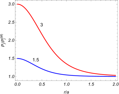
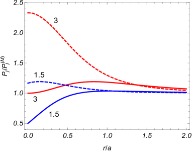
Figure 1: The ratio of the Casimir pressure for a massless scalar field to the corresponding quantity in the Minkowski bulk versus the distance from the string. The left and right panels are for Dirichlet and Neumann boundary conditions respectively. The numbers near the curves are the values of the parameter $q$. On the right panel, the full and dashed curves correspond to minimally and conformally coupled scalars, respectively.

Another special case corresponds to Dirichlet boundary condition on the plate $z=a_{1}$ ($\beta_{1}=0$) and Neumann boundary condition on the second plate $z=a_{2}$ ($\beta_{2}=\infty$). The corresponding expressions for the function $F_{j}(s,r)$ is obtained from (6.3) taking $c_{j}(au)=(-1)^{j}$, $h_{1}(au)=0$ and $h_{2}(au)=4$. We can obtain an equivalent representations by using the expansion for the function $(e^{2au}+1)^{-1}$ which is the analog of (3.25). The expressions for $F_{1}(s,r)$ are obtained from the formulas (6.8) and (6.9) for the function $F_{j}^{(D)}(s,r)$ adding the factor $(-1)^{n}$ in the expression under the sign of the summation. The expressions for $F_{2}(s,r)$ are obtained from (6.10) and (6.12) in a similar way. For even values of $D$ and for a massless field the series over $n$ is summed taking the derivatives of the relation

$$\sum_{n=1}^{\infty}\frac{(-1)^{n}}{\pi^{2}n^{2}+b^{2}}=\frac{b/\sinh b-1}{2b^{2}}.$$ (6.18)

In particular, for $D=4$ we can show that

$$F_{1}^{(DN)}(s,r) = \frac{1}{8\sqrt{2\pi}r^{4}s^{4}}\left(b^{3}\frac{2+\sinh^{2}b}{\sinh^{3}b}-2\right),$$

$$F_{2}^{(DN)}(s,r) = F_{1}^{(DN)}(s,r)+\frac{\xi-1/4}{\sqrt{2\pi}r^{4}s^{2}}\left[\frac{b}{\sinh b}\left(\frac{2b^{2}}{\sinh^{2}b}+b\coth b+b^{2}+1\right)-4\right],$$ (6.19)

with the same $b$ as in (6.16).

For the model with $D=4$, figure 2 displays the ratio $P_{j}/P_{j}^{(M)}$ versus $r/a$ for Dirichlet boundary condition on the plate $z=a_{1}$ and Neumann boundary condition on the plate $z=a_{2}$. The graphs are plotted for a massless field and for two values of the parameter $q$ (numbers near the curves). The left and right panels correspond to the plates $z=a_{1}$ and $z=a_{2}$, respectively. For the right panel, the full/dashed lines correspond to minimally/conformally coupled scalar fields. For the considered example we have $P_{j}^{(M)}=7\pi^{2}a^{-4}/3840$ and the corresponding forces are repulsive.

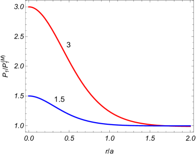
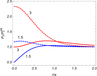
Figure 2: The ratio of the Casimir pressures for a massless scalar field in $D=4$ cosmic string and Minkowski backgrounds in the case of Dirichlet boundary condition at $z=a_{1}$ and Neumann boundary condition at $z=a_{2}$. The left (right) panel presents the pressure on the plate $z=a_{1}$ ($z=a_{2}$). On the right panel, the full and dashed curves correspond to minimally and conformally coupled scalars, respectively. The numbers near the curves are the values of the parameter $q$.

6.2 Shear force

As it has been emphasized above, in the problem at hand in addition to the normal Casimir force one has a nonzero shear force along the radial direction, $dF_{(j)}^{1}=f_{(j)}dS$, where $f_{(j)}$ is the shear force per unit surface of the plate at $z=z_{j}$. The latter is given by $f_{(j)}=\langle T_{3}^{1}\rangle|_{z=a_{j}+0}^{z=a_{j}-0}$ (note that the limiting transitions $r\rightarrow 0$ and $z\rightarrow a_{j}\pm 0$ are not commutative).

Let us start with the case of a single plate at $z=z_{j}$. The corresponding shear forces acting on the sides $z=a_{j}-0$ and $z=a_{j}+0$ coincide and by using (4.19) with the function $U_{3}^{(j)1}(s,r,z)$ from (4.34) for $r\neq 0$ one gets

$$f_{j}^{(1)}=\frac{4\beta_{j}\left(1-4\xi\right)}{(2\pi)^{D/2}r}\left[\sideset{}{{}^{\prime}}{\sum}_{k=1}^{[q/2]}U^{(j)}(rs_{k})-\frac{q}{\pi}\int_{0}^{\infty}dy\frac{\sin(q\pi)U^{(j)}(r\cosh y)}{\cosh(2qy)-\cos(q\pi)}\right],$$ (6.20)

where

$$U^{(j)}(y)=4m^{D+2}y^{2}\int_{0}^{\infty}dx\,xe^{-x}f_{D/2+1}(m\sqrt{\beta_{j}^{2}x^{2}+4y^{2}}).$$ (6.21)

The shear force vanishes for Dirichlet and Neumann boundary conditions. At large distances from the string, $mr\gg 1$, the dominant contribution to (6.20) comes from the $k=1$ term and to the leading order

$$f_{j}^{(1)}\approx\frac{2\beta_{j}\left(1-4\xi\right)}{(2\pi)^{(D-1)/2}r}\frac{m^{D}e^{-2mr\sin(\pi/q)}}{[2mr\sin(\pi/q)]^{(D-1)/2}}.$$ (6.22)

Note that the dependence of the shear force on the curvature coupling parameter $\xi$ appears in the form of the coefficient $1-4\xi$. Near the string, $mr\ll 1$, the shear stress (6.20) behaves as $r^{1-D}$ for $r\ll m^{-1},|\beta_{j}|$, and as $r^{-D-1}$ for $|\beta_{j}|\ll r\ll m^{-1}$. The divergence on the string of the self-shear stress is a consequence of the idealized model of the cosmic string with zero thickness core. In more realistic models, the behavior of the shear stress near the string depends on the core structure.

For a massless field we have

$$U^{(j)}(y)=2^{D/2+2}y^{2}\int_{0}^{\infty}dx\,\frac{\Gamma(D/2+1)xe^{-x}}{(\beta_{j}^{2}x^{2}+4y^{2})^{D/2+1}}.$$ (6.23)

In this case the decay of the shear stress at large distances is as power law:

$$f_{j}^{(1)}\approx\frac{4\beta_{j}\left(1-4\xi\right)}{(4\pi)^{D/2}r^{D+1}}\Gamma(D/2+1)g_{D}(q),$$ (6.24)

with the function $g_{D}(q)$ defined in (4.9). In figure 3 we have plotted the shear stress $f_{j}^{(1)}$ for a $D=4$ massless field as a function of the radial coordinate (left panel, arbitrary units) and of the coefficient in the Robin boundary condition (right panel, arbitrary units). The left panel is plotted for $\beta_{j}=-1$ and the right panel is plotted for $r=0.5$. The numbers near the curves are the corresponding values of the parameter $q$.

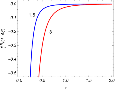
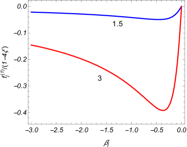
Figure 3: The shear stress on a single plate for a $D=4$ massless scalar field as a function of the radial coordinate and of the Robin coefficient (arbitrary units). The numbers near the curves correspond to the values of $q$.

In the geometry of two plates the shear force per unit surface of the plate at $z=a_{j}$ is presented as

$$f_{j}=f_{j}^{(1)}+f_{jj^{\prime}},$$ (6.25)

where $f_{jj^{\prime}}=\langle T_{3}^{1}\rangle_{jj^{\prime}}|_{z=a_{j}+0}^{z=a_{j}-0}$ is the shear stress induced by the plate at $z=z_{j^{\prime}}$. Note that $f_{jj^{\prime}}=0$ in the regions $z\leqslant z_{1}$ and $z\geqslant z_{2}$ and the force acts on the sides $z=a_{1}+0$ and $z=a_{2}-0$ only. By taking into account (5.28) and (5.30), for the shear stress induced by the second plate one obtains

$$f_{jj^{\prime}}=\frac{4\beta_{j}\left(1-4\xi\right)}{(2\pi)^{D/2}r}\left[\sideset{}{{}^{\prime}}{\sum}_{k=1}^{[q/2]}U^{(jj^{\prime})}(rs_{k})-\frac{q}{\pi}\int_{0}^{\infty}dy\frac{\sin(q\pi)U^{(jj^{\prime})}(r\cosh y)}{\cosh(2qy)-\cos(q\pi)}\right],$$ (6.26)

with the function

$$U^{(jj^{\prime})}(y)=\sqrt{2\pi}y^{2}\int_{m}^{\infty}du\frac{u^{2}(u^{2}-m^{2})^{(D-1)/2}}{c_{1}(au)c_{2}(au)e^{2au}-1}\frac{Z_{(D-1)/2}(2y\sqrt{u^{2}-m^{2}})}{1-\beta_{j}^{2}u^{2}}.$$ (6.27)

Note that, unlike the self-shear, the interaction part (6.26) is finite everywhere, including on the string. Figure 4 presents the interaction part of the shear stress as a function of the ratios $r/a$ (left panel) and $\beta_{j}/a$ (right panel) for a $D=4$ massless scalar field and for $q=1.5,3$ (numbers near the curves) in the model with $\beta_{1}=\beta_{2}$. The left panel is plotted for $\beta_{j}/a=-1$ and the right panel is plotted for $r/a=0.5$.

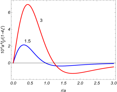
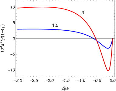
Figure 4: The interaction part of the shear stress in the geometry of two plates for a $D=4$ massless scalar field as a function of $r/a$ and $\beta_{j}/a$. The graphs are plotted for $\beta_{1}=\beta_{2}$.

7 Summary

We have investigated the effects of nontrivial topology due to a straight cosmic string on the local characteristics of the scalar vacuum and on the Casimir forces in the geometry of two parallel plates perpendicular to the axis of the string. On the plates, the Robin boundary conditions are imposed with coefficients that, in general, can differ for separate plates. In the problem under consideration all the properties of the quantum vacuum are encoded in two-point functions. As the first step for the evaluation of these functions we have constructed the heat-kernel as a mode-sum over the complete set of scalar modes. The mode-sum contains summation over the eigenvalues for the component of the momentum perpendicular to the plates. Unlike to special cases of Dirichlet and Neumann boundary conditions, in the region between the plates these eigenvalues are given implicitly, as solutions of the transcendental equation (2.11). For the summation of the corresponding series, we have employed a variant of the generalized Abel-Plana formula that allowed us to extract explicitly the boundary-free contribution in the Green function (see (3.21)) and to present the boundary-induced part, given by (3.22), in terms of integrals strongly convergent for points away from the plates. The boundary-induced contribution to the Green function can be further decomposed into the single boundary and second boundary-induced terms (see (3.17)), separately given by (3.18). For points away from the plates, the local geometry in the problem at hand is Minkwoskian and, as a consequence, the renormalization of the VEVs in the coincidence limit is reduced to the subtraction of the corresponding VEVs in boundary-free Minkowski spacetime. In the representations of the Green function we have provided, the Minkowskian part is presented by the $k=0$ term in the formula (3.18) for the boundary-free function $G_{0}(x,x^{\prime})$. Hence, the renormalized VEVs are obtained omitting this term and taking the coincidence limit of the arguments.

Our consideration of the VEVs of the field squared and of the energy-momentum tensor we have started with the presence of a single plate. The boundary-induced contributions are given by (4.3) and (4.19). The $k=0$ terms in these expressions correspond to the VEVs for a plate in Minkowski bulk. The remaining parts are contributions induced by the nontrivial topology of the cosmic string. In special cases of Dirichlet and Neumann boundary conditions the results for the geometry of a single plate reduce to those previously derived in [17]. For points outside the plates and close to the string, the VEVs are dominated by the boundary-free contributions. The latter diverge on the string as $1/r^{D-2}$ for the field squared and like $1/r^{D}$ for the diagonal components of the energy-momentum tensor. The boundary-induced parts in the VEVs are finite on the string. For the field squared one has a simple relation (4.12) with the corresponding VEV in Minkowski bulk. For the diagonal components of the energy-momentum tensor in the case of a single plate the corresponding relation is more complicated and is given by (4.38). The off-diagonal component linearly vanishes on the string. For points outside from the string the divergences of the VEVs on the boundary coincide with those for a plate in Minkowski bulk and the topological parts are finite on the boundary.

The VEVs in the region between the plates are decomposed into the boundary-free and boundary-induced contributions. The latter is given by (5.2),(5.3) for the VEV of the field squared and and by (5.15),(5.16) for the energy-momentum tensor. The $k=0$ terms in these expressions are the corresponding VEVs in the region between two plates on the Minkowski bulk. For points away from the boundaries, the off-diagonal component of the energy-momentum tensor vanishes on the string. The functions (5.3) and (5.16) in the expressions for the VEVs are further simplified to (5.6) and (5.19) in the special cases of the Dirichlet and Neumann boundary conditions. For the off-diagonal component of the energy-momentum tensor the corresponding function is presented as (5.22). The off-diagonal component vanishes on the plates for Dirichlet and Neumann boundary conditions. Alternative decompositions with the extracted single plate and the second plate-induced parts in the region between the plates are given by (5.10) and (5.27).

In Section 6 we have investigated the Casimir forces acting on the plates. Due to the nonzero off-diagonal component of the vacuum energy-momentum tensor, in addition to the normal component, these forces have nonzero component parallel to the boundary (shear force). The vacuum effective pressure on the plates, corresponding to the normal component of the Casimir force, is given by (6.2) with the function (6.3). The corresponding forces are attractive for $P_{j}<0$ and repulsive for $P_{j}>0$. Unlike the problem on the Minkowski bulk, the forces acting on the separate plates, in general, do not coincide if the corresponding Robin coefficients are different. Another difference is that in the presence of the cosmic string the Casimir forces for Dirichlet and Neumann boundary conditions differ. In these special cases the functions in the expression for the pressures are simplified to (6.7) and (6.10). For a massless field the corresponding formulas take the form (6.9) and (6.12). For odd values of the spatial dimension the corresponding series are expressed in terms of elementary functions (see (6.16) for $D=4$). For Dirichlet boundary condition the Casimir pressure do not depend on the curvature coupling parameter. This is not the case for Neumann boundary condition. A new qualitative feature induced by the cosmic string is the appearance of the shear stress acting on the plates. The corresponding force is directed along the radial coordinate. The shear force vanishes for Dirichlet and Neumann boundary conditions. In the geometry of a single plate, the corresponding stress is given by (6.20) with the function (6.21). At large distances from the string the shear force decays as $e^{-2mr\sin(\pi/q)}$ for a massive field and like $1/r^{D+1}$ for a massless field. In the geometry of two plates the shear stress is decomposed into two contributions (see (6.25)). The first one corresponds to the self-stress and the second one is induced by the presence of the second plate. The latter is given by (6.26) and (6.27). Depending on the parameters of the problem, the radial component of the shear force can be either positive or negative.

The regularization procedure we have used is based on the point-splitting. An alternative regularization procedure, widely discussed in the literature, uses the zeta function for the evaluation of global quantities, like the total vacuum energy, or the local zeta function for the investigation of the local VEVs (for example, the energy density and stresses). In appendix A, on the base of the heat kernel, we have evaluated the off-diagonal and local zeta functions in the problem under consideration.

Appendix A Local zeta function

By using the heat kernel $K(x,x^{\prime};s)$ from (2.25), we can evaluate a more general object, the off-diagonal zeta function (see, for example, [30])

$$\zeta(x,x^{\prime};s)=\frac{\mu^{2s}}{\Gamma\left(s\right)}\int_{0}^{\infty}du\,u^{s-1}K(x,x^{\prime};u),$$ (A.1)

where $\mu$ is a mass parameter introduced by dimensional reasons. By taking into account the expression (2.25) for the heat kernel, one gets

$$\zeta(x,x^{\prime};s)=\frac{\left(2\pi\right)^{\frac{1-D}{2}}\mu^{2s}}{2^{s-2}\Gamma\left(s\right)}\left[\sum_{k}S(w_{k},x,x^{\prime};s)-\frac{q}{2\pi}\sum_{l=\pm 1}\int_{0}^{\infty}dy\frac{\sin(q\pi+lq\Delta\varphi)S(w_{y},x,x^{\prime};s)}{\cosh(qy)-\cos(q\pi+lq\Delta\varphi)}\right],$$ (A.2)

with the function

$$S(w,x,x^{\prime};s)=\frac{1}{2a}\sum_{p=1}^{\infty}\frac{(m^{2}+k_{z}^{2})^{\frac{D-1}{2}-s}f_{\frac{D-1}{2}-s}(\sigma(w)\sqrt{m^{2}+k_{z}^{2}})}{1+\cos[y_{p}+2\tilde{\gamma}_{j}(y_{p})]\sin(y_{p})/y_{p}}g_{j}(z,z^{\prime},k_{z}),$$ (A.3)

and $k_{z}=y_{p}/a$. Note that $G(x,x^{\prime})=\zeta(x,x^{\prime};1)/\mu^{2}$.

Further transformation of the function is similar to that we have used for the function $S(w,x,x^{\prime})$ in (3.2). By using the summation formula (3.6), the following decomposition is obtained

$$S(w,x,x^{\prime};s)=S_{0}(w,x,x^{\prime};s)+S_{j}(w,x,x^{\prime};s)+S_{jj^{\prime}}(w,x,x^{\prime};s),$$ (A.4)

where the expressions for the functions in the right-hand side are obtained from the corresponding expressions in (3.14) by the replacement $(D-3)/2\rightarrow(D-1)/2-s$. As a consequence, the off-diagonal zeta function in the region between the boundaries is presented as

$$\zeta(x,x^{\prime};s)=\zeta_{0}(x,x^{\prime};s)+\zeta_{\mathrm{b}}(x,x^{\prime};s),$$ (A.5)

where $\zeta_{0}(x,x^{\prime};s)$ is the corresponding function for the geometry in the absence of boundaries and the contribution $\zeta_{\mathrm{b}}(x,x^{\prime};s)$ is induced by the boundaries. The expressions for the functions $\zeta_{0}(x,x^{\prime};s)$ and $\zeta_{\mathrm{b}}(x,x^{\prime};s)$ are obtained from (A.2) by the replacements $S(w_{k},x,x^{\prime};s)\rightarrow S_{0}(w_{k},x,x^{\prime};s)$ and $S(w_{k},x,x^{\prime};s)\rightarrow S_{\mathrm{b}}(w_{k},x,x^{\prime};s)$, respectively, with

$$S_{\mathrm{b}}(w,x,x^{\prime};s)=S_{j}(w,x,x^{\prime};s)+S_{jj^{\prime}}(w,x,x^{\prime};s).$$ (A.6)

The integral representation for the latter is obtained from (3.20) by the replacement $(D-3)/2\rightarrow(D-1)/2-s$.

From (A.5) for the local zeta function $\zeta(x;s)=\zeta(x,x;s)$ one gets

$$\zeta(x;s)=\zeta_{0}(x;s)+\zeta_{\mathrm{b}}(x;s),$$ (A.7)

where

$$\zeta_{0}(x;s) = \zeta_{\mathrm{M}}(x;s)+\frac{2^{2-s}\mu^{2s}m^{D-2s}}{\left(2\pi\right)^{D/2}\Gamma\left(s\right)}\left[\sideset{}{{}^{\prime}}{\sum}_{k=1}^{[q/2]}f_{D/2-s}(2mrs_{k})\right.$$ (A.8)

$$\left.-\frac{q}{\pi}\int_{0}^{\infty}dy\frac{\sin(q\pi)f_{D/2-s}(2mr\cosh y)}{\cosh(2qy)-\cos(q\pi)}\right],$$

is the local zeta function in the absence of boundaries and $\zeta_{\mathrm{M}}(x;s)$ is the corresponding function in Minkowski spacetime. The second term in the right-hand side of (A.8) is induced by the nontrivial topology of the cosmic string. In the region between the boundaries the boundary-induced contribution in (A.7) is given by

$$\zeta_{\mathrm{b}}(x;s)=\frac{\left(2\pi\right)^{\frac{1-D}{2}}\mu^{2s}}{2^{s-3}\Gamma\left(s\right)}\left[\sideset{}{{}^{\prime}}{\sum}_{k=0}^{[q/2]}S_{\mathrm{b}}(s_{k},x;s)-\frac{q}{\pi}\int_{0}^{\infty}dy\frac{\sin(q\pi)S_{\mathrm{b}}(\cosh y,x;s)}{\cosh(2qy)-\cos(q\pi)}\right],$$ (A.9)

with the function

$$S_{\mathrm{b}}(y,x;s) = \frac{1}{4}\int_{m}^{\infty}du\frac{(u^{2}-m^{2})^{(D-1)/2-s}}{c_{1}(au)c_{2}(au)e^{2au}-1}Z_{\frac{D-1}{2}-s}(2ry\sqrt{u^{2}-m^{2}})$$ (A.10)

$$\times\left[2+\sum_{j=1,2}e^{2u|z-a_{j}|}c_{j}(au)\right].$$

For points away from the boundaries this contribution is finite at $s=1$ and the renormalization of the local VEVs is reduced to the one in the boundary-free geometry. In particular, for the VEV of the field squared one gets

$$\langle\phi^{2}\rangle=\lim_{s\rightarrow 1}\mu^{-2}\left[\zeta(x;s)-\zeta_{\mathrm{M}}(x;s)\right].$$

With the boundary-free zeta function (A.8), this leads to the result (4.2) for the boundary-free geometry and to the result (5.2) in the region between two plates. For the evaluation of the VEV of the energy-momentum tensor, in addition to the local zeta function $\zeta(x;s)$, one needs the off-diagonal zeta function $\zeta(x,x^{\prime};s)$. The latter is required for the evaluation of the first term in the right-hand side of (4.14). It is presented as $\lim_{s\rightarrow 1}\lim_{x^{\prime}\rightarrow x}\partial_{\mu^{\prime}}\partial_{\nu}\zeta(x,x^{\prime};s)$.

The renormalization procedure for the boundary-free cosmic string geometry within the framework of the zeta function approach and the comparison with the point-splitting scheme have been discussed in [31]. Note that the expression for the local zeta function in the boundary-free cosmic string geometry, $\zeta_{0}(x;s)$, given in the second paper of Ref. [31], presents this function in the form of the series over the product $mr$. The local zeta function in a related geometry of a wedge with reflecting boundaries is considered in [32]. Note that, unlike to the case of the cosmic string geometry, the problem with the wedge is not homogeneous along the azimuthal direction.

References

- [1] A. Vilenkin and E.P.S. Shellard, Cosmic Strings and Other Topological Defects (Cambridge University Press, Cambridge, England, 1994); M.B. Hindmarsh and T.W.B. Kibble, Rep. Prog. Phys. 58, 411 (1995).
- [2] E. Witten, Phys. Lett. B 153, 243 (1985).
- [3] E.J. Copeland, L. Pogosian, and T.Vachaspati, Class. Quantum Gravity 28, 204009 (2011); D.F. Chernoff and S.-H. Henry Tye, Int. J. Mod. Phys. D 24, 1530010 (2015).
- [4] D.R. Nelson, Defects and Geometry in Condensed Matter Physics (Cambridge University Press, Cambridge, England, 2002); G. E. Volovik, The Universe in a Helium Droplet (Clarendon, Oxford, 2003).
- [5] S. Bellucci, E.R. Bezerra de Mello, A. de Padua, and A.A. Saharian, Eur. Phys. J. C 74, 2688 (2014).
- [6] E.R. Bezerra de Mello and A.A. Saharian, J. High Energy Phys. 04 (2009) 046; E.R. Bezerra de Mello and A.A. Saharian, J. High Energy Phys. 08 (2010) 038 ; A. Mohammadi, E.R. Bezerra de Mello, and A.A. Saharian, Class. Quantum Gravity 32, 135002 (2015); A.A. Saharian, V.F. Manukyan, and N.A. Saharyan, Eur. Phys. J. C 77, 478 (2017).
- [7] E.R. Bezerra de Mello and A.A. Saharian, J. Phys. A: Math. Theor. 45, 115402 (2012); E.R. Bezerra de Mello and A.A. Saharian, Class. Quantum. Grav. 30, 175001 (2013).
- [8] A.C. Ottewill and P. Taylor, Phys. Rev. D 82, 104013 (2010); A.C. Ottewill and P. Taylor, Class. Quantum Grav. 28, 015007 (2011).
- [9] E. Elizalde, S.D. Odintsov, A. Romeo, A.A. Bytsenko, and S. Zerbini, Zeta Regularization Techniques with Applications (World Scientific, Singapore, 1994); V.M. Mostepanenko and N. N. Trunov, The Casimir Effect and Its Applications (Clarendon, Oxford, 1997); K. A. Milton, The Casimir Effect: Physical Manifestation of Zero-Point Energy (World Scientific, Singapore, 2002); V.A. Parsegian, Van der Waals Forces: A Handbook for Biologists, Chemists, Engineers, and Physicists (Cambridge University Press, Cambridge, England, 2005); M. Bordag, G.L. Klimchitskaya, U. Mohideen, and V.M. Mostepanenko, Advances in the Casimir Effect (Oxford University Press, New York, 2009); Casimir Physics, edited by D. Dalvit, P. Milonni, D. Roberts, and F. da Rosa, Lecture Notes in Physics Vol. 834 (Springer-Verlag, Berlin, 2011).
- [10] E.R. Bezerra de Mello, V.B. Bezerra, A.A. Saharian, and A.S. Tarloyan, Phys. Rev. D 74, 025017 (2006).
- [11] V.V. Nesterenko and I.G. Pirozhenko, Class. Quantum Grav. 28, 175020 (2011).
- [12] E.R. Bezerra de Mello, V.B. Bezerra, A.A. Saharian, and A.S. Tarloyan, Phys. Rev. D 78, 105007 (2008).
- [13] E.R. Bezerra de Mello, V.B. Bezerra, A.A. Saharian, and V.M. Bardeghyan, Phys. Rev. D 82, 085033 (2010); S. Bellucci, E.R. Bezerra de Mello, and A.A. Saharian, Phys. Rev. D. 83, 085017 (2011); E.R. Bezerra de Mello, F. Moraes, and A.A. Saharian, Phys. Rev. D 85, 045016 (2012).
- [14] I. Brevik and T. Toverud, Class. Quantum Grav. 12, 1229 (1995).
- [15] E.R. Bezerra de Mello, V.B. Bezerra, and A.A. Saharian, Phys. Lett. B 645, 245 (2007).
- [16] G. Fucci and K. Kirsten, J. High Energy Phys. 03 (2011) 016; G. Fucci and K. Kirsten, J. Phys. A: Math. Theor. 44, 295403 (2011).
- [17] E.R. Bezerra de Mello and A.A. Saharian, Class. Quantum Grav. 28, 145008 (2011).
- [18] E.R. Bezerra de Mello, A.A. Saharian, and A.Kh. Grigoryan, J. Phys. A: Math. Theor. 45, 374011 (2012).
- [19] E.R. Bezerra de Mello, A.A. Saharian, and S.V. Abajyan, Class. Quantum Grav. 30, 015002 (2013).
- [20] A.Kh. Grigoryan, A.R. Mkrtchyan, and A.A. Saharian, Int. J. Mod. Phys. D 26, 1750064 (2017).
- [21] E.R. Bezerra de Mello and A.A. Saharian, Class. Quantum Grav. 29, 035006 (2012); E.R. Bezerra de Mello and A.A. Saharian, Eur. Phys. J. C 73, 2532 (2013); S. Bellucci, E.R. Bezerra de Mello, A. de Padua, and A.A. Saharian, Eur. Phys. J. C 74, 2688 (2014).
- [22] A. Romeo and A.A. Saharian, J. Phys. A: Math. Gen. 35, 1297 (2002).
- [23] A.A. Saharian, Nucl. Phys. B 712, 196 (2005); E. Elizalde, A.A. Saharian, and T.A. Vardanyan, Phys. Rev. D 81, 124003 (2010); E.R. Bezerra de Mello, A.A. Saharian, and M.R. Setare, Phys. Rev. D 95, 065024 (2017).
- [24] I.S. Gradshteyn and I.M. Ryzhik, Table of Integrals, Series and Products (Academic Press, New York, 1980).
- [25] A.P. Prudnikov, Yu.A. Brychkov, and O.I. Marichev, Integrals and Series (Gordon and Breach, New York, 1986), Vol. 2.
- [26] M. Abramowitz and I. A. Stegun, Handbook of Mathematical Functions (Dover, New York, 1972).
- [27] E. R. Bezerra de Mello and A. A. Saharian, Class. Quantum Grav. 29, 035006 (2012).
- [28] J. Spinelly and E.R. Bezerra de Mello, J. High Energy Phys. 12 (2008) 081.
- [29] A. A. Saharian, The Generalized Abel-Plana Formula with Applications to Bessel Functions and Casimir Effect (Yerevan State University Publishing House, Yerevan, 2008); Preprint ICTP/2007/082; arXiv:0708.1187.
- [30] V. Moretti, Phys. Rev. D 56, 7797 (1997); V. Moretti, Commun. Math. Phys. 201, 327 (1999); A.A. Bytsenko, G. Cognola, E. Elizalde, V. Moretti, and S. Zerbini, Analytic Aspects of Quantum Fields (World Scientific, Singapore, 2003).
- [31] S. Zerbini, G. Cognola, and L. Vanzo, Phys. Rev. D 54, 2699 (1996); D. Iellici, Class. Quantum Grav. 11, 3287 (1997); D. Iellici and V. Moretti, Phys. Lett. B 425, 33 (1998); V. Moretti, J. Math. Phys. 40, 3843 (1999).
- [32] V.N. Nesterenko, G. Lambiase, and G. Scarpetta, Ann. Phys. 298, 403 (2002).