Black Hole Metric: Overcoming the PageRank Normalization Problem

Abstract

In network science, there is often the need to sort the graph nodes. While the sorting strategy may be different, in general sorting is performed by exploiting the network structure. In particular, the metric PageRank has been used in the past decade in different ways to produce a ranking based on how many neighbors point to a specific node. PageRank is simple, easy to compute and effective in many applications, however it comes with a price: as PageRank is an application of the random walker, the arc weights need to be normalized. This normalization, while necessary, introduces a series of unwanted side-effects. In this paper, we propose a generalization of PageRank named Black Hole Metric which mitigates the problem. We devise a scenario in which the side-effects are particularily impactful on the ranking, test the new metric in both real and synthetic networks, and show the results.

1 Introduction

In the vast amount of digital data, humans have the need to discriminate those relevant for their purposes to effectively transform them into useful information, which usefulness depends on the scenario being considered. For instance, in web searching we aim at finding significant pages with respect to an issued query [36], in an E-learning context we look for useful resources within a given topic [9, 40, 41], or in a recommendation network we search for most reliable entities to interact with [15, 14, 21, 4]. All these situations fall under the umbrella of ranking, a challenge addressed in these years through different solutions. The most well-known technique is probably the PageRank algorithm [8, 32], originally designed to be the core of the Google (www.google.com) web search engine. Since it was published it has been analyzed [34, 6, 24], modified or extended for use in other contexts [46, 19], to overcome some of its limitations, and to address computational issues [25, 35].

PageRank has been widely adopted in several different application scenarios. In this paper, we propose a generalization of PageRank whose motivation stems from the concept of trust in virtual social networks. In this context trust is generally intended as a measure of the assured reliance on a specific feature of someone [28, 16, 1], and it is exploited to rank participants in order to discover the best entities that is ”safe” to interact with. This trust-based ranking approach allows to cope with uncertainty and risks [37], a feature especially relevant in the case of lack of bodily presence of counterparts.

A notable limitation of PageRank when it’s used to model social behaviour, is its inability to preserve the absolute arc weights due to the normalization introduced by the application of the random walker. In order to illustrate the problem, we introduce a weighted network where arcs model relationships among entities. Entities may be persons, online shops, computers that in general need to establish relationships with other entities of the same type. Let’s suppose to have the network shown in Figure 1(a), where each arc weight ranges over $[0,10]$.

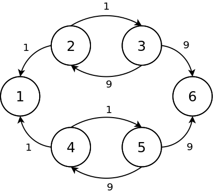
(a) Before the normalization

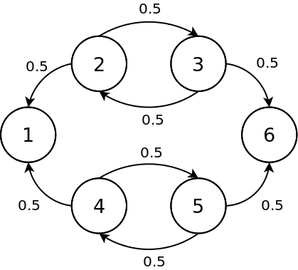
(b) After the normalization

Figure 1: Network with asymmetric trust distribution

Given the network topology, intuition suggests that node 1 would be regarded more poorly compared to node 6 since it receives lower trust values from his neighbors, but, as detailed later, normalizing the weights alters the network topology so much that both nodes are placed in the same position in the ranking. The normalization of the outlink weights indeed hides the weight distribution asymmetry, as depicted in Figure 1(b).

Moreover, PageRank shadows the social implications of assigning low weights to all of a node’s neighbours. If we consider the arcs as if they were social links, common sense would tell us to avoid links with low weight, as they usually model worse relationships. If we look at the normalized weights in Figure 1(b) though, we can see that in many cases, the normalized weight changes the relationship in a counter-intuitive way. Consider the arcs going from node 2 or 4 to their neighbours: we can see that their normalized weights are set to 0.5, which, in the range $[0,1]$ is an average score. However, the original weight of those links was 1, a comparatively lower score considering that the original range was $[0,10]$.

The contribution of this paper is the proposal of a new PageRank-based metric we name Black Hole Metric to cope with the normalization effect and to deal with the issue of the skewed arc weights, detalied in Section 4. Note that our proposal seamlessly adapts to any situation where PageRank can be used, being not limited to trust networks; in the following, they are considered as a simple case study.

The paper is organized as follows: in section  2 we give an overview of the existing literature concerning PageRank, in section 3 we describe the PageRank algorithm together with some of its extensions, whereas in section 4 we illustrate our proposal in detail, comparing it to the basic PageRank in section 5, where we also show some first experiments. Finally, in section 6 we provide our conclusions and some open discussions.

2 Related Works

PageRank is essentially an application of the random walker model on a Markov chain: the nodes of the Markov chain are the web pages, and the arcs are the links that connect one page to another. The walker represents a generic web surfer which moves from page to page with a certain probability, according to the network structure, and occasionally ”gets bored” and jumps to a random node in the network. The steady-state probability vector of the random walker process holds the PageRank values for each node, which can be used to determine the global ranking.

Before describing in detail the normalization problem by showing the issues that may occur, we briefly introduce the web ranking metric that would lay the foundation to modern search engines. As previously mentioned, the PageRank algorithm has been thoroughly analysed, both in its merits and in its shortcomings. Although Pagerank was proposed a long time ago, it still lives as the backbone of several technologies, not limited to the web domain. For example, in [19], personalized PageRank is cited as a possible algorithm to be used in Twitter’s ”Who To Follow” architecture. In [18], the author shows how the mathematics behind PageRank have been used in a plethora of applications which are not limited to ranking pages on the web. In [39], another PageRank extension appears as a tentative replacement of the h-index for publications. A recent technology that uses personalized PageRank as its backend is SwiftType (https://swiftype.com/) which is gaining popularity as a search engine for various platforms.

These examples, however, do not use the basic version of PageRank, but some sort of extension that better fits the domain in which it is applied. To the best of our knowledge, the original PageRank algorithm is seldom used ”as it is”, our proposal itself is an alternative to the weighted PageRank algorithm described in [44]. Besides our work, there are several other extensions that were proposed in the past. For example, CheiRank [46] focuses on evaluating the outlink strength instead of the inlink strength, with the ultimate effect of rewarding hub behaviour, making it essentially a dual metric of PageRank. DirichletRank [43] is a derivative metric which claims to solve the ”zero-one gap problem” of the original PageRank (in brief, the teleportation chance drops from $1$ to $d$, where $d<1$, when the number of outlinks change from 0 to 1). [35] proposes a query-based PageRank in which the random walker probabilities are dependent on the query relevance.

These variants are essentially alternatives or improvements, but several other works either focus on providing shorter runtime, or are adaptations of PageRank to different domains. For instance, [3] proposes a Monte Carlo technique to perform fast computation of random walk based algorithms such as PageRank. There also exists at least a version of distributed PageRank [48] which better handles the ever increasing number of web pages to rank: one of the main shortcoming of basic PageRank is the inability of holding large link matrices entirely in main memory, resulting in slowed down I/O operation; the distributed version of the algorithm takes care of this problem. Another approach [2] handles large data samples by making use of the MapReduce algorithm, introducing PageRank to the world of Big Data. Other types of optimization methods can be found in the surveys [5] and [38]. An important extension of PageRank that operates on the trust network domain[12][11][13], is EigenTrust [20]. Since the application scenario involves trust networks, the entities involved change slightly: web pages are replaced with network nodes, links are replaced with arcs. The underlying mathematics, however, remain essentially unchanged.

PageRank and its extensions have to face a plethora of competitors in several application domains. In the web domain we have HITS [22], which is not based on the random walker model and is able to provide both an ”authority” ranking, which rewards nodes that have many backlinks, and a ”hub” ranking, which rewards nodes that have many forward links. SALSA [27] computes a random walk on the network graph, but integrates the search query into the algorithm, which is something PageRank does not do. In the trust networks domain we have PeerTrust [45], which computes the global trust by aggregating several factors, and PowerTrust [47] which uses the concept of ”power nodes”, which are dynamically selected, high reliability nodes, that serve as moderators for the global reputation update process. The PowerTrust article also describes how the algorithm compares to EigenTrust with a set of simulations that analyse its performance. Several articles feature side-by-side comparisons among PageRank (and its extensions) and other metrics [42, 33, 30]. In particular, [26] focuses on comparing HITS, PageRank and SALSA, and its authors prove that PageRank is the only metric that guarantees algorithmic stability with every graph topology.

3 PageRank

3.1 Definitions and Notation

In order to better understand the mathematics of the Black Hole Metric, we need to clarify the notation used throughout this paper and provide a few definitions, which are similar to the notations used in the article of PageRank. Let us suppose that $N$ is the number of nodes in the network. We will call $A$ the $N\times N$ network adjacency matrix or link matrix, where each $a_{ij}$ is the weight of the arc going from node $i$ to node $j$. $S$ is the $N\times 1$ sink vector, defined as:

$$s_{i}=\begin{cases}1&\mbox{if }{out}_{i}=0\\ 0&\mbox{otherwise}\end{cases}\quad\forall i\leq N$$

where ${out}_{i}$ is the number of outlinks of node $i$. $V$ is the personalization vector of size $1\times N$, equal to the transposed initial distribution probability vector in the Markov chain model $P_{0}^{\mathsf{T}}$. While this vector can be arbitrarily chosen as long as it’s stochastic, a common choice is to make each term equal to $\nicefrac{{1}}{{N}}$. $T=\boldsymbol{1}_{N\times 1}$ is the teleportation vector, where the notation $\boldsymbol{1}_{N\times M}$ stands for a $N\times M$ matrix where each element is $1$.

In the general case the Markov chain built upon the network graph is not always ergodic, so it is not used directly for the calculation of the steady state random walker probabilities. As described in [32], the transition matrix $M$, used in the associated random walker problem, is derived from the link matrix, the sinks vector, the teleportation vector and the personalization vector defined above:

$$M=d(A+SV)+\left(1-d\right)TV$$ (1)

where $d\in[0,1]$ is called damping factor and it is commonly set to $0.85$. As we know from the Markov chain theory, the random walk probability vector at step $n$ can be calculated as:

$$P_{n}=M^{\mathsf{T}}P_{n-1}$$ (2)

the related random walker problem can be calculated as:

$$P=\left(\lim_{n\to\infty}M^{n}\right)^{\mathsf{T}}P_{0}=\lim_{n\to\infty}(M^{\mathsf{T}})^{n}P_{0}=M_{\infty}^{\mathsf{T}}P_{0}$$ (3)

3.2 The normalization problem

Let us calculate the PageRank values of the sample network in Figure 1(a) to highlight the flattening effect of the normalization. By applying the definitions in section 3.1 the network in Figure 1(b) can be described by the following matrices and vectors:

$$A=\begin{pmatrix}0&0&0&0&0&0\\[3.00003pt] 0.5&0&0.5&0&0&0\\[3.00003pt] 0&0.5&0&0&0&0.5\\[3.00003pt] 0.5&0&0&0&0.5&0\\[3.00003pt] 0&0&0&0.5&0&0.5\\[3.00003pt] 0&0&0&0&0&0\end{pmatrix}\quad S=\begin{pmatrix}1\\[3.00003pt] 0\\[3.00003pt] 0\\[3.00003pt] 0\\[3.00003pt] 0\\[3.00003pt] 1\end{pmatrix}\quad V=P_{0}^{\mathsf{T}}=\frac{1}{6}\cdot\boldsymbol{1}_{1\times 6}\quad T=\boldsymbol{1}_{6\times 1}$$

If we calculate the PageRank values for the nodes of the sample network assuming $d=0.85$ we obtain:

$$p_{1}=p_{6}=0.208\quad p_{2}=p_{3}=p_{4}=p_{5}=0.146$$

Note that the nodes 1 and 6 are both first in global ranking, despite the fact that their in-strength was so different before the normalization.

4 Black Hole Metric

In order to avoid the flattening effect of the PageRank normalization, we propose a new metric named Black Hole Metric. Black Hole Metric globally preserves the proportions among the arc weights, and ensures at the same time that the outstrength is equal to 1 for each node. This allows compatibility with the random walker model, and it is done by applying a transformation to the original network. The transformation only requires the knowledge of the maximum and the minimum value each weight can assume. This range bounds may be global (each node has the same scale) or local (each node has its own weight scale); in practice, global scale is preferred.

At this stage, we will provide an example of the transformation steps as illustrated in Figure 2. In order to obtain the depicted values, we used formulas (4) and (7), which will be explained in detail in paragraph 4.1. Before tackling the mathematical part though, we will now describe qualitatively how the Black Hole Metric operates. First, it changes the original weights so that they lie in the range $[0,1]$. The resulting outstrength $s_{i}$ of each node $i$ is not preserved, but it is guaranteed to be less or equal than 1. Then, we introduce a new node, the black hole, and node $i$ is connected to it. The strength of this connection is set to $1-s_{i}$, as if the black hole ”absorbed” the missing weight amount to reach 1 as the total $i$’s outstrenght. This transformation is applied to all nodes in the network.

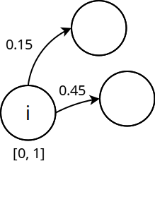
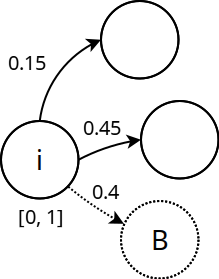
Figure 2: Transformation steps

Since the black hole does not have outlinks, it is a sink by construction, and the random walker can only move away because of the teleportation effect. In a network without the black hole, each node would normally have a $1-d$ chance to teleport to a random node instead of going towards one of its neighbours. We know that moving to the black hole from node $i$ occurs with a $1-s_{i}$ chance, and that once in the black hole, the random walker inevitably teleports to a random node. In conclusion, taking both effects into account, each node has a $(1-d)(1-s_{i})$ chance to teleport to a random node, where $d$ is the damping factor as in (1).

It is important to note that not every network has a defined scale for its arc weights. There are networks in which the weights are unbounded: an example would be an airline transportation network in which each arc weight is the number of flights connecting two cities. As there is no real ”maximum”, there is no trivial weight scale that can be used for the transformation. In order to apply such transformation in an unbounded network, we need to somehow infer meaningful scale boundaries exploiting the knowledge of the domain, and the topology of the network. This is usually non-trivial and for the sake of simplicity, in this paper we take into account only bounded networks.

4.1 Weight assignment

In this section, we explain how the new weights are calculated. Let $i$ be a generic node in the network. Let the interval $[l_{i},h_{i}]$ be the local scale of node $i$. Let $r_{ij}$ be the weight that node $i$ assigns to the arc pointing towards node $j$. Let ${out}_{i}$ be the number of neighbours of node $i$. Given that $l_{i}\leq r_{ij}\leq h_{i}$, We define the modified weight $\bar{a}_{ij}$ of the arc that goes from $i$ to $j$ as:

$$\bar{a}_{ij}=\frac{r_{ij}-l_{i}}{{out}_{i}(h_{i}-l_{i})}$$ (4)

which is significantly different from the normalized arc weight required by PageRank:

$$a_{ij}=\frac{r_{ij}}{\sum_{k=1}^{{out}_{i}}r_{ik}}$$ (5)

As mentioned before, the resulting node outstrength is only guaranteed to be less or equal to 1:

$$\sum_{j=1}^{{out}_{i}}\bar{a}_{ij}=\sum_{j=1}^{{out}_{i}}\frac{r_{ij}-l_{i}}{{out}_{i}(h_{i}-l_{i})}\leq\sum_{j=1}^{{out}_{i}}\frac{1}{{out}_{i}}=1$$ (6)

We purposely excluded the contribute of the arc from node $i$ to the black hole in (6), which is:

$$b_{i}=\sum_{j=1}^{{out}_{i}}\frac{h_{i}-r_{ij}}{{out}_{i}(h_{i}-l_{i})}$$ (7)

If we include this contribute as well, the weight sum becomes 1 as desired:

$$\sum_{j=1}^{{out}_{i}}\bar{a}_{ij}+b_{i}=\sum_{j=1}^{{out}_{i}}\frac{r_{ij}-l_{i}}{{out}_{i}(h_{i}-l_{i})}+\sum_{j=1}^{{out}_{i}}\frac{h_{i}-r_{ij}}{{out}_{i}(h_{i}-l_{i})}=\sum_{j=1}^{{out}_{i}}\frac{h_{i}-l_{i}}{{out}_{i}(h_{i}-l_{i})}=1$$ (8)

The weight $b_{i}$ is ultimately the probability that the node would rather visit a random node rather than one of its neighbours, which is the amplification of the teleportation effect operated by the network transformation described before.

4.2 Proposal

With the previously mentioned weight assignment, it is now possible to define Black Hole Metric as a generalization of PageRank. Let’s start by defining the new link matrix $A^{\prime}$, the new sink vector $S^{\prime}$, the new teleportation vector $T^{\prime}$ and the new personalization vector $V^{\prime}$.

For the sake of convenience, we name $B$ the black hole vector, which is the $N\times 1$ vector that holds the weights of the arcs going from each node to the black hole. The updated link matrix $A^{\prime}$ is obtained by combining the $B$ vector with $\bar{A}=\{\bar{a}_{ij}\}$ where $\bar{a}_{ij}$ is defined in (4):

$$A^{\prime}=\begin{pmatrix}\bar{A}&B\\[3.00003pt] \boldsymbol{0}_{1\times N}&0\end{pmatrix}$$ (9)

In general, $A\neq\bar{A}$. There are other three entities involved in the computation of the transition matrix used by the random walker model: the teleportation vector $T^{\prime}$, the personalization vector $V^{\prime}$, and the sink vector $S^{\prime}$. We may define $T^{\prime}$ and $V^{\prime}$ as follows:

$$V^{\prime}={P^{\prime}_{0}}{}^{\mathsf{T}}=\begin{pmatrix}V&0\end{pmatrix}=\begin{pmatrix}\frac{1}{N}\cdot\boldsymbol{1}_{1\times N}&0\end{pmatrix}\quad T^{\prime}=\begin{pmatrix}T\\[3.00003pt] 0\end{pmatrix}=\begin{pmatrix}\boldsymbol{1}_{N\times 1}\\[3.00003pt] 0\end{pmatrix}$$ (10)

Note that we deliberately excluded the black hole from the teleportation effect by putting a value of $0$ in the corresponding entries of $T^{\prime}$ and $V^{\prime}$. Since the black hole is a sink by construction, going back there as the consequence of a teleportation effect would only trigger another teleportation effect, which is unnecessary.

Regarding the sink vector, we intuitively want to set to $1$ the corresponding index in the vector, as the black hole is a sink, but this actually makes the black hole row in the link matrix not stochastic. Let’s consider the matrix $A^{\prime}$ defined above, and let’s use the following sink vector to compute the transition matrix:

$$S^{*}=\begin{pmatrix}S\\[3.00003pt] 1\end{pmatrix}$$ (11)

We can calculate $M^{\prime}$ using (1):

$$\begin{split}M^{\prime}=d(A^{\prime}+S^{*})+(1-d)T^{\prime}V^{\prime}=d\left[\begin{pmatrix}\bar{A}&B\\[3.00003pt] \boldsymbol{0}_{1\times N}&0\end{pmatrix}+\begin{pmatrix}SV&\boldsymbol{0}_{N\times 1}\\[3.00003pt] V&0\end{pmatrix}\right]+\\ +(1-d)\begin{pmatrix}TV&\boldsymbol{0}_{N\times 1}\\[3.00003pt] \boldsymbol{0}_{1\times N}&0\end{pmatrix}=\begin{pmatrix}d(\bar{A}+SV)+(1-d)TV&dB\\[3.00003pt] dV&0\end{pmatrix}\end{split}$$

The black hole row in the link matrix is $dV$, which is not stochastic: the vector $V$ is, but since $d\neq 1$ the product is not. This happened because we excluded the black hole from the teleportation effect by setting its entry to $0$ in $T^{\prime}$, which interferes with the damping factor correction. In order to compensate for this effect, it is sufficient to multiply the black hole entry in the sink vector by a $\frac{1}{d}$ term:

$$S^{\prime}=\begin{pmatrix}S\\[3.00003pt] \frac{1}{d}\end{pmatrix}$$ (12)

this makes the black hole row in the link matrix $V$, which is stochastic. Equations (9), (10) and (12) allow us to define the random walker model according to the definition of $M$ in (1):

$$M^{\prime}=d(A^{\prime}+S^{\prime}V^{\prime})+\left(1-d\right)T^{\prime}V^{\prime}$$

We can now partition $M^{\prime}$:

$$\begin{split}M^{\prime}=d\begin{pmatrix}\bar{A}&B\\[3.00003pt] \boldsymbol{0}_{1\times N}&0\end{pmatrix}+d\begin{pmatrix}S\\[3.00003pt] \frac{1}{d}\end{pmatrix}\begin{pmatrix}V&0\end{pmatrix}+(1-d)\begin{pmatrix}T\\[3.00003pt] 0\end{pmatrix}\begin{pmatrix}V&0\end{pmatrix}=\begin{pmatrix}d\bar{A}&dB\\[3.00003pt] \boldsymbol{0}_{1\times N}&0\end{pmatrix}+\\ +\begin{pmatrix}dSV&\boldsymbol{0}_{N\times 1}\\[3.00003pt] V&0\end{pmatrix}+\begin{pmatrix}(1-d)TV&\boldsymbol{0}_{N\times 1}\\[3.00003pt] \boldsymbol{0}_{1\times N}&0\end{pmatrix}=\begin{pmatrix}d\left(\bar{A}+SV\right)+(1-d)TV&dB\\[3.00003pt] V&0\end{pmatrix}\end{split}$$

If we name $\bar{M}=d\left(\bar{A}+SV\right)+(1-d)TV$ we have:

$$M^{\prime}=\begin{pmatrix}\bar{M}&dB\\[3.00003pt] V&0\end{pmatrix}$$ (13)

Consider now the following partition of the rank vector $P^{\prime}$:

$$P^{\prime}=\begin{pmatrix}\bar{P}\\[3.00003pt] p_{b}\end{pmatrix}$$ (14)

where $p_{b}$ is the steady-state probability of the black hole. Note that usually $\bar{P}\neq P$. The rank vector at step $n$, which we named $P^{\prime}_{n}$, can be obtained using (2), (13) and (14):

$$\begin{split}P^{\prime}_{n}=M^{\prime}{}^{\mathsf{T}}P^{\prime}_{n-1}\Leftrightarrow\begin{pmatrix}\bar{P}_{n}\\[3.00003pt] p_{b_{n}}\end{pmatrix}=\begin{pmatrix}\bar{M}^{\mathsf{T}}&V^{\mathsf{T}}\\[3.00003pt] dB^{\mathsf{T}}&0\end{pmatrix}\begin{pmatrix}\bar{P}_{n-1}\\[3.00003pt] p_{b_{n-1}}\end{pmatrix}\Leftrightarrow\begin{pmatrix}\bar{P}_{n}\\[3.00003pt] p_{b_{n}}\end{pmatrix}=\begin{pmatrix}\bar{M}^{\mathsf{T}}\bar{P}_{n-1}+p_{b_{n-1}}V^{\mathsf{T}}\\[3.00003pt] dB^{\mathsf{T}}\bar{P}_{n-1}\end{pmatrix}\end{split}$$

We split the calculation in two parts:

$$\begin{cases}\bar{P}_{n}=\bar{M}^{\mathsf{T}}\bar{P}_{n-1}+p_{b_{n-1}}V^{\mathsf{T}}\\ p_{b_{n}}=dB^{\mathsf{T}}\bar{P}_{n-1}\end{cases}$$ (15)

The related random walker process (3), given the definition of matrix $M^{\prime}$ (13), the definition of the personalization vector $P^{\prime}_{0}=V^{\prime}{}^{\mathsf{T}}$, and the definition of the rank vector of the Black Hole Metric $P^{\prime}$ (14), can be written as:

$$P^{\prime}=M^{\prime}_{\infty}{}^{\mathsf{T}}P^{\prime}_{0}\Leftrightarrow\begin{pmatrix}\bar{P}\\[3.00003pt] p_{b}\end{pmatrix}=\begin{pmatrix}\bar{M}^{\mathsf{T}}&V^{\mathsf{T}}\\[3.00003pt] dB^{\mathsf{T}}&0\end{pmatrix}_{\infty}\begin{pmatrix}P_{0}\\[3.00003pt] 0\end{pmatrix}$$ (16)

An important property of the transition matrix $M^{\prime}$ is that it leads to a converging random walker process no matter the network topology, as it will be clarified in section 4.5. As a final note, even though in general $A\neq\bar{A}$ and $P\neq\bar{P}$, in section 4.6 we will introduce a sufficient condition that allows the identity.

4.3 Application to example toy network

Now that we have defined the necessary entities and described how we assign weights in the modified network, let’s see how Black Hole Metric behaves in the sample trust network in Figure 1(a). For this particular network we set that $l_{i}=l=0,\enspace h_{i}=h=10\enspace\forall i\in[1,N]$. It is easy to note that we have only three types of nodes in the network:

1. Nodes which have two links with weight 1 out of 10 (nodes 2 and 4).

2. Nodes which have two links with weight 9 out of 10 (nodes 3 and 5).

3. Sinks (nodes 1 and 6).

We only show the arc weights of node 2, as the same formulas can be used to calculate the outlink weights of the other nodes. Given that ${out}_{2}=2$ we have:

$$\bar{a}_{21}=\bar{a}_{23}=\frac{r_{21}-l}{{out}_{2}\cdot(h-l)}=\frac{1-0}{2\cdot(10-0)}=\frac{1}{20}$$

The black hole arc weight is going to be:

$$b_{2}=\frac{h-r_{21}+h-r_{23}}{{out}_{2}(h-l)}=\frac{20-2}{2\cdot(10-0)}=\frac{9}{10}$$

as expected, $\bar{a}_{21}+\bar{a}_{22}+b_{2}=1$. By applying the formulas to all arcs we create the network in Figure 3.

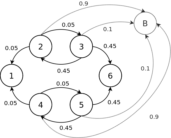
Figure 3: The Network in Figure 1 with the black hole.

The link matrix $A^{\prime}$ as in (9) is:

$$A^{\prime}=\begin{pmatrix}0&0&0&0&0&0&0\\[3.00003pt] 0.05&0&0.05&0&0&0&0.9\\[3.00003pt] 0&0.45&0&0&0&0.45&0.1\\[3.00003pt] 0.05&0&0&0&0.05&0&0.9\\[3.00003pt] 0&0&0&0.45&0&0.45&0.1\\[3.00003pt] 0&0&0&0&0&0&0\\[3.00003pt] 0&0&0&0&0&0&0\end{pmatrix}$$

while $B$ is:

$$B=\begin{pmatrix}0\\[3.00003pt] 0.9\\[3.00003pt] 0.1\\[3.00003pt] 0.9\\[3.00003pt] 0.1\\[3.00003pt] 0\\[3.00003pt] \end{pmatrix}$$

Vectors $S^{\prime}$, $V^{\prime}$ and $T^{\prime}$ are obvious from (10) and (12):

$$S^{\prime}=\begin{pmatrix}1\\[3.00003pt] 0\\[3.00003pt] 0\\[3.00003pt] 0\\[3.00003pt] 0\\[3.00003pt] 1\\[3.00003pt] \frac{1}{d}\end{pmatrix}\quad V^{\prime}={P^{\prime}_{0}}{}^{\mathsf{T}}=\begin{pmatrix}\frac{1}{6}\cdot\boldsymbol{1}_{1\times 6}&0\end{pmatrix}\quad T^{\prime}=\begin{pmatrix}\boldsymbol{1}_{6\times 1}\\[3.00003pt] 0\end{pmatrix}$$

If we compute the steady-state probabilities for the random walker process in (16) assuming $d=0.85$, the values calculated for each node (including the black hole) of the network in Figure 3 are:

$$p_{1}=0.110\quad p_{2}=p_{4}=0.138\quad p_{3}=p_{5}=0.104\quad p_{6}=0.178\quad p_{b}=0.228$$

which better models the trust relationships among the nodes, as $p_{1}<p_{6}$. There is also a value $p_{b}$ for the black hole, which is a consequence of the transformation we operated. Since the black hole is not a real node, this probability does not bear any particular meaning, and it can be discarded.

4.4 Complexity assessment

Using (15) for direct computation, no matter the method in use, is inefficient in both time and space complexity, therefore we will now introduce a more efficient way to solve the problem. First, let us rewrite $\bar{P}_{n}$ appropriately:

$$\bar{P}_{n}=\bar{M}^{\mathsf{T}}\bar{P}_{n-1}+p_{b_{n-1}}V^{\mathsf{T}}=d\bar{A}^{\mathsf{T}}\bar{P}_{n-1}+dV^{\mathsf{T}}S^{\mathsf{T}}\bar{P}_{n-1}+\left(1-d\right)V^{\mathsf{T}}T^{\mathsf{T}}\bar{P}_{n-1}+p_{b_{n-1}}V^{\mathsf{T}}$$

The quantities $T^{\mathsf{T}}\bar{P}_{n-1}=\bar{t}_{p_{n-1}}$ and $S^{\mathsf{T}}\bar{P}_{n-1}=\bar{s}_{p_{n-1}}$ are both scalars. In particular, we have:

$$T^{\mathsf{T}}\bar{P}_{n-1}=\sum_{k=0}^{N}{\bar{p}_{k_{n-1}}}=1-p_{b_{n-1}}$$ (17)

which allows us to write:

$$\begin{split}\bar{P}_{n}=d\bar{A}^{\mathsf{T}}\bar{P}_{n-1}+d\bar{s}_{p_{n-1}}V^{\mathsf{T}}+\left(1-d\right)\bar{t}_{p_{n-1}}V^{\mathsf{T}}+p_{b_{n-1}}V^{\mathsf{T}}=\\ =d\bar{A}^{\mathsf{T}}\bar{P}_{n-1}+[d\bar{s}_{p_{n-1}}+\left(1-d\right)\bar{t}_{p_{n-1}}+p_{b_{n-1}}]V^{\mathsf{T}}\end{split}$$

The quantity under square brackets can be further simplified using (17):

$$d\bar{s}_{p_{n-1}}+\left(1-d\right)\bar{t}_{p_{n-1}}+p_{b_{n-1}}=d\bar{s}_{p_{n-1}}+(1-d)(1-p_{b_{n-1}})+p_{b_{n-1}}=$$

$$=d\bar{s}_{p_{n-1}}+1-d-\cancel{p_{b_{n-1}}}+dp_{b_{n-1}}+\cancel{p_{b_{n-1}}}=1-d(1-\bar{s}_{p_{n-1}}-p_{b_{n-1}})$$

which allows us to write (15) as:

$$\begin{cases}\bar{P}_{n}=d\bar{A}^{\mathsf{T}}\bar{P}_{n-1}+[1-d(1-\bar{s}_{p_{n-1}}-p_{b_{n-1}})]V^{\mathsf{T}}\\ p_{b_{n}}=d\bar{b}_{p_{n-1}}\end{cases}$$ (18)

$\bar{b}_{p_{n-1}}=B^{\mathsf{T}}\bar{P}_{n-1}$ is also a scalar. The index form of (18) is:

$$\begin{cases}\bar{p}_{i_{n}}=d\sum_{h=0}^{N}\limits\bar{a}_{hi}\bar{p}_{h_{n-1}}+[1-d(1-\bar{s}_{p_{n-1}}-p_{b_{n-1}})]v_{i}\\ p_{b_{n}}=d\bar{b}_{p_{n-1}}\end{cases}$$

There are three expensive computations in (18), which complexity is easily inferrable:

• $\bar{A}^{\mathsf{T}}\bar{P}_{n-1}$. Matrix by vector products usually have a computational complexity of $O(N^{2})$. However, in our case, we know that matrix $\bar{A}$ has very few non-zero entries. This number is equal to $|E|$, the total number of arcs in the network, so we can conclude that the average computational complexity is $O(|E|)$ which is less than $O(N^{2})$ in the general case.

• $\bar{s}_{p_{n-1}}=S^{\mathsf{T}}\bar{P}_{n-1}$ and $\bar{b}_{p_{n-1}}=B^{\mathsf{T}}\bar{P}_{n-1}$. Inner products among vectors always have complexity $O(N)$. $N$ is less than $|E|$, unless the overall number of arcs in the network is less than the number of nodes itself, which seldom happens.

Then, the overall complexity is $O(|E|)$ in the average case, which is the same as PageRank. Note that $T^{\mathsf{T}}\bar{P}_{n-1}$ does not add to the complexity, as it can be written as the scalar $1-p_{b_{n-1}}$ and computed offline.

Furthermore, we analyse the memory usage of the entities involved outside the computation:

• Memory usage for adjacency sparse matrix $\bar{A}$ depends on how it is stored. Assuming the storage format is Compressed Column Storage, it is proportional to $2|E|+N+1$.

• Memory usage for personalization vector $V$, sink vector $S$ and black hole vector $B$ is proportional to $N$.

• No memory usage for teleportation vector $T$, as it does not appear in (18).

Memory usage of PageRank is proportional to $2|E|+3N+1$, since the black hole vector $B$ is not present, whilst the memory usage of Black Hole Metric is proportional to $2|E|+4N+1$: they only differ by a factor of $N$.

4.5 Proof of convergence

In this section, we will prove that the underlying random walker process of the Black Hole metric always converges. First, let’s consider the modified adjacency matrix $A^{\prime}$. We know that it is obtained from $A$ by adding a new node (the Black Hole) and by modifying the arcs. It is a well-formed network nonetheless, and it is possible to evaluate its PageRank. We can define the PageRank transition matrix $M^{*}$ for this network as:

$$M^{*}=d(A^{\prime}+S^{*}V^{*})+(1-d)T^{*}V^{*}$$

where $S^{*}$ is the same as (11) and it is the sink vector $S$ with the addition of an extra sink, the entry of the Black Hole. The teleportation vector $T^{*}$ is easilly constructed:

$$T^{*}=\begin{pmatrix}T\\[3.00003pt] 1\end{pmatrix}$$ (19)

$V^{*}$ must be a non-negative $1\times N+1$ vector. The personalization vector controls the per-node teleportation probability, but as long as $\sum^{N+1}_{i=0}v^{*}_{i}=1$, PageRank is guaranteed to converge no matter which nodes get teleported to, so we can arbitrarilly choose $V^{*}$ as long as such condition is met:

$$V^{*}=\begin{pmatrix}V&0\end{pmatrix}$$ (20)

Given that the sum of the elements of $V$ is $1$, the sum of the elements of $V^{*}$ is also $1$. Because of (11) (19) (20), we rewrite $M^{*}$ as:

$$M^{*}=d\left[A^{\prime}+\begin{pmatrix}S\\[3.00003pt] 1\end{pmatrix}\begin{pmatrix}V&0\end{pmatrix}\right]+(1-d)\begin{pmatrix}T\\[3.00003pt] 1\end{pmatrix}\begin{pmatrix}V&0\end{pmatrix}=$$

$$=d\left[\begin{pmatrix}\bar{A}&B\\[3.00003pt] \boldsymbol{0}_{1\times N}&0\end{pmatrix}+\begin{pmatrix}SV&\boldsymbol{0}_{N\times 1}\\[3.00003pt] V&0\end{pmatrix}\right]+(1-d)\begin{pmatrix}TV&\boldsymbol{0}_{N\times 1}\\[3.00003pt] V&0\end{pmatrix}=$$

$$=\begin{pmatrix}d(\bar{A}+SV)&dB\\[3.00003pt] dV&0\end{pmatrix}+\begin{pmatrix}(1-d)TV&\boldsymbol{0}_{N\times 1}\\[3.00003pt] (1-d)V&0\end{pmatrix}=\begin{pmatrix}d(\bar{A}+SV)+(1-d)TV&dB\\[3.00003pt] V&0\end{pmatrix}=$$

$$=\begin{pmatrix}\bar{M}&dB\\[3.00003pt] V&0\end{pmatrix}=M^{\prime}$$

The last matrix is the definition of the transition matrix $M^{\prime}$ for the underlying random walker process of the Black Hole Metric of the network with adjacency matrix $A$ and sink vector $S$.

In conclusion, if we choose $T^{*}$ and $V^{*}$ appropriately, the underlying random walker process for the Black Hole Metric and PageRank is the same. The conditions we set do not affect the generality of this statement, and since PageRank is guaranteed to converge for every network, we can safely assume that the Black Hole Metric converges as well regardless of the network structure.

4.6 Rank equality theorem

In this section, we present the theorem proving that Black Hole Metric is a generalization of PageRank. Before discussing the theorem, however, we introduce the lemma(1).

Lemma 1.

If $B=\boldsymbol{0}_{N\times 1}$ then $M=\bar{M}$.

Proof.

If every entry in the $B$ vector is $0$ it follows that, $\forall i\in[1,N]$, we have from (7):

$$\sum_{k=1}^{{out}_{i}}\frac{h_{i}-r_{ik}}{{out}_{i}(h_{i}-l_{i})}=b_{i}=0$$

Given that $h_{i}\geq r_{ij}$ and $h_{i}>l_{i}$, since the denominator is always greater than $0$, the only way the summation can be $0$ is if $h_{i}=r_{ij}\enspace\forall k\in[1,{out}_{i}]$. Let’s substitute $r_{ij}$ with $h_{i}$ in (4):

$$\bar{a}_{ij}=\frac{r_{ij}-l_{i}}{{out}_{i}(h_{i}-l_{i})}=\frac{\cancel{h_{i}-l_{i}}}{{out}_{i}(\cancel{h_{i}-l_{i}})}=\frac{1}{{out}_{i}}$$

and since $r_{ij}=h_{i}\enspace\forall j\in[1,{out}_{i}]$ we have that $a_{ij}=\frac{1}{{out}_{i}}=\bar{a}_{ij}$, so $A=\bar{A}$. According to the definitions of the two matrices $M$ and $\bar{M}$ we have that $\bar{M}-M=\bar{A}-A=0$ so $\bar{M}=M$. ∎

It is interesting to note that if $B$ is all zeros, the arc weights are all the same, which is obvious since we are assigning maximum score to each neighbour. Knowing that the two matrices $M$ and $\bar{M}$ are the same when the black hole effect is absent, we can easily prove that the values produced by applying both PageRank and Black Hole Metric are the same.

Theorem 1 (of rank equality).

If every entry in the $B$ vector is $0$ then $p_{b}=0$, and $P=\bar{P}$:

$$B=\boldsymbol{0}_{N\times 1}\quad\Rightarrow\quad\begin{cases}P=\bar{P}\\ p_{b}=0\end{cases}$$

Proof.

Given that $B=\boldsymbol{0}_{N\times 1}$ then, for the lemma 1, the random walker (16) becomes:

$$\begin{pmatrix}\bar{P}\\[3.00003pt] p_{b}\end{pmatrix}=\begin{pmatrix}M^{\mathsf{T}}&V^{\mathsf{T}}\\[3.00003pt] \boldsymbol{0}_{1\times N}&0\end{pmatrix}_{\infty}\begin{pmatrix}P_{0}\\[3.00003pt] 0\end{pmatrix}$$

Let’s name $V_{1}=\boldsymbol{1}_{R\times 1}\cdot V\in\mathbb{R}^{R\times N}$ and calculate the $n$-th power of matrix $M^{\prime}{}^{T}$:

$$\begin{pmatrix}M^{\mathsf{T}}&V_{1}^{\mathsf{T}}\\[3.00003pt] \boldsymbol{0}_{1\times N}&0\end{pmatrix}^{2}=\begin{pmatrix}M^{\mathsf{T}}&V_{1}^{\mathsf{T}}\\[3.00003pt] \boldsymbol{0}_{1\times N}&0\end{pmatrix}\cdot\begin{pmatrix}M^{\mathsf{T}}&V_{1}^{\mathsf{T}}\\[3.00003pt] \boldsymbol{0}_{1\times N}&0\end{pmatrix}=\begin{pmatrix}(M^{\mathsf{T}})^{2}&M^{\mathsf{T}}V_{1}^{\mathsf{T}}\\[3.00003pt] \boldsymbol{0}_{1\times N}&0\end{pmatrix}$$

$$\begin{pmatrix}M^{\mathsf{T}}&V_{1}^{\mathsf{T}}\\[3.00003pt] \boldsymbol{0}_{1\times N}&0\end{pmatrix}^{3}=\begin{pmatrix}(M^{\mathsf{T}})^{2}&M^{\mathsf{T}}V_{1}^{\mathsf{T}}\\[3.00003pt] \boldsymbol{0}_{1\times N}&0\end{pmatrix}\cdot\begin{pmatrix}M^{\mathsf{T}}&V_{1}^{\mathsf{T}}\\[3.00003pt] \boldsymbol{0}_{1\times N}&0\end{pmatrix}=\begin{pmatrix}(M^{\mathsf{T}})^{3}&(M^{\mathsf{T}})^{2}V_{1}^{\mathsf{T}}\\[3.00003pt] \boldsymbol{0}_{1\times N}&0\end{pmatrix}$$

$$\ldots$$

$$\begin{pmatrix}M^{\mathsf{T}}&V_{1}^{\mathsf{T}}\\[3.00003pt] \boldsymbol{0}_{1\times N}&0\end{pmatrix}^{n}=\begin{pmatrix}(M^{\mathsf{T}})^{n}&(M^{\mathsf{T}})^{n-1}V_{1}^{\mathsf{T}}\\[3.00003pt] \boldsymbol{0}_{1\times N}&0\end{pmatrix}$$

the limit for $n\to\infty$ is:

$$\lim_{n\to\infty}\begin{bmatrix}(M^{\mathsf{T}})^{n}&(M^{\mathsf{T}})^{n-1}V_{1}^{\mathsf{T}}\\[3.00003pt] \boldsymbol{0}_{1\times N}&0\end{bmatrix}=\begin{pmatrix}M^{\mathsf{T}}_{\infty}&M^{\mathsf{T}}_{\infty}V_{1}^{\mathsf{T}}\\[3.00003pt] \boldsymbol{0}_{1\times N}&0\end{pmatrix}$$

so we may write the random walker as:

$$\begin{pmatrix}\bar{P}\\[3.00003pt] p_{b}\end{pmatrix}=\begin{pmatrix}M^{\mathsf{T}}_{\infty}&M^{\mathsf{T}}_{\infty}V_{1}^{\mathsf{T}}\\[3.00003pt] \boldsymbol{0}_{1\times N}&0\end{pmatrix}\begin{pmatrix}P_{0}\\[3.00003pt] 0\end{pmatrix}=\begin{pmatrix}M^{\mathsf{T}}_{\infty}P_{0}\\[3.00003pt] 0\end{pmatrix}$$

hence:

$$\begin{cases}\bar{P}=M^{\mathsf{T}}_{\infty}P_{0}=P\\ p_{b}=0\end{cases}$$

because of (3). ∎

5 Experiments

In this section, we present the results of the experiments using Black Hole metric with synthetic networks and a real world network. The objective is to study the behaviour of the Black Hole metric using different networks having different size and different topology. While we expect the Black Hole Metric to produce a different ranking, we make no claims that the produced ranking is an improvement over the ranking produced by PageRank, as it is hard to generate or find a network that allows us to clearly highlight the effect mentioned in the toy example. Nonetheless, the possibility exists, and our metric still stands as the only solution (to the best of our knowledge) to this hard to detect issue.

In particular, we chose to present the results for six different synthetic networks, three weighted directed Erdős-–Rényi random graph networks [17] of size 1000, 10000 and 100000, and three weighted directed scale-free random networks, of size 1000, 10000 and 100000. The chosen networks all differ either in size or in topology, and form a usable set of networks of different characteristics. All Erdős-–Rényi networks were created so that the average outdegree is 10 and in addition all generated the directed scale-free networks following the algorithm described by Bollobás in [7]. Using the same notation of [7], we choose parameters for the generated networks as follows:

Parameter	Value	Description
$\alpha$	$0.41$	Prob. of adding an edge from a new node to an existing one.
$\beta$	$0.54$	Prob. of adding an edge between two existing nodes.
$\gamma$	$0.05$	Prob. of adding an edge from an existing node to a new one.
$\delta_{in}$	$0.20$	Bias for choosing nodes from in-degree distribution.
$\delta_{out}$	$0$	Bias for choosing nodes from out-degree distribution.

The idea behind the experiments we performed is to test the Black Hole metric in a ”wary” environment to show that PageRank does not make difference if the weights are all multiplied by a constant factor. Therefore, assuming that the weight range for each arc is $[0,99]$, the generated weights in each network were set to be in range $[0,49]$, the lower half of the full range. Then, we applied both PageRank and the Black Hole Metric, and we derived the rank position of each node in the network. This is the first step of the simulation. For the sake of convenience, we named the two result sets respectively $PR_{1}$ and $BH_{1}$. After the first step, we multiplied the weights by a factor of $\nicefrac{{99}}{{49}}$, effectively scaling the weights range from $[0,49]$ to $[0,99]$. We applied both metrics again and named the result sets $PR_{2}$ and $BH_{2}$. This is the second step of the simulation. As expected, we had $PR_{1}=PR_{2}$, so, for ease of notation, we will call the PageRank result set for both steps $PR$.

The curves describe the cumulative distribution function of the absolute rank position difference. We compared the result sets and condensed the results as shown by Figures 4, 5 and 6. In all the figures, the x-axis stands for the absolute rank position differences between two results sets, while the y-axis stands for the cumulative frequency of appearance. In order to better explain what the axes mean, let’s take as an example the solid line in Figure 4a, which depicts the frequency of position difference between the result sets $PR$ and $BH_{1}$. We can see that for a position difference of $50$ there is a frequency of about $0.4$. This means that about $40\%$ of the nodes ranked in the result set $PR$ differ by at most $50$ from the position they received in the result set $BH_{1}$. Since the result sets are always compared pairwise, we will use the notation $R-Q$ to illustrate the absolute rank position difference among the result sets of $R$ and $Q$. To trim the outliers from the result sets, we have restricted the x-axis to 20% of the maximum possible rank position difference (which is equal to the size of the network).

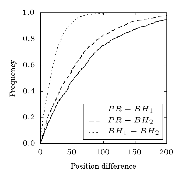
(a) Network of size 1000

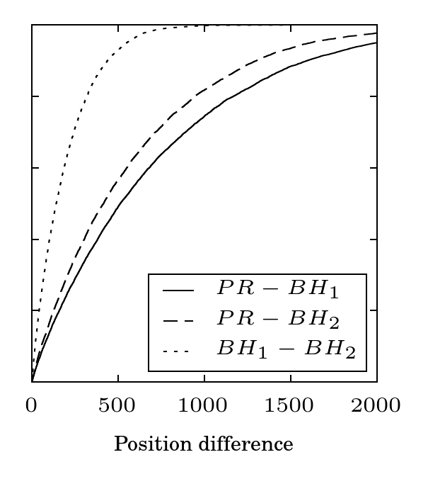
(b) Network of size 10000

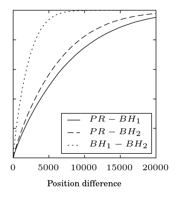
(c) Network of size 100000

Figure 4: Comparison of the empirical CDF of the absolute rank position difference (Erdős-–Rényi networks)

In Figure 4 we show the results of both steps of the simulation of the three Erdős-–Rényi networks. Note that the network size does not affect the shape of the curves; they are very similar for all three network instances. Moreover, the $PR-BH_{2}$ curve is always above the $PR-BH_{1}$ curve, which means that the $BH_{2}$ result set nearer to the $PR$ result set than $BH_{1}$ is. This can be explained if we look at the arc weights: $BH_{1}$ comes from a network where the overall weights are lower than $BH_{2}$. In a network with lower weights, the black hole steady-state probability is higher, which means that it is more likely that a random walker, from any node, moves to the black hole. But the black hole is a sink so the random walker will teleport after reaching it. This means that the black hole has an higher steady-state probability, and the teleportation effect is amplified.

As specified above, the PageRank result sets are identical in both simulation steps meaning that the PageRank metric fails to capture the effect induced by the different weight distribution. The dotted curve $BH_{1}-BH_{2}$ highlights that the two result sets $BH_{1}$ and $BH_{2}$ are always different. Note that this curve is steeper than same curve related to the other two sets, because the difference among the two result sets $BH_{1}$ and $BH_{2}$ is overall less than the difference between either $BH_{1}$ or $BH_{2}$ and $PR$.

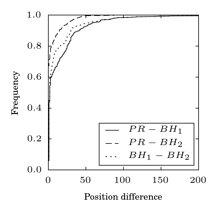
(a) Network of size 1000

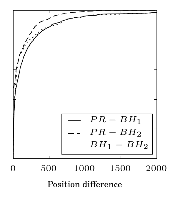
(b) Network of size 10000

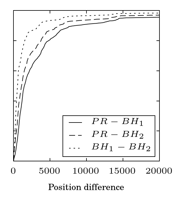
(c) Network of size 100000

Figure 5: Comparison of the empirical CDF of the absolute rank position difference (scale-free networks)

Figure 5 compares the result sets related to the three scale-free network. The network size of scale-free networks does not influence much the shape of the curves, however both $PR-BH_{1}$ and $PR-BH_{2}$ get smoother when the network increases in size. Despite this difference, the curve $PR-BH_{2}$ keeps staying above the curve $PR-BH_{1}$, meaning that the Black Hole metric assesses the difference in wariness of the nodes even in scale-free networks. Finally, the two result sets $BH_{1}$ and $BH_{2}$ exhibit different behaviour when the network size grows: the curve $BH_{1}-BH_{2}$ is between the other two curves when size is 1000, it almost coincides with $PR-BH_{1}$ when size is 10000, it is above the other two curves when size is 100000.

(a) $PR-{BH}_{1}$

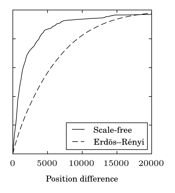
(b) $PR-{BH}_{2}$

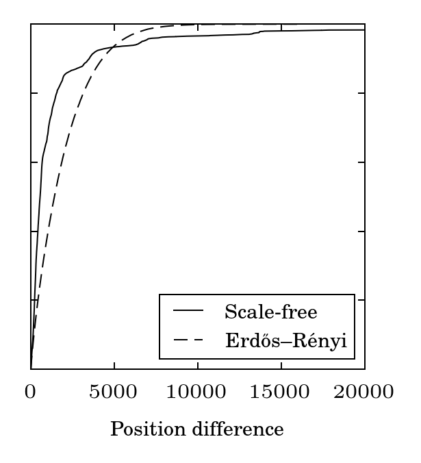
(c) ${BH}_{1}-{BH}_{2}$

Figure 6: Comparison of the empirical CDF of the absolute rank position difference, same size (100k nodes)

At last, in Figure 6 we compare Erdős-–Rényi and scale-free networks of size 100000 by grouping together the curves of the same pair of result sets. Note that the scale-free curves are different than the Erdős-–Rényi curves. This effect may depend on the different topology of the two networks. In scale-free networks, nodes with high indegree, which are few in number, are less affected by the weight fluctuations we introduced with our experiments. Nodes with low indegree, which are more, are instead strongly affected by the weight doubling, and their positions change a lot. This causes the scale-free curves to appear steeper compared to the Erdős-–Rényi curves, although the behaviour of the Black Hole metric remains the same.

The second set of experiments we apply the Black Hole Metric to two real world networks, Advogato and Libimseti.cz, retrieved from [23].

Advogato (www.advogato.org) is an online community platform for free software developers. As reported in the website of Advogato ”Since 1999, our goal has been to be a resource for free software developers around the world, and a research testbed for group trust metrics and other social networking technologies”. Here we consider the Advogato [31] [29] trust network, where nodes are Advogato users and the direct arcs represent trust relationships. Advogato names ”certification” a trust link. There are three different levels of certifications, corresponding to three weights for arcs: apprentice (0.6), journeyer (0.8) and master (1.0). A user with no trust certificate is called an observer. The network consists of 6541 nodes and 51127 arcs and it exhibits an indegree and outdegree power law distribution. As in the previously discussed experiments, we compute on this network the PageRank and the Black Hole Metric and compare them using a cumulative distribution graph, where the x-axis represents the possible absolute rank position difference between the PageRank and the Black Hole Metric of the nodes, while the y-axis represents the cumulative frequency of appearance. To compute Black Hole Metric we set $l_{i}=0.6$ and $h_{i}=1.0$ for all nodes in the network.

Figure 7 shows the results. It is clear that the Black Hole Metric produces different values (and ranks) compared to those computed by using PageRank. In practice, it means that Black Hole Metric produces a different ranking compared to PageRank. For example, in Table 1, we report the rank of the first 10 users of Advogato, computed using the PageRank and Black Hole Metric.

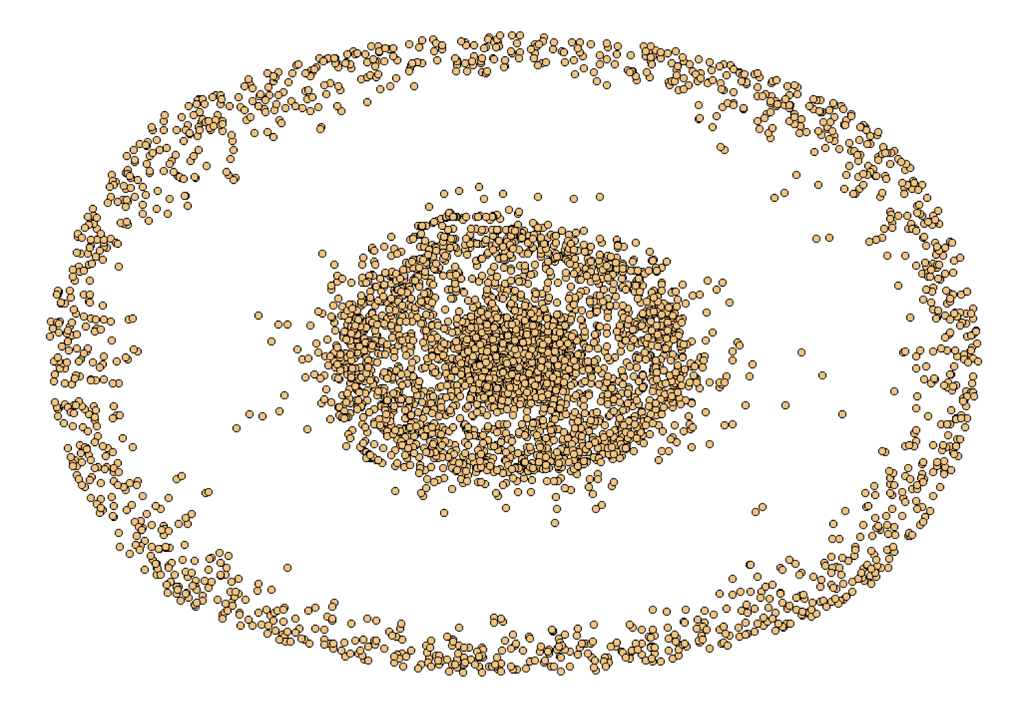
(a) The network.

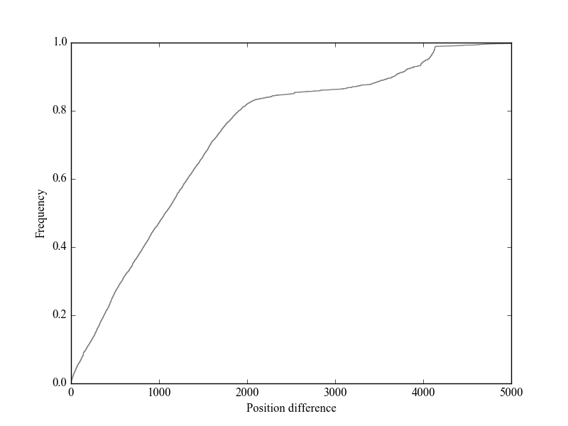
(b) $PR-BH$ CDF.

Figure 7: The Advogato trust network

Rank	PageRank		BlackHole metric
	NodeName	PageRank Value	NodeName	BlackHole Value
1	federico	0.02093458	alan	0.00594131
2	alan	0.00978148	miguel	0.00387012
3	miguel	0.00658376	rms	0.00290212
4	raph	0.00405245	raph	0.00230948
5	rms	0.00381952	federico	0.00176002
6	jwz	0.00274046	jwz	0.00172800
7	davem	0.00262117	rasmus	0.00158964
8	rth	0.00258019	rth	0.00158964
9	rasmus	0.00250191	gstein	0.00138078
10	gstein	0.00230680	davem	0.00135993

Table 1: Rank of the first 10 users of Advogato trust network computed by using PageRank and Black Hole Metric.

As reported in the website of Advogato, in order to assess the certification level of each user they use a basic trust metric computed relatively to a ”seed” of trusted accounts. The original four trust metric seeds, set in 1999 when Advogato went online, were: $raph$ (Raph Levien), $miguel$ (Miguel Icaza), $federico$ (Federico Mena-Quntero) and $alan$ (Alan Cox). In 2007 $mako$ (Benjamin Mako Hill) replaced $federico$. As we can infer from Table 1 both metrics are somewhat able to capture the important role covered by the Advogato trust metric seeds, by putting them in the top positions. However, Black Hole Metric, in our opinion, produces a more appropriate ranking, according to the following observations:

• $federico$ is first according to PageRank, while is 5th according to Black Hole Metric. Moreover the PageRank $federico$’s value is also significantly higher compared to $alan$ (the second in the chart), which means that $federico$ is steadly in the first position with a wide margin, despite the fact that he has not been a seed since 2007. We believe that lower position that the Black Hole Metric assigns to $federico$ better captures the fact that he was swapped out of the seed set.

• Another interesting difference is about the different position of the node $mako$. It is ranked 257^th by the PageRank and 142^th by Black Hole Metric. This ranking difference suggest that the Black Hole Metric better captures the relevance that $mako$ has been assuming inside the Advogato community.

6 Conclusion and future works

In this article, we proposed a new PageRank based metric called Black Hole Metric which aims at solving the normalization issue of PageRank algorithm. We provided examples that highlight these problems and show that Black Hole Metric provides a different ranking that takes into account the relative weights of the node outlinks. We formally defined Black Hole Metric proving that it is an extension of PageRank. We also compared the computational complexity of Black Hole Metric and PageRank proving that they are quite similar. We proved that the Black Hole Metric always converges. Finally, we experimented with the metric on several different networks and showed first results, suggesting that the Black Hole metric seems to capture particular nodes behaviours; this actually deserves further investigation in order to assess Black Hole Metric semantics, and how it can help to model and address the ranking problem in different contexts. In addition to this issue, others must be addressed.

In paragraph 4.3 we said that the black hole rank value is meaningless for the node ranking. Is the black hole just a mathematical trick used to guarantee the stochasticity of the link matrix or does it have an additional meaning? It is clear that the higher the PageRank of the black hole is, the more the nodes of the network do not trust each other. It would be interesting to study the possible correlation between the lack of trust of the nodes and the position or value of the black hole in the Black Hole Metric ranking.

Another open issue concerns the security of Black Hole Metric. We did not investigate possible vulnerabilities of the metric, as they were not the focus of this article. How does the Black Hole Metric behave in a network where security considerations are important? Does it guarantee protection against common and uncommon attacks by internal or external agents [10]?

At last, in this article we did not investigate about methods and algorithms to practically compute the steady-state probability vector. Black Hole Metric can be seen as a generalization of PageRank and as such, many of the algorithms that compute PageRank could be adapted to work with Black Hole Metric. It would be interesting to find out to what extent is it possible to reuse existing PageRank computation methods in order to improve the applicability of the Black Hole Metric.

References

- [1] Donovan Artz and Yolanda Gil. A survey of trust in computer science and the semantic web. Web Semantics: Science, Services and Agents on the World Wide Web, 5(2):58–71, 2007.
- [2] Bahman Bahmani, Kaushik Chakrabarti, and Dong Xin. Fast personalized pagerank on mapreduce. In Proceedings of the 2011 ACM SIGMOD International Conference on Management of Data, SIGMOD ’11, pages 973–984, New York, NY, USA, 2011. ACM.
- [3] Bahman Bahmani, Abdur Chowdhury, and Ashish Goel. Fast incremental and personalized pagerank. Proc. VLDB Endow., 4(3):173–184, December 2010.
- [4] Punam Bedi and Pooja Vashisth. Empowering recommender systems using trust and argumentation. Information Sciences, 279:569–586, 2014.
- [5] Pavel Berkhin. A survey on pagerank computing. Internet Mathematics, 2(1), 2005.
- [6] Monica Bianchini, Marco Gori, and Franco Scarselli. Inside pagerank. ACM Trans. Internet Technol., 5(1):92–128, Febraury 2005.
- [7] Béla Bollobás, Christian Borgs, Jennifer Chayes, and Oliver Riordan. Directed scale-free graphs. In Proceedings of the Fourteenth Annual ACM-SIAM Symposium on Discrete Algorithms, SODA ’03, pages 132–139, Philadelphia, PA, USA, 2003. Society for Industrial and Applied Mathematics.
- [8] S. Brin and L. Page. The anatomy of a large-scale hypertextual web search engine. In Seventh International World-Wide Web Conference (WWW 1998), 1998.
- [9] Vincenza Carchiolo, Alessandro Longheu, and Michele Malgeri. Reliable peers and useful resources: Searching for the best personalised learning path in a trust- and recommendation-aware environment. Information Sciences, 180(10):1893 – 1907, 2010. Special Issue on Intelligent Distributed Information Systems.
- [10] Vincenza Carchiolo, Alessandro Longheu, Michele Malgeri, and Giuseppe Mangioni. Trusting evaluation by social reputation. In Intelligent Distributed Computing, Systems and Applications, Proceedings of the 2nd International Symposium on Intelligent Distributed Computing - IDC 2008, pages 75–84. Springer, 2008.
- [11] Vincenza Carchiolo, Alessandro Longheu, Michele Malgeri, and Giuseppe Mangioni. Gain the Best Reputation in Trust Networks, pages 213–218. Springer Berlin Heidelberg, Berlin, Heidelberg, 2012.
- [12] Vincenza Carchiolo, Alessandro Longheu, Michele Malgeri, and Giuseppe Mangioni. Trust assessment: a personalized, distributed, and secure approach. Concurrency and Computation: Practice and Experience, 24(6):605–617, 2012.
- [13] Vincenza Carchiolo, Alessandro Longheu, Michele Malgeri, and Giuseppe Mangioni. Users attachment in trust networks: Reputation vs. effort. Int. J. Bio-Inspired Comput., 5(4):199–209, July 2013.
- [14] Vincenza Carchiolo, Alessandro Longheu, Michele Malgeri, and Giuseppe Mangioni. Searching for experts in a context-aware recommendation network. Computers in Human Behavior, 51:1086 – 1091, 2015. Computing for Human Learning, Behaviour and Collaboration in the Social and Mobile Networks Era.
- [15] Li Chen, Guanliang Chen, and Feng Wang. Recommender systems based on user reviews: The state of the art. User Modeling and User-Adapted Interaction, 25(2):99–154, June 2015.
- [16] N. L. Chervany D. H. McKnight. The meanings of trust. Technical report, Minneapolis, USA, 1996.
- [17] Paul Erdős and Alfréd Rényi. On random graphs i. Publicationes Mathematicae (Debrecen), 6:290–297, 1959 1959.
- [18] David F. Gleich. Pagerank beyond the web. CoRR, abs/1407.5107, 2014.
- [19] Pankaj Gupta, Ashish Goel, Jimmy Lin, Aneesh Sharma, Dong Wang, and Reza Zadeh. Wtf: The who to follow service at twitter. In Proceedings of the 22Nd International Conference on World Wide Web, WWW ’13, pages 505–514, Republic and Canton of Geneva, Switzerland, 2013. International World Wide Web Conferences Steering Committee.
- [20] Sepandar D. Kamvar, Mario T. Schlosser, and Hector Garcia-Molina. The EigenTrust algorithm for reputation management in P2P networks. In Proceedings of the Twelfth International World Wide Web Conference, 2003., 2003.
- [21] Young Ae Kim and Rasik Phalak. A trust prediction framework in rating-based experience sharing social networks without a web of trust. Information Sciences, 191:128–145, 2012.
- [22] Jon M. Kleinberg. Authoritative sources in a hyperlinked environment. Journal of ACM, 46(5):604–632, 1999.
- [23] Jérôme Kunegis. KONECT – The Koblenz Network Collection. In Proc. Int. Conf. on World Wide Web Companion, pages 1343–1350, 2013.
- [24] Amy N. Langville and Carl D. Meyer. Deeper inside pagerank. Internet Mathematics, 1:2004, 2004.
- [25] HyunChul Lee and Allan Borodin. Perturbation of the hyper-linked environment. In Tandy Warnow and Binhai Zhu, editors, Computing and Combinatorics, volume 2697 of Lecture Notes in Computer Science, pages 272–283. Springer Berlin Heidelberg, 2003.
- [26] HyunChul Lee and Allan Borodin. Perturbation of the hyper-linked environment. In Tandy Warnow and Binhai Zhu, editors, Computing and Combinatorics, volume 2697 of Lecture Notes in Computer Science, pages 272–283. Springer Berlin Heidelberg, 2003.
- [27] R. Lempel and S. Moran. Salsa: The stochastic approach for link-structure analysis. ACM Trans. Inf. Syst., 19(2):131–160, April 2001.
- [28] S. Marsh. Formalising Trust as a Computational Concept. PhD thesis, 1994.
- [29] Paolo Massa, Martino Salvetti, and Danilo Tomasoni. Bowling alone and trust decline in social network sites. In Proc. Int. Conf. Dependable, Autonomic and Secure Computing, pages 658–663, 2009.
- [30] Marc A. Najork. Comparing the effectiveness of hits and salsa. In Proceedings of the Sixteenth ACM Conference on Conference on Information and Knowledge Management, CIKM ’07, pages 157–164, New York, NY, USA, 2007. ACM.
- [31] Advogato network dataset KONECT, January 2016.
- [32] Lawrence Page, Sergey Brin, Rajeev Motwani, and Terry Winograd. The pagerank citation ranking: Bringing order to the web. Technical Report 1999-66, Stanford InfoLab, November 1999. Previous number = SIDL-WP-1999-0120.
- [33] S. Prabha, K. Duraiswamy, and J. Indhumathi. Comparative analysis of different page ranking algorithms. International Journal of Computer, Electrical, Automation, Control and Information Engineering, 8(8):1486 – 1494, 2014.
- [34] Luca Pretto. A theoretical analysis of google’s pagerank. In AlbertoH.F. Laender and ArlindoL. Oliveira, editors, String Processing and Information Retrieval, volume 2476 of Lecture Notes in Computer Science, pages 131–144. Springer Berlin Heidelberg, 2002.
- [35] Mathew Richardson and Pedro Domingos. The Intelligent Surfer: Probabilistic Combination of Link and Content Information in PageRank. In Advances in Neural Information Processing Systems 14. MIT Press, 2002.
- [36] Antonio J. Roa-Valverde and Miguel-Angel Sicilia. A survey of approaches for ranking on the web of data. Inf. Retr., 17(4):295–325, August 2014.
- [37] Sini Ruohomaa and Lea Kutvonen. Trust management survey. In proceedings of ITRUST 2005, number 3477 in LNCS, pages 77–92. Springer-Verlag, 2005.
- [38] P. Sargolzaei and F. Soleymani. Pagerank problem, survey and future research directions. 5(19):937–956, 2010.
- [39] Upul Senanayake, Mahendra Piraveenan, and Albert Zomaya. The pagerank-index: Going beyond citation counts in quantifying scientific impact of researchers. PLoS ONE, 10(8):e0134794, 08 2015.
- [40] Jesus Serrano-Guerrero, Enrique Herrera-Viedma, José Olivas, Andres Cerezo, and Francisco Romero. A google wave-based fuzzy recommender system to disseminate information in university digital libraries 2.0. Information Sciences, 181:1503–1516, 05 2011.
- [41] Jesus Serrano-Guerrero, Francisco Romero, and José Olivas. Hiperion: A fuzzy approach for recommending educational activities based on the acquisition of competences. Information Sciences, pages –, 11 2013.
- [42] Ashutosh Kumar Singh and Ravi Kumar P. A comparative study of page ranking algorithms for information retrieval. 3(4):745 – 756, 2009.
- [43] Xuanhui Wang, Tao Tao, Jian-Tao Sun, Azadeh Shakery, and Chengxiang Zhai. Dirichletrank: Solving the zero-one gap problem of pagerank. ACM Transactions on Information Systems, 26(2):1–29, 2008.
- [44] Wenpu Xing and A. Ghorbani. Weighted pagerank algorithm. In Communication Networks and Services Research, 2004. Proceedings. Second Annual Conference on, pages 305–314, May 2004.
- [45] Li Xiong and Ling Liu. Peertrust: Supporting reputation-based trust for peer-to-peer electronic communities. IEEE Trans. on Knowl. and Data Eng., 16(7):843–857, July 2004.
- [46] A. O. Zhirov, O. V. Zhirov, and D. L. Shepelyansky. Two-dimensional ranking of wikipedia articles. CoRR, abs/1006.4270, 2010.
- [47] Runfang Zhou and Kai Hwang. Powertrust: A robust and scalable reputation system for trusted peer-to-peer computing. IEEE Trans. Parallel Distrib. Syst., (4):460–473.
- [48] Yangbo Zhu and Xing Li. Distributed pagerank computation based on iterative aggregation-disaggregation methods. In Proceedings of the 14th ACM international conference on Information and knowledge management, pages 578–585, 2005.