Hierarchical multi-stage MCMC follow-up of continuous gravitational wave candidates

Abstract

Leveraging Markov chain Monte Carlo (MCMC) optimization of the $\mathcal{F}$-statistic, we introduce a method for the hierarchical follow-up of continuous gravitational wave candidates identified by wide-parameter space semi-coherent searches. We demonstrate parameter estimation for continuous wave sources and develop a framework and tools to understand and control the effective size of the parameter space, critical to the success of the method. Monte Carlo tests of simulated signals in noise demonstrate that this method is close to the theoretical optimal performance.

I Introduction

A target for the advanced gravitational wave detector network of LIGO (Aasi et al., 2015) and Virgo (Acernese et al., 2015) are long-lived quasi-periodic continuous gravitational waves from neutron stars. Detection of such signals would provide unique astrophysical insights and has hence motivated numerous searches (Abbott et al., 2017a, b, c, d, e, 2017).

The gravitational wave signal strain from a rotating neutron star $h(t,\boldsymbol{\mathcal{A}},\boldsymbol{\mathbf{\lambda}})$ (Jaranowski et al., 1998) has two distinct sets of parameters: $\boldsymbol{\mathcal{A}}{=}\{h_{0},\cos\iota,\psi,\phi_{0}\}$, a set of the four amplitude parameters and $\boldsymbol{\mathbf{\lambda}}$, a set of the phase-evolution parameters consisting of the sky-location, frequency $f$, any spin-down terms $\{\dot{f},\ddot{f},\ldots\}$ and binary orbital parameters, if required (see Prix (2009) for a review).

CW searches are often based on a fully coherent matched-filtering method whereby a template for $h(t;\boldsymbol{\mathcal{A}},\boldsymbol{\mathbf{\lambda}})$ is convolved against the data, resulting in a detection statistic. Four search categories can be identified dependent on the level of prior knowledge about certain parameters: targeted searches for a signal from a known pulsar where the phase-evolution parameters are considered known; an extension to targeted searches are narrow-band searches which allow some uncertainty in the frequency and its derivatives; directed searches in which the sky-location is considered known, but not the other phase evolution parameters (i.e., searching for the neutron star in a supernova remnant which does not have a known pulsar); and all-sky searches where none of the phase-evolution parameters are known. Unknown parameters must be searched over either numerically using a template bank, or analytically maximized.

Wide-parameter space searches (directed or all-sky) often use a semi-coherent search because at fixed computing cost it is typically more sensitive to unknown signals than a fully coherent search (Brady et al., 1998; Prix and Shaltev, 2012; Prix, 2009). Generically speaking, a semi-coherent search involves dividing the total observation span $T$ into $N_{\mathrm{\rm seg}}$ segments, in each segment computing a fully coherent detection statistic, then recombining the detection statistic in each segment into a semi-coherent detection statistic; for details of specific variations on this principle, see (Brady and Creighton, 2000; Krishnan et al., 2004; Astone et al., 2014; Abbott et al., 2008; Pletsch and Allen, 2009; Pletsch, 2008).

The result of a semi-coherent wide-parameter space search is a list of any candidates which pass a predefined detection threshold. To further vet these candidates, they are subjected to a hierarchical follow-up: a process of increasing the coherence time, eventually aiming to calculate a fully coherent detection statistic over the maximal span of data. In essence, the semi-coherent search is powerful in detecting unknown signals as it spreads the significance of a candidate over a wider area of parameter space allowing for a sparser template covering. Subsequently, the follow-up attempts to reverse this process and recover the maximum significance and tightly constrain the candidate parameters (cf. Section V for an illustration and introduction to other hierarchical follow-up methods). In this work, we propose a hierarchical follow-up procedure using MCMC optimization.

MCMC optimization has been used in parameter estimation for gravitational waves from compact binary coalescence events (Christensen and Meyer, 1998, 2001; Christensen et al., 2004a; Röver et al., 2006; Veitch et al., 2015). For the problem of detecting CWs, MCMC-based methods have been developed for directed searches with unknown frequency and spin-down (Christensen et al., 2004b; Umstätter et al., 2004). In Veitch (2007), a method was developed and applied for a directed search for CWs from Supernova remnant 1987A and more recently for CWs from known pulsars (Abbott et al., 2010) (since this time, an improved nested sampling based approach has instead been used for known pulsars (Pitkin et al., 2012, 2017; Abbott et al., 2017a)).

MCMC searches for simulated CW signals using these methods converge to the correct solution in a reasonable amount of time, provided the volume of parameter space occupied by a signal (a concept we define in Section IV.2) is a significant fraction of the total prior volume. When this is not the case, convergence becomes problematic; Umstätter (2006) discussed this in the context of frequency and spin-down uncertainty, but uncertainties in sky location will cause similar issues.

In this work, we provide methods to understand the conditions under which MCMC searches are effective. We then apply this to develop a follow-up method for candidates from semi-coherent wide-parameter space searches.

We begin in Section II with a description of MCMC samplers and then discuss how these can be used in CW searches in Section III. In Section IV we introduce methods to understand the conditions for which an MCMC search is suitable before describing and testing the follow-up procedure in Section V. Finally, in Section VI we give a timing model to predict computing costs before concluding in Section VII.

The methods introduced in this paper have been implemented in the open source python package pyfstat (Ashton, 2017). Source code along with all examples in this work can be found at https://gitlab.aei.uni-hannover.de/GregAshton/PyFstat.

II MCMC samplers

Given some data $\boldsymbol{x}$ and a hypothesis $\mathcal{H}$ about the generative model which produced the data, we can infer the posterior distribution for the set of model parameters $\theta$ from Bayes theorem

$$P(\theta|\boldsymbol{x},\mathcal{H})=\frac{P(\boldsymbol{x}|\theta,\mathcal{H})P(\theta|\mathcal{H})}{P(\boldsymbol{x}|\mathcal{H})}\,.$$ (1)

In this expression, $P(\boldsymbol{x}|\theta,\mathcal{H})$ is the likelihood of observing the data for the generative model at hand, $P(\theta|\mathcal{H})$ is the prior probability distribution for the model parameters, and $P(\boldsymbol{x}|\mathcal{H})$ is a normalization constant.

For many problems, it is not possible to solve Eq. (1) analytically. MCMC algorithms provide a means to instead sample from $P(\theta|\boldsymbol{x},\mathcal{H})$, the posterior distribution, allowing inferences about the model parameters to be made using these samples. Since the normalization constant is independent of $\theta$, it is only necessary to sample from the unnormalized distribution, i.e.,

$$P(\theta|\boldsymbol{x},\mathcal{H})\propto P(\boldsymbol{x}|\theta,\mathcal{H})P(\theta|\mathcal{H})\,.$$ (2)

In the rest of this Section, we introduce the details of the MCMC sampler used in this investigation. For a general introduction to MCMC samplers, see, e.g., MacKay (2003) or Gelman et al. (2013).

II.1 The ptemcee sampler

In this work we use the ptemcee MCMC ensemble sampler (Vousden et al., 2016; Foreman-Mackey et al., 2013), an implementation of the affine-invariant ensemble sampler proposed by Goodman and Weare (2010). This choice addresses a key issue with the use of MCMC samplers, the choice of proposal distribution. At each step of the MCMC algorithm, the sampler generates from a proposal distribution a jump to a new point in parameter space. Usually, this proposal distribution must be “tuned” so that the MCMC sampler efficiently walks the parameter space without either jumping too far, or taking such small steps that it takes a long time to traverse the peak (MacKay, 2003; Gelman et al., 2013).

Ensemble samplers use a number of parallel walkers. The proposal jump for each walker is generated by the stretch move (see Goodman and Weare (2010)): the new position is determined by the position of a complementary walker from the ensemble and a scaling variable. The scaling variable is a random variable, for the particular form used here see Foreman-Mackey et al. (2013), with a single proposal scale parameter. This scale parameter does not require tuning and can typically be left at its default value. As such, ensemble samplers do not use a proposal distribution which requires tuning; in effect the proposal is determined by the position of the others walkers in the ensemble.

Moreover, by applying an affine transformation, the efficiency of the algorithm is not diminished when the parameter space is highly anisotropic. Aside from the parallel tempering functionality (which we discuss momentarily), this sampler has three tuning parameters: a proposal scale, the number of walkers $N_{w}$, and the number of steps to take. For the number of walkers, it is recommended (Foreman-Mackey et al., 2013) to use as many as possible (limited by memory constrains); for our purposes we typically find that $N_{w}=100$ is sufficient. We will discuss the number of steps in Section II.3.

When setting up an ensemble MCMC sampler, one must also consider how to initialize the sampler, choosing the initial parameter values for each walker. Typically, we want to explore the entire prior parameter space and therefore the initial position of each walker can be selected by a random draw from the prior distribution. However, instances do occur when one would like to initialize the walkers from a different distribution, e.g., if a search has already been performed and the signal localized to a small region of the prior volume and one would solely like to perform parameter estimation.

II.2 Parallel tempering: sampling multimodal posteriors

Beyond the standard ensemble sampler, the ptemcee sampler also uses parallel-tempering. A parallel tempered MCMC sampler (Swendsen and Wang, 1986) runs $N_{t}$ simulations in parallel with the likelihood in the $i\mathrm{th}$ simulation raised to a power $1/t_{i}$, where $t_{i}$ is referred to as the temperature. Eq. (2) for the $i$th temperature is then rewritten as

$$P(\theta|\boldsymbol{x},t_{i},\mathcal{H})\propto P(\boldsymbol{x}|\theta,\mathcal{H})^{1/t_{i}}P(\theta|\mathcal{H})\,.$$ (3)

Setting $t_{0}=1$ with $t_{i}>t_{0}\;\forall\;i>0$, such that the $i=0$ temperature recovers Eq. (2) while for higher temperatures the likelihood is broadened. During the simulation, the algorithm swaps the position of the walkers between the different temperatures. This allows the $t_{0}$ walkers (from which we draw samples of the posterior) to efficiently sample from a multimodal posterior. This method introduces additional tuning parameters for the choice of temperatures. Unless stated otherwise, all examples in this work use a default setup: 3 temperatures logarithmically spaced between ${\color[rgb]{0,0,0}1}$ and ${\color[rgb]{0,0,0}10^{0.5}}$. In testing (see for example Section IV.4) this was found to be efficient over a range of searches. ptemcee also implements a dynamical temperature selection algorithm (Vousden et al., 2016) which will update the temperature ladder during the sampling.

II.3 Assessing convergence and independent samples

In tuning the number of steps taken by a Markov chain there are two distinct issues to address: initialization bias and autocorrelation in equilibrium (Sokal, 1997).

i) The first of these issues refers to the initial transient period which occurs whilst the Markov chain (in our case, the MCMC sampler) transitions from the initialization distribution to the posterior distribution. To remove any bias, samples taken during this period, referred to as the burn-in, are discarded from the set of samples used to infer the posterior. An example of this burn-in period can be seen later in Fig. 1. The difficulty lies in deciding how many burn-in steps are required, values of $\mathcal{O}(10^{2}-10^{4})$ steps are typical in the literature. In most cases, $N_{\mathrm{\rm burn}}$, the number of burn-in steps, is predetermined and a graphical check of the MCMC samples can be performed to ensure the validity of the results. To determine the number of burn-in steps needed, Sokal (1997) defines the exponential autocorrelation time $\tau_{\mathrm{exp}}$, the relaxation time of the slowest mode of the system, and recommends that “$20\tau_{\mathrm{exp}}$ burn-in samples are usually more than adequate”.

ii) The second issue, is that once the sampler has reached equilibrium it will draw samples from the posterior distribution (we refer to these are the production samples), but these samples are not independent, they are correlated with an integrated autocorrelation time $\tau_{\textrm{int}}$ (Sokal, 1997). The effective number of independent samples from a simulation with $N_{\mathrm{\rm prod}}$ production samples is then roughly $N_{\mathrm{\rm prod}}/2\tau_{\mathrm{int}}$.

The total number of steps taken by the sampler is the sum of $N_{\mathrm{\rm burn}}$ and $N_{\mathrm{\rm prod}}$.

Usually, $\tau_{\mathrm{exp}}$ and $\tau_{\mathrm{int}}$ are of the same order of magnitude (Sokal, 1997). Therefore, we will use the emcee estimator for the integrated autocorrelation (see Foreman-Mackey et al. (2013)) time which we refer to simply as the autocorrelation time (ACT). In future work, we plan to explore the method proposed by Akeret et al. (2013) and Allison and Dunkley (2014) to estimate $\tau_{\mathrm{exp}}$ from a least-squares fit to the autocorrelation function and also to investigate stopping criteria. In Section III.3 and Section VI, we will provide estimates for the ACT in the context of CW searches.

The methods discussed here are part of a broader literature on assessing convergence. We have chosen to use the autocorrelation time following the recomendations given in Foreman-Mackey et al. (2013), but alternatives such as the method proposed by Raftery and Lewis (1991) could also be applied. For a broad review and general discussion of convergence, see Cowles and Carlin (1996) and Hogg and Foreman-Mackey (2017).

III MCMC and the ${\mathcal{F}}$-statistic

In this section, we give a brief introduction to the application of the ${\mathcal{F}}$-statistic in a hypothesis testing framework and then show how this can be used in a CW MCMC search.

III.1 Hypothesis testing framework: fully coherent

In Prix and Krishnan (2009), a framework was introduced demonstrating the use of the ${\mathcal{F}}$-statistic (Jaranowski et al., 1998; Cutler and Schutz, 2005) in defining the Bayes factor,

$$B_{\rm S/G}(\boldsymbol{x})\equiv\frac{P(\boldsymbol{x}|\mathcal{H}_{\rm S})}{P(\boldsymbol{x}|\mathcal{H}_{\rm G})}\,,$$ (4)

between the signal hypothesis and the Gaussian noise hypothesis computed on some data $\boldsymbol{x}$; we now briefly review this framework.

The noise hypothesis $\mathcal{H}_{\rm G}$ states that the data $\boldsymbol{x}$ contains only Gaussian noise $\boldsymbol{n}$, while the signal hypothesis $\mathcal{H}_{\rm S}$ states that there is an additive signal in the data, i.e. $\boldsymbol{x}=\boldsymbol{n}+\boldsymbol{s}(\boldsymbol{\mathcal{A}},\boldsymbol{\mathbf{\lambda}})$. As mentioned in the introduction, the signal $\boldsymbol{s}$ is generally expressed as depending on two sets of parameters, namely the four amplitude parameters $\boldsymbol{\mathcal{A}}$, and a number of phase-evolution parameters $\boldsymbol{\mathbf{\lambda}}$, such as the frequency, spindown and sky-position of the source.

With this one obtains an explicit analytic expression (not given here for brevity, e.g. see Prix (2009)) for the likelihood-ratio function, defined as

$$\mathcal{L}(\boldsymbol{x};\boldsymbol{\mathcal{A}},\boldsymbol{\mathbf{\lambda}})\equiv\frac{P(\boldsymbol{x}|\mathcal{H}_{\rm S},\boldsymbol{\mathcal{A}},\boldsymbol{\mathbf{\lambda}})}{P(\boldsymbol{x}|\mathcal{H}_{\rm G})}\,.$$ (5)

Assuming independent priors for the amplitude parameters $\boldsymbol{\mathcal{A}}$ and the phase-evolution parameters $\boldsymbol{\mathbf{\lambda}}$, and noting that $P(\boldsymbol{x}|\mathcal{H}_{\rm G})$ does not depend on these signal parameters, we can express the Bayes factor of Eq. (4) as

$$B_{\rm S/G}(\boldsymbol{x})=\iint\mathcal{L}(\boldsymbol{x};\boldsymbol{\mathcal{A}},\boldsymbol{\mathbf{\lambda}})P(\boldsymbol{\mathcal{A}}|\mathcal{H}_{\rm S})P(\boldsymbol{\mathbf{\lambda}}|\mathcal{H}_{\rm S})\;d\boldsymbol{\mathcal{A}}d\boldsymbol{\mathbf{\lambda}}\,.$$ (6)

It was shown by Prix and Krishnan (2009) (see also Whelan et al. (2014) for a more detailed discussion) that with an appropriate choice of $P(\boldsymbol{\mathcal{A}}|\mathcal{H}_{\rm S})$, the marginalization over the amplitude parameters

$$B_{\rm S/G}(x;\boldsymbol{\mathbf{\lambda}})=\int\mathcal{L}(\boldsymbol{x};\boldsymbol{\mathcal{A}},\boldsymbol{\mathbf{\lambda}})P(\boldsymbol{\mathcal{A}}|\mathcal{H}_{\rm S})\;d\boldsymbol{\mathcal{A}}\,,$$ (7)

can be performed analytically. We refer to the Bayes factor $B_{\rm S/G}(x;\boldsymbol{\mathbf{\lambda}})$ for a fixed value of the phase-evolution parameters $\boldsymbol{\mathbf{\lambda}}$ as a “targeted” Bayes factor. Once $B_{\rm S/G}(\boldsymbol{x};\boldsymbol{\mathbf{\lambda}})$ is computed, the full Bayes factor of Eq. (6) can be calculated by numerical integration over the phase-evolution parameters, i.e.

$$B_{\rm S/G}(\boldsymbol{x})=\int B_{\rm S/G}(\boldsymbol{x};\boldsymbol{\mathbf{\lambda}})P(\boldsymbol{\mathbf{\lambda}}|\mathcal{H}_{\rm S})\;d\boldsymbol{\mathbf{\lambda}}\,.$$ (8)

In this work, we use the amplitude prior choice suggested in Prix et al. (2011), which results in

$$B_{\rm S/G}(\boldsymbol{x};\boldsymbol{\mathbf{\lambda}})\equiv\frac{70}{\hat{\rho}_{\mathrm{max}}^{4}}e^{\widetilde{{\mathcal{F}}}(\boldsymbol{x};\boldsymbol{\mathbf{\lambda}})}\,,$$ (9)

where $\widetilde{{\mathcal{F}}}$ is the fully coherent ${\mathcal{F}}$-statistic. This statistic was originally found (Jaranowski et al., 1998; Cutler and Schutz, 2005) as a frequentist amplitude-maximized likelihood-ratio statistic, i.e.

$$\widetilde{{\mathcal{F}}}(\boldsymbol{x};\boldsymbol{\mathbf{\lambda}})\equiv\max_{\boldsymbol{\mathcal{A}}}\ln\mathcal{L}(\boldsymbol{x};\boldsymbol{\mathcal{A}},\boldsymbol{\mathbf{\lambda}})\,,$$ (10)

which can be expressed in closed analytic form for any given $\boldsymbol{\mathbf{\lambda}}$. The ${\mathcal{F}}$-statistic follows a (non-central) $\chi^{2}_{4}$ distribution with four degrees of freedom, with expectation value

$$E\left[2\widetilde{{\mathcal{F}}}\right]=4+\widetilde{\rho}^{2}\,,$$ (11)

where $\widetilde{\rho}$ defines the coherent signal-to-noise ratio (SNR), and $\widetilde{\rho}^{2}$ is the non-centrality parameter of the $\chi^{2}$ distribution.

We note that the “modified ad-hoc ${\mathcal{F}}$-statistic prior” of Prix et al. (2011) leading to Eq. (9) is somewhat unphysical in that it introduces an arbitrary cutoff $\hat{\rho}_{\mathrm{max}}$ for the signal strength and is not uniform in $\cos\iota$. One could circumvent this by numerically integrating Eq. (8) with physical amplitude priors. However, by using the ${\mathcal{F}}$-statistic instead, we can use fast and mature codes implementing this statistic (namely XLALComputeFstat() (LIGO Scientific Collaboration, 2014)) and thereby greatly improving the speed at which a search can be run with very little loss of detection power (Prix and Krishnan, 2009).

The MCMC class of optimization tools are formulated to solve the problem of inferring the posterior distribution for some general model parameters given some data $\boldsymbol{x}$. In this case, we are concerned with the posterior distribution for $\boldsymbol{\mathbf{\lambda}}$, the phase-evolution parameters which cannot be marginalized analytically. In analogy with Eq. (2), this distribution is given by

$$P(\boldsymbol{\mathbf{\lambda}}|\boldsymbol{x},\mathcal{H}_{\rm S})\propto P(\boldsymbol{x}|\boldsymbol{\mathbf{\lambda}},\mathcal{H}_{\rm S})P(\boldsymbol{\mathbf{\lambda}}|\mathcal{H}_{\rm S})\,.$$ (12)

Dividing through by $P(\boldsymbol{x}|\mathcal{H}_{\rm G})$, we can then write this as

$$P(\boldsymbol{\mathbf{\lambda}}|\boldsymbol{x},\mathcal{H}_{\rm S})\propto B_{\rm S/G}(\boldsymbol{x};\boldsymbol{\mathbf{\lambda}})P(\boldsymbol{\mathbf{\lambda}}|\mathcal{H}_{\rm S})\,.$$ (13)

We use an MCMC algorithm to perform a CW search by applying Eq. (9) as the likelihood along with a prior for the phase-evolution parameters. In this way, the log-likelihood function is proportional to $\widetilde{{\mathcal{F}}}$.

III.2 Hypothesis testing framework: semi-coherent

Eq. (13) is the posterior distribution using a fully coherent statistic (i.e., the log-likelihood is given by $\widetilde{{\mathcal{F}}}$). It was shown by Prix et al. (2011), that the semi-coherent ${\mathcal{F}}$-statistic naturally arises by splitting the likelihood into $N_{\mathrm{\rm seg}}$ independent non-overlapping segments and allowing for independent choices of the amplitude parameters in each segment. Specifically, the semi-coherent targeted Bayes factor is

$$B_{\rm S/G}(\boldsymbol{x};\boldsymbol{\mathbf{\lambda}},N_{\mathrm{\rm seg}})\equiv\left(\frac{70}{\hat{\rho}_{\mathrm{max}}^{4}}\right)^{N_{\mathrm{\rm seg}}}e^{\widehat{{\mathcal{F}}}}\,,$$ (14)

where the semi-coherent ${\mathcal{F}}$-statistic is

$$\widehat{{\mathcal{F}}}\equiv\sum_{\ell=1}^{N_{\mathrm{\rm seg}}}\widetilde{{\mathcal{F}}}(\boldsymbol{x}_{(\ell)};\boldsymbol{\mathbf{\lambda}})\,,$$ (15)

and $\boldsymbol{x}_{(\ell)}$ refers to the data in the $\ell\mathrm{th}$ segment. This semi-coherent ${\mathcal{F}}$-statistic follows again a (non-central) $\chi^{2}$-distribution, but with $4\,N_{\mathrm{\rm seg}}$ degrees of freedom, and non-centrality parameter

$$\widehat{\rho}^{2}=\sum_{\ell=1}^{N_{\mathrm{\rm seg}}}\widetilde{\rho}_{\ell}^{2}\,,$$ (16)

with per-segment SNRs $\widetilde{\rho}_{\ell}$, and expectation

$$E\left[2\widehat{{\mathcal{F}}}\right]=4\,N_{\mathrm{\rm seg}}+\widehat{\rho}^{2}\,.$$ (17)

The posterior distribution for $\boldsymbol{\mathbf{\lambda}}$, Eq. (13), naturally generalizes using a semi-coherent statistic to

$$P(\boldsymbol{\mathbf{\lambda}}|\boldsymbol{x},N_{\mathrm{\rm seg}},\mathcal{H}_{\rm S})\propto B_{\rm S/G}(\boldsymbol{x};\boldsymbol{\mathbf{\lambda}},N_{\mathrm{\rm seg}})P(\boldsymbol{\mathbf{\lambda}}|\mathcal{H}_{\rm S})\,.$$ (18)

and hence can equally be applied in an MCMC algorithm.

One can consider the fully coherent case as a special instance of the semi-coherent case with $N_{\mathrm{\rm seg}}=1$. Any methods developed for parameter estimation using the fully coherent ${\mathcal{F}}$-statistic can easily be generalized to the semi-coherent case. Therefore, in the remainder of this Section, we discuss the general intricacies of setting up and running an MCMC search using the simpler fully coherent ${\mathcal{F}}$-statistic. In Section V, we turn to the primary goal of this paper, the hierarchical multi-stage follow-up of candidates found in semi-coherent searches.

III.3 Example: fully coherent MCMC optimization for a signal in noise

In order to familiarize the reader with the features of an MCMC-CW search, we will now describe a simple directed search (over $f$ and $\dot{f}$) for a simulated signal in 100 days of Gaussian-noise data. The signal is generated with an amplitude ${\color[rgb]{0,0,0}1.0{\times}10^{-24}}$ while for the Gaussian noise $\sqrt{S_{\rm n}}={\color[rgb]{0,0,0}1.0{\times}10^{-23}}$ Hz^-1/2(at the fiducial frequency of the signal), such that the signal has a sensitivity depth of

$$\mathcal{D}\equiv\frac{\sqrt{S_{\rm n}}}{h_{0}}={\color[rgb]{0,0,0}10.0}\,\mathrm{Hz}^{-1/2}\,.$$ (19)

The remaining signal parameters are chosen randomly and labeled $\boldsymbol{\mathbf{\lambda}}^{\mathrm{s}}$ and $\boldsymbol{\mathcal{A}}^{\mathrm{s}}$ such that the simulated frequency and spin-down values are $f^{\mathrm{s}}$ and $\dot{f}^{\mathrm{s}}$; we also choose the reference time to coincide with the middle of the data span.

First, we must define a prior for each search parameter. Typically, we use either a uniform prior bounding the area of interest, but a more informative distribution centered on the target with some uncertainty could also be used. For this example, we use a uniform prior with a frequency range of $\Delta f={\color[rgb]{0,0,0}2.0{\times}10^{-7}}$ Hz and a spin-down range of $\Delta\dot{f}={\color[rgb]{0,0,0}1.8{\times}10^{-13}}$ Hz/s both centered on the simulated signal frequency and spin-down rate. These values were chosen such that the approximate number of unit-mismatch templates is $\mathcal{N}^{*}\approx{\color[rgb]{0,0,0}10}$ (defined in Section IV.2), which, as we discuss in Section IV.4, is sufficiently small to ensure the MCMC search is effective.

Having defined the prior, we initialize the positions of the ${\color[rgb]{0,0,0}100}$ walkers randomly from the prior. The final setup step is to define the number of burn-in and production steps the sampler should take; this is a tuning parameter of the MCMC algorithm, but should be informed by the maximum ACT (see Sec. II.3). For this example, we find this to be $\sim{\color[rgb]{0,0,0}30}$, so to ensure the burn-in length is sufficient $N_{\mathrm{\rm burn}}\gtrsim{\color[rgb]{0,0,0}300}$ (i.e., 10 times the ACT), while to generate $\sim{\color[rgb]{0,0,0}1000}$ independent samples, we need each walker to perform $N_{\mathrm{\rm prod}}={\color[rgb]{0,0,0}300}$ steps.

Using these choices, the simulation is run. To illustrate the full MCMC process, in Fig. 1 we plot the progress of all 100 individual walkers (each represented by an individual line) as a function of the total number of steps. The portion of steps to the left of the dashed vertical line are burn-in samples (see Section II.3) and hence discarded. From this plot we see why: the walkers are initialized from the uniform prior and initially spend some time exploring the whole parameter space before converging. The production samples from the converged region, those to the right of the dashed vertical line, can be used to generate summary statistics or posterior plots.

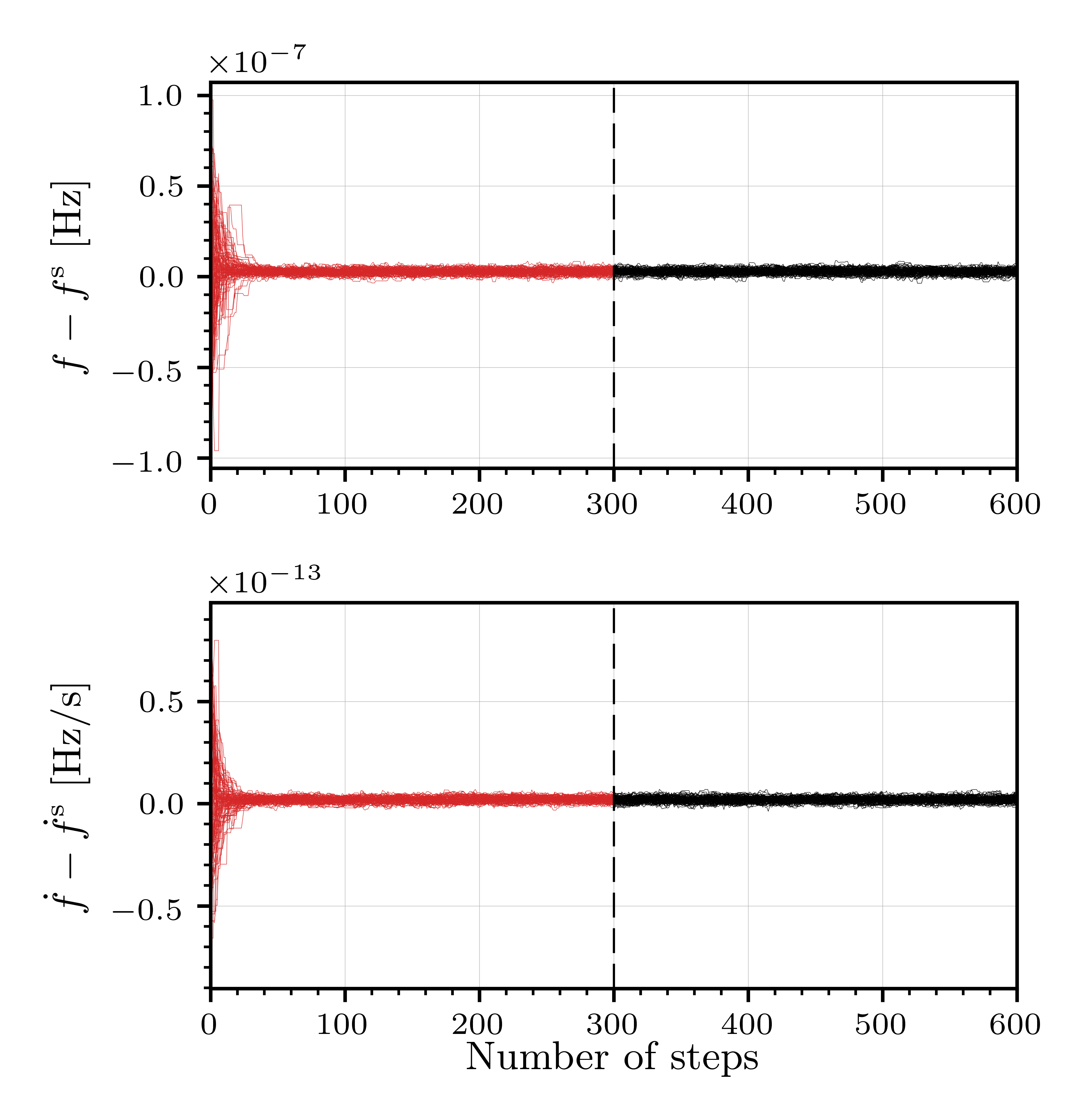
Figure 1: The progress of each walker in the MCMC simulation for a simulated signal in Gaussian noise, searching over a small directed search parameter space: the approximate number of unit-mismatch templates, defined in Section IV.2, is $\mathcal{N}^{*}\approx{\color[rgb]{0,0,0}10}$.

IV Understanding the search space

In general, MCMC samplers are highly effective in generating samples of the posterior in multi-dimensional parameter spaces. However, they will perform poorly if the volume occupied by the signal is small compared to the prior volume; in this Section we define exactly what is meant by this for CW searches.

IV.1 The metric

In a traditional CW search that uses a template bank, the spacing of the grid are chosen such that the loss of relative SNR is bounded. The optimal choice of grid then consists of minimizing the computing cost while respecting this bound (Pletsch, 2010; Prix and Shaltev, 2012; Wette and Prix, 2013; Wette, 2015). We now discuss how the work on setting up these grids can be applied to the problem of determining whether the setup is appropriate for an MCMC method.

For an ${\mathcal{F}}$-statistic search on data containing a signal with phase-evolution parameters $\boldsymbol{\mathbf{\lambda}}^{\mathrm{s}}$, we define the mismatch $\mu$ at a template point $\boldsymbol{\mathbf{\lambda}}$ as

$$\mu(\boldsymbol{\mathbf{\lambda}}^{\mathrm{s}},\boldsymbol{\mathbf{\lambda}})\equiv\frac{\rho^{2}(\boldsymbol{\mathbf{\lambda}}^{\mathrm{s}};\boldsymbol{\mathbf{\lambda}}^{\mathrm{s}})-\rho^{2}(\boldsymbol{\mathbf{\lambda}}^{\mathrm{s}};\boldsymbol{\mathbf{\lambda}})}{\rho^{2}(\boldsymbol{\mathbf{\lambda}}^{\mathrm{s}};\boldsymbol{\mathbf{\lambda}}^{\mathrm{s}})}\in[0,1]\,,$$ (20)

where $\rho^{2}(\boldsymbol{\mathbf{\lambda}}^{\mathrm{s}};\boldsymbol{\mathbf{\lambda}})$ is the non-centrality parameter at $\boldsymbol{\mathbf{\lambda}}$, given a signal at $\boldsymbol{\mathbf{\lambda}}^{\mathrm{s}}$; as such $\rho^{2}(\boldsymbol{\mathbf{\lambda}}^{\mathrm{s}};\boldsymbol{\mathbf{\lambda}}^{\mathrm{s}})$ is the perfectly-matched non-centrality parameter, which is generally proportional to the squared SNR (with equality only in the fully coherent case of $N_{\mathrm{\rm seg}}=1$).

For small offsets $\Delta\boldsymbol{\mathbf{\lambda}}\equiv\boldsymbol{\mathbf{\lambda}}-\boldsymbol{\mathbf{\lambda}}^{\mathrm{s}}$ between the template and signal, the mismatch of Eq. (20) can be approximated by Taylor-expanding in small $\Delta\boldsymbol{\mathbf{\lambda}}$, defining the metric mismatch (Owen, 1996; Balasubramanian et al., 1996; Brady et al., 1998) as

$$\mu(\boldsymbol{\mathbf{\lambda}},\Delta\boldsymbol{\mathbf{\lambda}})\equiv g_{ij}\Delta\lambda^{i}\Delta\lambda^{j}+\mathcal{O}\left(\Delta\boldsymbol{\mathbf{\lambda}}^{3}\right)\,,$$ (21)

where $g_{ij}$ is referred to as the metric and provides a measure of distances in parameter space. Generally, Eq. (21) is a good approximation up to $\mu\gtrsim 0.3-0.5$ (Prix, 2007; Wette and Prix, 2013).

In general, no analytic approximation of the full phase-metric exists, although analytic solutions can be found when searching at a single point in sky for the frequency and spin-down components. A numerical approximation was formulated by Wette and Prix (2013) for the fully coherent phase-metric which uses a coordinate transformation, to the so-called reduced supersky metric $\widetilde{g}^{\mathrm{rss}}_{ij}$, which, of significance in the next section, is well-conditioned. In Wette (2015), the work was further generalized to the semi-coherent case $\widehat{g}^{\mathrm{rss}}_{ij}$ when there are $N_{\mathrm{\rm seg}}$ segments; in the following we use this later definition, with the understanding that when $N_{\mathrm{\rm seg}}=1$, $\widehat{g}^{\mathrm{rss}}_{ij}=\widetilde{g}^{\mathrm{rss}}_{ij}$.

IV.2 The number of templates

When constructing a lattice of search templates (a template bank) to cover an $n$-dimensional parameter space $\mathbb{P}$ at a fixed maximal mismatch of $\mu_{0}$, it can be shown (Prix, 2007; Messenger et al., 2009; Brady et al., 1998; Owen, 1996; Owen and Sathyaprakash, 1999) that the required number of templates is given by

$$\mathcal{N}=\theta\mu_{0}^{-n^{\prime}/2}\int_{\mathbb{T}_{n^{\prime}}}\sqrt{\textrm{det}g}\,d^{n^{\prime}}\lambda\,,$$ (22)

where $g_{ij}$ the parameter space metric, $\mathbb{T}_{n^{\prime}}\subseteq\mathbb{P}$ is the $n^{\prime}\leq n$ dimensional space spanned by the template bank, and $\theta$ is the normalized thickness, which depends on the geometric structure of the covering.

A way to understand the “size” of a given parameter space compared to the size a signal would occupy is to define

$$\mathcal{N}^{*}_{n^{\prime}}\equiv\int_{\mathbb{T}_{n^{\prime}}}\sqrt{\textrm{det}g}\,d^{n^{\prime}}\lambda\,,$$ (23)

the approximate number of templates needed to cover the parameter space at a mismatch of unity. It is the approximate number in the sense that we neglect the effects of the normalized thickness, assuming that $\theta=1$. In general, $\theta$ will depend on the geometric structure of a given covering and the number of dimensions (see, e.g., Prix (2007) or Messenger et al. (2009)). Nevertheless, we fix $\theta=1$ in order to give a rough order of magnitude estimate.

A subtle point (Brady and Creighton, 2000; Cutler et al., 2005; Prix and Shaltev, 2012) is that $n^{\prime}$, the number of dimensions of the template bank space $\mathbb{T}_{n^{\prime}}$ may be less than $n$, the number of dimensions of the search parameter space $\mathbb{P}$. This is because a given dimension of the search space may be under-resolved and hence require only one signal template. When calculating the approximate number of templates, only those dimensions which are fully resolved should be included. Pragmatically, as done in (Brady et al., 1998; Brady and Creighton, 2000; Cutler et al., 2005; Prix and Shaltev, 2012), this can be calculated as

$$\mathcal{N}^{*}=\max_{n^{\prime}}\mathcal{N}^{*}_{n^{\prime}}\,,$$ (24)

which we refer to as the approximate number of unit-mismatch templates needed to cover a given search parameter space. We use this to quantify the size of the parameter space.

For follow-up searches, typically the size of our uncertainties are small compared to the scale of parameter space correlations, in other words the metric can be assumed to be constant over that space. As such, Eq. (23) can be approximated as

$$\mathcal{N}^{*}_{n^{\prime}}\approx\sqrt{\textrm{det}g}\;\mathrm{Vol}(\mathbb{T}_{n^{\prime}})\,,$$ (25)

where $\mathrm{Vol}(\mathbb{T}_{n^{\prime}})$ is the coordinate-volume of the template-bank parameter space.

In the context of an MCMC search, for a uniform prior, the search parameter space is a hypercube and so $\mathrm{Vol}(\mathbb{T}_{n^{\prime}})$ can be calculated from the product of the edges. However, the metric in the usual coordinate systems is often ill-conditioned and for dimensions above 3 it becomes difficult numerically to calculate the determinant. To circumvent this issue, we compute the volume in the reduced supersky coordinates for which the metric is well-conditioned (Wette and Prix, 2013). In this coordinate system, the search parameter space will in general be a parallelotope for which the volume can be computed after appropriate transformation of the search parameter space hypercube. The numerical computation of the reduced supersky metric and associated coordinate transformations are handled by ComputeSuperskyMetrics(), a routine in LALPulsar (LIGO Scientific Collaboration, 2014).

For an MCMC search, its possible to initially restrict the search to a subset of the prior volume by appropriate initialization of the walkers. In this instance, $\mathcal{N}^{*}$ should be calculated using the volume of this subset, and not the prior volume.

IV.3 The topology of the likelihood

We use the ${\mathcal{F}}$-statistic as a log-likelihood in our MCMC searches. To understand how such an MCMC search may behave, it is worthwhile to acquaint ourselves with the typical topology of the $\widetilde{2{\mathcal{F}}}$ surface, i.e., how the detection statistic varies over the unknown parameters in the presence of noise, or a signal and noise.

The expectation of $\widetilde{2{\mathcal{F}}}$ is $4$ in Gaussian noise alone, but in the presence of a signal is $4+\rho^{2}$ (Jaranowski et al., 1998; Cutler and Schutz, 2005) where $\rho^{2}$ is the non-centrality parameter, see Eqs. (11) and (17). To illustrate the behavior in noise alone, in Fig. 2 we plot $\widetilde{2{\mathcal{F}}}$ over the template frequency for a random instance of Gaussian detector noise with $\sqrt{S_{\rm n}}=$$1.0{\times}10^{-23}$ Hz^-1/2 lasting for 100 days: we see fluctuations with multiple maxima.

Taking the same instance of Gaussian noise, we add to the data a simulated signal ($h_{0}=$$1.7{\times}10^{-25}$) with a frequency $f^{\mathrm{s}}$ (other parameters are chosen arbitrarily and not critical for this illustrative example). In Fig. 2, in the presence of a signal, the $\widetilde{2{\mathcal{F}}}$ surface peaks close to the simulated signal frequency. In addition to this central peak, secondary signal-maxima can be seen; indeed, it can be shown analytically (i.e., using Eq. (11) of Prix and Itoh (2005) with $\Delta\Phi(t)=2\pi t(f-f^{\mathrm{s}})$) that in the presence of a signal, $\widetilde{2{\mathcal{F}}}$ follows a $\mathrm{sinc}^{2}$ behavior. Away from the signal peak, the $\widetilde{2{\mathcal{F}}}$ surface approximately agrees with the noise-only result as expected.

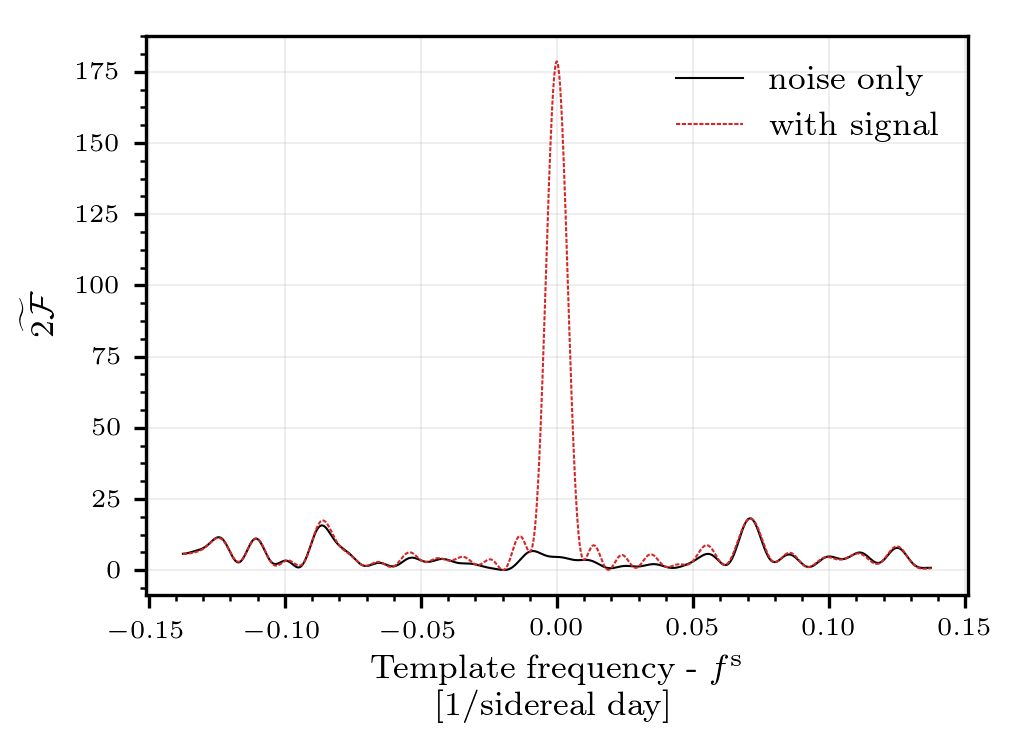
Figure 2: Numerically computed $\widetilde{2{\mathcal{F}}}$ for data (lasting 100 days) containing Gaussian noise only and the same data with an added simulated signal at frequency $f^{\mathrm{s}}$.

In addition to the $\mathrm{sinc}^{2}$ response for a signal, there are additional sideband peaks spaced at intervals of the inverse sidereal day; the presence of these can be deduced from Eq. (12) and (13) of Jaranowski et al. (1998), but for a detailed discussion see Sammut et al. (2014). To demonstrate this, in Fig. 3 we plot the $\widetilde{2{\mathcal{F}}}$ surface over the frequency for a signal lasting 5 days, such that the sideband spacing is approximately an order of magnitude larger than the signal width.

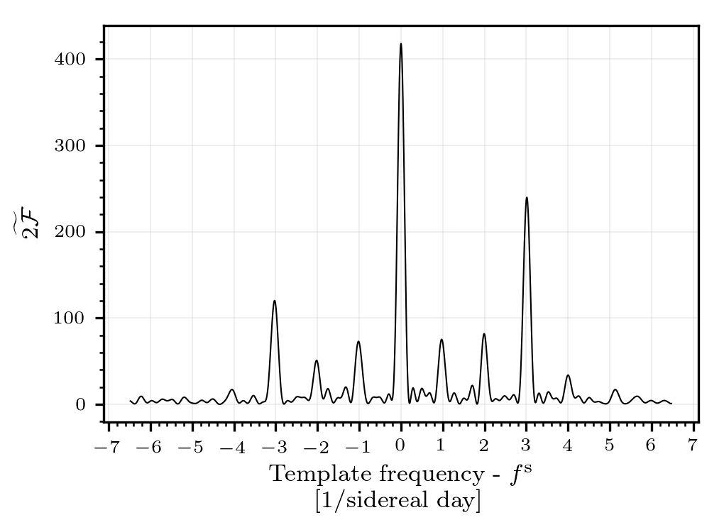
Figure 3: Numerically computed $\widetilde{2{\mathcal{F}}}$ for a simulated signal with frequency $f^{\mathrm{s}}$ in Gaussian noise lasting for $5$. Additionally, the signal was simulated with $\delta=0.50$ rad and $\cos(\iota)=0.10$.

Here, there are 9 peaks (8 of which are distinctive in this figure) spaced in intervals of the inverse sidereal day (the central peak being at the simulated signal frequency). The relative prominence of each side-peak varies strongly as a function of the declination in the sky and $\iota$, the angle between the spin-axis of the neutron star and the line of sight.

In Fig. 2 and 3, we have demonstrated that a signal in noise can have a complicated topology in the frequency space alone: having a main peak with associated $\mathrm{sinc}^{2}$ structure, sidebands, and other peaks due to Gaussian noise. In practice, we simultaneously search over other dimensions such as derivatives of the frequency and sky location which will also have a complicated structure with multiple peaks.

When running an MCMC simulation we must therefore be aware that in addition to the signal peak, the likelihood will contain multiple modes which may be either noise fluctuations, secondary peaks of the signal, or the signal peak itself. It is for these reasons that the parallel-tempered MCMC sampler (see Sec. II.2) is applied which can efficiently sample from such a multimodal posterior.

IV.4 Maximum size of prior parameter space

For a fixed sized search parameter space, any optimization routine, given finite resources, will fail if this space is too large. We quantify the size of a given space by $\mathcal{N}^{*}$, the approximate number of unit-mismatch templates. We now investigate the maximum $\mathcal{N}^{*}$ that this MCMC search can efficiently explore and explain what happens beyond this point.

An MCMC search is efficient if the walkers converge to the global maxima of the search space, an example can be seen in Fig. 1. On the other hand, if the search parameter space is too large compared to the size that the signal occupies, the walkers do not converge. Typically, this results in the walkers sampling the noisy background. In such cases, the search is, at best, an approximation of a random template bank (Messenger et al., 2009), but more often we find that the walkers end up getting stuck in multiple isolated maxima. As an example, in Fig. 4, we repeat the directed search shown in Fig. 1, but with a factor ${\color[rgb]{0,0,0}10^{3}}$ larger prior width in both $\Delta f$ and $\Delta\dot{f}$ such that the approximate number of templates is $\mathcal{N}^{*}\approx{\color[rgb]{0,0,0}10^{7}}$. Clearly, the MCMC search does not converge.

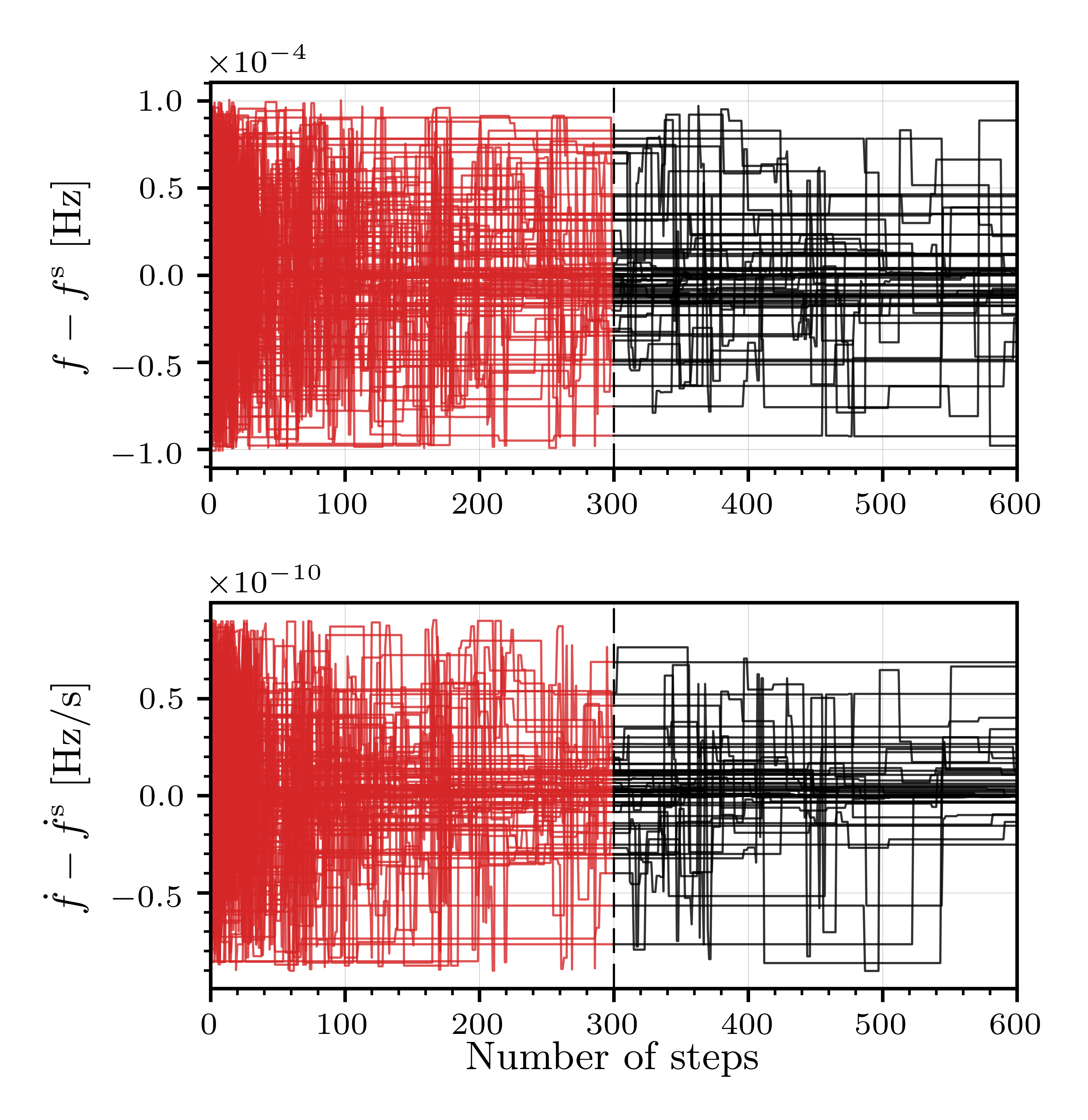
Figure 4: The progress of each walker in the MCMC simulation for a simulated signal in Gaussian noise, searching over a large directed search parameter space: the approximate number of unit-mismatch templates, defined in Section IV.2, is $\mathcal{N}^{*}\approx{\color[rgb]{0,0,0}10^{7}}$.

To quantify whether or not a simulation has converged, let us consider the resulting set of samples $\theta^{i}_{m}$, where $\theta\subseteq\boldsymbol{\mathbf{\lambda}}$, the upper index $i\in[1,N]$ labels the sample number, while the lower index $m\in[1,M]$ labels the walker number (recalling that we use an ensemble sampler). If we define the per-walker mean and variance as $\hat{\theta}_{m}$ and $\sigma_{m}^{2}$ and the mean over all walkers and steps to be $\hat{\theta}$, then the between-walker variance and the within-walker variance are given by

$$B_{\theta} \equiv\frac{N}{M-1}\sum_{m=1}^{M}(\hat{\theta}_{m}-\hat{\theta})^{2}$$ (26)

and

$$W_{\theta} \equiv\frac{1}{M}\sum_{m=1}^{M}(\hat{\theta}_{m})^{2}\,.$$ (27)

We can then define an intuitive way to quantify if the walkers have converged by calculating the ratio

$$\mathcal{Q}_{\theta} \equiv\frac{B_{\theta}}{W_{\theta}}\,.$$ (28)

for $\mathcal{Q}_{\theta}\gg 1$, the within-walker variance is much smaller than the variance between walkers, indicative that they are not converged, as in Fig. 4, while $\mathcal{Q}\sim 1$ indicates they have converged, as in Fig. 1.

This ratio is closely related to the Gelman-Rubin statistic (Gelman and Rubin, 1992; Brooks and Gelman, 1998) which was developed to monitor convergence of single-chain samplers by running multiple independent MCMC simulations. There are however theoretical issues in using the Gelman-Rubin statistic for ensemble samplers that go beyond the scope of this paper. For now, we find it is sufficient to use the intuitive ratio defined in Eq. (28) to assess safe values of $\mathcal{N}^{*}$. A possible alternative might be to use the ACT. However, to safely calculate this (using the methods defined in Vousden et al. (2016); Foreman-Mackey et al. (2013)), one needs to run the simulation until convergence. Since we want to investigate when (in a reasonable amount of computation time) the walkers do not converge, it is simpler to use $\mathcal{Q}_{\theta}$.

In a data set of 10 days, we simulate Gaussian noise and a signal with a sensitivity depth (defined in Eq. (19)) of $\mathcal{D}={\color[rgb]{0,0,0}40}$. Then, we perform a directed search (over $f$ and $\dot{f}$). The prior for the search is uniform in frequency and spin-down centered on the simulated signal and chosen such that the effective number of templates is $\mathcal{N}^{*}$.

Taking four different search setups (including the default setup used throughout this work, $N_{t}=3$ and 300 burn-in and production steps), we repeat the process 500 times in a Monte Carlo (MC) study. For each setup, we vary $\mathcal{N}^{*}$ and in Fig. 5 we plot the mean maximum of $\mathcal{Q}_{f}$ and $\mathcal{Q}_{\dot{f}}$. For the default setup, we also plot the individual results from the MC study to illustrate the variability about the mean.

This figure illustrates that using a greater number of temperatures and steps can improve the convergence efficiency. For the default setup, we conservatively define $\mathcal{N}^{*}_{\mathrm{max}}\equiv{\color[rgb]{0,0,0}1000}$ in order to ensure that the $\mathcal{Q}\sim 1$ such that the sampler will converge

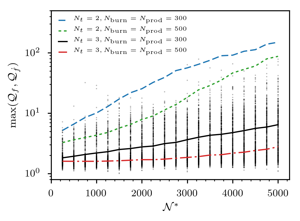
Figure 5: Study of how $\mathcal{Q}$ (defined in Eq. (28)) depends on the size of the prior parameter space (quantified in terms of $\mathcal{N}^{*}$) and the search setups. Four MC studies are shown as line plots of the mean value. In each of the four MC studies, we vary the number of steps and the number of temperatures (the same maximum temperature, see Section II.2, is used throughout). To illustrate the variance in a single MC study, markers show the individual MC results for $N_{t}=3$ and $N_{\mathrm{\rm burn}}=N_{\mathrm{\rm prod}}=300$, the default setup used in the rest of this work.

V Hierarchical multistage follow-up

Semi-coherent detection statistics trade candidate significance for computational cost to detect a candidate. To illustrate how, in Fig. 6, we compare the significance, expressed as a p-value, as a function of frequency for a fully coherent and two semi-coherent searches of a signal in Gaussian data. This demonstrates that while the maximum significance of the fully coherent search is the largest (in that its p-value is the smallest of the three), the semi-coherent searches have wider peaks. For a template bank search, using a semi-coherent detection statistic means that fewer templates are required to cover the search space.

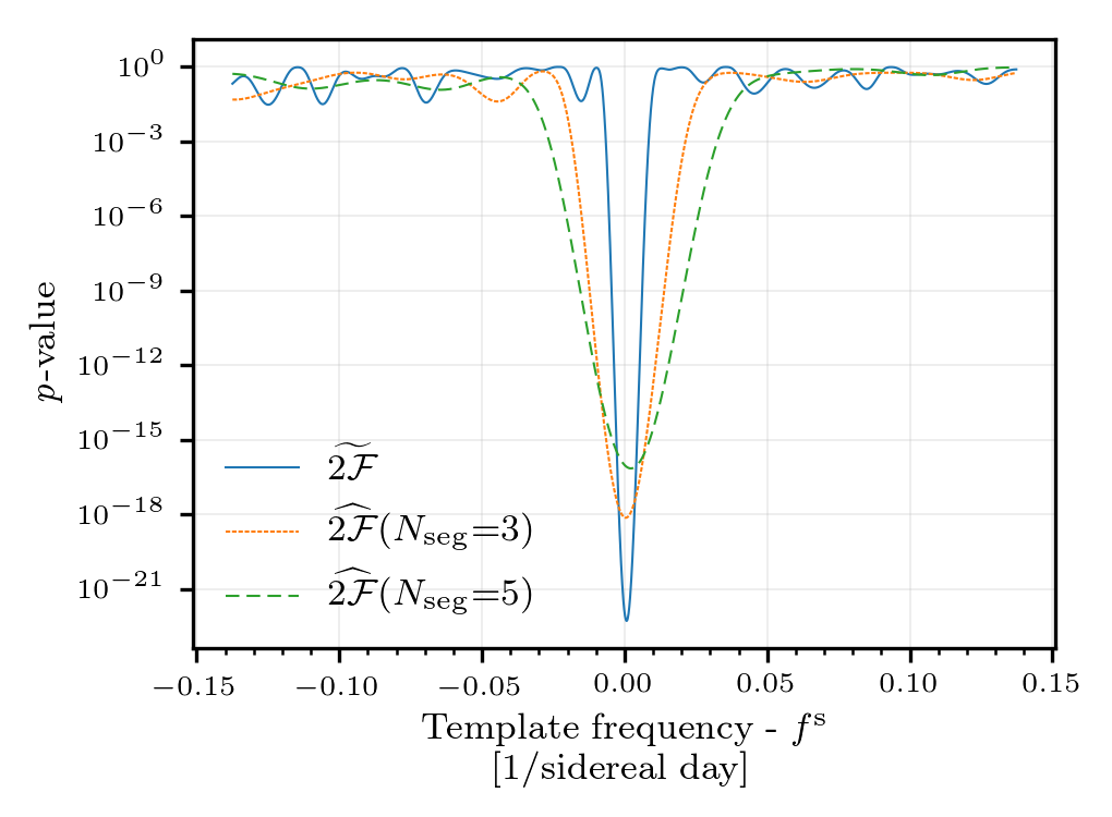
Figure 6: Comparison of the fully coherent $\widetilde{2\mathcal{F}}$ and semi-coherent $\widehat{2\mathcal{F}}$ as a function of the frequency for the same simulated signal in noise.

A semi-coherent search (e.g., an all-sky or directed search) may result in a list of promising candidates; these are then processed in a hierarchical follow-up in which the number of segments is decreased from $N_{\mathrm{\rm seg}}^{(0)}$, the number used in the initial search, to $N_{\mathrm{\rm seg}}^{(j_{\mathrm{max}})}{=}1$ (i.e., fully coherent). The ultimate aim of such a process is to either localize the candidate using a fully coherent detection statistic (i.e., calculate the maximum available significance) or refute the candidates as not being a standard CW if the detection statistic does not increase as expected.

The hierarchical follow-up can be done in two stages (cf. Brady and Creighton (2000)) with an initial semi-coherent stage followed directly by a fully coherent search. However, it was shown in a numerical study by Cutler et al. (2005) that a multi-stage hierarchical follow-up search using a decreasing ladder of segment numbers $\{N_{\mathrm{\rm seg}}^{(j)}\}$ can significantly improve the efficiency: ultimately they concluded that for template bank searches three semi-coherent stages provide the best trade-off between sensitivity and computational cost. For further examples of follow-up searches, see Shaltev and Prix (2013) which used a “Mesh Adaptive Direct Search” algorithm for optimization or Papa et al. (2016); Abbott et al. (2017d, e) for multi-stage gridded approaches.

In this work, we define a method to perform MCMC follow-up searches; we will make use of the idea that in a semi-coherent MCMC search, $N_{\mathrm{\rm seg}}$ can be thought of as a free parameter which adjusts the width of signal peaks (since the ${\mathcal{F}}$-statistic is proportional to our log-likelihood, cf. Eq. (18)).

The general principle is that, given a ladder of segment numbers, we run the MCMC sampler for each stage of the ladder, allowing enough time for the walkers to converge before moving to the next stage of the ladder. At each new stage, the previously converged walkers will now be overdispersed with respect to the new posterior distribution and will begin to converge, provided the change in the number of segments is sufficiently small so that they do not lose the signal. Repeating this process over the ladder of coherence times, at each stage the signal is better localized until the final fully coherent step. In the next Section, we define how to optimally choose the ladder of segment numbers.

It is worth noting that we do not test for convergence after each stage. Should the chains fail to converge, e.g., as in Fig. 4, then it is likely subsequent stages will remain unconverged. A potential future improvement is to implemented convergence checking, allowing stages to be curtailed if convergence is reached before some maximum allowed number of steps.

V.1 Optimal ladder of coherence times

Consider a candidate from a semi-coherent search at the $j$th stage with $N_{\mathrm{\rm seg}}^{(j)}$ segments and parameter uncertainty $\Delta\boldsymbol{\mathbf{\lambda}}^{(j)}$ (defined momentarily). The size of the signal within that uncertainty can be quantified by writing Eq. (23) with an explicit dependence on the number of segments and the parameter uncertainty,

$$\mathcal{N}^{*}\left(N_{\mathrm{\rm seg}}^{(j)},\Delta\boldsymbol{\mathbf{\lambda}}^{(j)}\right)=\sqrt{\mathrm{det}g\left(N_{\mathrm{\rm seg}}^{(j)}\right)}\;\mathrm{Vol}(\Delta\boldsymbol{\mathbf{\lambda}}^{(j)})\,.$$ (29)

For an MCMC search to be effective we need $\mathcal{N}^{*}(N_{\mathrm{\rm seg}}^{(j)},\Delta\boldsymbol{\mathbf{\lambda}}^{(j)})\lesssim\mathcal{N}^{*}_{\mathrm{max}}$ (see Section IV.4).

For the $j=0$ stage, the parameter uncertainty, $\Delta\boldsymbol{\mathbf{\lambda}}^{(0)}$, depends on the details of the initial search. However, if the initial search was too coarse for the MCMC method to be effective (i.e., $\Delta\boldsymbol{\mathbf{\lambda}}^{(0)}$ is too large), a template bank refinement can first be performed to reduce the uncertainty and ensure that $\mathcal{N}^{*}(N_{\mathrm{\rm seg}}^{(0)},\Delta\boldsymbol{\mathbf{\lambda}}^{(0)})\lesssim\mathcal{N}^{*}_{\mathrm{max}}$. If we then run the MCMC search using $N_{\mathrm{\rm seg}}=N_{\mathrm{\rm seg}}^{(0)}$ and a uniform prior based on $\Delta\boldsymbol{\mathbf{\lambda}}^{(0)}$, after convergence the walkers will be approximately bound in a posterior parameter space $\Delta\boldsymbol{\mathbf{\lambda}}^{(1)}\leq\Delta\boldsymbol{\mathbf{\lambda}}^{(0)}$. In a hierarchical search, one then proceeds to increase the coherence time to $N_{\mathrm{\rm seg}}^{(1)}<N_{\mathrm{\rm seg}}^{(0)}$ and again localize the signal. For our MCMC search, we similarly continue the MCMC simulation, but with fewer segments, better localizing the signal.

There are two consideration to be made in defining the ladder of coherence times. Firstly, the change in $N_{\mathrm{\rm seg}}$ between any two stages must be sufficiently small such that the walkers converge to the new posterior, formally this means that

$$\mathcal{N}^{*}(N_{\mathrm{\rm seg}}^{(j)},\Delta\boldsymbol{\mathbf{\lambda}}^{(j)})\leq\mathcal{N}^{*}_{\mathrm{max}}\,.$$ (30)

The second consideration is that we want to minimize the computational cost of the follow-up. This is achieved by choosing the maximal allowable decrease in $N_{\mathrm{\rm seg}}$ while still respecting Inequality (30).

The size of $\Delta\boldsymbol{\mathbf{\lambda}}^{(j+1)}$ is not known prior to running the $j$th stage of the search. However, since $\sqrt{g(N_{\mathrm{\rm seg}}^{(j)})}$ is the coordinate size a signal will occupy at a metric mismatch of one, (i.e., where the ${\mathcal{F}}$-statistic or log-likelihood is small compared to the peak value), it is conservative to assume that $\mathcal{N}^{*}(N_{\mathrm{\rm seg}}^{(j-1)},\Delta\boldsymbol{\mathbf{\lambda}}^{(j)})\approx 1$. Dividing this through Inequality (30) and taking the equality to minimize the computational cost, we see that one needs to find the largest $T_{\rm coh}^{(j)}$ which satisfies

$$\mathcal{N}^{*}_{\mathrm{max}}\approx\frac{\sqrt{g(T_{\rm coh}^{(j)})}}{\sqrt{g(T_{\rm coh}^{(j-1)})}}\,.$$ (31)

This can be done by increasing $T_{\rm coh}^{(j)}$ in steps until this criteria is satisfied; for efficiency, we instead define it as a minimization problem and use standard numerical solvers. Given an initial prior volume and coherence time, the optimal ladder of coherence times can then be precomputed saving computation time during the run (useful as the same setup can be applied to multiple candidates).

V.2 Example

We now provide an illustrative example of the follow-up method. We consider a directed search in 100 days of data from a single detector, with $\sqrt{S_{\rm n}}={\color[rgb]{0,0,0}1.0{\times}10^{-23}}$ Hz^-1/2 (at the fiducial frequency of the signal). The simulated signal has an amplitude $h_{0}=2.5{\times}10^{-25}$ such that the signal has a sensitivity depth of $\mathcal{D}=40.0$ Hz^-1/2 in the noise. We choose arbitrary phase-evolution parameters of $f^{\mathrm{s}}={\color[rgb]{0,0,0}30}$ Hz, $\dot{f}^{\mathrm{s}}={\color[rgb]{0,0,0}10^{-10}}$ Hz/s, and the sky location of the Crab pulsar. The initial prior uncertainty, $\Delta\boldsymbol{\mathbf{\lambda}}^{(0)}$, is $\Delta f={\color[rgb]{0,0,0}2.0{\times}10^{-5}}$ Hz and $\Delta\dot{f}={\color[rgb]{0,0,0}1.8{\times}10^{-11}}$ Hz/s. The optimal ladder of coherence times is precomputed using $\mathcal{N}^{*}_{\mathrm{max}}={\color[rgb]{0,0,0}1000}$ (i.e., the size of the fully coherent parameter space) and the resulting setup is given in Table 1.

Fig. 7 shows the progress of the MCMC sampler during the follow-up. For illustrative purposes, in this example we use ${\color[rgb]{0,0,0}100}$ steps per-stage, rather that the default $300$ as suggested in Section III.3. As expected from Table 1, during stage 0 the signal peak is broad with respect to the size of the prior volume, therefore the MCMC simulation quickly converges to it. At each subsequent stage, when the number of segments is reduced, the peak narrows and the samplers similarly converge to this new solution.

Table 1: The search setup used in Fig. 7, generated with $\mathcal{N}^{*}_{\mathrm{max}}={\color[rgb]{0,0,0}1000}$. The final column provides the approximate number of unit-mismatch templates at each stage calculated over the prior volume.

Stage	$N_{\mathrm{seg}}$	$T_{\mathrm{coh}}^{\rm days}$	$\mathcal{N}^{*}(N_{\mathrm{\rm seg}}^{(\ell)},\Delta\boldsymbol{\lambda}^{(0)})$
0	100	1.0	2.2
1	35	2.9	18.0
2	5	20.0	$8.8{\times}10^{2}$
3	1	100.0	$1.0{\times}10^{4}$

Figure 7: We show the progress of the 100 parallel walkers (see Fig. 1 for a description) during the MCMC simulation for the directed search parameters. Each vertical dashed line indicates the start of a new stage of the search (numbered on the top axis), the details of all stages are listed in Table 1.

V.3 Monte Carlo studies

In order to quantify how well the MCMC follow-up method works, we test its ability to successfully identify simulated signals in Gaussian noise. This will be done in a Monte Carlo (MC) study, with independent random realizations of the Gaussian noise. Such a method is analogous to the studies performed in Shaltev and Prix (2013), except that we present results as a function of the injected sensitivity depth, rather than the squared-SNR.

In Section V.3.1 and V.3.2, we perform MC studies for the follow-up of directed and all-sky searches. For both studies, we simulate an isotropic distribution of source orientations by drawing the amplitude parameters for each signal uniformly from $\phi\in[0,2\pi]$, $\psi\in[-\pi/4,\pi/4]$, and $\cos\iota\in[-1,1]$. However, we do not draw $h_{0}$ randomly, but run the MC study at a range of selected $h_{0}$ values to show how the MCMC follow-up performs as a function of sensitivity depth (we fix $\sqrt{S_{n}}={\color[rgb]{0,0,0}1\times 10^{-23}}$). The selection of phase-evolution parameters is discussed separately for each study.

The success of an MCMC follow-up search is evaluated by the maximum $\widetilde{2{\mathcal{F}}}$ value found in the final, fully coherent stage of the search. We begin each MC study by first estimating a background distribution for the maximum $\widetilde{2{\mathcal{F}}}$ value found in noise and using this to define a threshold value $\widetilde{2{\mathcal{F}}}_{\rm th}$; for the simulated signals in noise we then ascribe results with a maximum $\widetilde{2{\mathcal{F}}}$ above this threshold as “recovered” whilst those falling short are not recovered.

The hierarchical multi-stage MCMC search may fail to detect a candidate for two distinct reasons: (i) the simulated signal is not sufficiently loud with respect to the background noise to be detected and (ii) the simulated signal is sufficiently loud, but the MCMC fails to recover it. The first reason can be understood as saying that, even for a template bank search which covers the search space with infinite resolution, for sufficiently weak signals, the proportion of recovered candidates tends to zero. More precisely this behavior is the expected theoretical optimal performance detection probability for an infinitely dense fully coherent search of data containing isotropically-distributed signals as calculated by Wette (2012). In this study, we want to understand how the MCMC follow-up performs with respect to reason (ii). Therefore, we will plot the recovered fraction (in the MC study) as a function of the sensitivity depth, and compare this against the theoretical optimal performance (i.e., using Eq. (3.8) of Wette (2012) to relate the averaged-SNR to the sensitivity depth). Deviations of the MC study with respect to the theoretical optimal performance indicate any weakness in the MCMC follow-up method itself.

V.3.1 Follow-up of candidates from a directed search

For the directed MC study, we simulate signals following the example described in Sec. V.2, except that the simulated frequency and spin-down are selected randomly from the inner half of the initial prior uncertainty. As in the example, the prior is defined to be uniform over the full uncertainty box and the duration is 100 days. Therefore, the optimal setup is also the same and given in Table 1. Each stage is run for 300 steps before moving to the next stage of the ladder, after the final stage an additional 300 production steps are taken.

Characterizing the search in Gaussian noise without a signal first, we simulate ${\color[rgb]{0,0,0}1\times 10^{3}}$ realizations and perform the follow-up search on these. The largest observed value was found to be ${\color[rgb]{0,0,0}50.9}$. From this, we can set an arbitrary threshold for the detection statistic of $\widetilde{2{\mathcal{F}}}_{\rm th}={\color[rgb]{0,0,0}60}$.

Running 500 MC simulations of Gaussian noise with a simulated signal, in Fig. 8 we plot the fraction of the MC simulations which where recovered (i.e., $\widetilde{2{\mathcal{F}}}^{\rm max}>\widetilde{2{\mathcal{F}}}_{\rm th}={\color[rgb]{0,0,0}60}$) and compare this against the theoretical optimal performance as discussed earlier, given the threshold. The figure demonstrates that the recovery power of the MCMC follow-up shows negligible losses compared to the theoretical optimal performance.

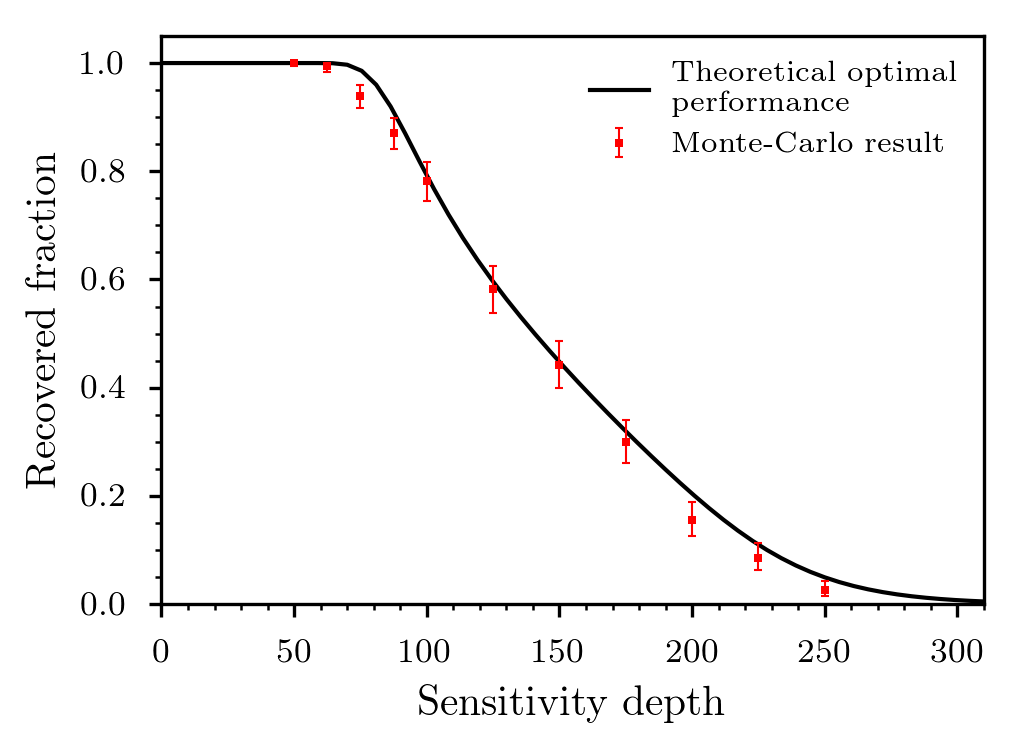
Figure 8: Recovery fraction for the directed follow-up. The MC results come from random draws searches using the setup described in Table 1.

V.3.2 Follow-up of candidates from an all-sky search

We now test the follow-up method when applied to candidates from an all-sky search which, by definition, have uncertain sky-position parameters $\alpha$ and $\delta$. Searching over these parameters, in addition to the frequency and spin-down not only increases the parameter space volume that needs to be searched, but also adds difficulty due to correlations between the sky-position and spin-down.

To replicate the condition of candidates from an all-sky search, we draw the candidate positions isotropically from the unit sphere (i.e., $\alpha$ uniform on $[0,2\pi]$ and $\delta=\sin^{-1}(u)$ where $u$ is uniform on $[-1,1]$). We then place an uncertainty box containing the candidates with a width $\Delta\alpha=\Delta\delta={\color[rgb]{0,0,0}0.05}$; this box is chosen in such a way that the location of the candidate has a uniform probability distribution within the box. This neglects the non-uniform variation in $\delta$ over the sky-patch, but, given the small size of the sky-patch, should not cause any significant bias. The frequency, spin-down, and amplitude parameters are chosen in the same way as for the directed search (Section V.3.1). The optimal setup is precomputed for this prior and given in Table 2. Each stage is run for 300 steps before moving to the next stage of the ladder, after the final stage an additional 300 production steps are taken.

Table 2: Run-setup for the all-sky follow-up MC study, generated with $\mathcal{N}^{*}_{\mathrm{max}}=1000$. The approximate number of unit-mismatch templates over the initial search space was computed at the equator (i.e., $\delta=0$) which produces the largest volumes.

Stage	$N_{\mathrm{seg}}$	$T_{\mathrm{coh}}^{\rm days}$	$\mathcal{N}^{*}(N_{\mathrm{\rm seg}}^{(\ell)},\Delta\boldsymbol{\lambda}^{(0)})$
0	100	1.0	8.4
1	35	2.9	$5.6{\times}10^{2}$
2	6	16.7	$5.2{\times}10^{5}$
3	1	100.0	$2.5{\times}10^{7}$

Again, we first characterize the behavior of the all-sky follow-up by applying it to ${\color[rgb]{0,0,0}1\times 10^{3}}$ realizations of Gaussian noise. The largest $\widetilde{2{\mathcal{F}}}$ value was found to be ${\color[rgb]{0,0,0}58.4}$. This is larger than the value found for the directed search, although both use the same number of Gaussian noise trials, and therefore must result from an increased number of independent templates. As a result we correspondingly increase our arbitrary detection threshold for the all-sky search to $\widetilde{2{\mathcal{F}}}_{\rm tr}={\color[rgb]{0,0,0}70}$.

Running 500 MC simulations of Gaussian noise with randomly drawn signals, the resulting recovery fraction as a function of the injected sensitivity depth is given in Fig. 9. We find that the all-sky Monte Carlo has a detection efficiency close to the theoretical optimal performance.

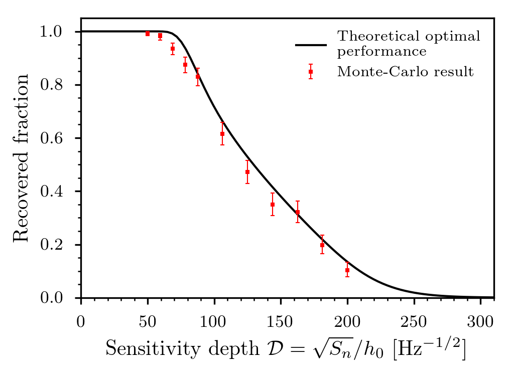
Figure 9: Recovery fraction for the all-sky follow-up. The MC results come from random draws searches using the setup described in Table 2.

VI Computation time estimates

In this section, we will provide an approximate timing model for the MCMC search method implemented in pyfstat.

The computation time of an MCMC search can be split into two contributions, the evaluation of the ${\mathcal{F}}$-statistic and all other operations, which we refer to as the pyfstat-overhead (i.e., computing the prior probabilities, generating the proposal jumps, evaluating the jumps and other minor contributions).

Timing the evaluation of the “Demod” ${\mathcal{F}}$-statistic (used in this analysis) is discussed in Prix (2017). The time to compute a single-$\boldsymbol{\mathbf{\lambda}}$ template for a single detector can be written as $\tau_{\mathcal{F}}^{\mathrm{eff}}=N_{\mathrm{SFT}}\tau_{\mathrm{LD}}$, where $N_{\mathrm{SFT}}$ is the number of short Fourier transforms (SFTs) (the core data product used in CW searches), which will depend on the data duration and SFT length (typically 1800 s). We can further decompose $\tau_{\mathrm{LD}}$ as

$$\tau_{\mathrm{LD}}=\tau^{(0)}_{\mathrm{core,LD}}+b\tau^{(0)}_{\mathrm{buffer,LD}}\,,$$ (32)

where $\tau^{(0)}_{\mathrm{core,LD}}$ is the core time to compute a single ${\mathcal{F}}$-statistic evaluation (excluding the time to compute any buffered quantities), $\tau^{(0)}_{\mathrm{buffer,LD}}$ is the time to compute the buffered quantities, and $b\in[0,1]$ the “buffer miss fraction” quantifies how often the buffer needs to be recomputed between evaluations Prix (2017). For our purposes, it is sufficient to note that for all-sky searches $b=1$ (if the sky position changes between steps), but for directed searches $b\approx 1$.

The pyfstat-overhead will depend on whether the search is fully or semi-coherent. We now discuss each of these in turn.

VI.1 Fully coherent timing model

For any fully coherent search using the pyfstat code, the time per-call is given by

$$\tau_{\mathrm{FC}}=(\tau^{(0)}_{\mathrm{S}}+\tau_{\mathrm{LD}}N_{\mathrm{SFT}})\,,$$ (33)

such that the total time for a fully coherent MCMC search with $N_{w}$ walkers and $N_{t}$ temperatures is

$$\mathcal{T}_{\mathrm{FC}}^{\mathrm{MCMC}}=\tau_{\mathrm{FC}}(N_{\mathrm{\rm burn}}+N_{\mathrm{\rm prod}})N_{w}N_{t}\,.$$ (34)

Note that this timing model is independent of the state of the MCMC sampler, i.e., whether or not it has converged to a single peak.

To estimate these timing coefficients, we run MC studies of MCMC searches for various data spans ranging from 25 days to 100 days. Profiling the run times, we estimate $\tau_{\mathrm{LD}}$ from the calls to XLALComputeFstat(), then $\tau^{(0)}_{\mathrm{S}}$ as the remaining run time. The resulting estimates are given in Table 3.

Table 3: Estimates of the fundamental timing coefficients made on a Lenovo T460p with an Intel(R) Core(TM) i5-6300HQ CPU @ 2.30GHz.

		$\tau_{\mathrm{LD}}$ [s]	$\tau^{(0)}_{\mathrm{T}}$ [s]	$\tau^{(0)}_{\mathrm{S}}$	$\tau^{(0)}_{\mathrm{C}}$ [s]
Directed	fully coherent	$7.4\times 10^{-8}\pm 27\%$	—	$6.4\times 10^{-5}\pm 14\%$	—
	semi-coherent	$1.3\times 10^{-7}\pm 35\%$	$1.5\times 10^{-8}\pm 6\%$	$9.1\times 10^{-5}\pm 23\%$	$5.5\times 10^{-6}\pm 14\%$
All-sky	fully coherent	$5.0\times 10^{-7}\pm 14\%$	—	$1.0\times 10^{-4}\pm 19\%$	—
	semi-coherent	$5.2\times 10^{-7}\pm 18\%$	$1.5\times 10^{-8}\pm 6\%$	$1.2\times 10^{-4}\pm 25\%$	$5.8\times 10^{-6}\pm 19\%$

The estimated $\tau_{\mathrm{LD}}$ differs between the all-sky and directed searches since $b=1$ in the former, but $0$ for the latter. The estimated values of $\tau_{\mathrm{LD}}$ are in agreement with values found using gridded searches on the same machine, and the values found in Prix (2017). From this table, we see that the evaluation of the ${\mathcal{F}}$-statistic will dominate the timing when $N_{\mathrm{SFT}}\gtrsim 900$ $(200)$, which for 1800 s SFTs corresponds to $\sim 18$ $(4)$ days for the directed (all-sky) search.

The dominant factor required to determine the cost of a run is the number of steps (typically one uses a few hundred walkers and two or three temperatures). The number of steps depends on the ACT. For the directed MC study we found the largest ACT to be $\sim 15$. To safely account for burn-in we therefore suggest the total number of steps be $\sim 20\times 15=300$. Meanwhile, for the all-sky MC study we found the largest ACT to be $\sim 90$, so an all-sky search requires a factor of $6$ more steps. These numbers are approximate and will depend on the other search setup parameters (i.e., using only a single temperature will require a larger numbers of steps); a MC simulation could be run prior to a follow-up to tune $N_{w},N_{t}$, and the number of required burn-in and production steps.

VI.2 Semi-coherent timing model

The current implementation of pyfstat implements a semi-coherent search by using the ComputeTransientFstatMap() functions of LALSUITE. This is done to avoid repeated computation of intermediate data products, but itself incurs additional computational cost proportional to the number of segments. We can model this by introducing a new timing coefficient $\tau^{(0)}_{\mathrm{T}}$ such that the semi-coherent timing per-call is

$$\begin{split}\tau_{\mathrm{SC}}&=\left[\tau^{(0)}_{\mathrm{S}}+\tau^{(0)}_{\mathrm{C}}N_{\mathrm{\rm seg}}+\left(\tau_{\mathrm{LD}}+\tau^{(0)}_{\mathrm{T}}N_{\mathrm{\rm seg}}\right)N_{\mathrm{SFT}}\right]\,,\end{split}$$ (35)

with the total time being

$$\tau^{\mathrm{MCMC}}_{\mathrm{SC}}=\tau_{\mathrm{SC}}(N_{\mathrm{\rm burn}}+N_{\mathrm{\rm prod}})N_{w}N_{t}\,.$$ (36)

Again running a MC study, we present estimates of these timing constants in Table 3.

VI.3 Follow-up timing model

The computing cost for a given follow-up run setup can be estimated by summing the cost for each stage using Eq. (34) and (36). As an example, the directed search run setup given in Table 1 has an estimated run time of $\sim{\color[rgb]{0,0,0}432}$ s while the all-sky run setup in Table 2 has an estimated run time of $\sim{\color[rgb]{0,0,0}2200}$ s. The limitation of this method is that it requires the candidate to be sufficiently well localized at the coherence time of the original search. Therefore, an additional refinement stage may be required prior to the MCMC follow-up which will add an additional overhead.

VII Conclusion

We investigate the use of an MCMC method in continuous-gravitational-wave searches. Compared to template-bank searches, these enable efficient exploration of the parameter space and posterior parameter inference. However, these advantages may only be reaped when the signal occupies a reasonably large fraction of the prior volume. We quantify this through $\mathcal{N}^{*}$, the approximate number of unit-mismatch templates required to cover the prior volume. In particular, the prior volume must be sufficiently small in the sense that $\mathcal{N}^{*}\lesssim\mathcal{N}^{*}_{\mathrm{max}}$. For this reason, MCMC methods are generally not suitable as an initial search method in wide parameter spaces where this condition is not met.

We have investigated $\mathcal{N}^{*}_{\mathrm{max}}$ for the ptemcee sampler with a particular setup (see Sec. II.2) and fixed number of steps, and found $\mathcal{N}^{*}_{\mathrm{max}}\sim 1000$ to be a reasonably safe choice. In general, this value will depend on the sampler, setup, and number of steps. However, we expect our general conclusion to hold for different samplers (including nested sampling methods), but $\mathcal{N}^{*}_{\mathrm{max}}$ could differ. In the future we hope to extend this work to use a variety of samplers, in which case $\mathcal{N}^{*}_{\mathrm{max}}$ will provide a method to compare their efficiency.

We furthermore propose an MCMC-based hierarchical multi-stage follow-up for signal candidates found in semi-coherent wide-parameter-space searches. The MCMC methods are again found to be suitable in this context. We define a method to determine the optimal setup, balancing computational efficiency against robustness to losing signals. Testing against the theoretical optimal performance (i.e., an infinitely fine template bank), we find that the loss of signals inherently due to the MCMC procedure is small.

VIII Acknowledgments

We thank David Keitel, Simone Mastrogiovanni, Grant Meadors, and Karl Wette for useful comments during the development of this work.

References

- Aasi et al. (2015) J. Aasi et al. (LIGO Scientific Collaboration), “Advanced LIGO,” Class. Quantum Grav. 32, 074001 (2015), arXiv:1411.4547 [gr-qc] .
- Acernese et al. (2015) F. Acernese et al. (Virgo Collaboration), “Advanced Virgo: a second-generation interferometric gravitational wave detector,” Class. Quantum Grav. 32, 024001 (2015), arXiv:1408.3978 [gr-qc] .
- Abbott et al. (2017a) B. P. Abbott et al. (LIGO Scientific Collaboration and Virgo Collaboration), “First Search for Gravitational Waves from Known Pulsars with Advanced LIGO,” Astrophys. J. 839, 12 (2017a).
- Abbott et al. (2017b) B. P. Abbott et al. (LIGO Scientific Collaboration and Virgo Collaboration), “Search for gravitational waves from Scorpius X-1 in the first Advanced LIGO observing run with a hidden Markov model,” Phys. Rev. D 95, 122003 (2017b).
- Abbott et al. (2017c) B. P. Abbott et al. (LIGO Scientific Collaboration and Virgo Collaboration), “Upper Limits on Gravitational Waves from Scorpius X-1 from a Model-based Cross-correlation Search in Advanced LIGO Data,” Astrophys. J. 847, 47 (2017c), arXiv:1706.03119 [astro-ph.HE] .
- Abbott et al. (2017d) B. P. Abbott et al. (LIGO Scientific Collaboration and Virgo Collaboration), “All-sky search for periodic gravitational waves in the O1 LIGO data,” Phys. Rev. D 96, 062002 (2017d), arXiv:0708.3818 [gr-qc] .
- Abbott et al. (2017e) B. P. Abbott et al. (LIGO Scientific Collaboration and Virgo Collaboration), “First low-frequency Einstein@Home all-sky search for continuous gravitational waves in Advanced LIGO data,” Phys. Rev. D 96, 122004 (2017e).
- Abbott et al. (2017) B. P. Abbott et al. (The LIGO Scientific Collaboration and the Virgo Collaboration), “First narrow-band search for continuous gravitational waves from known pulsars in advanced detector data,” Phys. Rev. D 96, 122006 (2017).
- Jaranowski et al. (1998) P. Jaranowski, A. Królak, and B. F. Schutz, “Data analysis of gravitational-wave signals from spinning neutron stars: The signal and its detection,” Phys. Rev. D 58, 063001 (1998), gr-qc/9804014 .
- Prix (2009) R. Prix, “Gravitational Waves from Spinning Neutron Stars,” in Astrophysics and Space Science Library, Astrophysics and Space Science Library, Vol. 357, edited by W. Becker (2009) p. 651, https://dcc.ligo.org/LIGO-P060039/public.
- Brady et al. (1998) P. R. Brady et al., “Searching for periodic sources with LIGO,” Phys. Rev. D 57, 2101–2116 (1998), gr-qc/9702050 .
- Prix and Shaltev (2012) R. Prix and M. Shaltev, “Search for continuous gravitational waves: Optimal StackSlide method at fixed computing cost,” Phys. Rev. D 85, 084010 (2012), arXiv:1201.4321 [gr-qc] .
- Brady and Creighton (2000) P. R. Brady and T. Creighton, “Searching for periodic sources with LIGO. II. Hierarchical searches,” Phys. Rev. D 61, 082001 (2000), gr-qc/9812014 .
- Krishnan et al. (2004) B. Krishnan et al., “Hough transform search for continuous gravitational waves,” Phys. Rev. D 70, 082001 (2004), gr-qc/0407001 .
- Astone et al. (2014) P. Astone, A. Colla, S. D’Antonio, S. Frasca, and C. Palomba, “Method for all-sky searches of continuous gravitational wave signals using the frequency-Hough transform,” Phys. Rev. D 90, 042002 (2014), arXiv:1407.8333 [astro-ph.IM] .
- Abbott et al. (2008) B. P. Abbott et al. (LIGO Scientific Collaboration and Virgo Collaboration), “All-sky search for periodic gravitational waves in LIGO S4 data,” Phys. Rev. D 77, 022001 (2008), arXiv:0708.3818 [gr-qc] .
- Pletsch and Allen (2009) H. J. Pletsch and B. Allen, “Exploiting Large-Scale Correlations to Detect Continuous Gravitational Waves,” Phys. Rev. Lett. 103, 181102 (2009), arXiv:0906.0023 [gr-qc] .
- Pletsch (2008) H. J. Pletsch, “Parameter-space correlations of the optimal statistic for continuous gravitational-wave detection,” Phys. Rev. D 78, 102005 (2008), arXiv:0807.1324 [gr-qc] .
- Christensen and Meyer (1998) N. Christensen and R. Meyer, “Markov chain monte carlo methods for bayesian gravitational radiation data analysis,” Phys. Rev. D 58, 082001 (1998).
- Christensen and Meyer (2001) N. Christensen and R. Meyer, “Using markov chain monte carlo methods for estimating parameters with gravitational radiation data,” Phys. Rev. D 64, 022001 (2001).
- Christensen et al. (2004a) N. Christensen, R. Meyer, and A. Libson, “A Metropolis Hastings routine for estimating parameters from compact binary inspiral events with laser interferometric gravitational radiation data,” Class. Quantum Grav. 21, 317–330 (2004a).
- Röver et al. (2006) C. Röver, R. Meyer, and N. Christensen, “Bayesian inference on compact binary inspiral gravitational radiation signals in interferometric data,” Class. Quantum Grav. 23, 4895–4906 (2006), gr-qc/0602067 .
- Veitch et al. (2015) J. Veitch et al., “Parameter estimation for compact binaries with ground-based gravitational-wave observations using the LALInference software library,” Phys. Rev. D 91, 042003 (2015), arXiv:1409.7215 [gr-qc] .
- Christensen et al. (2004b) N. Christensen, R. J. Dupuis, G. Woan, et al., “Metropolis-Hastings algorithm for extracting periodic gravitational wave signals from laser interferometric detector data,” Phys. Rev. D 70, 022001 (2004b), gr-qc/0402038 .
- Umstätter et al. (2004) R. Umstätter et al., “Estimating the parameters of gravitational waves from neutron stars using an adaptive MCMC method,” Class. Quantum Grav. 21, S1655–S1665 (2004).
- Veitch (2007) J. D. Veitch, Applications of Markov Chain Monte Carlo methods to continuous gravitational wave data analysis, Ph.D. thesis, University of Glasgow (2007).
- Abbott et al. (2010) B. P. Abbott et al. (The LIGO Scientific Collaboration and the Virgo Collaboration), “Searches for Gravitational Waves from Known Pulsars with Science Run 5 LIGO Data,” Astrophys. J. 713, 671–685 (2010), arXiv:0909.3583 [astro-ph.HE] .
- Pitkin et al. (2012) M. Pitkin et al., “A new code for parameter estimation in searches for gravitational waves from known pulsars,” in Journal of Physics Conference Series, Vol. 363 (2012) p. 012041, arXiv:1203.2856 [astro-ph.HE] .
- Pitkin et al. (2017) M. Pitkin et al., “A nested sampling code for targeted searches for continuous gravitational waves from pulsars,” ArXiv e-prints (2017), arXiv:1705.08978 [gr-qc] .
- Umstätter (2006) R. Umstätter, Bayesian strategies for gravitational radiation data analysis, Ph.D. thesis, The University of Auckland (2006).
- Ashton (2017) G. Ashton, “PyFstat-v1.1.0,” (2017), 10.5281/zenodo.1069408.
- MacKay (2003) David J. C. MacKay, Information Theory, Inference and Learning Algorithms (Cambridge University Press, 2003).
- Gelman et al. (2013) A. Gelman et al., Bayesian Data Analysis, 3rd ed. (CRC Press, 2013).
- Vousden et al. (2016) W. D. Vousden, W. M. Farr, and I. Mandel, “Dynamic temperature selection for parallel tempering in markov chain monte carlo simulations,” Mon. Notices Royal Astron. Soc. 455, 1919–1937 (2016).
- Foreman-Mackey et al. (2013) D. Foreman-Mackey, D. W. Hogg, D. Lang, and J. Goodman, “emcee: The MCMC Hammer,” Publications of the Astronomical Society of Pacific 125, 306–312 (2013), arXiv:1202.3665 [astro-ph.IM] .
- Goodman and Weare (2010) J. Goodman and J. Weare, “Ensemble samplers with affine invariance,” Communications in Applied Mathematics and Computational Science, Vol. 5, No. 1, p. 65-80, 2010 5, 65–80 (2010).
- Swendsen and Wang (1986) R. H. Swendsen and J.-S. Wang, “Replica Monte Carlo Simulation of Spin-Glasses,” Phys. Rev. Lett. 57, 2607–2609 (1986).
- Sokal (1997) A. Sokal, “Monte carlo methods in statistical mechanics: foundations and new algorithms,” in Functional integration, Vol. 361, edited by Folacci A. DeWitt-Morette C., Cartier P. (Springer, Boston, MA, 1997) pp. 131–192.
- Akeret et al. (2013) J. Akeret, S. Seehars, A. Amara, A. Refregier, and A. Csillaghy, “CosmoHammer: Cosmological parameter estimation with the MCMC Hammer,” Astronomy and Computing 2, 27 – 39 (2013), arXiv:1212.1721 [astro-ph.CO] .
- Allison and Dunkley (2014) R. Allison and J. Dunkley, “Comparison of sampling techniques for Bayesian parameter estimation,” Mon. Notices Royal Astron. Soc. 437, 3918–3928 (2014), arXiv:1308.2675 [astro-ph.IM] .
- Raftery and Lewis (1991) Adrian E Raftery and Steven Lewis, How many iterations in the Gibbs sampler?, Tech. Rep. (Washing State University, Department of Statistics, 1991).
- Cowles and Carlin (1996) M. K. Cowles and B. P. Carlin, “Markov chain monte carlo convergence diagnostics: A comparative review,” Journal of the American Statistical Association 91, 883–904 (1996).
- Hogg and Foreman-Mackey (2017) David W Hogg and Daniel Foreman-Mackey, “Data analysis recipes: Using markov chain monte carlo,” arXiv preprint arXiv:1710.06068 (2017).
- Prix and Krishnan (2009) R. Prix and B. Krishnan, “Targeted search for continuous gravitational waves: Bayesian versus maximum-likelihood statistics,” Class. Quantum Grav. 26, 204013 (2009), arXiv:0907.2569 [gr-qc] .
- Cutler and Schutz (2005) C. Cutler and B. F. Schutz, “Generalized F-statistic: Multiple detectors and multiple gravitational wave pulsars,” Phys. Rev. D 72, 063006 (2005), gr-qc/0504011 .
- Whelan et al. (2014) John T. Whelan, Reinhard Prix, Curt J. Cutler, and Joshua L. Willis, “New coordinates for the amplitude parameter space of continuous gravitational waves,” Classical and Quantum Gravity 31, 065002 (2014).
- Prix et al. (2011) R. Prix, S. Giampanis, and C. Messenger, “Search method for long-duration gravitational-wave transients from neutron stars,” Phys. Rev. D 84, 023007 (2011), arXiv:1104.1704 [gr-qc] .
- LIGO Scientific Collaboration (2014) LIGO Scientific Collaboration, “LALSuite: FreeSoftware (GPL) Tools for Data-Analysis,” (2014), https://www.lsc-group.phys.uwm.edu/daswg/projects/lalsuite.html.
- Pletsch (2010) H. J. Pletsch, “Parameter-space metric of semicoherent searches for continuous gravitational waves,” Phys. Rev. D 82 (2010), 10.1103/PhysRevD.82.042002, arXiv:1005.0395 .
- Wette and Prix (2013) K. Wette and R. Prix, “Flat parameter-space metric for all-sky searches for gravitational-wave pulsars,” Phys. Rev. D 88, 123005 (2013), arXiv:1310.5587 [gr-qc] .
- Wette (2015) K. Wette, “Parameter-space metric for all-sky semicoherent searches for gravitational-wave pulsars,” Phys. Rev. D 92, 082003 (2015), arXiv:1508.02372 [gr-qc] .
- Owen (1996) B. J. Owen, “Search templates for gravitational waves from inspiraling binaries: Choice of template spacing,” Phys. Rev. D 53, 6749–6761 (1996), gr-qc/9511032 .
- Balasubramanian et al. (1996) R. Balasubramanian, B. S. Sathyaprakash, and S. V. Dhurandhar, “Gravitational waves from coalescing binaries: Detection strategies and Monte Carlo estimation of parameters,” Phys. Rev. D 53, 3033–3055 (1996), gr-qc/9508011 .
- Prix (2007) R. Prix, “Template-based searches for gravitational waves: efficient lattice covering of flat parameter spaces,” Class. Quantum Grav. 24, S481–S490 (2007), arXiv:0707.0428 [gr-qc] .
- Messenger et al. (2009) C. Messenger, R. Prix, and M. A. Papa, “Random template banks and relaxed lattice coverings,” Phys. Rev. D 79, 104017 (2009), arXiv:0809.5223 [gr-qc] .
- Owen and Sathyaprakash (1999) B. J. Owen and B. S. Sathyaprakash, “Matched filtering of gravitational waves from inspiraling compact binaries: Computational cost and template placement,” Phys. Rev. D 60, 022002 (1999), gr-qc/9808076 .
- Cutler et al. (2005) C. Cutler, I. Gholami, and B. Krishnan, “Improved stack-slide searches for gravitational-wave pulsars,” Phys. Rev. D 72, 042004 (2005), gr-qc/0505082 .
- Prix and Itoh (2005) R. Prix and Y. Itoh, “Global parameter-space correlations of coherent searches for continuous gravitational waves,” Class. Quantum Grav. 22, 1003 (2005), gr-qc/0504006 .
- Sammut et al. (2014) L. Sammut, C. Messenger, A. Melatos, and B. J. Owen, “Implementation of the frequency-modulated sideband search method for gravitational waves from low mass x-ray binaries,” Phys. Rev. D 89, 043001 (2014), arXiv:1311.1379 [gr-qc] .
- Gelman and Rubin (1992) A. Gelman and D. B. Rubin, “Inference from Iterative Simulation Using Multiple Sequences,” Statistical Science 7, 457–472 (1992).
- Brooks and Gelman (1998) S. P. Brooks and A. Gelman, “General methods for monitoring convergence of iterative simulations,” Journal of Computational and Graphical Statistics 7, 434–455 (1998).
- Shaltev and Prix (2013) M. Shaltev and R. Prix, “Fully coherent follow-up of continuous gravitational-wave candidates,” Phys. Rev. D 87, 084057 (2013), arXiv:1303.2471 [gr-qc] .
- Papa et al. (2016) M. A. Papa et al., “Hierarchical follow-up of subthreshold candidates of an all-sky einstein@home search for continuous gravitational waves on ligo sixth science run data,” Phys. Rev. D 94, 122006 (2016).
- Wette (2012) K. Wette, “Estimating the sensitivity of wide-parameter-space searches for gravitational-wave pulsars,” Phys. Rev. D 85, 042003 (2012), arXiv:1111.5650 [gr-qc] .
- Prix (2017) R. Prix, “Characterizing timing and memory-requirements of the F-statistic implementations in LALSuite,” (2017), https://dcc.ligo.org/LIGO-T1600531/public.