Improving the Decoding Threshold of Tailbiting Spatially Coupled LDPC Codes by Energy Shaping

Abstract

We show how the iterative decoding threshold of tailbiting spatially coupled (SC) low-density parity-check (LDPC) code ensembles can be improved over the binary input additive white Gaussian noise channel by allowing the use of different transmission energies for the codeword bits. We refer to the proposed approach as energy shaping. We focus on the special case where the transmission energy of a bit is selected among two values, and where a contiguous portion of the codeword is transmitted with the largest one. Given these constraints, an optimal energy boosting policy is derived by means of protograph extrinsic information transfer analysis. We show that the threshold of tailbiting SC-LDPC code ensembles can be made close to that of terminated code ensembles while avoiding the rate loss (due to termination). The analysis is complemented by Monte Carlo simulations, which confirm the viability of the approach.

I Introduction

It is known that for terminated (TE) spatially coupled low-density parity-check (SC-LDPC) codes  [1, 2, 3, 4] the belief propagation (BP) threshold of the underlying code ensemble approaches the maximum a posteriori (MAP) threshold in the limit of large coupling lengths. When the coupling length is moderate or small, the termination (which is necessary to trigger the decoding wave) entails a non negligible rate loss. The rate loss can be avoided by resorting to tailbiting (TB) SC-LDPC codes [5, 6, 7] at the cost of a (potentially large) threshold degradation. In fact, the BP threshold of a TB SC-LDPC code ensemble is the same as the one of the underlying uncoupled code ensemble. Approaches to improve the BP decoding threshold of TB SC-LDPC code ensembles were introduced in [5, 6, 7]. They rely on the possibility of either mapping a specific portion of the codeword to the most reliable bit levels in a bit interleaved coded modulation scheme, or on fixing some of the codeword bits to known values. The latter case, which can be adopted on any binary input channel, still entails a rate loss due to the code shortening. Both approaches aim at triggering the wave-like decoding phenomenon that is at the base of the threshold saturation effect. For the case of TE SC-LDPC code ensembles, this is enabled by the stronger protection provided by the termination. In [8], a way to mitigate the rate loss is introduced, which relies on appending variable nodes with suitable degree distributions to the SC-LDPC graph.

In this letter, we investigate an alternative approach that enables large improvements of the BP threshold of TB SC-LDPC code ensembles over the binary input additive white Gaussian noise (bi-AWGN) channel. The technique, which preserves the rate of the TB SC-LDPC code ensemble, relies on distributing different energies to the codeword bits. We refer to this approach as energy shaping. By doing so, different bit reliabilities are achieved. The ensemble BP threshold is analyzed by means of protograph extrinsic information transfer (P-EXIT) [10] analysis. Thanks to its capability of dealing with VNs associated to channels with different signal-to-noise ratio (SNR) [11], we show how, under the restriction of admitting only two energy values, the boosting level and the length of the boosted portion can be optimized to attain the lowest possible threshold for a given TB SC-LDPC code ensemble.

The idea of improving the BP threshold of protograph-based low-density parity-check (LDPC) code ensembles [12] by means of different transmission energies was originally proposed in [13]. The approach in [13] performs a VN-by-VN optimization over the protograph, where the optimization of the energy allocated to each protograph VN is performed through a downhill optimization approach. While very general, the approach may become costly for large protographs. In this letter, we focus on the simplified case where the transmission energy of a bit can be chosen among two values, and where the largest one is used for the transmission of a contiguous portion of the codeword. The intuition is that, by localizing the energy boost on a contiguous portion of the codeword bits, the wave-like decoding effect is triggered. With respect to [13], which performs the energy optimization under the assumption that the decoder adopts a parallel message passing schedule, our approach is specifically tailored to operate with the sliding window decoding schedule typically employed in SC-LDPC code decoders to reduce the decoding complexity [2].

II Preliminaries

We consider transmission over the bi-AWGN channel of a (modulated) codeword $\bm{x}=(x_{1},\ldots,x_{n})$, where $n$ is the block length and $x_{i}\in\{-1,+1\}$. The channel output is denoted by $\bm{y}=(y_{1},\ldots,y_{n})$, where

$$y_{i}=\sqrt{f_{i}}x_{i}+z_{i}$$

with $z_{i}$ being realizations of independent and identically distributed Gaussian random variables with zero mean and variance $\sigma^{2}$. Here, $f_{i}>0$ is a parameter proportional to the energy used for the transmission of $x_{i}$, such that

$$\frac{1}{n}\sum_{i=1}^{n}f_{i}=1.$$ (1)

We denote the code rate by $R$. The average SNR, defined as the ratio between the average energy per information bit $E_{b}$ and the single-sided noise power spectral density $N_{0}$, is given by $\gamma:={1}/\left(2R\sigma^{2}\right)$. We focus on the case where two values for $f_{i}$ are allowed. We denote them by $\mathsf{f_{\mathsf{a}}}$ and $\mathsf{f_{\mathsf{b}}}$, with $\mathsf{f_{\mathsf{a}}}>\mathsf{f_{\mathsf{b}}}$. The ratio $\phi:=\mathsf{f_{\mathsf{a}}}/\mathsf{f_{\mathsf{b}}}$ is referred to as boosting factor. We assume next that for the first $\ell$ channel uses the parameter $f_{i}$ is set to $\mathsf{f_{\mathsf{a}}}$, whereas for the remaining $n-\ell$ channel uses $f_{i}=\mathsf{f_{\mathsf{b}}}$. We refer to the parameter $\ell$ as the boosting length, and by $\lambda:=\ell/n$ as the normalized boosting length. Note that for the first $\ell$ channel uses the SNR is $\gamma_{\mathsf{a}}=\gamma\mathsf{f_{\mathsf{a}}}$ while for the remaining $n-\ell$ channel uses the SNR is $\gamma_{\mathsf{b}}=\gamma\mathsf{f_{\mathsf{b}}}$. Also, observe that (1) can now be restated as $\lambda\mathsf{f_{\mathsf{a}}}+(1-\lambda)\mathsf{f_{\mathsf{b}}}=1$. Hence the transmission parameters are fully specified by the energy shaping parameters $(\phi,\lambda)$. Furthermore, we have that

$$\gamma=\lambda\gamma_{\mathsf{a}}+(1-\lambda)\gamma_{\mathsf{b}}$$ (2)

with $\gamma_{\mathsf{a}}/\gamma_{\mathsf{b}}=\phi$, which yields

$$\gamma_{\mathsf{a}}=\frac{\phi\gamma}{\lambda\phi+(1-\lambda)}\qquad\gamma_{\mathsf{b}}=\frac{\gamma}{\lambda\phi+(1-\lambda)}.$$ (3)

Note that the parameters $(\phi,\lambda)$ together with the average SNR $\gamma$ are required to determine the SNRs $\gamma_{\mathsf{a}},\gamma_{\mathsf{b}}$. Consider a bi-AWGN channel with SNR $\gamma$, and denote by $\mathsf{C}(\gamma)$ its capacity. For a given pair $(\phi,\lambda)$, the capacity is

$$\mathsf{C}_{\phi,\lambda}(\gamma)=\lambda\mathsf{C}(\gamma_{\mathsf{a}})+(1-\lambda)\mathsf{C}(\gamma_{\mathsf{b}})$$ (4)

where the dependency on $\phi$ and $\gamma$ is implicit due to (3).

II-A Protograph-Based Spatially Coupled LDPC Codes

Here, we consider protograph-based SC-LDPC codes [4]. In particular, in the following sections we will consider for simplicity a special class of rate-$1/2$ $(d_{\mathrm{v}},d_{\mathrm{c}})$ regular TB SC-LDPC ensembles, where $d_{\mathrm{v}}$ is the VN degree and $d_{\mathrm{c}}=2d_{\mathrm{v}}$ is the check node (CN) degree. A protograph $\mathcal{P}$ [12] is a small bipartite graph comprising a set of $N$ VNs (also referred to as VN types) $\left\{V_{1},V_{2},\ldots,V_{N}\right\}$ and a set of $M$ CNs (i.e., CN types) $\left\{C_{1},C_{2},\ldots,C_{M}\right\}$. A VN type $V_{j}$ is connected to a CN type $C_{k}$ by $b_{k,j}$ edges. A protograph can be equivalently represented in matrix form by an $M\times N$ matrix $\bm{B}$. The $j$-th column of $\bm{B}$ is associated to VN type $V_{j}$ and the $k$-th row of $\bm{B}$ is associated to CN type $C_{k}$. The $(k,j)$ element of $\bm{B}$, $b_{k,j}$, indicates the number of edges connecting $V_{j}$ and $C_{k}$. A larger graph (derived graph) can be obtained from a protograph by applying a copy-and-permute procedure. The protograph is copied $Q$ times ($Q$ is commonly referred to as lifting factor), and the edges of the different copies are permuted preserving the original protograph connectivity: If a type-$j$ VN is connected to a type-$k$ CN with $b_{k,j}$ edges in the protograph, in the derived graph each type-$j$ VN is connected to $b_{k,j}$ distinct type-$j$ CNs (observe that multiple connections between a VN and a CN are not allowed in the derived graph). The derived graph is the Tanner graph of an LDPC code with length $n=NQ$. A protograph $\mathcal{P}$ can be used to define a code ensemble $\mathcal{C}^{n}_{\mathcal{P}}$. For a given protograph $\mathcal{P}$, consider all its possible derived graphs with $n$ VNs. The ensemble $\mathcal{C}^{n}_{\mathcal{P}}$ is the collection of codes associated to the derived graphs in the set.

In the following, we consider protograph-based TB SC-LDPC codes with base matrix in the form

$$\bm{B}=\begin{pmatrix}[l]\bm{B}_{0}&\bm{0}&\bm{0}&\cdots&\bm{B}_{0}&\bm{B}_{0}&\cdots&\bm{B}_{0}\\ \bm{B}_{0}&\bm{B}_{0}&\bm{0}&\cdots&\bm{0}&\bm{B}_{0}&\cdots&\bm{B}_{0}\\ \vdots&\vdots&\vdots&\ddots&\vdots&\vdots&\vdots&\vdots\\ \bm{B}_{0}&\bm{B}_{0}&\bm{B}_{0}&\cdots&\bm{0}&\bm{0}&\cdots&\bm{0}\\ \bm{0}&\bm{B}_{0}&\bm{B}_{0}&\cdots&\bm{0}&\bm{0}&\cdots&\bm{0}\\ \vdots&\vdots&\vdots&\ddots&\vdots&\vdots&\vdots&\vdots\\ \bm{0}&\bm{0}&\bm{0}&\cdots&\bm{B}_{0}&\bm{B}_{0}&\cdots&\bm{0}\\ \bm{0}&\bm{0}&\bm{0}&\cdots&\bm{B}_{0}&\bm{B}_{0}&\cdots&\bm{B}_{0}\\ \end{pmatrix}$$ (5)

with $\bm{B}_{0}=(1\,\,1)$ and where the number of sub-matrices $\bm{B}_{0}$ per row/column is $d_{\mathrm{v}}$. Here, $N$ equals $2M$ and it is usually referred to as the number of spatial positions.

III Extrinsic Information Transfer Analysis

III-A Analysis over Parallel Bi-AWGN Channels

The performance of protograph-based LDPC codes over parallel channels can be analyzed by the P-EXIT analysis. Following [11], we consider next the case where the codeword bits corresponding to the $N$ protograph VNs are transmitted over $N$ parallel bi-AWGN channels. We denote by $\mathsf{I}^{\mathsf{E,i}}_{V_{j}\rightarrow C_{k}}$ the mutual information (MI) between the message sent at iteration $i$ by the $j$-th VN to the $k$-th CN and the corresponding codeword bit. Similarly, $\mathsf{I}^{\mathsf{E,i}}_{C_{k}\rightarrow V_{j}}$ denotes the MI between the message sent at iteration $i$ by the $k$-th CN to the $j$-th VN and the corresponding codeword bit. We further define the SNR vector $\bm{\gamma}=(\gamma_{1},\gamma_{2},\ldots,\gamma_{N})$ with $\gamma_{j}=\gamma_{\mathsf{a}}$ if $j\in[1,\lambda N]$ and $\gamma_{j}=\gamma_{\mathsf{b}}$ otherwise. The evolution of the MI can be tracked by applying the recursion

$$\mathsf{I}^{\mathsf{E,i}}_{V_{k}\rightarrow C_{j}}=\mathsf{f}^{\mathsf{V}}_{{k},{j}}\left(\bm{\mathsf{I}}^{\mathsf{E,i-1}}_{\bm{C}\rightarrow V_{j}},\bm{\gamma}\right),\quad\mathsf{I}^{\mathsf{E,i}}_{C_{k}\rightarrow V_{j}}=\mathsf{f}^{\mathsf{C}}_{{k},{j}}\left(\bm{\mathsf{I}}^{\mathsf{E,i}}_{\bm{V}\rightarrow{C}_{k}}\right)$$ (6)

with

$$\bm{\mathsf{I}}^{\mathsf{E,i}}_{\bm{C}\rightarrow V_{j}}:=\left(\mathsf{I}^{\mathsf{E,i}}_{C_{1}\rightarrow V_{j}},\mathsf{I}^{\mathsf{E,i}}_{C_{2}\rightarrow V_{j}},\ldots,\mathsf{I}^{\mathsf{E,i}}_{C_{M}\rightarrow V_{j}}\right)$$

and

$$\bm{\mathsf{I}}^{\mathsf{E,i}}_{\bm{V}\rightarrow{C}_{k}}:=\left(\mathsf{I}^{\mathsf{E,i}}_{V_{1}\rightarrow C_{k}},\mathsf{I}^{\mathsf{E,i}}_{V_{2}\rightarrow C_{k}},\ldots,\mathsf{I}^{\mathsf{E,i}}_{V_{N}\rightarrow C_{k}}\right)$$

where by convention we set $\mathsf{I}^{\mathsf{E,i}}_{V_{j}\rightarrow C_{k}}=\mathsf{I}^{\mathsf{E,i}}_{C_{k}\rightarrow V_{j}}=0$ if $b_{k,j}=0$. In (6) $\mathsf{f}^{\mathsf{V}}_{{k},{j}}$ and $\mathsf{f}^{\mathsf{C}}_{{k},{j}}$ are the variable and check extrinsic information transfer (EXIT) functions, whose expression can be found in [11, Sec. IV.A]. We finally introduce $\mathsf{I}^{\mathsf{APP},i}_{j}$ as the MI between the logarithmic a posteriori probability (APP) ratio at the $j$-th VN in the $i$-th iteration and the corresponding codeword bit.

III-B Achievable Regions for Decoding Convergence

For a $(d_{\mathrm{v}},d_{\mathrm{c}})$ regular TB SC-LDPC ensemble $\mathcal{C}^{n}_{\mathcal{P}}$ and for a pair $(\phi,\lambda)$ we say that the SNR pair $(\gamma_{\mathsf{a}},\gamma_{\mathsf{b}})$ is achievable under BP decoding if, for a sufficiently large number of iterations and for large $n$, a code picked at random from the $\mathcal{C}^{n}_{\mathcal{P}}$ ensemble exhibits (on average) a vanishing small bit error probability, i.e., if $\mathsf{I}^{\mathsf{APP},i}_{j}$ converges to $1$ for all $j\in\left[1,N\right]$ as $i\rightarrow\infty$. The region of pairs $(\gamma_{\mathsf{a}},\gamma_{\mathsf{b}})$ for which $\mathsf{I}^{\mathsf{APP},i}_{j}$ converges to $1$ for all $j\in\left[1,N\right]$, as $i\rightarrow\infty$, is referred to as the achievable region $\mathscr{D}(d_{\mathrm{v}},d_{\mathrm{c}},\lambda)$. Formally,

$$\mathscr{D}(d_{\mathrm{v}},d_{\mathrm{c}},\lambda):=\left\{(\gamma_{\mathsf{a}},\gamma_{\mathsf{b}})\bigg{|}\,\mathsf{I}^{\mathsf{APP},i}_{j}\rightarrow 1,\,\forall j,\,i\rightarrow\infty\right\}.$$

For an arbitrary value of $\gamma_{\mathsf{a}}$, that we denote by $\gamma_{\mathsf{a}}^{\mathsf{BP}}$, one may define the minimum value for $\gamma_{\mathsf{b}}$, that we denote by $\gamma_{\mathsf{b}}^{\mathsf{BP}}$, such that $(\gamma_{\mathsf{a}}^{\mathsf{BP}},\gamma_{\mathsf{b}}^{\mathsf{BP}})$ is achievable under BP decoding. Note that each pair $(\gamma_{\mathsf{a}}^{\mathsf{BP}},\gamma_{\mathsf{b}}^{\mathsf{BP}})$ is unequivocally associated with a specific boosting factor as $\phi=\gamma_{\mathsf{a}}^{\mathsf{BP}}/\gamma_{\mathsf{b}}^{\mathsf{BP}}$. The set of pairs $(\gamma_{\mathsf{a}}^{\mathsf{BP}},\gamma_{\mathsf{b}}^{\mathsf{BP}})$, denoted by $\mathscr{B}(d_{\mathrm{v}},d_{\mathrm{c}},\lambda)$, determines the boundary of the achievable region $\mathscr{D}(d_{\mathrm{v}},d_{\mathrm{c}},\lambda)$.

III-C Decoding Thresholds

The BP decoding threshold $\gamma_{\lambda}^{\mathsf{BP}}$ of a $(d_{\mathrm{v}},d_{\mathrm{c}})$ regular TB SC-LDPC ensemble when a normalized boosting length $\lambda$ is considered is given by

$$\gamma_{\lambda}^{\mathsf{BP}}:=\min_{\begin{subarray}{c}(\gamma_{\mathsf{a}}^{\mathsf{BP}},\gamma_{\mathsf{b}}^{\mathsf{BP}})\in\\ \mathscr{B}(d_{\mathrm{v}},d_{\mathrm{c}},\lambda)\end{subarray}}\Bigg{(}\lambda\gamma_{\mathsf{a}}^{\mathsf{BP}}+(1-\lambda)\gamma_{\mathsf{b}}^{\mathsf{BP}}\Bigg{)}.$$ (7)

In Fig. 1, a graphical interpretation of (7) is provided. The figure displays the achievable region $\mathscr{D}(d_{\mathrm{v}},d_{\mathrm{c}},\lambda)$ and its boundary $\mathscr{B}(d_{\mathrm{v}},d_{\mathrm{c}},\lambda)$ for a $(5,10)$ ensemble with $N=128$ and $\lambda=1/8$. For a given $\lambda$, one has to find the straight line defined by (2), with minimal $\gamma$, intersecting the boundary $\mathscr{B}(d_{\mathrm{v}},d_{\mathrm{c}},\lambda)$. For the example in the figure, the minimum is found at $\gamma\approx 0.65$ dB, which corresponds to $\gamma_{\mathsf{a}}\approx 2.89$ dB and $\gamma_{\mathsf{b}}\approx 0.21$ dB, yielding $\phi=1.85$. By optimizing over the normalized boosting length $\lambda$, we finally find

$$\gamma^{\mathsf{BP}}:=\min_{\lambda\in[0,1]}\gamma_{\lambda}^{\mathsf{BP}}.$$ (8)

Fig. 2 depicts $\gamma_{\lambda}^{\mathsf{BP}}$ as a function of the normalized boosting length for the $(5,10)$ ensemble with $N=128$. On the same chart, the average SNR $\gamma$ required to achieve a rate equal to $1/2$ according to (4) is depicted. The minimum decoding threshold is attained for $\lambda=1/8$ (with $\phi=1.85$).

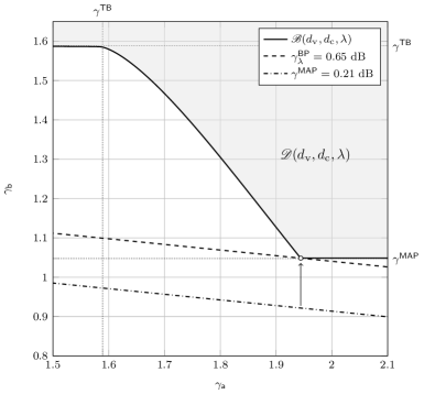
Figure 1: Achievable region for a $(5,10)$ TB SC-LDPC code ensemble with $N=128$ and $\lambda=1/8$.

Figure 2: BP decoding threshold as a function of $\lambda$, compared with the SNR required for rate $R=1/2$, according to (4).

IV Performance Analysis

In the following, results for regular TB SC-LDPC code (ensembles) with energy shaping are presented through EXIT analysis and Monte Carlo simulations. In both cases, windowed decoding [2] has been considered.

We analyze the performance of the proposed scheme by comparing its iterative decoding thresholds with

• the MAP threshold $\gamma^{\mathsf{MAP}}$ of the corresponding $(d_{\mathrm{v}},d_{\mathrm{c}})$ uncoupled ensemble with uniform energy (UE);

• the BP threshold $\gamma^{\mathsf{BL}}$ of the corresponding $(d_{\mathrm{v}},d_{\mathrm{c}})$ uncoupled ensemble with UE;

• the BP threshold $\gamma^{\mathsf{TE}}$ of the corresponding $(d_{\mathrm{v}},d_{\mathrm{c}})$ terminated ensemble with UE.

The analysis is summarized in Table I for the case of $(d_{\mathrm{v}},d_{\mathrm{c}})=(5,10)$. The table provides the thresholds for the different ensembles, for $N=128$, $N=256$, and $N\rightarrow\infty$. For large $N$, the threshold achieved with the proposed approach matches the one of the $(5,10)$ terminated ensemble with UE, saturating to the MAP threshold of the corresponding $(5,10)$ uncoupled ensemble with UE. For moderate-to-small $N$, the proposed approach achieves a larger threshold with respect to the terminated case. However, while for the terminated ensemble the actual coding rate is less than $1/2$ (it reduces to $0.46875$ for $N=128$), the proposed scheme keeps the code rate to the nominal rate. The difference in coding gain between the terminated case and the TB SC-LDPC code ensemble with energy shaping is limited to about $0.16$ dB for $N=128$, and reduces to $0.09$ dB for $N=256$. The gain with respect to the uncoupled ensemble threshold exceeds $1.3$ dB for all cases summarized in Table I. Table II compares the thresholds achieved by various $(d_{\mathrm{v}},d_{\mathrm{c}})$ ensembles for the case of $N=128$. Remarkably, for $N=128$ energy shaping achieves the smallest threshold for the $(4,8)$ ensemble, with a gain of almost $1$ dB over the corresponding block ensemble. This fact has to be attributed to the moderate number of spatial positions $N$, whereas for $N$ growing large the decoding threshold shall improve with increasing VN and CN degrees.

We simulated the performance of the $(5,10)$ TB SC-LDPC code with $N=128$, with and without energy boosting. For the case where energy boosting is employed, the boosting parameters have been set to the values minimizing the BP threshold, i.e., $\lambda=1/8$ (with $\phi=1.85$). The protograph has been expanded with a lifting factor $Q=512$, yielding a block length $n=2^{16}$. For decoding, we employed windowed decoding with $50$ iterations per window position (local iteration), and a window spanning over $16\times Q$ VNs. The window is shifted by $2\times Q$ positions at the end of the local iteration steps, circling twice around the tailbiting Tanner graph. The results, in terms of bit error rate (BER) and codeword error rate (CER), are provided in Fig. 3. A gain close to $1.1$ dB at $\mathrm{CER}=10^{-2}$ over the UE case is achieved.

TABLE I: Comparison of different thresholds for the $(5,10)$ SC-LDPC code ensemble and different $N$.

$N$	$\gamma^{\mathsf{BL}}$ [dB]	$\gamma^{\mathsf{TE}}$ [dB]	$\gamma^{\mathsf{BP}}$ [dB]	$\gamma^{\mathsf{MAP}}$ [dB]
$128$	$2.001\,95$	$0.486$	$0.646\,335\,922\,977$	$0.21$
$256$	$2.001\,95$	$0.343\,704$	$0.431\,596\,511\,332$	$0.21$
$\infty$	$2.001\,95$	$0.21$	$0.21$	$0.21$

TABLE II: Comparison of different SC-LDPC code ensembles and their respective thresholds for $N=128$ and optimal $\lambda$.³

$(d_{\mathrm{v}},d_{\mathrm{c}})$	$\gamma^{\mathsf{BL}}$ [dB]	$\gamma^{\mathsf{TE}}(\Delta)$ [dB]	$\gamma^{\mathsf{BP}}(\Delta)$ [dB]	$\gamma^{\mathsf{MAP}}$ [dB]
$(3,6)$	$1.097\,18$	$$0.592\,85$\,($0.471\,270\,155\,742$)$	$$0.599\,177\,826\,673$\,($0.394\,985\,711\,471$)$	$0.454$
$(4,8)$	$1.538\,24$	$$0.4606$\,($0.372\,784\,750\,540\,4$)$	$$0.539\,419\,360\,066$\,($0.300\,985\,794\,99$)$	$0.25$
$(5,10)$	$2.001\,95$	$$0.486$\,($0.432\,618\,934\,821$)$	$$0.646\,335\,922\,977$\,($0.364\,855\,892\,931$)$	$0.21$
3$\Delta$ is defined as the gap in dB to the corresponding limit according to (4)

V Conclusions

We analyzed the convergence behavior of TB SC-LDPC codes over the bi-AWGN channel with different reliabilities assigned to the codeword bits by shaping the transmission energies. By focusing on the case where only two energy levels are allowed, and a contiguous portion of the codeword is transmitted with the largest energy, we showed that large coding gains (e.g., up to $1.1\text{\ $\mathrm{dB}$}$ for the $(5,10)$ ensemble) can be attained with reference to the case where a uniform energy is employed. The results of the asymptotic analysis are confirmed by finite-length simulations. We conjecture that additional coding gains might be achieved by jointly optimizing the protograph ensemble and the shaping parameters.

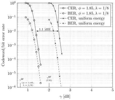
Figure 3: BER and CER vs. average SNR for a $(5,10)$ TB SC-LDPC code with $N=128$ and $n=2^{16}$, with and without energy boosting.

References

- [1] R. Gallager, Low-density parity-check codes. Cambridge, MA, USA: MIT Press, 1963.
- [2] M. Lentmaier, A. Sridharan, D. Costello, Jr., and K. Zigangirov, “Iterative decoding threshold analysis for LDPC convolutional codes,” IEEE Trans. Inf. Theory, vol. 56, no. 10, pp. 5274–5289, Oct. 2010.
- [3] S. Kudekar, T. Richardson, and R. L. Urbanke, “Spatially coupled ensembles universally achieve capacity under belief propagation,” IEEE Trans. Inf. Theory, vol. 59, no. 12, pp. 7761–7813, Dec. 2013.
- [4] D. G. M. Mitchell, M. Lentmaier, and D. J. Costello, “Spatially coupled LDPC codes constructed from protographs,” IEEE Trans. Inf. Theory, vol. 61, no. 9, pp. 4866–4889, Sep. 2015.
- [5] C. Häger, A. Graell i Amat, A. Alvarado, F. Brännström, and E. Agrell, “Optimized bit mappings for spatially coupled LDPC codes over parallel binary erasure channels,” in Proc. IEEE Int. Conf. Commun. (ICC), Sydney, Australia, Jun. 2014, pp. 2064–2069.
- [6] C. Häger, A. Graell i Amat, F. Brännström, A. Alvarado, and E. Agrell, “Terminated and tailbiting spatially coupled codes with optimized bit mappings for spectrally efficient fiber-optical systems,” J. Lightw. Technol., vol. 33, no. 7, pp. 1275–1285, Apr. 2015.
- [7] S. Cammerer, V. Aref, L. Schmalen, and S. ten Brink, “Triggering wave-like convergence of tail-biting spatially coupled LDPC codes,” in 50th Annual Conf. on Information Science and Systems (CISS), Princeton (NJ), USA, March 2016, pp. 93–98.
- [8] M. R. Sanatkar and H. D. Pfister, “Increasing the rate of spatially-coupled codes via optimized irregular termination,” in Proc. 9th Int. Symp. Turbo Codes and Iterative Inf. Processing, Brest, France, Sep. 2016, pp. 121–125.
- [9] G. Forney, R. Gallager, G. Lang, F. Longstaff, and S. Qureshi, “Efficient modulation for band-limited channels,” IEEE J. Sel. Areas Commun., vol. 2, no. 5, pp. 632–647, Sep. 1984.
- [10] G. Liva and M. Chiani, “Protograph LDPC codes design based on EXIT analysis,” in Proc. IEEE Global Telecommun. Conf. (Globecom), Washington (DC), USA, Nov. 2007, pp. 3250–3254.
- [11] P. Pulini, G. Liva, and M. Chiani, “Unequal Diversity LDPC Codes for Relay Channels,” IEEE Trans. Wireless Commun., vol. 12, no. 11, pp. 5646–5655, Nov. 2013.
- [12] J. Thorpe, “Low-density parity-check (LDPC) codes constructed from protographs,” NASA JPL, Pasadena, CA, USA, IPN Progress Report 42-154, Aug. 2003.
- [13] G. Richter and M. Bossert, “Improving the performance of protograph LDPC codes by using different transmission energies,” in Proc. IEEE Int. Symp. Inf. Theory (ISIT), Nice, France, June 2007, pp. 2251–2255.