Blind Source Separation with Optimal Transport Non-negative Matrix Factorization

Abstract

Optimal transport as a loss for machine learning optimization problems has recently gained a lot of attention. Building upon recent advances in computational optimal transport, we develop an optimal transport non-negative matrix factorization (NMF) algorithm for supervised speech blind source separation (BSS). Optimal transport allows us to design and leverage a cost between short-time Fourier transform (STFT) spectrogram frequencies, which takes into account how humans perceive sound. We give empirical evidence that using our proposed optimal transport NMF leads to perceptually better results than Euclidean NMF, for both isolated voice reconstruction and BSS tasks. Finally, we demonstrate how to use optimal transport for cross domain sound processing tasks, where frequencies represented in the input spectrograms may be different from one spectrogram to another.

1 Introduction

Blind source separation (BSS) is the task of separating a mixed signal into different components, usually referred to as sources. In the context of sound processing, it can be used to separate speakers whose voices have been recorded simultaneously. A common way to address this task is to decompose the signal spectrogram by non-negative matrix factorization (NMF, Lee and Seung 2001), as proposed for example by Schmidt and Olsson (2006) as well as Sun and Mysore (2013). Denoting $\tilde{x}_{j,i}$ the (complex) short-time Fourier transform (STFT) coefficient of the input signal at frequency bin $j$ and time frame $i$, and $X$ its magnitude spectrogram defined as $x_{j,i}=|\tilde{x}_{j,i}|$, the BSS problem can be tackled by solving the NMF problem

$$\min_{D^{(1)}\dots D^{(N)},\,W^{(1)}\dots W^{(N)}}\sum_{i=1}^{t}\ell\left(\boldsymbol{x}_{i},\sum_{k=1}^{N}D^{(k)}\boldsymbol{w}_{i}^{(k)}\right)$$ (1)

where $N$ is the number of sources, $t$ is the number of time windows, $\boldsymbol{x}_{i}$ is the $i$^th column of $X$ and $\ell$ is a loss function. Each dictionary matrix $D^{(k)}$ and weight matrix $W^{(k)}$ are related to a single source. In a supervised setting, each source has training data and all the $D^{(k)}$s are learned in advance during a training phase. At test time, given a new signal, separated spectrograms are recovered from the $D^{(k)}$s and $W^{(k)}$s and corresponding signals can be reconstructed with suitable post-processing. Several loss functions $\ell$ have been considered in the literature, such as the squared Euclidean distance (Lee and Seung 2001; Schmidt and Olsson 2006), the Kullback-Leibler divergence (Lee and Seung 2001; Sun and Mysore 2013) or the Itakura-Saito divergence (Févotte et al. 2009; Sawada et al. 2013).

In the present article, we propose to use optimal transport as a loss between spectrograms to perform supervised speech BSS with NMF. Optimal transport is defined as the minimum cost of moving the mass from one histogram to another. By taking into account a transportation cost between frequencies, this provides a powerful metric to compare STFT spectrograms. One of the main advantage of using optimal transport as a loss is that it can quantify the amplitude of a frequency shift noise, coming for example from quantization or the tuning of a musical instrument. Other metrics such as the Euclidean distance or Kullback-Leibler divergence, which compare spectrograms element-wise, are almost blind to this type of noise (see Figure 1). Another advantage over element-wise metrics is that optimal transport enables the use of different quantizations, i.e. frequency supports, at training and test times. Indeed, the frequencies represented on a spectrogram depend on the sampling rate of the signal and the time-windows used for its computation, both of which can change between training and test times. With optimal transport, we do not need to re-quantize the training and testing data so as they share the same frequency support: optimal transport is well-defined between spectrograms with distinct supports as long as we can define a transportation cost between frequencies. Finally, the optimal transport framework enables us to generalize the Wiener filter, a common post-processing for source separation, by using optimal transport plans, so that it can be applied to data quantized on different frequencies.

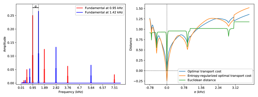
Figure 1: Comparison of Euclidean distance and (regularized) optimal transport losses. Synthetic musical notes are generated by putting weight on a fundamental, and exponentially decreasing weights on its harmonics and sub-harmonics, and finally convoluting with a Gaussian. Left: examples of the spectrograms of two such notes. Right: (regularized) optimal transport loss and Euclidean distance from the note of fundamental $0.95$kHz (red line on the left plot) to the note of fundamental $0.95$kHz$+\sigma$, as functions of $\sigma$. The Euclidean distance varies sharply whereas the optimal transport loss captures more smoothly the change in the fundamental. The variations of the optimal transport loss and its regularized version are similar, although the regularized one can become negative.

NMF with an optimal transport loss was first proposed by Sandler and Lindenbaum (2009). They solved this problem by using a bi-convex formulation and relied on an approximation of optimal transport based on wavelets (Shirdhonkar and Jacobs 2008). Recently, Rolet et al. (2016) proposed fast algorithms to compute NMF with an entropy-regularized optimal transport loss, which are more flexible in the sense that they do not require any assumption on the frequency quantization or on the cost function used.

Using optimal transport as a loss between spectrograms was also proposed by Flamary et al. (2016) under the name “optimal spectral transportation”. They developed a novel method for unsupervised music transcription which achieves state-of-the-art performance. Their method relies on a cost matrix designed specifically for musical instruments, allowing them to use Diracs as dictionary columns. That is, they fix each dictionary column to a vector with a single non-zero entry and learn only the corresponding coefficients. This trivial structure of the dictionary results in efficient coefficient computation. However, this approach cannot be applied as is to speech separation since it relies on the assumption that a musical note can be represented as its fundamental. It also requires designing the cost of moving the fundamental to its harmonics and neighboring frequencies. Because human voices are intrinsically more complex, it is therefore necessary to learn both the dictionary and the coefficients, i.e., solve full NMF problems.

Our contributions

In this paper, we extend the optimal transport NMF of Rolet et al. (2016) to the case where the columns of the input matrix $X$ are not normalized in order to propose an algorithm which is suitable for spectrogram data. Normalizing all time frames so that they have the same total weight is not desirable in sound processing tasks because it would amplify noise. We define a cost between frequencies so that the optimal transport objective between spectrograms provides a relevant metric between them. We apply our NMF framework to single voice reconstruction and blind source separation and show that an optimal transport loss provides better results over the usual squared Euclidean loss. Finally, we show how to use our framework for cross domain BSS, where frequencies represented in the test spectrograms may be different from the ones in the dictionary. This may happen for example when train and test data are recorded with different equipment, or when the STFT is computed with different parameters.

Notations

We denote matrices in upper-case, vectors in bold lower-case and scalars in lower-case. If $M$ is a matrix, $M^{\top}$ is its transpose, $\boldsymbol{m}_{i}$ is its $i$^th column and $\boldsymbol{m}_{j:}$ its $j$^th row. $\boldsymbol{1}_{n}$ denotes the all-ones vector in $\mathbb{R}^{n}$; when the dimension can be deduced from context we simply write $\boldsymbol{1}$. For two matrices $A$ and $B$ of the same size, we denote their inner product $\left<A,B\right>\coloneqq\operatorname{tr}\left(A^{\top}B\right)$. We denote $\Sigma_{n}$ the $(n-1)$-dimensional simplex: $\Sigma_{n}\coloneqq\left\{\boldsymbol{x}\in\mathbb{R}_{+}^{n}\colon\|\boldsymbol{x}\|_{1}=1\right\}$.

2 Background

We start by introducing optimal transport, its entropy regularization, which we will use as the loss $\ell$, and previous works on optimal transport NMF. For a more comprehensive overview of optimal transport from a computational perspective, see Peyré and Cuturi (2017).

2.1 Optimal Transport

Exact Optimal Transport.  Let $\boldsymbol{a}\in\Sigma_{m},\,\boldsymbol{b}\in\Sigma_{n}$. The polytope of transportation matrices between $\boldsymbol{a}$ and $\boldsymbol{b}$ is defined as

$$U(\boldsymbol{a},\boldsymbol{b})\coloneqq\left\{T\in\mathbb{R}_{+}^{m\times n}\left|\begin{aligned} T\boldsymbol{1}=\boldsymbol{a}\\ T^{\top}\boldsymbol{1}=\boldsymbol{b}\end{aligned}\right.\right\}.$$

Given a cost matrix $C\in\mathbb{R}^{m\times n}$, the minimum transportation cost between $\boldsymbol{a}$ and $\boldsymbol{b}$ is defined as

$$\operatorname{OT}(\boldsymbol{a},\boldsymbol{b})=\min_{T\in U(\boldsymbol{a},\boldsymbol{b})}\left<T,C\right>.$$ (2)

When $n=m$ and the cost matrix is the $p$-th power ($p\geqslant 1$) of a distance matrix, i.e. $c_{i,j}=d(\boldsymbol{y}_{i},\boldsymbol{y}_{j})^{p}$ for some $(\boldsymbol{y}_{i})$ in a metric space $(\Omega,\,d)$, then $\operatorname{OT}(\cdot,\cdot)^{1/p}$ is a distance on the set of vectors in $\mathbb{R}_{+}^{n}$ with the same $\ell$-$1$ norm (Villani 2003 Theorem 7.3). We can see the vectors $\boldsymbol{y}_{i}$ as features, and $\boldsymbol{a}$ and $\boldsymbol{b}$ as the quantization weights of the data onto these features. In sound processing applications, the vectors $\boldsymbol{y}_{i}$ are real numbers corresponding to the frequencies of the spectrogram and $\boldsymbol{a}$ and $\boldsymbol{b}$ are their corresponding magnitude. By computing the minimal transportation cost between frequencies of two spectrograms, optimal transport exhibits variations in accordance with the frequency noise involved in the signal generative process, which results for instance from the tuning of musical instruments or the subject’s condition in speech processing.

Unnormalized Optimal Transport.  In this work, we wish to define optimal transport when $\boldsymbol{a}$ and $\boldsymbol{b}$ are non-negative but not necessarily normalized. Note that the transportation polytope is not empty as long as $\boldsymbol{a}$ and $\boldsymbol{b}$ sum to the same value: $U(\boldsymbol{a},\boldsymbol{b})=\emptyset$ iif $\|\boldsymbol{a}\|_{1}\neq\|\boldsymbol{b}\|_{1}$. Hence, we define optimal transport between possibly unnormalized vectors $\boldsymbol{a}$ and $\boldsymbol{b}$ as,

$$\operatorname{OT}(\boldsymbol{a},\boldsymbol{b})\coloneqq\left\{\begin{aligned} &\min_{T\in U(\boldsymbol{a},\boldsymbol{b})}\left<T,C\right>&&\mbox{if }\|\boldsymbol{a}\|_{1}=\|\boldsymbol{b}\|_{1}\mbox{ and }\boldsymbol{a},\boldsymbol{b}\geq 0;\\ &\infty&&\mbox{otherwise}.\end{aligned}\right.$$ (3)

Computing the optimal transport cost (3) amounts to solve a linear program (LP) which can be done with specialized versions of the simplex algorithm with worst-case complexity in $\mathcal{O}(n^{3}\log n)$ when $n=m$ (Orlin 1997). When considering $\operatorname{OT}$ as a loss between histograms supported on more than a few hundred bins, such computation becomes quickly intractable. Moreover, using $\operatorname{OT}$ as a loss involves differentiating $\operatorname{OT}$, which is not differentiable everywhere. Hence, one would have to resort to subgradient methods. This would be prohibitively slow since each iteration would require to obtain a subgradient at the current iterate, which requires to solve the LP (3).

Entropy Regularized Optimal Transport.  To remedy these limitations, Cuturi (2013) proposed to add an entropy-regularization term to the optimal transport objective, thus making the $\operatorname{OT}$ loss differentiable everywhere and strictly convex. This entropy-regularized optimal transport has since been used in numerous works as a loss for diverse tasks (see for example Gramfort et al. 2015; Frogner et al. 2015; Rolet et al. 2016).

Let $\gamma>0$, we define the (unnormalized) entropy-regularized OT between $\boldsymbol{a}\in\mathbb{R}_{+}^{m},\,\boldsymbol{b}\in\mathbb{R}_{+}^{n}$ as

$$\operatorname{OT}_{\gamma}(\boldsymbol{a},\boldsymbol{b})\coloneqq\left\{\begin{aligned} &\min_{T\in U(\boldsymbol{a},\boldsymbol{b})}&&\left<T,C\right>-\gamma E(T)&&\mbox{ if}\quad\|\boldsymbol{a}\|_{1}=\|\boldsymbol{b}\|_{1}\mbox{ and }\boldsymbol{a},\boldsymbol{b}\geq 0;\\ &&&\infty&&\mbox{otherwise.}\end{aligned}\right.$$ (4)

where $E(T)\coloneqq\sum_{ij}T_{ij}\log{T_{ij}}$ is the entropy of the transport plan $T$. Let us denote $\operatorname{OT}_{\gamma}^{\star}$ the convex conjugate of $\operatorname{OT}_{\gamma}$ with respect to its second variable

$$\operatorname{OT}_{\gamma}^{\star}(\boldsymbol{x},\boldsymbol{y})=\max_{\begin{subarray}{c}\boldsymbol{z}\geq 0\\ \|\boldsymbol{z}\|_{1}=\|\boldsymbol{x}\|_{1}\end{subarray}}\left<\boldsymbol{y},\boldsymbol{z}\right>-\operatorname{OT}_{\gamma}(\boldsymbol{x},\boldsymbol{z}).$$

Cuturi and Peyré (2016) showed that its value and gradient can be computed in closed-form:

$$\operatorname{OT}_{\gamma}^{\star}(\boldsymbol{x},\boldsymbol{y})=\gamma\left(E(\boldsymbol{x})+\left<\boldsymbol{x},\log K\boldsymbol{\alpha}\right>\right),$$

$$\nabla_{\boldsymbol{y}}\operatorname{OT}_{\gamma}^{\star}(\boldsymbol{x},\boldsymbol{y})=\boldsymbol{\alpha}\odot\left(K^{\top}\frac{\boldsymbol{x}}{K\boldsymbol{\alpha}}\right),$$

where $K\coloneqq e^{-C/\gamma}$ and $\boldsymbol{\alpha}\coloneqq e^{\boldsymbol{y}/\gamma}$.

2.2 Optimal Transport NMF

NMF can be cast as an optimization problem of the form

$$\min_{D\in\mathbb{R}_{+}^{n\times k},\,W\in\mathbb{R}_{+}^{k\times t}}\sum_{i=1}^{t}\ell(\boldsymbol{x}_{i},D\boldsymbol{w}_{i})+R(W,D),$$ (5)

where both $D$ and $W$ are optimized at train time, and $D$ is fixed at test time. When $\ell$ is $\operatorname{OT}$, problem (5) is convex in $W$ and $D$ separately, but not jointly. It can be solved by alternating full optimization with respect to $W$ and $D$. Each resulting sub-problem is a very high dimensional linear program with many constraints (Sandler and Lindenbaum 2009), which is intractable with standard LP solvers even for short sound signals. In addition, convergence proofs of alternate minimization methods for NMF typically assume strictly convex sub-problems (see e.g.  Tropp 2003; Bertsekas 1999 Prop. 2.7.1), which is not the case when using non-regularized $\operatorname{OT}$ as a loss.

To address this issue, Rolet et al. (2016) proposed to use $\operatorname{OT}_{\gamma}$ instead, and showed how to solve each sub-problem in the dual using fast gradient computations. Formally, they tackle problems of the form:

$$\min_{\begin{subarray}{c}D\in\Sigma_{n}^{k}\\ W\in\Sigma_{k}^{t}\end{subarray}}\sum_{i=1}^{t}\operatorname{OT}_{\gamma}(\boldsymbol{x}_{i},D\boldsymbol{w}_{i})+R_{1}(\boldsymbol{w}_{i})+\sum_{i=1}^{k}R_{2}(\boldsymbol{d}_{i})$$ (6)

where $R_{1}$ and $R_{2}$ are convex regularizers that enforce non-negativity constraints, and $\Sigma_{n}$ is the $(n-1)$-dimensional simplex.

It was shown that each sub-problem of (6) with either $D$ or $W$ fixed has a smooth Fenchel-Rockafellar dual, which can be solved efficiently, leading to a fast overall algorithm. However, their definition of optimal transport requires inputs and reconstructions to have a $\ell$-$1$ norm equal to $1$. This is achieved by normalizing the input beforehand, restricting the columns of $D$ and $W$ to the simplex, and using as regularizers negative entropies defined on the simplex:

$$R_{1}(W)\coloneqq R(\rho_{1},W)\quad\text{and}\quad R_{2}(W)\coloneqq R(\rho_{2},W)$$ (7)

where

$$R(\rho,W)\coloneqq\begin{cases}-\rho E(W)&\mbox{ if }\|\boldsymbol{w}_{i}\|_{1}=1,\,\forall i\\ \infty&\mbox{ otherwise.}\end{cases}.$$ (8)

They showed that the coefficients and dictionary can be updated according to the following duality results.

Coefficients Update.  For $D$ fixed, the optimizer of

$$\min_{\begin{subarray}{c}W\in\Sigma_{k}^{t}\\ \forall i,\,D\boldsymbol{w}_{i}=\boldsymbol{x}_{i}\end{subarray}}\displaystyle\sum_{i=1}^{t}\operatorname{OT}_{\gamma}(\boldsymbol{x}_{i},D\boldsymbol{w}_{i})+R_{1}(\boldsymbol{w}_{i})$$

is

$$W^{*}=\left(\frac{e^{-D^{\top}\boldsymbol{g}_{i}^{*}/\rho_{1}}}{\left<e^{-D^{\top}\boldsymbol{g}_{i}^{*}/\rho_{1}},\boldsymbol{1}\right>}\right)_{i=1}^{m}$$ (9)

with

$$\boldsymbol{g}_{i}^{*}\in\operatorname*{argmin}_{\boldsymbol{g}\in\mathbb{R}^{s}}\,\operatorname{OT}_{\gamma}^{\star}(\boldsymbol{x}_{i},\boldsymbol{g})+R_{1}^{\star}(-D^{\top}\boldsymbol{g}).$$ (10)

We can solve Problem (10) with accelerated gradient descent (Nesterov 1983), and recover the optimal weight matrix with the primal-dual relationship (9). The value and gradient of the convex conjugate of $R$ with respect to its second variable are:

$$R^{\star}(\rho,\boldsymbol{x})=\rho\log\left<e^{\boldsymbol{x}/\rho},\mathbf{1}\right>$$

$$\nabla_{x}R^{\star}(\rho,\boldsymbol{x})=\frac{e^{\boldsymbol{x}/\rho}}{\left<e^{\boldsymbol{x}/\rho},\mathbf{1}\right>}.$$

Dictionary Update.  For $W$ fixed, the optimizer of

$$\min_{\begin{subarray}{c}D\in\Sigma_{m}^{k}\\ \forall i,\,D\boldsymbol{w}_{i}=\boldsymbol{x}_{i}\end{subarray}}\displaystyle\sum_{i=1}^{t}\operatorname{OT}_{\gamma}(\boldsymbol{x}_{i},D\boldsymbol{w}_{i})+\sum_{i=1}^{k}R_{2}(\boldsymbol{d}_{i})$$

is

$$D^{*}=\left(\frac{e^{-G^{*}\boldsymbol{w}_{i:}^{\top}/\rho_{2}}}{\left<e^{-G^{*}\boldsymbol{w}_{i:}^{\top}/\rho_{2}},\mathbf{1}\right>}\right)_{i=1}^{k}$$ (11)

with

$$G^{*}\in\operatorname*{argmin}_{G\in\mathbb{R}^{n\times t}}\displaystyle\sum_{i=1}^{t}\operatorname{OT}_{\gamma}^{\star}(\boldsymbol{x}_{i},\boldsymbol{g}_{i})+\displaystyle\sum_{i=1}^{k}R_{2}^{\star}(-G\boldsymbol{w}_{i:}^{\top}).$$ (12)

Likewise, we can solve Problem (12) with accelerated gradient descent, and recover the optimal dictionary matrix with the primal-dual relationship (11).

These duality results allow us to go from a constrained primal problem for which each evaluation of the objective and its gradient requires solving an optimal transport problem, to a non-constrained dual problem whose objective and gradient can be evaluated in closed form. The primal constraints $\|\boldsymbol{x}_{i}\|_{1}=\|D\boldsymbol{w}_{i}\|_{1}$ and $D\boldsymbol{w}_{i}\geq 0$ $\forall i$ are enforced by the primal-dual relationship. Moreover, the use of an entropy regularization, with $\gamma>0$, makes $\operatorname{OT}_{\gamma}$ smooth with respect to its second variable.

3 Method

We now present our approach for optimal transport BSS. First we introduce the changes to Rolet et al. (2016) that are necessary for computing optimal transport NMF on STFT spectrograms of sound data. We then define a transportation cost between frequencies. Finally we show how to reconstruct sound signals from the separated spectrograms.

3.1 Signal Separation With NMF

We use a supervised BSS setting similar to the one described in Schmidt and Olsson (2006). For each source $k$ we have access to training data $X^{(k)}$, on which we learn a dictionary $D^{(k)}$ with NMF

$$\min_{W,D^{(k)}}\sum_{i=1}^{t}\ell(\boldsymbol{x}_{i},D^{(k)}\boldsymbol{w}_{i})+R_{1}(W)+R_{2}(D^{(k)}).$$

Then, given the STFT spectrum of a mixture of voices $X$, we reconstruct separated spectrograms $X^{(k)}=D^{(k)}W^{(k)}$ for $k=1,\dots N$ where $W^{(k)}$sare the solutions of

$$\min_{W^{(1)},\dots,W^{(N)}}\sum_{i=1}^{t}\ell(\boldsymbol{x}_{i},\sum_{k=1}^{N}D^{(k)}\boldsymbol{w}_{i}^{(k)})+\sum_{k=1}^{N}R_{1}(W^{(k)}).$$

The separated signals are then reconstructed from each $X^{(k)}$ with the process described in Section 3.4.

In practice at test time, the dictionaries are concatenated in a single matrix $D=(D^{(k)})_{k=1}^{N}$, and a single matrix of coefficients $W$ is learned, which we decompose as $W=(W^{(k)})_{k=1}^{N}$. This allows us to focus on problems of the form

$$\min_{W,D}\sum_{i=1}^{t}\ell(\boldsymbol{x}_{i},D\boldsymbol{w}_{i})+R_{1}(W)+R_{2}(D).$$

3.2 Non-normalized Optimal Transport NMF

Normalizing the columns of the input $X$, as in Rolet et al. (2016), is not a good option in the context of signal processing, since frames with low amplitudes are typically noise and it would amplify them.

However, our definition of optimal transport does not require inputs to be in the simplex, only to have the same $\ell$-$1$ norm. With this definition, the convex conjugate $\operatorname{OT}^{\star}$ of $\operatorname{OT}$ and its gradient still have the same value as in Cuturi and Peyré (2016), and we can simply relax the condition on $W$ to be $W\geq 0$ in Problem (6). We keep a simplex constraint on the columns of the dictionary $D$ so that each update is guaranteed to stay in a compact set. We use $R_{1}=-\rho_{1}E$, a negative entropy defined on the non-negative orthant as the coefficient matrix regularizer and for $R_{2}$ we keep the non-negative entropy defined on the simplex. The problem then becomes

$$\min_{\begin{subarray}{c}D\in\Sigma_{n}^{k}\\ W\in\mathbb{R}_{+}^{k\times t}\end{subarray}}\sum_{i=1}^{t}\operatorname{OT}_{\gamma}(\boldsymbol{x}_{i},D\boldsymbol{w}_{i})+R_{1}(\boldsymbol{w}_{i})+\sum_{i=1}^{k}R_{2}(\boldsymbol{d}_{i})$$ (13)

The dictionary update is the same as in Rolet et al. (2016). However, the coefficient updates need to be modified as follows.

Coefficients Update.  For $D$ fixed, the optimizer of

$$\min_{\begin{subarray}{c}W\in\mathbb{R}_{+}^{k\times t}\\ \forall i,\,D\boldsymbol{w}_{i}=\boldsymbol{x}_{i}\end{subarray}}\displaystyle\sum_{i=1}^{t}\operatorname{OT}_{\gamma}(\boldsymbol{x}_{i},D\boldsymbol{w}_{i})+R_{1}(\boldsymbol{w}_{i})$$

is $W^{*}=\left(e^{-D^{\top}\boldsymbol{g}_{i}^{*}/\rho_{1}-1}\right)_{i=1}^{m}$, with

$$\boldsymbol{g}_{i}^{*}\in\operatorname*{argmin}_{\boldsymbol{g}\in\mathbb{R}^{s}}\,\operatorname{OT}_{\gamma}^{\star}(\boldsymbol{x}_{i},\boldsymbol{g})+R_{1}^{\star}(-D^{\top}\boldsymbol{g}).$$ (14)

The concave conjugate of $E$ and its gradient can be evaluated with:

$$R_{1}^{\star}(\boldsymbol{x})=\rho_{1}\left<e^{\boldsymbol{x}/\rho_{1}-1},\mathbf{1}\right>$$

$$\nabla R_{1}^{\star}(\boldsymbol{x})=e^{\boldsymbol{x}/\rho_{1}-1}.$$

3.3 Cost Matrix Design

In order to compute optimal transport on spectrogams and perform NMF, we need a cost matrix $C$, which represents the cost of moving weight from frequencies in the original spectrogram to frequencies in the reconstructed spectrogram. Schmidt and Olsson (2006) use the mel scale to quantize spectrograms, relying on the fact that the perceptual difference between frequencies is smaller for the high frequency than for the low frequency domain. Following the same intuition, we propose to map frequencies to a log-domain and apply a cost function in that domain. Let $f_{j}$ be the frequency of the $j$-th bin in an input data spectrogram, where $1\leq j\leq m$. Let $\hat{f}_{\hat{j}}$ be the frequency of the $\hat{j}$-th bin in a reconstruction spectrogram, where $1\leq\hat{j}\leq n$. We define the cost matrix $C\in\mathbb{R}^{m\times n}$ as

$$c_{j\hat{j}}=\left|\log(\lambda+f_{j})-\log(\lambda+\hat{f}_{\hat{j}})\right|^{p}$$ (15)

with parameters $\lambda\geq 0$ and $p>0$. Since the mel scale is a log scale, it is included in this definition for some parameter $\lambda$. Some illustrations of our cost matrix for different values of $\lambda$ are shown in Figure 2, with $p=0.5$. It shows that with our definition, moving weights locally is less costly for high frequencies than low ones, and that this effect can be tuned by selecting $\lambda$.

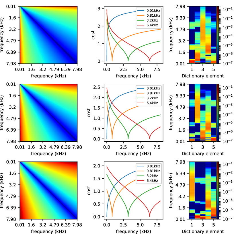
Figure 2: $\lambda$ parameter of the Cost Matrix. Influence of parameter $\lambda$ of the cost matrix. Left: cost matrix; center: sample lines of the cost matrix; right: dictionary learned on the validation data. Top: $\lambda=1$; center: $\lambda=100$; bottom: $\lambda=1000$.

Figure 3 shows the effect of $p$ on the learned dictionaries. Using $p=0.5$ yields a cost that is more spiked, leading to dictionary elements that can have several spikes in the same frequency bands, whereas $p\geq 1$ tends to produce smoother dictionary elements.

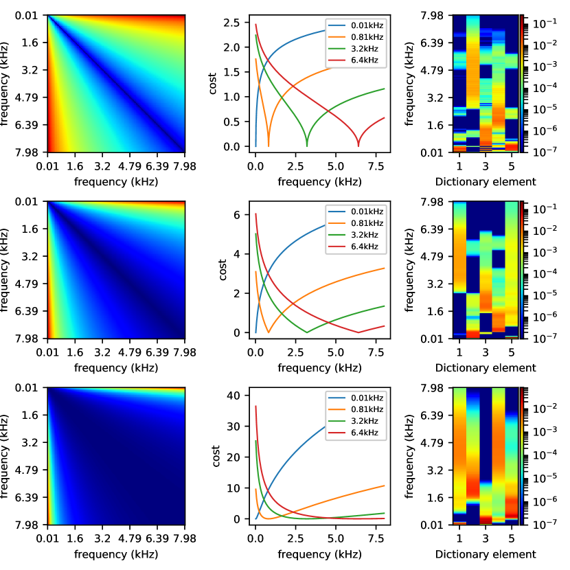
Figure 3: Power of the Cost Matrix. Influence of the power $p$ of the cost matrix. Left: cost matrix; center: sample lines of the cost matrix; right: dictionary learned on the validation data. Top: $p=0.5$; center: $p=1$; bottom: $p=2$.

Note that with this definition and $p\geq 1$ , $C$ is a distance matrix to the power $p$ when the source and target frequencies are the same. If $p=0.5$, $C$ is the point-wise square-root of a distance matrix and as such is a distance matrix itself. $\operatorname{OT}(.,.)^{1/p}$.

Parameters $p=0.5$ and $\lambda=100$ yielded better results for Blind Source Separation on the validation set and were accordingly used in all our experiments.

3.4 Post-processing

Wiener Filter.  In the case where the reconstruction is in the same frequency domain as the original signal, the classical way to recover each voice in the time domain is to apply a Wiener filter. Let $X$ be the original Fourier spectrum, $X^{(1)}$ and $X^{(2)}$ the separated spectra such that $X\approx X^{(1)}+X^{(2)}$. The Wiener filter builds $\hat{X^{(1)}}=X\odot\frac{X^{(1)}}{X^{(1)}+X^{(2)}}$ and $\hat{X^{(2)}}=X\odot\frac{X^{(2)}}{X^{(1)}+X^{(2)}}$, before applying the original spectra’s phase and performing the inverse STFT.

Generalized Filter.  We propose to extend this filtering to the case where $X^{(1)}$ and $X^{(2)}$ are not in the same domain as $X$. This may happen for example if the test data is recorded using a different sample frequency, or if the STFT is performed with a different time-window than the train data. In such a case, $D^{(1)}$ and $D^{(2)}$ are in the domain of the train data, and to are $X^{(1)}$ and $X^{(2)}$, but $X$ is in a different domain, and its coefficients correspond to different sound frequencies. As such, we cannot use Wiener filtering.

Instead we propose to use the optimal transportation matrices to produce separated signals $\hat{X^{(1)}}$ and $\hat{X^{(2)}}$ in the same domain as $X$. Let $T_{(i)}\in\displaystyle\operatorname*{argmin}_{\Pi\in U(\boldsymbol{x}_{i},\boldsymbol{x}_{i}^{(1)}+\boldsymbol{x}_{i}^{(2)})}\left<C,\Pi\right>$. With Weiner filtering, $x_{i}$ is decomposed into its components generated by $x_{1}^{(1)}$ and $x_{2}^{(2)}$. We use the same idea and separate the transport matrix $T_{(i)}$ into:

$$T^{(1)}_{(i)} =T_{(i)}\operatorname{diag}\left(\frac{\boldsymbol{x}_{i}^{(1)}}{\boldsymbol{x}_{i}^{(1)}+\boldsymbol{x}_{i}^{(2)}}\right)$$

$$T^{(2)}_{(i)} =T_{(i)}\operatorname{diag}\left(\frac{\boldsymbol{x}_{i}^{(2)}}{\boldsymbol{x}_{i}^{(1)}+\boldsymbol{x}_{i}^{(2)}}\right)$$

$T^{(1)}_{(i)}$ (resp. $T^{(1)}_{(i)}$) is a transport matrix between $\frac{\boldsymbol{x}_{i}^{(1)}}{\boldsymbol{x}_{i}^{(1)}+\boldsymbol{x}_{i}^{(2)}}$ (resp. $\frac{\boldsymbol{x}_{i}^{(2)}}{\boldsymbol{x}_{i}^{(1)}+\boldsymbol{x}_{i}^{(2)}}$) and $\hat{\boldsymbol{x}_{i}}^{(1)}$ (resp. $\hat{\boldsymbol{x}_{i}}^{(2)}$), where

$$\hat{\boldsymbol{x}_{i}}^{(1)} =T^{(i)}\frac{\boldsymbol{x}_{i}^{(1)}}{\boldsymbol{x}_{i}^{(1)}+\boldsymbol{x}_{i}^{(2)}}$$

$$\hat{\boldsymbol{x}_{i}}^{(2)} =T^{(i)}\frac{\boldsymbol{x}_{i}^{(2)}}{\boldsymbol{x}_{i}^{(1)}+\boldsymbol{x}_{i}^{(2)}}$$

Similarly to the classical Wiener filter, we have

$$\hat{\boldsymbol{x}_{i}}^{(1)}+\hat{\boldsymbol{x}_{i}}^{(2)} =T^{(i)}\frac{\boldsymbol{x}_{i}^{(1)}}{\boldsymbol{x}_{i}^{(1)}+\boldsymbol{x}_{i}^{(2)}}+T^{(i)}\frac{\boldsymbol{x}_{i}^{(2)}}{\boldsymbol{x}_{i}^{(1)}+\boldsymbol{x}_{i}^{(2)}}$$

$$=T^{(i)}\boldsymbol{1}$$

$$=\boldsymbol{x}_{i}$$

Heuristic Mapping.  As an alternative to this generalized filter, we propose to simply map the reconstructed signal to the same domain as $X$ by assigning the weight of a $\hat{f}_{j}$ in a spectrogram to its closest neighbor in $(f_{i})_{i=1}^{n}$, according to the distance we defined for the cost matrix (see Section 3.3).

Separated Signal Reconstruction.  Separated sounds are reconstructed by inverse STFT after applying a Wiener filter or generalized filter to $X^{(1)}$ and $X^{(2)}$.

4 Results

In this section we present the main empirical findings of this paper. We start by describing the dataset that we used and the pre-processing we applied to it. We then show that the optimal transport loss allows us to have perceptually good reconstructions of single voices, even with few dictionary elements. Finally we show that the optimal transport loss improves upon a Euclidean loss for BSS with an NMF model, both in single-domain and cross-domain settings.

4.1 Dataset and Pre-processing

We evaluate our method on the English part of the Multi-Lingual Speech Database for Telephonometry 1994 dataset. The data consists of recordings of the voice of four males and four females pronouncing each 24 different English sentences. We split each person’s audio file time-wise into $25\%$-$75\%$ train-test data. The files are re-sampled to $16kHz$ and treated as mono signal.

One of the male voices and one of the female voices are only used for hyper-parameter selection, and are not included in the results.

The signals are analysed by STFT with a Hann window, and a window-size of $1024$, leading to $513$ frequency bins ranging from $0$ to $8$kHz. The constant coefficient is removed from the NMF analysis and added for reconstruction in post-processing.

Hyper-parameters are selected on validation data consisting if the first male and female voice, which are excluded from the evaluation set.

Initialization is performed by setting each dictionary column to the optimal transport barycenter of all the time frames of the training data, to which we added Gaussian noise (separately for each column). The barycenters are computed using the algorithm of Benamou et al. (2015).

4.2 NMF Audio Quality

We first show that using an optimal transport loss for NMF leads to better perceptual reconstruction of voice data. To that end, we evaluated the PEMO-Q score (Huber and Kollmeier 2006) of isolated test voices. The dictionaries are learned on the isolated voices in the train dataset, and are the same as in the following separation experiment.

Figure 4 shows the mean and standard deviation of the scores for $k\in\{5,\,10,\,15,\,20\}$ with optimal transport and Euclidean NMF. The PEMO-Q score of optimal transport NMF is significantly higher for any value of $k$. We found empirically that other scores such as SDR or SNR tend to be better for the Euclidean NMF, even though the reconstructed voices are clearly worse when listening to them (see additional files 1 and 2). Optimal transport can reconstruct clear and intelligible voices with as few as $5$ dictionary elements.

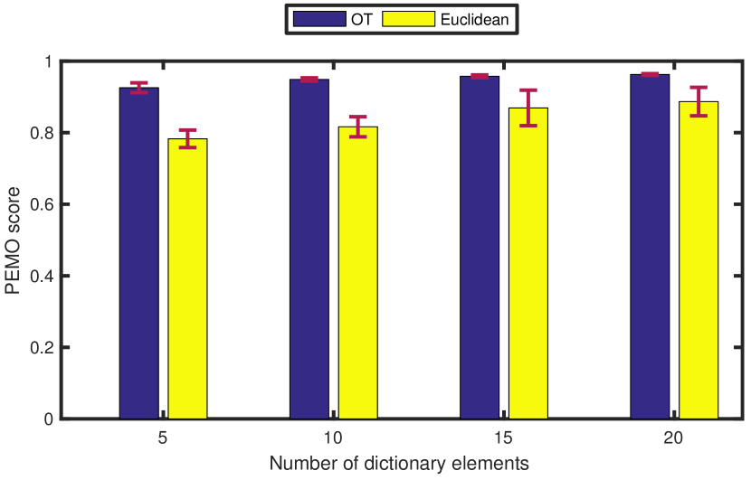
Figure 4: Perceptive Quality Score. Average and standard deviation of PEMO scores of non-mixed voices with optimal transport (blue) or Euclidean (yellow) NMF.

4.3 Blind Source Separation

We evaluate our Blind Source Separation using the PEASS score proposed in Emiya et al. (2011), which they claim is closer to how humans would score BSS than SDR. We only consider mixtures of two voices, where the mixture is simply an addition of the sound signals.

Single-Domain Blind Source Separation. We first show that using an optimal transport NMF improves on Euclidean NMF for BSS using the same frequencies in the spectrogram of the train and test data. In this experiment, both the training and test data are processed in exactly the same way, so that at train and test time $(f_{i})_{i}=(\hat{f}_{i})_{i}$. For Euclidean-based BSS, we reconstruct the signal using a Wiener filter before applying inverse STFT. For optimal transport-based source separation, we evaluate separation using either the Wiener filter or our generalized filter.

Figure 5 shows mean and standard deviation of the PEASS scores for $k\in\{5,\,10,\,15,\,20\}$. The scores are higher with $k=5$ or $k=10$ and in both cases optimal transport yields better results.

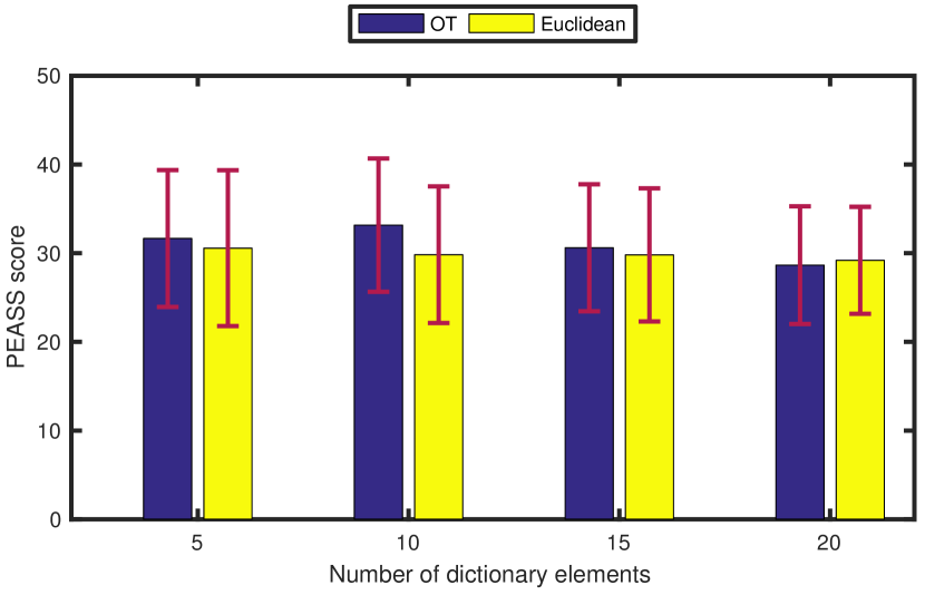
Figure 5: Average Separation Score. Average and standard deviation of PEASS scores with optimal transport (blue) or Euclidean (yellow) NMF, both reconstructed with the Wiener filter.

Figure 6 shows a comparison for each pair of mixed voices, with $k$ selected on the validation set ($k=5$ for Euclidean and $k=10$ for optimal transport NMF). It shows that the PEASS score is better with an optimal transport loss for almost all files. We can further see that in the case of single domain BSS, the Wiener filter and our generalized Wiener filter yields very similar results.

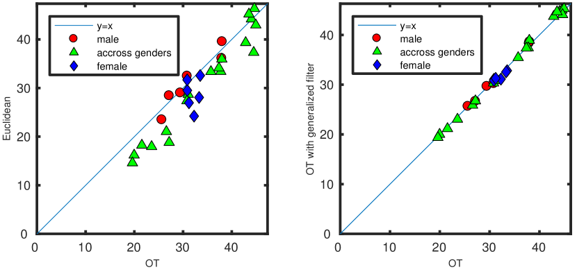
Figure 6: Single Domain Separation Score. Comparison between optimal transport NMF and Euclidean NMF(left) or optimal transport NMF with generalized Wiener filter (right). Each data-point represents the PEASS scores of one file when mixed with another, where the x coordinate is the optimal transport with Wiener filter’s score and the y coordinate is the score of the compared method.

Cross-Domain Blind Source Separation.  In this experiment, we keep the dictionaries trained for the single domain experiment, but we re-process the test data with a different time-window of $600$ for the STFT. Although $(f_{i})_{i}\neq(\hat{f}_{i})_{i}$, we can still compute optimal transport between the spectrograms thanks to our cost matrix.

Figure 7 shows the resuts on the train set. The score for Euclidean NMF is computed by first mapping the test data to the same domain as the train data, using heuristic mapping, and then performing same-domain separation. Both the heuristice mapping and generalized filter improve upon using Euclidean NMF, and they both achieve similar results. Still, the use of our generalized filter allows to have the exact same processing whether performing single domain or cross domain separation, the only difference being the cost matrix $C$, while the heuristic mapping requires additional post-processing and also requires to choose rules for the mapping.

Figure 7: Cross Domain Separation Score. Comparison between optimal transport NMF with generalized Wiener filter and Euclidean NMF (left) or optimal transport NMF with heuristic mapping (right) on the cross domain speech separation task. Each data-point represents the PEASS scores of one file when mixed with another, where the x coordinate is the optimal transport with generalized Wiener filter’s score and the y coordinate is the score of the compared method.

5 Discussion

Regularization of the Transport Plan.  In this work we considered entropy-regularized optimal transport as introduced by Cuturi (2013). This allows us to get an easy-to-solve dual problem since its convex conjugate is smooth and can be computed in closed form. However, any convex regularizer would yield the same duality results, and could be considered as long as its conjugate is computable. For instance, the squared $L^{2}$ norm regularization was considered in several recent works (Blondel et al. 2018; Seguy et al. 2017) and was shown to have desirable properties such as better numerical stability or sparsity of the optimal transport plan. Moreover, similarly to entropic regularization, it was shown that the convex conjugate and its gradient can be computed in closed form (Blondel et al. 2018).

Learning Procedure.  Following the work of Rolet et al. (2016), we solved the NMF problem with an alternating minimization approach, in which at each iteration a complete optimization is performed on either the dictionary or the coefficients. While this seems to work well in our experiments, it would be interesting to compare with smaller steps approach like in Lee and Seung (2001). Unfortunately such updates do not exist to our knowledge: gradient methods in the primal would be prohibitively slow, since they involve solving $t$ large optimal transport problems at each iteration.

6 Conclusion

We showed that using an optimal transport based loss can improve performance of NMF-based models for voice reconstruction and separation tasks. We believe this is a first step towards using optimal transport as a loss for speech processing, possibly using more complicated models such neural networks. The versatility of optimal transport, which can compare spectrograms on different frequency domains, lets us use dictionaries on sounds that are not recorded or processed in the same way as the training set. This property could also be beneficial to learn common representations (e.g. dictionaries) for different datasets.

Additional Files

All of the additional files are wav files.

Additional file 1 — Reconstruction with optimal transport NMF

This file contains the reconstructed signal for 6 test sentences of the male validation voice with optimal transport NMF and a dictionary of rank 5 (5 columns), where the dictionary was learnt on the training sentences of the same voice.

Additional file 2 — Reconstruction with Euclidean NMF

This file contains the reconstructed signal for 6 test sentences of the male validation voice with Euclidean NMF and a dictionary of rank 5 (5 columns), where the dictionary was learnt on the training sentences of the same voice.

References

- Benamou et al. [2015] Jean-David Benamou, Guillaume Carlier, Marco Cuturi, Luca Nenna, and Gabriel Peyré. Iterative bregman projections for regularized transportation problems. SIAM Journal on Scientific Computing, 37(2):A1111–A1138, 2015.
- Bertsekas [1999] Dimitri P Bertsekas. Nonlinear programming. Athena scientific Belmont, 1999.
- Blondel et al. [2018] Mathieu Blondel, Vivien Seguy, and Antoine Rolet. Smooth and sparse optimal transport. In Artificial Intelligence and Statistics, 2018.
- Cuturi [2013] Marco Cuturi. Sinkhorn distances: Lightspeed computation of optimal transport. In Advances in Neural Information Processing Systems, pages 2292–2300, 2013.
- Cuturi and Peyré [2016] Marco Cuturi and Gabriel Peyré. A smoothed dual approach for variational wasserstein problems. SIAM Journal on Imaging Sciences, 9(1):320–343, 2016.
- Emiya et al. [2011] Valentin Emiya, Emmanuel Vincent, Niklas Harlander, and Volker Hohmann. Subjective and objective quality assessment of audio source separation. IEEE Transactions on Audio, Speech, and Language Processing, 19(7):2046–2057, 2011.
- Févotte et al. [2009] Cédric Févotte, Nancy Bertin, and Jean-Louis Durrieu. Nonnegative matrix factorization with the itakura-saito divergence: With application to music analysis. Neural computation, 21(3):793–830, 2009.
- Flamary et al. [2016] Rémi Flamary, Cédric Févotte, Nicolas Courty, and Valentin Emiya. Optimal spectral transportation with application to music transcription. In Advances in Neural Information Processing Systems, pages 703–711, 2016.
- Frogner et al. [2015] Charlie Frogner, Chiyuan Zhang, Hossein Mobahi, Mauricio Araya, and Tomaso A Poggio. Learning with a wasserstein loss. In Advances in Neural Information Processing Systems, pages 2053–2061, 2015.
- Gramfort et al. [2015] Alexandre Gramfort, Gabriel Peyré, and Marco Cuturi. Fast optimal transport averaging of neuroimaging data. In International Conference on Information Processing in Medical Imaging, pages 261–272. Springer, 2015.
- Huber and Kollmeier [2006] Rainer Huber and Birger Kollmeier. Pemo-q—a new method for objective audio quality assessment using a model of auditory perception. IEEE Transactions on audio, speech, and language processing, 14(6):1902–1911, 2006.
- Lee and Seung [2001] Daniel D Lee and H Sebastian Seung. Algorithms for non-negative matrix factorization. In Advances in neural information processing systems, pages 556–562, 2001.
- Nesterov [1983] Yurii Nesterov. A method of solving a convex programming problem with convergence rate o (1/k2). Soviet Mathematics Doklady, 27(2):372–376, 1983.
- Orlin [1997] J.B. Orlin. A polynomial time primal network simplex algorithm for minimum cost flows. Mathematical Programming, 78(2):109–129, 1997.
- Peyré and Cuturi [2017] Gabriel Peyré and Marco Cuturi. Computational Optimal Transport. 2017.
- Rolet et al. [2016] Antoine Rolet, Marco Cuturi, and Gabriel Peyré. Fast dictionary learning with a smoothed wasserstein loss. In Artificial Intelligence and Statistics, pages 630–638, 2016.
- Sandler and Lindenbaum [2009] R. Sandler and M. Lindenbaum. Nonnegative matrix factorization with earth mover’s distance metric. In Computer Vision and Pattern Recognition, 2009. CVPR 2009. IEEE Conference on, pages 1873–1880. IEEE, 2009.
- Sawada et al. [2013] Hiroshi Sawada, Hirokazu Kameoka, Shoko Araki, and Naonori Ueda. Multichannel extensions of non-negative matrix factorization with complex-valued data. IEEE Transactions on Audio, Speech, and Language Processing, 21(5):971–982, 2013.
- Schmidt and Olsson [2006] Mikkel N Schmidt and Rasmus Kongsgaard Olsson. Single-channel speech separation using sparse non-negative matrix factorization. In Spoken Language Proceesing, ISCA International Conference on (INTERSPEECH), 2006.
- Seguy et al. [2017] Vivien Seguy, Bharath Bhushan Damodaran, Rémi Flamary, Nicolas Courty, Antoine Rolet, and Mathieu Blondel. Large-scale optimal transport and mapping estimation. arXiv preprint arXiv:1711.02283, 2017.
- Shirdhonkar and Jacobs [2008] S. Shirdhonkar and D.W. Jacobs. Approximate earth mover’s distance in linear time. In Computer Vision and Pattern Recognition, 2008. CVPR 2008. IEEE Conference on, pages 1–8. IEEE, 2008.
- Sun and Mysore [2013] Dennis L Sun and Gautham J Mysore. Universal speech models for speaker independent single channel source separation. In Acoustics, Speech and Signal Processing (ICASSP), 2013 IEEE International Conference on, pages 141–145. IEEE, 2013.
- Tropp [2003] JOEL A Tropp. An alternating minimization algorithm for non-negative matrix approximation, 2003.
- Villani [2003] Cédric Villani. Topics in optimal transportation. Number 58. American Mathematical Soc., 2003.