Threshold response and bistability in gene regulation by small noncoding RNA

Abstract

In this paper, we study through mathematical modelling the combined effect of transcriptional and translational regulation by proteins and small noncoding RNAs (sRNA) in a genetic feedback motif that has an important role in the survival of E.coli under stress associated with oxygen and energy availability. We show that subtle changes in this motif can bring in drastically different effects on the gene expression. In particular, we show that a threshold response in the gene expression changes to a bistable response as the regulation on sRNA synthesis or degradation is altered. These results are obtained under deterministic conditions. Next, we study how the gene expression is altered by additive and multiplicative noise which might arise due to probabilistic occurrences of different biochemical events. Using the Fokker-Planck formulation, we obtain steady state probability distributions for sRNA concentration for the network motifs displaying bistability. The probability distributions are found to be bimodal with two peaks at low and high concentrations of sRNAs. We further study the variations in the probability distributions under different values of noise strength and correlations. The results presented here might be of interest for designing synthetic network for artificial control.

1 Introduction

Translational and transcriptional regulations are two important regulation strategies of gene expression. In transcriptional regulation, a protein regulator, binds to the DNA and activates or represses the mRNA synthesis alon . The translational regulation is often accomplished by small noncoding regulatory RNA (sRNA) molecules which primarily function through sequence specific base-pairing with the target mRNAs gottesmanrev . Experimental studies show that sRNAs can modulate the ribosome binding to the target mRNA by either sequestering the ribosome binding site causing translational repression masse or by exposing the ribosome binding site facilitating translation majdalani . In addition, there are increasing number of studies which demonstrate that under different contexts, sRNA, through base pairing with target mRNA, can prevent or facilitate RNase E mediated degradation of mRNA affecting mRNA stability papenfort . Like protein regulators, sRNAs regulate multiple target genes and their own synthesis is regulated by other transcription factors. Since sRNAs are not translated, it is believed that it is beneficial for the cell to have such regulatory RNAs. Further due to the small structure, it is possible that the synthesis of such molecules is more energetically efficient than the synthesis of the protein regulators.

Gene expression networks consist of certain types of frequently occurring subnetworks, called network motifs mangan-alon ; rosenfeld ; shen-orr ; bose . Frequent occurrences of these network motifs in gene expression networks indicate that these motifs are important due to the specific advantages they provide to the cell alon . Most of the earlier research has focussed on network motifs involving protein mediated transcriptional regulation. Recent studies on regulatory interactions with sRNA, reveal that a large number of network motifs function using dual strategies consisting of both transcriptional and translational regulation. The protein-mediated transcriptional regulation is fundamentally different from the sRNA mediated post-transcriptional regulation. For example, while in protein mediated transcriptional repression the gene expression is completely shutdown by the binding of the transcriptional repressor to the DNA, the effectiveness of the post-transcriptional repression by sRNA depends largely on the sRNA and mRNA synthesis rates and their binding affinity. Recent studies hwa ; hwa2 reveal that sRNA mediated regulation can give rise to several interesting features such as threshold-linear response in gene expression, attenuation of noise in protein synthesis etc. which are, in general, unexpected from protein mediated transcriptional regulation. In view of these results, it appears important to understand how different minimal designs of network motifs involving sRNA and protein regulators can bring in drastically different consequences.

One of the important consequences of various nonlinear interactions in network motifs is bistability which implies the existence of two possible steady state solutions for same parameter sets. These two solutions are stable solutions, corresponding to, say, high or low expression of a gene, and these solutions appear along with an unstable solution of an intermediate value. Thus, over a range of a suitable parameter value, for example, a specific interaction strength, the signal-response curve (in this case, the bifurcation diagram) consists of two stable branches of solution separated by an intermediate unstable branch. Due to the presence of an intermediate unstable solution, a continuous change from a low to a high expression state is not possible. The cell is thus locked into either a high or a low expression regime in an irreversible manner. So far, a large number of examples of bistable switches have been found in different contexts. Some of these are responsible for controlling alternative life style of phage $\lambda$ arkin ; kobiler , cell cycle progression novak ; sha , cell fate determination in sea urchin davidson etc. It is believed that complex interactions among various components at the transcriptional or post-transcriptional level and conservation laws are responsible for such ultra sensitivity igoshin . Another kind of ultra sensitivity is found in sRNA-mediated post-translational regulation. In hwa ; hwa2 , it was shown that for a target transcription rate below a threshold value set by the sRNA transcription rate, the gene expression is completely silenced while beyond the threshold value, there is a smooth transition to a different regime where the gene expression increases linearly with the difference between the mRNA and sRNA transcription rates. The nonlinear interactions through which sRNAs regulate the target mRNA concentrations seem to be responsible for such threshold response in the steady-state.

Here we are interested in exploring how small changes in the network architecture influence the steady-state properties of the network. In particular, we are interested in network motifs that involve dual strategies i.e. two different regulation mechanisms involving protein and sRNA regulators. The specific motif with which we begin our analysis is a subnetwork of a larger regulatory network that is responsible for the response of the bacteria under stress due to oxygen and energy availability hengge ; gottesman ; mika . As we show below, this subnetwork under certain circumstances shows threshold response in the steady-state. Beginning with this subnetwork, we introduce small modifications in the network architecture to study how the threshold response behaviour is affected due to minor alteration in the network architecture. In this network, the regulation is activated through the environment sensing by the histidine sensor kinase ArcB (see figure 1A). Under high oxygen and energy starvation conditions, quinones are oxidised. These oxidised quinones inhibit the autophosphorylation activity of ArcB which, upon autophosphorylation, phosphorylates ArcA. The phosphorylated ArcA represses the synthesis of $\sigma^{s}$ in two ways. It represses the transcription of $\sigma^{s}$ mRNA directly and also influences the translation of $\sigma^{s}$ by repressing the transcription of ArcZ sRNA which activates $\sigma^{s}$ translation. Further, in a feed-back mechanism, ArcZ sRNA destabilizes ArcB mRNA. The destabilisation of ArcB affects the ArcA phosphorylation and this, in turn, promotes the synthesis of ArcZ sRNA. Overall, the subnetwork represents a complex regulation mechanism with dual strategies involving protein and sRNA mediated regulation. In the low oxygen and high energy condition, activated ArcA represses ArcZ synthesis thereby leading to high ArcB concentration and hence further activation of ArcA. Conversely, in case of high oxygen and low energy, there is reduced activation of ArcA leading to enhanced expression of ArcZ which leads to down-regulation of ArcB level. Thus the switching from one mode to the other is governed by ArcA phosphorylation which is driven by environment sensing of ArcB sensor kinase. In this work, we primarily focus on the regulation of the ArcZ sRNA level and how the details of the network architecture may impact ArcZ concentration levels. The ArcZ concentration level is crucial for $\sigma^{s}$ translation. However, in order to understand $\sigma^{s}$ regulation, it is necessary to consider another layer of regulation of $\sigma^{s}$ at the proteolysis level by the proteolytic factor RssB which itself is regulated based on the environmental conditions. Thus it would be of interest to find how the changes in sRNA level would finally impact the $\sigma^{s}$ level. For sake of generality and also for future convenience with the mathematical equations, we refer the reader to table (1) displaying the short notations for various components.

Table 1: Notations used in the text

Protein/mRNA/sRNA	Short Form	Concentration
ArcZ sRNA	Z-sRNA	[Z]
ArcB mRNA	B-mRNA	$[B_{m}]$
ArcB Protein	B-Protein	$[B_{p}]$
ArcA protein	A-protein	$[A]$
Complex of ArcB and ArcA	Complex of A- and B-protein	$[AB_{p}]$
Phosphorylated ArcA	Phosphorylated A	$[AP]$
Complex of ArcB mRNA and ArcZ sRNA	Complex of B-mRNA and Z-sRNA	$[B_{m}Z]$
$\sigma^{s}$ mRNA	$\sigma^{s}$ mRNA	$[\sigma^{s}m]$
Complex of $\sigma^{s}$ mRNA and ArcZ sRNA	Complex of $\sigma^{s}$-mRNA and Z-sRNA	$[\sigma^{s}mZ]$

(A)

(B)

Figure 1: The network responsible for $\sigma^{s}$ regulation based on oxygen and energy availability in the environment. Lines ending with a bar represent repression. Arrowed lines represent activation. (A) Oxidized quinone inhibits autophosphorylation of the sensor kinase ArcB. ArcB upon autophosphorylation, phosphorylates ArcA. Phosphorylated ArcA is a transcriptional inhibitor that represses the transcription of ArcZ sRNA and $\sigma^{s}$ mRNA. ArcZ sRNA destabilises ArcB mRNA. The part of the network inside the big rectangle is of our present interest. (B) Some of the intermediate steps of (A) are shown in detail. For this figure as well as for the next figure, rectangles, hexagons and circles represent protein regulators, mRNA and sRNA molecules, respectively. Model I is based on this network. The phosphorylated A ( AP), in a monomeric form, represses transcription of Z-sRNA. In model II (see figure (2A)), the transcription of Z-sRNA is inhibited by a homodimer of AP.

Being motivated by this basic architecture of the subnetwork, we consider three possible regulation scenarios. In model I (shown in figure (1B)), the phosphorylated protein regulator (phosphorylated ArcA or AP), binds to the DNA to repress the synthesis of Z-sRNA (Z). In this case, the Z-sRNA concentration shows a threshold response as the Z-sRNA mediated B-mRNA ($B_{m}$) degradation rate is increased. In model II ( shown in figure (2A)), the phosphorylated protein regulator (phosphorylated ArcA or AP) forms a homodimer for repressing Z-sRNA synthesis. In case of ArcA, it is known that ArcA belongs to the OmpR/ PhoB subfamily of response regulators. Earlier it has been hypothesized that the members of this subfamily use a common mechanism of dimerization for regulation. Further, additional structural studies on ArcA reveal that oligomerization of ArcA, in general, might be important for the ArcA mediated regulation stock . Model II proposed here might account for such possibilities in a motif. The threshold behaviour seen in case of model I disappears completely in case of model II with Z-sRNA concentration showing a bistable response as the Z-sRNA mediated B-mRNA degradation is increased. In case of model I and model II, we assume that the Z-sRNA molecule upon destabilising B-mRNA, returns back to the system for further activity. The third model (referred as model III) (see figure (2B)) is similar to model I apart from a subtle difference that sRNAs co-degrade along with the mRNAs. The degradation of mRNA upon formation of the sRNA-mRNA complex can be of different types including one-to-one, partial or no codegradation of sRNA along with the target mRNA hwa2 . Thus, model I (as well as model II) and model III represent the cases of no codegradation and one-to-one codegradation of sRNA, respectively. We find that like model II, model III also shows bistable response in the sRNA concentration as sRNA-mRNA interaction is changed. While cooperativity seems to be responsible for bistability in model II, it is the one-to-one codegradation of sRNA that causes bistability in model III. Further, we find that for model III, the bistable response is much more robust compared to model II with a wider bistable region. These results are obtained upon analysing deterministic (noise-free) equations describing the time evolution of concentrations of various components.

Figure 2: (A) The network that describes model II. A homodimeric form of phosphorylated A (AP) inhibits the transcription of Z-sRNA (Z). The rest of the regulation mechanism is same as that of figure (1B). (B) The network that represents model III. This network is same as model I (figure (1B)) except that here Z-sRNA (Z) codegardes with B-mRNA ($B_{m}$). No codegradation of sRNA is considered in model II (in panel (A)) of this figure.

The gene expression is inherently noisy and this leads to population heterogeneity in a bacterial colony. In case of bistability, there are possibilities of noise mediated switching between the low and high expression states bosecomk ; veening . For example, a switching from a low to a high expression state happens if due to the noise, the protein concentration has a value higher than the threshold set by the concentration of the unstable solution. Since the two stable gene expression states (low and high expression states) are connected through noise driven, stochastic transitions, the high or low expression state of a cell must be described probabilistically. The second part of our analysis is aimed at finding the probability distributions of sRNA concentrations for model II and model III for which a deterministic analysis predicts the possibility of bistability in the steady-state.

2 Models

In this section, we present a detailed description of the models in terms of the rate equations describing the time evolutions of various components.

The rate equations describing the time evolutions of B-mRNA and the B-protein concentrations are

$$\frac{d[B_{m}]}{dt}=-\gamma_{bm}[B_{m}]+r_{bm}-k_{bz}^{+}[B_{m}][Z]\ \ \ {\rm and}$$ (1)

$$\frac{d[B_{p}]}{dt}=-k_{c}^{+}[B_{p}][A]+k_{c}^{-}[AB_{p}]+k_{p}^{+}[AB_{p}]-\gamma_{bp}[B_{p}]+r_{bp}[B_{m}].$$ (2)

Here, $k_{bz}^{+}$ denotes the rate of Z-sRNA mediated destabilization of B-mRNA; $r_{bm}$ and $\gamma_{bm}$ denote the rate of synthesis and degradation, respectively, of B-mRNA; $r_{bp}$ and $\gamma_{bp}$ represent the rate of synthesis and degradation, respectively, of B-protein. First, second and third terms of equation (2) represent complex formation between $A$ and $B$ protein molecules at rate $k_{c}^{+}$, dissociation of the complex ($[AB_{p}]$)at rate $k_{c}^{-}$, and release of B protein from the complex $[AB_{p}]$ upon phosphorylation of $A$ at rate $k_{p}^{+}$ (see Appendix for further details). The steady-state concentration levels of B-mRNA and B-protein can be obtained by equating the above rate equations to zero. This leads to

$$[B_{m}]=\frac{r_{bm}}{k_{bz}^{+}[Z]+\gamma_{bm}}\ \ {\rm and}$$ (3)

$$[B_{p}]=\frac{r_{bp}}{\gamma_{bp}}[B_{m}].$$ (4)

For the entire dynamics, above equations must be combined with the rate equations for the concentrations of Z-sRNA and concentrations of two types of mRNA-sRNA complexes, $[B_{m}Z]$ and $[\sigma^{s}mZ]$. The rate equations for Z-sRNA depends on the specific model we consider. In case of model I, the time evolution of the sRNA concentration is described by

$$\frac{d[Z]}{dt}=\beta_{z}\frac{G_{z}^{\rm tot}}{1+k_{z}[AP]}-k_{bz}^{+}[B_{m}][Z]+k_{bz}^{-}[B_{m}Z]-k_{mz}^{+}[\sigma^{s}m][Z]+k_{mz}^{-}[\sigma^{s}mZ]-\gamma_{z}[Z],$$ (5)

where $\beta_{z}$ represents the synthesis rate of Z-sRNA by the active gene. The first term in the above expression indicates transcriptional inhibition by the protein regulator, phosphorylated A (AP). In case of model I, this transcriptional inhibition happens through the monomeric form of the regulator, AP. The second term represents the complex formation between Z-sRNA and B-mRNA at a rate $k_{bz}^{+}$. Upon the formation of this complex, B-mRNA is degraded at rate $k_{bz}^{-}$. Since in model I, Z-sRNA does not undergo codegradation with B-mRNA, free Z-sRNA is recycled back into the system as it degrades B-mRNA. The fourth and the fifth term represent complex formation and dissociation of $\sigma^{s}$-mRNA and Z-sRNA at rates $k_{mz}^{+}$ and $k_{mz}^{-}$, respectively. The last term represents the degradation of Z-sRNA. Assuming the synthesis rate of $\sigma^{s}$-mRNA from the active state of the gene to be $\beta_{\sigma}$, we have

$$\frac{d[\sigma^{s}m]}{dt}=\beta_{\sigma}\frac{G_{\sigma}^{\rm tot}}{1+k_{\sigma}[AP]}+k_{mz}^{-}[\sigma^{s}mZ]-k_{mz}^{+}[\sigma^{s}m][Z]-\gamma_{m}[\sigma^{s}m]$$ (6)

$$\frac{d[B_{m}Z]}{dt}=k_{bz}^{+}[B_{m}][Z]-k_{bz}^{-}[B_{m}Z]$$ (7)

$$\frac{d[\sigma^{s}mZ]}{dt}=k_{mz}^{+}[\sigma^{s}m][Z]-k_{mz}^{-}[\sigma^{s}mZ],$$ (8)

where $k_{\sigma}=\frac{k_{\sigma}^{+}}{k_{\sigma}^{-}}$ and $k_{z}=\frac{k_{z}^{+}}{k_{z}^{-}}$ (see appendix C). The first term in equation (6) again represents transcriptional inhibition in the synthesis of $\sigma^{s}$-mRNA by the monomeric form of the inhibitor, AP. The last term represents the degradation of $\sigma^{s}$ mRNA at rate $\gamma_{m}$. The remaining terms in equations (6), (7) and (8) represent formation and dissociation of different types of complexes.

In model II, we assume that the phosphorylated A protein (AP) binds the DNA in the homodimer form. The time evolution equations for various concentrations except for the equation for Z-sRNA (i.e. equation (5)) are the same as those of Model I. The time evolution equation for Z-sRNA for model II is

$$\frac{d[Z]}{dt}=\beta_{z}\frac{G_{z}^{\rm tot}}{1+k_{z}[AP]^{2}}-k_{bz}^{+}[B_{m}][Z]+k_{bz}^{-}[B_{m}Z]-k_{mz}^{+}[\sigma^{s}m][Z]+k_{mz}^{-}[\sigma^{s}mZ]-\gamma_{z}[Z].$$ (9)

Here the first term indicating transcriptional repression of Z-sRNA by the $[AP]$ homodimer is different from that of Model I.

In case of Model III, we consider co-degradation of Z-sRNA as it destabilises B-mRNA. The time evolution equations in this case are similar to those of Model I except that for this case the time evolution of Z-sRNA is modified as

$$\frac{d[Z]}{dt}=\beta_{z}\frac{G_{z}^{\rm tot}}{1+k_{z}[AP]}-k_{bz}^{+}[B_{m}][Z]-k_{mz}^{+}[\sigma^{s}m][Z]+k_{mz}^{-}[\sigma^{s}mZ]-\gamma_{z}[Z].$$ (10)

Further, since Z-sRNA co-degrades with B-mRNA, equation (7) is no longer relevant for this model.

3 Deterministic analysis

3.1 Model I

Using the equilibrium solution for $[AP]$ (see appendix B) and equations (3) and (4) for $[B_{p}]$ and $[B_{m}]$, we have from (5)

$$\gamma_{z}[Z]\left[1+\left(\frac{r_{bp}}{\gamma_{bp}}\right)\frac{k_{AP}k_{z}r_{bm}[A]}{k_{bz}^{+}[Z]+\gamma_{bm}}\right]=\beta_{z}G_{z}^{\rm tot}.$$ (11)

Being a quadratic equation in $[Z]$, equation (11) has two solutions of which the physically acceptable solution is

$$[Z]=[Z^{*}]=\frac{1}{2k^{+}_{bz}}\bigg{\{}-(\gamma_{bm}+K-\frac{\beta_{z}}{\gamma_{z}}G_{z}^{\rm tot}k_{bz}^{+})+\big{[}(\gamma_{bm}+K-\frac{\beta_{z}}{\gamma_{z}}G_{z}^{\rm tot}k_{bz}^{+})^{2}+$$

$$4\frac{\gamma_{bm}}{\gamma_{z}}\beta_{z}G_{z}^{\rm tot}k_{bz}^{+}\big{]}^{1/2}\bigg{\}},$$ (12)

where $K=\frac{k_{z}k_{AP}r_{bm}r_{bp}[A]}{\gamma_{bp}}$. Here, $k_{AP}=\frac{k_{p}k_{c}}{1+k_{p}^{+}/k_{c}^{-}}$ with $k_{p}=\frac{k_{p}^{+}}{k_{p}^{-}}$, $k_{c}=\frac{k_{c}^{+}}{k_{c}^{-}}$. Although the presence of bistability is ruled out in this case, as we discuss below, the solution indicates a threshold response for the Z-sRNA concentration.

3.1.1 Numerical Results

Equations (1), (2), (5), (6), (7) and (8) can be solved numerically to see how the concentrations $[Z]$ and $[B_{p}]$ evolve with time. A quasi steady-state approximation is made here by considering steady-state for the phosphorylation kinetics part. Various parameter values used for these solutions are listed in table (2). These are the average values obtained from references alon ; shimoni . sRNA synthesis rate is considered to be $5$ times larger than the mRNA synthesis rates. Values of $k_{z}^{+}$ and $k_{\sigma}^{+}$ are the average values obtained from alon . Since the detachment rates typically have wide variations depending on the bond strength, we assume $k_{z}^{-},\ k_{\sigma}^{-}=1.5\ {\rm sec}^{-1}$ ($>1\ {\rm sec}^{-1}$) alon . Using the average values for phosphorylation and dephosphorylation rates (see reference miller ), we find $k_{\rm AP}=0.004\ {\rm molecule}^{-1}$. For low and high phosphorylation rates, we choose $k_{\rm AP}=0.001,\ 0.1\ {\rm molecule}^{-1}$, respectively. Further, all the results are obtained with a fixed concentration of A-protein (see Appendix B).

Table 2: Parameter Values

Reaction	Rate Constants	Parameter Values
ArcZ synthesis	$\beta_{z}(*)$	0.1 (molecule/sec)
ArcZ degradation	$\gamma_{z}$	0.0025  (${\rm sec^{-1}}$)
$\sigma^{s}$-mRNA synthesis	$\beta_{\sigma}$	0.02  (molecule/sec)
$\sigma^{s}$-mRNA degradation	$\gamma_{m}$	0.002 (${\rm sec^{-1}}$)
ArcB mRNA synthesis	$r_{bm}$	0.02  (molecule/sec)
ArcB mRNA degradation	$\gamma_{bm}$	0.002 (${\rm sec^{-1}}$)
ArcB protein synthesis	$r_{bp}$	0.01  (${\rm sec^{-1}}$)
ArcB protein degradation	$\gamma_{bp}$	0.001 (${\rm sec^{-1}}$)
ArcB-ArcZ mRNA complex formation	$k_{bz}^{+}$	0.01  (${\rm molecule^{-1}sec^{-1}}$)
ArcB-ArcZ mRNA complex dissociation (ArcZ mediated degradation of ArcB)	$k_{bz}^{-}$	0.01 (${\rm sec^{-1}}$)
$\sigma^{s}$mRNA-ArcZ complex formation	$k_{mz}^{+}$	1   (${\rm molecule^{-1}sec^{-1}}$)
$\sigma^{s}$mRNA-ArcZ complex dissociation	$k_{mz}^{-}$	0.02  (${\rm sec^{-1}}$)
Repression of arcZ gene by ArcA-P	$k_{z}=k_{z}^{+}/k_{z}^{-}(*)$	0.1 (${\rm molecule^{-1}}$)
Repression of $\sigma^{s}$ gene by ArcA-P	$k_{\sigma}=k_{\sigma}^{+}/k_{\sigma}^{-}(*)$	0.1  (${\rm molecule^{-1}}$)
Phosphorylation activity	$k_{AP}=\frac{k_{p}k_{c}}{1+k_{p}^{+}/k_{c}^{-}}(*)$	0.1 or 0.001  (${\rm molecule^{-1}}$)

We have chosen an equilibrium concentration for ArcA molecules, $[A]=60\ {\rm molecules}$. The parameter values are obtained from references shimoni and alon . For details on parameters with $*$, see the discussion in the main text.

As expected, in case of a high phosphorylation rate, the transcription of Z-sRNA is tightly repressed and this leads to low Z and high B phase. In case of a low phosphorylation rate, transcriptional repression of Z is low and this leads to a high Z, low B state. Two plots in figure (3) show how the Z-sRNA and B-mRNA concentrations evolve with time under different phosphorylation rates.

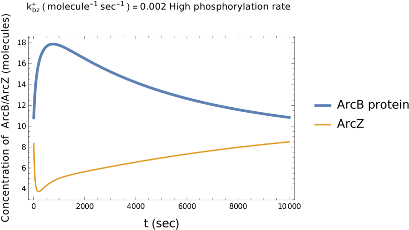
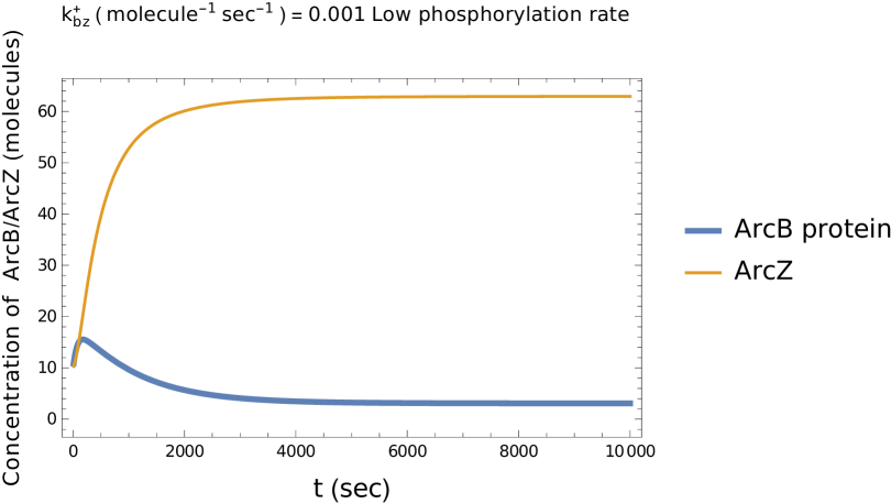
Figure 3: The time evolution of the number of ArcB and ArcZ molecules per cell for a high (panel 1) and low (panel 2) phosphorylation rate with $k_{\rm AP}=0.1\ {\rm molecule}^{-1}$ and $k_{\rm AP}=0.001\ {\rm molecule}^{-1}$, respectively. The remaining parameter values are as mentioned in table 2.

3.1.2 Role of sRNA mediated destabilisation of mRNA

The dependence of the equilibrium concentration of Z-sRNA on $k_{bz}^{+}$ can be understood by analyzing equation (12). For high phosphorylation rate, that is for a high value of $K$, one may expect $(\gamma_{bm}+K-\frac{\beta_{z}}{\gamma_{z}}G_{z}^{\rm tot}k_{bz}^{+})$ to be large positive. The concentration of Z-sRNA can be approximated as

$$[Z]\approx\frac{\gamma_{bm}}{\gamma_{z}}\beta_{z}G_{z}^{\rm tot}/(\gamma_{bm}+K-\frac{\beta_{z}}{\gamma_{z}}G_{z}^{\rm tot}k_{bz}^{+}).$$ (13)

Thus under high phosphorylation rate, Z-sRNA concentration has a low value which becomes independent of $k_{bz}^{+}$ for $k_{bz}^{+}<<(\gamma_{bm}+K)/(\frac{\beta_{z}}{\gamma_{z}}G_{z}^{\rm tot})$ (see figure (4)). However, this low concentration scenario may change drastically if the sRNA-mediated mRNA degradation rate ($k_{bz}^{+}$) is increased. With the increase in this rate, mRNA degradation increases and this increases the concentration of Z-sRNA abruptly even when the phosphorylation rate is high. Equation (12) implies that this abrupt change in concentration must happen when $(\gamma_{bm}+K-\frac{\beta_{z}}{\gamma_{z}}G_{z}^{\rm tot}k_{bz}^{+})$ changes sign with the increase in $k_{bz}^{+}$. In figure (4), we show how the concentration of Z-sRNA increases with $k_{bz}^{+}$ in case of high phosphorylation rate.

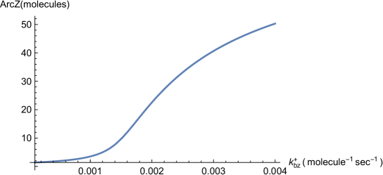
Figure 4: Number of ArcZ molecules per cell for different values of $k_{\rm bz}^{+}$ for a high phosphorylation rate, $k_{AP}=0.1\ {\rm molecule^{-1}}$. The remaining parameter values are as given in table 2.

This drastic behaviour originating from sRNA-mRNA interaction might be compared with threshold linear response seen earlier in the context of sRNA mediated mRNA degradation hwa ; hwa2 even when there was no feedback component in the regulation. In the threshold-linear response, the gene expression is completely silenced when the target transcription rate is below a threshold. Above the threshold, mRNAs code for the protein leading to a linear increase in the protein concentration with the target transcription rate. In case of strong sRNA, mRNA interaction, the transition from one gene expression regime to the other is sharp. As the interaction between sRNA and mRNA becomes weaker, the transition becomes smoother although the threshold-linear form is preserved. Figure (4) describes a similar smooth transition from a negligible sRNA expression regime to a high sRNA expression regime except for the fact that, beyond the threshold, the change in the concentration with $k^{+}_{bz}$ is not linear. This entire phenomenon is the result of the nonlinear interactions between sRNA and mRNA ( $k_{bz}^{+}$ dependent term in equation (1)) and accordingly, no drastic effect, for example, of an increase in the mRNA degradation rate can be seen on the sRNA concentration (see figure 5).

Figure 5: Number of ArcZ molecules per cell for different values of $\gamma_{bm}$ for a high phosphorylation rate, $k_{AP}=0.1\ {\rm molecule}^{-1}$. The remaining parameter values are as given in table 2.

3.2 Model II

Applying the steady-state condition on (9), (7) and (8), we have the following equation for the steady-state concentration $[Z]$.

$$\frac{\beta_{z}}{\gamma_{z}}G_{z}^{tot}-[Z]=[Z]\frac{{{K}}^{2}}{k_{z}(k_{bz}^{+}[Z]+\gamma_{bm})^{2}}$$ (14)

where, as before, ${K}=\frac{k_{z}k_{AP}{r_{bp}}r_{bm}[A]}{\gamma_{bp}}$.

Being a cubic equation in $[Z]$, equation (14) leads to three equilibrium solutions for $[Z]$ for certain parameter values. Figure (6) shows these three solutions over a range of values of $k_{bz}^{+}$. The upper most and the lower most branches of solutions are stable branches, while the intermediate branch is the unstable branch.

Figure 6: The three branches of the equilibrium solution of $[Z]$ for model II. The uppermost (dash-dotted) and the lowermost (solid) lines are the stable branches of the solution. The intermediate (dotted) line corresponds to the unstable branch of the solution. For this plot $k_{AP}=0.1\ {\rm molecule}^{-1}$. The other parameter values are as displayed in table 2 except that here $\gamma_{bm}=0.001\ {\rm sec}^{-1}$.

Since in case of model I, the phosphorylation rate and $k_{bz}^{+}$ are crucial for the threshold response of sRNA expression, we are interested to know how, for model II, these two parameters alter the threshold response behaviour and gives rise to two possible stable states (a bistable response). The steady-state behaviour, in this case, can be presented through a phase diagram in the parameter space of $k_{bz}^{+}$ and $k_{AP}$. Equation (14) can be written as

$$f([Z])=g([Z]),\ \ {\rm where}$$ (15)

$$f([Z])=\frac{\beta_{z}}{\gamma_{z}}G_{z}^{tot}-[Z]\ \ {\rm and}\ \ g([Z])=[Z]\frac{{{K}}^{2}}{k_{z}(k_{bz}^{+}[Z]+\gamma_{bm})^{2}}.$$ (16)

The bistability of $[Z]$ is found when, for a given parameter values, the linear function $f([Z])$ intersects $g([Z])$ at three different $[Z]$ values. The onset of bifurcation (bistability) happens at particular parameter values at which the straight line $f([Z])$ meets $g([Z])$ as a tangent at a particular value of $[Z]$ strogatz . Thus the onset of bifurcation can be analysed by solving equation (14) together with the condition arising from slope matching of the two curves $f([Z])$ and $g([Z])$ i.e.

$$\frac{d}{d[Z]}f([Z])=\frac{d}{d[Z]}g([Z]),$$ (17)

Solving these two equations for $k_{AP}$ and $[Z]$ for different values of $k_{bz}^{+}$ and for fixed values of other parameters, we obtain the bistable region in $k_{bz}^{+}$ and $k_{AP}$ parameter space (see figure (7)). It is apparent from the phase diagram that the threshold response that was seen in case of model I, disappears in this case. The threshold response was seen for high phosphorylation rate for which sRNA synthesis is low upto a certain value of $k_{bz}^{+}$ but increases rapidly as $k_{bz}^{+}$ increases beyond this value. This continuous variation in the value of $[Z]$ from a low to a high value is governed by a single equilibrium solution of $[Z]$ (see figure (4)). As the phase diagram in figure (7) shows, in case of model II, for high values $k_{AP}$, the low $[Z]$ state enters into the bistable region as the strength of the sRNA-mRNA interaction, $k_{bz}^{+}$, is increased.

Figure 7: The phase diagram of model II in the $k_{bz}^{+}$ -$k_{AP}$ parameter space. The parameter values are as displayed in table 2 except that here $\gamma_{bm}=0.001\ {\rm sec}^{-1}$.

3.3 Model III

For model III, bistable solutions similar to that of model II are found. As before, the steady-state solutions for $[Z]$ are found from the following equation

$$f([Z])=g([Z]),\ \ {\rm where}$$ (18)

$$f([Z])=\gamma_{z}(\gamma_{bm}+k_{bz}^{+}[Z])+k_{bz}^{+}r_{bm}\ \ {\rm and}\ \ \ g([Z])=\frac{\beta_{z}G_{z}^{\rm tot}(\gamma_{bm}+k_{bz}^{+}[Z])^{2}}{[Z](\gamma_{bm}+k_{bz}^{+}[Z]+K)}$$ (19)

The solutions for $[Z]$ as $k_{bz}^{+}$ is varied for a specific value of $k_{AP}$ is shown in figure (8).

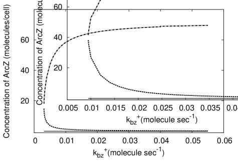
Figure 8: The three branches of the equilibrium solution of $[Z]$ for model III. The uppermost (dash-dotted) and the lowermost (solid) lines are the stable branches of the solution. The intermediate (dotted) line corresponds to the unstable branch of the solution. For this plot, $k_{AP}=0.1\ {\rm molecule}^{-1}$. The other parameter values are as displayed in table 2 except that here $\gamma_{bm}=0.001\ {\rm sec}^{-1}$.

Here also, for a given value of $k_{bz}^{+}$, there is a range of $k_{AP}$ over which bistablity in $[Z]$ is found. The phase diagram obtained upon solving (18) and the equation for slope matching ( $\frac{df([Z])}{d[Z]}=\frac{dg([Z])}{d[Z]}$) numerically, is shown in figure (9). A comparison with the phase diagrams of model II shows that model III has a much wider bistable region indicating that the co-degradation of sRNA gives rise to a more robust bistable behaviour in comparison with model II where the bistability arises due to cooperativity.

Figure 9: The phase diagram of model III in the $k_{bz}^{+}$ -$k_{AP}$ parameter space. The parameter values are as displayed in table 2 except that here $\gamma_{bm}=0.001\ {\rm sec}^{-1}$.

4 Stochastic analysis

4.1 Methodology

In our previous analysis, we have framed the time evolution equation for Z-sRNA incorporating various terms originating from transcriptional and translational regulation. The bistable response found in model II and model III can give rise to phenotypic heterogeneity in a bacterial population. The differential equation method discussed in the previous section describes the noise-free dynamics of the system and indicates that, in case of model II and model III, there are two stable equilibrium states for a cell with low and high concentration levels of sRNA. These two states are separated by an unstable state which sets a barrier for crossing over from one equilibrium state to another. In this picture, the equilibrium state of the cell is determined by the initial condition or previous history. For example, if cells in a population are in certain initial state supporting high or low expression level, all the cells in this population would continue to remain in the same state in the equilibrium also. In reality, the gene expression is inherently noisy. Due to the noise, in experiments, the signature of bistability is found through the coexistence of two subpopulations of cells with low and high expression levels kaern ; raj ; maamar . This happens due to noise driven transitions of a cell from one state to another. Due to fluctuations (noise) in gene expression, a cell in the low-expression state, for example, may cross over to the high-expression state by overcoming the barrier corresponding to the intermediate unstable state. Such bistable expression pattern of cells has been observed in synthetic networks also becskei . The primary aim of this part of the work is to study the effect of noise on the bistable response seen in model II and III. Based on the origin, the noise is categorised as (i) extrinsic and (ii) intrinsic noise swain ; elowitz . The extrinsic noise is due to gene independent fluctuations which, for example, might be due to fluctuations in the amount of RNA polymerase which itself is a gene product. The intrinsic noise, on the other hand, is due to gene specific fluctuations which might be, for example, due to random occurrences of various biochemical events associated with translation and transcription. In the past, there have been experimental studies to quantify the noise and discriminate the two mechanisms behind the origin of these two types of noise. These studies provide valuable inputs regarding the role of noise in the cell-cell variation in gene expression as well as in intracellular reactions elowitz .

In the presence of noise, the concentration levels of various components must be described probabilistically. Here, we use the Fokker-Planck equation based method to obtain the probability distributions of sRNA concentrations in various cases. The bistable response, observed using the differential equation method, leads to a bimodal probability distribution in the Fokker-Planck approach. Such bimodal distributions indicate that there are significant probabilities for a cell to be in two distinct states with distinctly different protein concentration levels. Further, this analysis allows us to find how the noise strength or the noise correlation influences the nature of the distribution. The present section is primarily devoted to general, formulation related discussions. Model specific results are derived in the following subsections.

The stochastic analysis begins with the Langevin equation which describes the time evolution of the sRNA concentration as shown in equation (9) or (10) along with additional noise terms hasty ; sayantari ; zheng . In order to simplify notations, we denote the concentration of Z-sRNA as $z$ below. Considering the presence of two different types of noise, we write below the Langevin equation with both multiplicative and additive noise

$$\frac{dz}{dt}=f(z)+g(z)\epsilon(t)+\eta(t).$$ (20)

The forms of $f(z)$ and $g(z)$ change depending on the model considered. As discussed in detail in the next subsection, for model II, the explicit forms of $f(z)$ and $g(z)$ can be obtained by separating the deterministic and the noisy parts of the first term in equation (9). In a similar way, for model III, the forms of $f(z)$ and $g(z)$ are obtained from equation (10) (see subsection (4.3)). The additive noise, denoted by $\eta(t)$, represents random fluctuations in the external environment and it is usually not directly related to the gene concerned. The multiplicative noise, $\epsilon(t)$, on the other hand, represents the intrinsic noise that originates from the randomness in various biochemical events associated with the transcription or translation. Such transcription or translation processes, for example, are regulated by the participation of various regulatory molecules whose presence or absence is somewhat random leading to random rate parameters. The effects of all such randomness are lumped together into a single multiplicative noise term $g(z)\epsilon(t)$. The multiplicative and additive noise obey Gaussian distribution with the following correlations

$$\langle\epsilon(t)\epsilon(t^{\prime})\rangle=2D_{1}\delta(t-t^{\prime}),$$ (21)

$$\langle\eta(t)\eta(t^{\prime})\rangle=2D_{2}\delta(t-t^{\prime})\ \ \ {\rm and}$$ (22)

$$\langle\eta(t)\epsilon(t^{\prime})\rangle=\langle\epsilon(t)\eta(t^{\prime})\rangle=2\lambda\sqrt{D_{1}D_{2}}\delta(t-t^{\prime}).$$ (23)

Here $D_{1}$ and $D_{2}$ denote the strength of the two types of noise $\epsilon(t)$ and $\eta(t)$, respectively. $\lambda$ denotes the correlation between the additive and the multiplicative noise. For $\lambda=0$, the two types of noise are uncorrelated. $\epsilon(t)$ and $\eta(t)$ are expected to be correlated ($\lambda\neq 0$) when these two types of noise are of same origin. $f(z)$ in equation (20) takes into account the deterministic parts in equation (9) or (10).

Beginning with this Langevin equation, one may obtain the Fokker-Planck (FP) equation following the standard procedure reichl . The FP equation describes the time evolution of the probability density $\rho(z,t)$ with $\rho(z,t)dz$ denoting the probability of having the concentration, $z$, between $z$ and $z+dz$ at time $t$. The FP equation derived from (20) is

$$\frac{d\rho}{dt}=-\frac{d}{dz}[A(z)\rho(z,t)]+\frac{d^{2}}{dz^{2}}(B(z)\rho(z,t)),$$ (24)

where

$$A(z)=f(z)+D_{1}g(z){\big{(}}\frac{d}{dz}g(z){\big{)}}+\sqrt{D_{1}D_{2}}\lambda{\big{(}}\frac{d}{dz}g(z){\big{)}},\ \ {\rm and}\ \$$ (25)

$$B(z)=D_{1}g(z)^{2}+2\lambda\sqrt{D_{1}D_{2}}g(z)+D_{2}.$$ (26)

In the steady-state, the probability distribution is independent of time ($\frac{d\rho(z,t)}{dt}=0$). The solution for the steady-state probability density is

$$\rho(z)=\frac{N}{B(z)}\exp[\int^{z}\frac{A(z^{\prime})}{B(z^{\prime})}dz^{\prime}],$$ (27)

where $N$ is the normalisation factor. $\rho(z)$ can be further simplified as

$$\rho(z)=\frac{N}{\{D_{1}g(z)^{2}+2\lambda\sqrt{D_{1}D_{2}}g(z)+D_{2}\}^{1/2}}\exp[\int^{z}dz^{\prime}\ \frac{f(z^{\prime})}{\{D_{1}g(z^{\prime})^{2}+2\lambda\sqrt{D_{1}D_{2}}g(z^{\prime})+D_{2}\}}.$$ (28)

Following this general formulation, we obtain the probability distributions for specific models below.

4.2 Model II

For model II, we proceed with equation (20) with

$$f(z)=p_{0}\frac{(z+\gamma)^{2}}{(z+\gamma)^{2}+p_{2}}-\gamma_{z}z\ \ {\rm and}\ \ g(z)=\frac{(z+\gamma)^{2}}{(z+\gamma)^{2}+p_{2}}$$ (29)

These forms of $f(z)$ and $g(z)$ are obtained by using the expressions for steady concentrations of $[AP]$, $[B_{p}]$ and $[B_{m}]$ in equation (9). We have assumed steady-state conditions, $\frac{d}{dt}[\sigma^{s}mZ]=\frac{d}{dt}[B_{m}Z]=0$ (see equations (7) and (8)) for the concentrations of mRNA-sRNA complexes, $[\sigma^{s}mZ]$ and $[B_{m}Z]$. In equation (29), $p_{0}=\beta_{z}G_{z}^{\rm tot}$, $p_{2}=\frac{K^{2}}{k_{z}{k_{bz}^{+}}^{2}}$ and $\gamma=\frac{\gamma_{bm}}{k_{bz}^{+}}$. The form of $g(z)$ in (29) can be understood from the origin of the multiplicative noise. Here we assume that various biochemical events associated with transcription makes $p_{0}$, effectively, noisy. Thus a noise in the form $p_{0}\rightarrow p_{0}+\epsilon(t)$ leads to the above expression of $g(z)$. Substituting these forms of $f(z)$ and $g(z)$ in equation (28), we find the probability distribution numerically for different cases such as only additive noise, additive and multiplicative noise without correlation ($\lambda=0$) and finally, additive and multiplicative noise with correlation ($\lambda\neq 0$).

The probability distributions for the concentration, $z$, are bimodal with two peaks near high and low $z$ values. As shown in figure (10), in case of additive noise, the peak in the distribution at low $z$ value is much smaller in comparison to the peak at high $z$ value. This indicates that the high z state is more favorable in comparison to low z states. This scenario, however, changes since with the increase in the noise strength and the correlation between the multiplicative and additive noise, the peak of the distribution at low z value becomes significantly more prominent. This implies that the cells with low concentration of sRNA are more probable as the strength of the multiplicative noise or the correlation between the two types of noise is increased. Further, the probability distributions become broader as the strength of the noise and the correlation between the additive and multiplicative noise increases. As we show below, this feature is not observed for model III. Such broadening of distributions indicates that the noise strength or the noise correlation might give rise to noise driven heterogeneity in the microbial population.

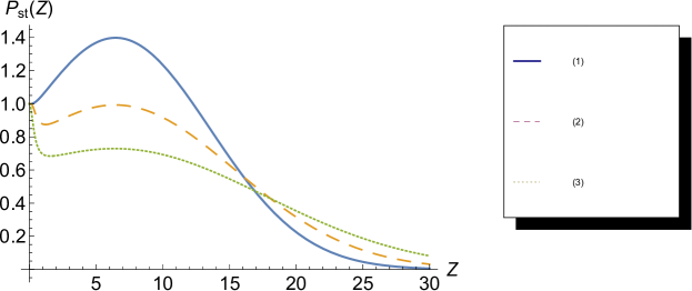
(a) $p_{0}=0.13$

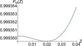
(b) $p_{0}=0.13$

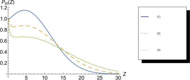
(c) $p_{0}=0.09$

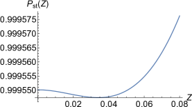
(d) $p_{0}=0.09$

Figure 10: Probability distributions for model II with (1) additive noise ($D_{2}=1$) (2) additive and multiplicative noise without correlation ($D_{2}=1$, $D_{1}=0.6$ and $\lambda=0$) (3) additive and multiplicative noise with correlations ($D_{2}=1$, $D_{1}=0.6$ and $\lambda=0.6$) are plotted. Other parameter values are $\gamma=0.005$, $p_{2}=0.2$ and $\gamma_{z}=0.02$. Since the peak in the probability distributions near low $z$ is not seen in figures (a) and (c), we have shown in figures (b) and (d) the respective distributions near the low concentration region with appropriate zooming.

4.3 Model III

For model III,

$$f(z)=\frac{p_{0}(z+\gamma)}{(z+p_{1})}-r_{bm}\frac{z}{z+\gamma}-\gamma_{z}z.$$ (30)

These forms are again obtained by using the expressions for steady concentrations of $[AP]$, $[B_{p}]$ and $[B_{m}]$ in equation (10). For the concentrations of mRNA-sRNA complex, $[\sigma^{s}mZ]$, we have assumed a steady-state condition, $\frac{d}{dt}[\sigma^{s}mZ]=0$ (see equation (8)). In (30), $p_{0}=\beta_{z}G^{z}_{\rm tot}$, $\gamma=\frac{\gamma_{bm}}{k_{bz}^{+}}$ and $p_{1}=\gamma+\frac{K}{k_{bz}^{+}}$. As before, the form of $g(z)$ can be understood from the origin of the multiplicative noise. Here, we consider two possibilities for the multiplicative noise. If the fluctuations in various rate parameters effectively lead to a noisy $p_{0}$, we may choose $p_{0}\rightarrow p_{0}+\epsilon(t)$ such that $g(z)=\frac{z+\gamma}{z+p_{1}}$. The other possibility that we consider here is an effective fluctuation or noise in $r_{bm}$ as $r_{bm}\rightarrow r_{bm}+\epsilon(t)$ for which $g(z)=-\frac{z}{z+\gamma}$.

Using these forms of $f(z)$ and $g(z)$, we obtain stationary distributions for only additive noise, both additive and multiplicative noise without correlation ($\lambda=0$) and additive and multiplicative noise with correlation ($\lambda\neq 0$.). The distributions for $g(z)=\frac{z+\gamma}{z+p_{1}}$ are displayed in figure (11).

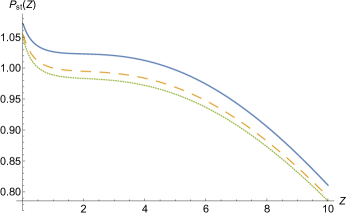
(a) $p_{0}=0.26$

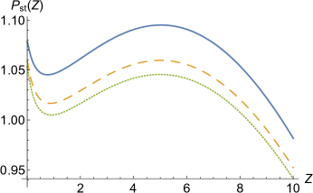
(b) $p_{0}=0.28$

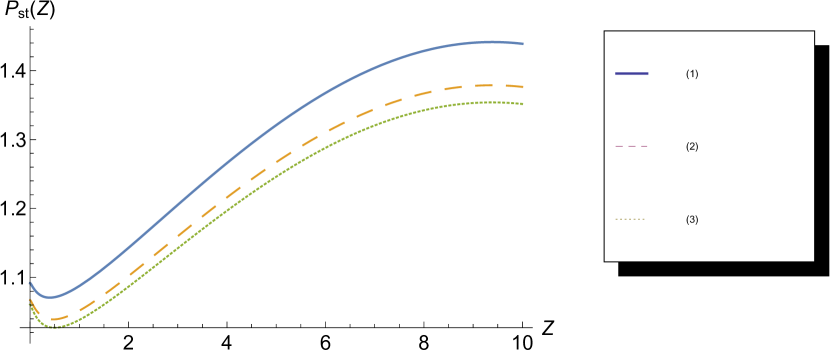
(c) $p_{0}=0.32$

Figure 11: Probability distributions for model III with $g(z)=\frac{z+\gamma}{z+p_{1}}$ and with (1) additive noise ($D_{2}=1$, $D_{1}=0$ and $\lambda=0$) (2) additive and multiplicative noise without correlation ($D_{2}=1$, $D_{1}=0.03$ and $\lambda=0$) (3) additive and multiplicative noise with correlations ($D_{2}=1$, $D_{1}=0.03$ and $\lambda=0.05$) are plotted. Other parameter values are $\gamma=0.01$, $p_{1}=0.2$, $r_{bm}=0.22$ and $\gamma_{z}=0.01$.

The figure shows the role of the synthesis rate of sRNA, i.e. $p_{0}$, on the probability distributions under different types of noise. The probability distribution for $p_{0}=0.28$ is prominently bimodal with two peaks at low and high $z$ values. For synthesis rates lower than $p_{0}=0.28$, the peak at large $z$ becomes less prominent indicating that the low sRNA expression state is more favourable. For high synthesis rate, the peak at high $z$ becomes more prominent showing a tendency of having higher concentration of sRNA. An additional figure presented in appendix (D) (see figure (12) in the appendix) shows that, for a given synthesis rate, as the noise strength or the correlation between the two types of noise increases, the peak in the probability distribution near the low $z$ value becomes more prominent indicating that the cells are more likely to be in the low sRNA expression state as compared to the high expression state. Figure (13) in appendix (D) shows the probability distributions for $g(z)=-\frac{z}{z+\gamma}$ for different synthesis rates of Z-sRNA. The role of correlation ($\lambda$) between the two different types of noise appears to be different from the previous case (Figure (11)).

Finally, for all these cases with different noise strength and noise correlations, no trend of broadening of the probability distribution is found. This feature is in sharp contrast to model II, where the probability distribution broadens with the increase in the noise strength and noise correlations.

5 Discussion

In this paper, we have shown that subtle changes in the architecture of a minimal network involving transcriptional and translational regulation can bring in drastic changes in the end result. This analysis is done on an Arc protein network responsible for regulation in the synthesis of $\sigma^{s}$ in E.coli under stress due to oxygen and energy availability. We are particularly interested in a network motif that uses dual strategies involving both transcriptional and translational regulation. The histidine sensor kinase ArcB phosphorylates a protein regulator ArcA which represses transcription of ArcZ sRNA. ArcZ sRNA, through a feedback mechanism, destabilises ArcB mRNA and thus autoregulates its own synthesis. Starting with this network, we have considered three different scenarios. While in the first case (Model I), the sRNA synthesis is repressed by a single repressor molecule of phosphorylated ArcA, in the second case (Model II), the synthesis of sRNA is repressed by a homodimer of the repressor molecule. In the third case (Model III), we introduce co-degradation of the sRNA along with the target mRNA. In all these cases, the networks show ultrasensitive response in the sRNA concentration. We show that while in case of Model I, the concentration of sRNA shows a monostable response with a threshold behaviour, in case of Model II and Model III, the sRNA concentration shows a bistable response. Intuitively, as per the network in figure (1), for high phosphorylation rates, the synthesis of sRNA is tightly repressed. However, as the sRNA mediated mRNA degradation rate is enhanced, the sRNA concentration increases drastically beyond a threshold value of this rate. In general, such threshold behavior is believed to be necessary for controlling cellular response which might be expensive in terms of energy or nutrient. Further, through this mechanism, an immediate response to transient signals can also be avoided. The threshold response, however, disappears completely in case of model II and III. In these cases, at a high phosphorylation rate and for low rate of sRNA mediated mRNA degradation, the sRNA concentration is low. However, as the sRNA mediated mRNA degradation rate is increased, the sRNA concentration shows a bistable response with high and low values of the concentration. Further, the phase diagram, in terms of the phosphorylation rate and the sRNA mediated mRNA degradation rate, obtained for model II and model III shows that the bistable response of model III is more robust with a much wider bistable region as compared to model II.

The noise in gene expression is known to give rise to phenotypic transitions from one state to another maamar . For example, in case of bistability, there might be large fluctuations (noise) due to which a cell switches from one stable state to another upon crossing the barrier caused by the intermediate unstable state. Such noise driven transitions may lead to two distinct subpopulations in a bacterial colony and, thereby, enhance the survival probability of bacteria under stress since all the cells do not suffer the same fate. In the next part, we have studied the influence of noise on the bistable response found in the deterministic analysis of model II and model III. Broadly, the gene expression is affected by two types of noise (i) extrinsic and (ii) intrinsic noise. While the extrinsic noise is due to the perturbation in the external environment unrelated to the gene(s) involved, the intrinsic noise arises, for example, due to various biochemical processes associated with the translation or transcription of the gene involved. As an example of the latter, although transcription is often considered as a single biochemical process, it is actually preceded by a sequence of biochemical events whose random occurrences might effectively introduce noise in the transcription rate. Considering that the intrinsic noise in a specific cellular component can be a source of extrinsic noise for other cellular components, we have proceeded with a general formulation by including both extrinsic and intrinsic noise terms. The extrinsic and intrinsic noise are incorporated through additive and multiplicative noise terms in the Langevin equations appropriate for model II and model III. Beginning with such Langevin equations, we obtain the Fokker-Planck equations which describe the time evolution of the probability distribution of sRNA concentration for the two models. The steady-state probability distributions for both models are found to be bimodal with two peaks at low and high sRNA concentrations. The peaks correspond to the high and low expression stable states found in the deterministic analysis of model II and III showing bistability. The stochastic formulation allows us to study how the probability distributions especially the peaks in the distributions change as the noise strength and the noise correlation are altered. In general, the stochastic analysis shows that as the noise strength or the correlation between the two types of noise is increased, the peak in the probability distribution near the low sRNA concentration becomes more pronounced indicating an increased possibility of finding cells with low sRNA concentration in an ensemble of cells. We also observe an interesting feature that unlike model III, model II shows a broadening of the probability distributions with the noise strength or the noise correlation. Such broadening of the probability distribution hints towards an increased population heterogeneity in the bacterial colony.

Although the work is motivated from a specific network motif relevant for bacterial stress response, various models discussed here might, in general, have broad implications due to their drastically different outcomes. Further, the models and the results might be of relevance in the context of designing synthetic networks leading to artificial control.

Appendix A Reaction Scheme

Different biochemical reactions that we have considered are

$$ArcA+ArcB\rightarrow ArcA\mbox{-}ArcB\ {\rm(ArcA\ and\ ArcB\ complex\ formation)}$$ (31)

$$ArcA\mbox{-}ArcB\rightarrow ArcA\mbox{-}P+ArcB\ {\rm(Phosphorylation\ of\ ArcA)}$$ (32)

$$ArcA\mbox{-}ArcB\rightarrow ArcA+ArcB\ {\rm(ArcA\mbox{-}ArcB\ complex\ dissociation)}$$ (33)

$$ArcA\mbox{-}P\rightarrow ArcA+P$$ (34)

$$ArcA\mbox{-}P+G_{\sigma}\rightarrow\overline{G_{\sigma}}\ {\rm(transcriptional\ repression\ byArcA\mbox{-}P)}$$ (35)

$$\overline{G_{\sigma}}\rightarrow G_{\sigma}+ArcA\mbox{-}P$$ (36)

$$G_{\sigma}\rightarrow\sigma^{s}m+G_{\sigma}$$ (37)

$$ArcA\mbox{-}P+G_{z}\rightarrow\overline{G_{z}}\ {\rm(transcriptional\ repression\ byArcA\mbox{-}P)}$$ (38)

$$\overline{G_{z}}\rightarrow G_{z}+ArcA\mbox{-}P$$ (39)

$$G_{z}\rightarrow ArcZ+G_{z}\ {\rm(synthesis\ of\ small\ regulatory\ RNA,\ ArcZ)}$$ (40)

$$ArcZ+\sigma^{s}m\rightarrow\sigma^{s}m\mbox{-}ArcZ\ {\rm(binding\ of\ ArcZ\ and\ \sigma^{s}\ mRNA)}$$ (41)

$$\sigma^{s}m\mbox{-}ArcZ\rightarrow\sigma^{s}m+ArcZ$$ (42)

$$\sigma^{s}m\mbox{-}ArcZ\rightarrow\sigma^{s}+\sigma^{s}m\mbox{-}ArcZ\ {\rm(synthesis\ of\ \sigma^{s})}$$ (43)

$$ArcZ+ArcBm\rightarrow ArcBm\mbox{-}ArcZ\ {\rm(complex\ of\ ArcB\ and\ ArcZ)}$$ (44)

$$ArcBm\mbox{-}ArcZ\rightarrow ArcZ\ {\rm(ArcZ\ mediated\ degradation\ of\ ArcB\ mRNA)}$$ (45)

$$\sigma^{s}m\rightarrow\emptyset\ ({\rm degradation\ of\ \sigma^{s}\ mRNA})$$ (46)

$$\emptyset\rightarrow ArcA\ {\rm(supply\ of\ ArcA)}$$ (47)

$$\emptyset\rightarrow ArcBm\ {\rm(supply\ of\ ArcB\ mRNA)}$$ (48)

$$\emptyset\rightarrow ArcB\ {\rm(synthesis\ of\ ArcB\ protein)}$$ (49)

$$ArcA\rightarrow\emptyset\ {\rm(degradation\ of\ ArcA\ protein)}$$ (50)

$$ArcBm\rightarrow\emptyset\ {\rm(degradation\ of\ ArcB\ mRNA)}$$ (51)

$$ArcB\rightarrow\emptyset\ {\rm(degradation\ of\ ArcB\ protein)}$$ (52)

$$ArcZ\rightarrow\emptyset\ {\rm(degradation\ of\ ArcZ)}$$ (53)

Here $\sigma^{s}m$, ArcBm, represent $\sigma^{s}$ mRNA, ArcB mRNA, respectively. ArcZ, ArcA represent the small regulatory RNA ArcZ and ArcA protein, respectively. Further, ArcA-ArcB, ArcB-ArcZ and ArcA-P represent ArcA-ArcB complex, ArcB-ArcZ complex, a phosphorylated ArcA molecule, respectively. $G_{\sigma}$ and $G_{z}$ represent average number of $\sigma^{s}$ and arcz genes, respectively. $\overline{G_{\sigma}}$ and $\overline{G_{z}}$ represent the inactive states of the genes upon the action of the transcriptional repressor ArcA-P. $\sigma^{s}m\mbox{-}$ArcZ and ArcBm-ArcZ represent the bound complexes of $\sigma^{s}$ mRNA and ArcZ, ArcB mRNA and ArcZ, respectively.

Appendix B Phosphorylation of ArcA

$$ArcA+ArcB\underset{k_{c}^{-}}{\stackrel{{\scriptstyle k_{c}^{+}}}{{\rightleftharpoons}}}ArcAB{\stackrel{{\scriptstyle k_{p}^{+}}}{{\rightarrow}}}ArcAP+ArcB$$ (54)

$$ArcAP{\stackrel{{\scriptstyle k_{p}^{-}}}{{\rightarrow}}}ArcA+P$$ (55)

These phosphorylation reactions are described by the following differential equations

$$\frac{d[A]}{dt}=-k_{c}^{+}[A][B_{p}]+k_{c}^{-}[AB_{p}]+k_{p}^{-}[AP]+r_{A}-\gamma_{A}[A]$$ (56)

$$\frac{d[AP]}{dt}=k_{p}^{+}[AB_{p}]-k_{p}^{-}[AP]$$ (57)

$$\frac{d[AB_{p}]}{dt}=k_{c}^{+}[A][B_{p}]-k_{c}^{-}[AB_{p}]-k_{p}^{+}[AB_{p}].$$ (58)

As was mentioned in the main text, $[A]$, $[AP]$, $[AB_{p}]$ denote the concentrations of ArcA, phosphorylated ArcA and ArcA, ArcB protein complexes, respectively. Possible nontrivial equilibrium solutions of (56), (57) and (58) are

$$[A]=\frac{r_{A}}{\gamma_{A}},\ \ [AP]=\frac{k_{p}^{+}}{k_{p}^{-}}[AB_{p}],$$ (59)

$$[AB_{p}]=\frac{k_{c}^{+}}{k_{c}^{-}+k_{p}^{+}}[A][B_{p}].$$ (60)

Combining equations (59) and (60), we find

$$[AP]=\frac{k_{p}^{+}}{k_{p}^{-}}\frac{k_{c}^{+}}{k_{c}^{-}+k_{p}^{+}}[A][B_{p}]=\frac{k_{p}k_{c}}{1+k_{p}^{+}/k_{c}^{-}}[A][B_{p}]=k_{AP}[A][B_{p}]$$ (61)

where $k_{p}=\frac{k_{p}^{+}}{k_{p}^{-}}$, $k_{c}=\frac{k_{c}^{+}}{k_{c}^{-}}$ and $k_{AP}=\frac{k_{p}k_{c}}{1+k_{p}^{+}/k_{c}^{-}}$.

For all calculations, we have assumed a fixed value for the steady concentration of ArcA.

Appendix C Repressor activity of phosphorylated ArcA

Let $G_{\sigma}$, $\bar{G_{\sigma}}$ represent the average number of the repressor-free and repressor-bound forms of the $\sigma^{s}$ gene, respectively. Similar meaning is implied here for $G_{z}$ and $\bar{G_{z}}$ for the ArcZ expressing gene. Let us assume

$$G_{\sigma}+\bar{G_{\sigma}}=G_{\sigma}^{\rm tot}$$ (62)

$$G_{z}+\bar{G_{z}}=G_{z}^{\rm tot}.$$ (63)

With the reaction scheme as

$$G_{\sigma}+ArcAP\underset{k_{\sigma}^{-}}{\stackrel{{\scriptstyle k_{\sigma}^{+}}}{{\rightleftharpoons}}}\bar{G_{\sigma}}\ \ {\rm and}\ \ G_{z}+ArcAP\underset{k_{z}^{-}}{\stackrel{{\scriptstyle k_{z}^{+}}}{{\rightleftharpoons}}}\bar{G_{z}},$$ (64)

the time evolution of these average numbers can be described through equations similar to

$$\frac{dG_{\sigma}}{dt}=k_{\sigma}^{-}\bar{G_{\sigma}}-k_{\sigma}^{+}G_{\sigma}[AP].$$ (65)

Employing equilibrium condition on (65) and using (62), we have

$$G_{\sigma}=\frac{G_{\sigma}^{\rm tot}}{1+k_{\sigma}[AP]}\ \ {\rm and}\ \ G_{z}=\frac{G_{z}^{\rm tot}}{1+k_{z}[AP]},$$ (66)

where $k_{\sigma}=\frac{k_{\sigma}^{+}}{k_{\sigma}^{-}}$ and $k_{z}=\frac{k_{z}^{+}}{k_{z}^{-}}$. There are other loss and gain terms in equation (57) due to the repression activities of [AP]. However, these terms will not contribute once the equilibrium conditions as used in equation (65) are imposed.

Appendix D The role of noise on the peaks in the distribution

Figure (12) shows how, for a given Z-sRNA synthesis rate, the noise strength and noise correlation influence the probability distributions for model III with $g(z)=\frac{z+\gamma}{z+p_{1}}$.

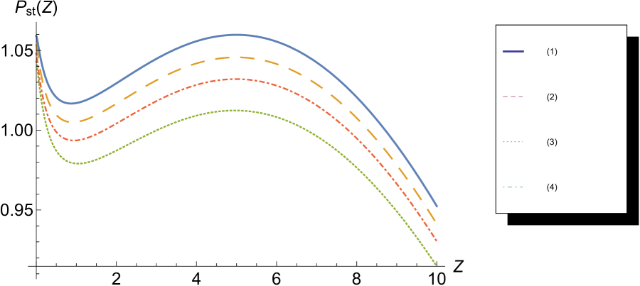
Figure 12: Probability distributions for model III with $g(z)=\frac{z+\gamma}{z+p_{1}}$ and with both additive and multiplicative noise (1) $D_{1}=0.03$, $D_{2}=1$ and $\lambda=0$ (2) $D_{1}=0.03$, $D_{2}=1$ and $\lambda=0.05$ (3) $D_{1}=0.07$ $D_{2}=1$ and $\lambda=0.05$ and (4) $D_{1}=0.03$ $D_{2}=1$ and $\lambda=0.1$. The other parameter values for all the curves are $p_{0}=0.28$, $\gamma=0.01$, $p_{1}=0.2$ $r_{bm}=0.22$ and $\gamma_{z}=0.01$.

Figure (13) shows the probability distributions for model III with $g(z)=-\frac{z}{z+\gamma}$ for different synthesis rate of Z-sRNA.

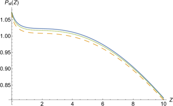
(a) $p_{0}=0.26$

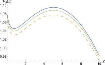
(b) $p_{0}=0.28$

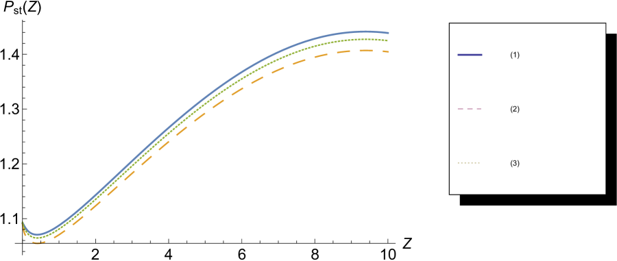
(c) $p_{0}=0.32$

Figure 13: Probability distributions for model III with $g(z)=-\frac{z}{z+\gamma}$ and with (1) additive noise ($D_{2}=1$, $D_{1}=0$ and $\lambda=0$) (2) additive and multiplicative noise without correlation with ($D_{2}=1$, $D_{1}=0.03$ and $\lambda=0$) (3) additive and multiplicative noise with correlations with ($D_{2}=1$, $D_{1}=0.03$ and $\lambda=0.05$) are plotted. These plots are obtained with $g(z)=-\frac{z}{z+\gamma}$. Other parameter values are $\gamma=0.01$, $p_{1}=0.2$, $r_{bm}=0.22$ and $\gamma_{z}=0.01$.

References

- (1) U. Alon, Introduction to Systems Biology (Chapman and Hall/CRC, London, 2006).
- (2) S. Gottesman, Trends Genet 21 399 (2005).
- (3) E. Mass and S Gottesman, Proc. Natl. Acad. Sci. 99, 4620 (2002).
- (4) N. Majdalani, S. Chen, J. Murrow, K. St John and S. Gottesman, Mol. Microbiol. 39, 1382 (2001).
- (5) K. Papenfort K and C. K. Vanderpool, FEMS Microbiol. Rev. 39, 362-378 (2015).
- (6) S. Mangan and U. Alon U, Proc. Natl. Acad. Sci. 100, 11980 (2003).
- (7) N. Rosenfeld, M. B. Elowitz, U. Alon, J. Mol. Biol. 323, 785 (2002).
- (8) S. S. Shen-orr, R. Milo, S. Mangan and U. Alon, Nat. Genet. 31, 64 (2002).
- (9) B. Ghosh, R. Karmakar and I. Bose, Phys. Biol. 2, 36 (2005).
- (10) E. Levine and T. Hwa, Curr. Opinion in Microbiol. 11, 574 (2008).
- (11) E. Levine, Z. Zhang, T. Kuhlman and T. Hwa, PLoS Biol. 5 e229 (2007).
- (12) A. Arkin, J. Ross and H.H. McAdams, Genetics 149, 1633 (1998).
- (13) O. Kobiler, A. Rokney, N. Friedman, D.L. Court, J. Stavans, A.B. Oppenheim, Proc. Natl. Acad. Sci. USA 102, 4470 (2005).
- (14) B. Novak and J.J. Tyson, J. Cell Sci. 106, 1153 (1993).
- (15) W. Sha, J. Moore, K. Chen, A.D. Lassaletta, C.S. Yi, J.J. Tyson and J.C. Sible, Proc.Natl. Acad. Sci. USA 100 975 (2003).
- (16) E.H. Davidson, D.R. McClay and L. Hood, Proc. Natl. Acad. Sci. USA 100, 1475 (2003).
- (17) A. Tiwari, J. Christian J. Ray, J. Narula, O. A. Igoshin, Mathematical Biosciences 231, 76 (2011).
- (18) E. Klauck and R. Hengge, controlling networks in Escherichia coli. in Bacterial Regulatory Networks (ed. A. Filloux), Horizon Scientific Press, Norwich, UK, pp. 1-25, 2012.
- (19) P. Mandin and S. Gottesman, EMBO J 29, 3094 (2010).
- (20) F. Mika and R. Hengge, Genes Dev. 19, 2770 (2005).
- (21) A. Toro-Roman, T. R. Mack and A. M. Stock J. Mol. Biol. 349 , 11 (2013).
- (22) R. Karmakar and I. Bose, Phys. Biol. 4, 29 (2007).
- (23) J. -W. Veening, W. K. Smits and O. P. Kuipers, Annu. Rev. Microbiol. 62, 193 (2008).
- (24) Y. Shimoni, G. Friedlander, G. Hetzroni, G. Niv, S. Altuvia, O. Biham and H. Margalit, Mol. Syst. Biol. 3, 128 (2007).
- (25) Miller CA and Beard DA 2008 Biophys. J. 96 2183.
- (26) S. H. Strogatz, Nonlinear Dynamics and Chaos (Westview Press, Colorado, USA, 2015).
- (27) M. Kaern, T. C. Elston, W. J. Blake, J. J. Collins, Nat Rev Genet. 6, 451 (2005).
- (28) A. Raj A and A. van Oudenaarden, Cell 135, 216 (2008).
- (29) H. Maamar, A. Raj and D. Dubnau, Science 317, 526 (2007).
- (30) A. Becskei, B. Seraphin and L. Serrano, EMBO J. 20, 2528 (2001).
- (31) P. S. Swain, M. B. Elowitz and E. D. Siggia, PNAS 99, 12795 (2002).
- (32) M. B. Elowitz, A. J. Levine and E. D. Siggia and P. S. Swain, Science 297, 1183 (2002).
- (33) J. Hasty, J. Pradines, M. Dolnik, and J. J. Collins, PNAS 97, 2075 (2000).
- (34) S. Ghosh, S. Banerjee and I. Bose, Euro. Phys. J. E 35, 1 (2011).
- (35) X.-D. Zheng, X.-Q. Yang, Y. Ta, PLoS One 6, e17104 (2011).
- (36) L. A. Reichl 2009 Modern Course in Statistical Physics (Germany: Wiley-VCH).