Single-particle potential of the $\Lambda$ hyperon in nuclear matter with chiral effective field theory NLO interactions including effects of $YNN$ three-baryon interactions

Abstract

Adopting hyperon-nucleon and hyperon-nucleon-nucleon interactions parametrized in chiral effective field theory, single-particle potentials of the $\Lambda$ and $\Sigma$ hyperons are evaluated in symmetric nuclear matter and in pure neutron matter within the framework of lowest order Bruckner theory. The chiral NLO interaction bears strong $\Lambda$N-$\Sigma$N coupling. Although the $\Lambda$ potential is repulsive if the coupling is switched off, the $\Lambda$N-$\Sigma$N correlation brings about the attraction consistent with empirical data. The $\Sigma$ potential is repulsive, which is also consistent with empirical information. The interesting result is that the $\Lambda$ potential becomes shallower beyond normal density. This provides the possibility to solve the hyperon puzzle without introducing ad hoc assumptions. The effects of the $\Lambda$NN-$\Lambda$NN and $\Lambda$NN-$\Sigma$NN three-baryon forces are considered. These three-baryon forces are first reduced to normal-ordered effective two-baryon interactions in nuclear matter and then incorporated in the $G$-matrix equation. The repulsion from the $\Lambda$NN-$\Lambda$NN interaction is of the order of 5 MeV at the normal density, and becomes larger with increasing the density. The effects of the $\Lambda$NN-$\Sigma$NN coupling compensate the repulsion at normal density. The net effect of the three-baryon interactions to the $\Lambda$ single-particle potential is repulsive at higher densities.

I Introduction

It is a fundamental problem to understand hyperon properties in the hadronic medium based on underlying baryon-baryon interactions. Despite the scarceness of hyperon-nucleon (YN) scattering data, various YN potential models have been developed by several groups NIJM ; NSC97 ; NIJ89 ; JUE05 ; KN07 . The empirical data of $\Lambda$ hyper-nuclei have suggested that the depth of the $\Lambda$ single-particle (s.p) potential in the nuclear medium is about 30 MeV MOT88 ; HAS06 . Most of the YN potentials account for the $\Lambda$-nucleus attractive interaction of this order, for example, in the framework of Brueckner theory YB90 ; SCH98 ; KOH00 ; VID00 . Calculations for neutron-star matter at higher densities with those interactions have shown that the $\Lambda$ hyperons become energetically favored to bypass the increasing neutron Fermi energy at $2\sim 3$ $\rho_{0}$, where $\rho_{0}=\frac{2k_{F}^{3}}{3}=0.166$ fm^-3 with the Fermi momentum $k_{F}=1.35$ fm^-1 is referred to as normal density. Beyond the onset of the $\Lambda$ emergence, the equation of state (EOS) of high-density nuclear matter naturally becomes soft. Such an EOS is difficult to explain even the standard neutron-star mass of $1.4$ solar mass ($1.4M_{\odot}$) NIS01 ; SCH06 . Recently, the situation has become more serious, after neutron stars with a mass of $2M_{\odot}$ were observed DEM10 ; ANT13 . The problem is called hyperon puzzle. It is necessary to advance the study of the interaction between the $\Lambda$ hyperon and the nucleons in the nuclear medium.

In the non-strangeness sector, the potentials derived in the framework of chiral effective field theory (ChEFT) MACH ; EHM09 have been widely employed in recent ab initio calculations of properties of atomic nuclei on the basis of nucleon-nucleon interaction. In addition to their comparable accuracy in describing nucleon-nucleon (NN) scattering data with other modern NN potentials, three-nucleon forces (3NFs) are introduced systematically and consistently with the NN sector. Baryon-baryon interactions in the strangeness sector have also been developed, although the experimental data are still limited. The parameterization of the YN potential in the lowest order of the chiral expansion was given by Polinder et al. POL06 . The extension to the next-to-leading order (NLO) was achieved by Haidenbauer et al. HAID13 . Pion-exchange YNN three-baryon forces (3BFs) were recently derived by Petschauer et al. PET16 .

In this article, $\Lambda$ and $\Sigma$ single-particle (s.p.) potentials are investigated, in the framework of lowest-order Brueckner theory (LOBT), in symmetric nuclear matter (SNM) and in pure neutron matter (PNM), using the ChEFT NLO interactions. The density-dependence of the $\Lambda$ s.p. potential in pure neutron matter is relevant to the role of strangeness in neutron star matter. Because ChEFT is low-momentum effective theory with the cutoff scale of about 500 MeV, it is not applicable beyond the density of the $2\sim 2.5\rho_{0}$. Nevertheless, it is worth to investigate properties of the $\Lambda$ hyperon in nuclear matter predicted by the microscopic ChEFT YN interactions below the limit as the basis towards the higher densities.

3NFs are indispensable to properly describe the saturation properties of nuclear matter. Therefore, it is important to estimate the effects of YNN 3BFs for hyperon properties in the nuclear medium. The advantage of ChEFT is that the 3BFs are systematically introduced. In this article, two-pion exchange $\Lambda$NN-$\Lambda$NN and $\Lambda$NN-$\Sigma$NN 3BFs are considered, following Petschauer et al. PET16 . The contributions of the 3BFs are evaluated by introducing density-dependent effective two-body YN interactions by integrating one nucleon degrees of freedom in the medium. The procedure may be referred to as normal-ordered prescription in the medium.

Hyperon properties calculated by the ChEFT interactions have been reported by Haidenbauer and Meißner HM15 and by Petschauer et al. EPJ16 . The recent publication by Haidenbauer et al. HMKW17 discusses the implication of the ChEFT interactions to the hyperon puzzle. The present article presents the results from independent calculations, which are qualitatively similar to the preceding calculations as it should because the same ChEFT hyperon-nucleon interactions are employed. The treatment of the 3BFs is improved to use general expressions for the off-shell components. The effects of the $\Lambda$NN-$\Sigma$NN are taken into account, which have not been considered before.

In section II, $\Lambda$ and $\Sigma$ LOBT s.p. potentials are evaluated at several densities first in SNM and next in PNM, using the NLO YN interactions only. The depth of the $\Lambda$ potential at the normal density is seen to be consistent with the empirical value. Salient features of the results are discussed. The outline of evaluating the normal-ordered YN interactions from the 3BFs is given in Sec. III. The $\Lambda$NN 3BF is included first, and then the influence of the $\Lambda$NN-$\Sigma$NN coupling interactions is incorporated. Explicit expressions of the normal-ordered YN interactions are presented in Appendix. The numerical results of the 3BF contributions both in SNM and PNM are shown in Sec. IV. Summary follows in Sec. V.

II Hyperon properties with NLO YN interactions

II.1 symmetric nuclear matter

Hyperon-nucleon interactions derived within ChEFT are not soft enough to be directly used in tha mean field description or perturbative method especially for the $\Lambda$N-$\Sigma$N coupling. It is necessary to introduce some effective interactions appropriate to lower-energy scale. The G-matrix equation in conventional Brueckner theory takes care of in-medium correlations to treat short-range repulsive part, and medium effects such as Pauli blocking as well as dispersion effects. The Brueckner self-consistency for the single-particle potentials amounts to including a certain set of higher-order diagrams.

Because the lowest-order Bruckner calculations have been extensively carried out in the literature YB90 ; SCH98 ; KOH00 ; VID00 , it is sufficient to note some comments for the present application as follows. 1) The continuous choice is used for the intermediate spectra. An effective mass approximation is not used, but s.p. energies are interpolated from the values at the mesh points. 2) The angle-average approximation is introduced for the Pauli operator in the numerator and the energies in the denominator of the propagator. 3) Partial waves up to the total angular momentum $J=6$ are included.

Before carrying out G-matrix calculations for hyperons, it is necessary to prepare nucleon single-practice energies, which are needed for the propagator in the G-matrix equation. In the present calculations, the nuclear matter properties MK13 obtained with the potential parametrized at the N³LO level by the Bochum-Bonn-Jülich group EGM05 are used, which include the effects of the leading-order 3NF as the density-dependent effective interactions by folding the third nucleon degrees of freedom. The components of the 3NF which is determined by the coupling constants fixed in the NN sector provide strong repulsion. This repulsion is decisively important to account for nuclear saturation properties, because the minimum of the saturation curve obtained by any realistic NN interaction locates at considerably higher densities than the empirical one. The coupling constants in the one-pion exchange contact and three-nucleon contact terms, respectively, are tuned to reasonably reproduce a saturation curve as $c_{D}=-2.5$ and $c_{E}=0.25$ for the case of the cutoff $\Lambda=550$ MeV MK13 .

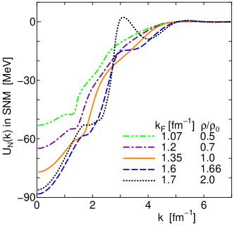
Figure 1: Nucleon s.p. potentials as a function of the nucleon momentum $k$ obtained from the LOBT calculations in SNM with the ChEFT NN potential EGM05 of the cutoff $\Lambda=550$ MeV, including the effects from the 3BF. These potentials are used for the propagator in the YN $G$-matrix equation.

The s.p. potential at the large momentum, typically $k>3$ fm^-1, starts to show oscillation as an artifact of the cutoff, when the Fermi momentum $k_{F}$ becomes large. This behavior makes it difficult to numerically obtain a Brueckner self-consistent solution. In the present calculations, a cutoff regularization in the form of $e^{-(k^{2}/(2\Lambda^{2}))^{3}}$ is applied to the single particle potential used in the $G$-matrix equation. It has been checked that the s.p. potential in the lower momentum region, $k<2$ fm^-1, has scarcely been altered by this procedure. The same prescription is applied also for the hyperon s.p. potentials. The momentum dependence of the nucleon s.p. potential with the above regularization is shown in Fig. 1 for SNM and in Fig. 2 for PNM. The nucleon s.p. potential does not become monotonically deeper as the density becomes larger because of the repulsive contribution of the 3NFs.

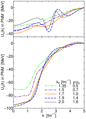
Figure 2: Same as Fig. 1, but for neutron and proton s.p. potentials in PNM.

Calculated results for the $\Lambda$ and $\Sigma$ s.p. potentials in SNM with the chiral NLO YN potentials HAID13 are shown in Fig. 3 for the real part and in Fig. 4 for the imaginary part, for the four values of the Fermi momentum; $k_{F}=1.07$, 1.35, 1.6 and 1.7 fm^-1. The corresponding densities of nuclear matter are $0.50\rho_{0}$, $\rho_{0}$, $1.66\rho_{0}$, and $2.0\rho_{0}$, respectively. Solid curves represent the results of the calculation in which the $\Lambda$N-$\Sigma$N coupling is normally included. The dotted curves are the potential after the regularization factor $e^{-(k^{2}/(2\Lambda^{2}))^{3}}$ is multiplied, which is employed in the denominator of the propagator of the $G$-matrix equation. To assure that the introduction of the regularization factor for the sake of numerical stability does not change low-energy quantities, the results without applying this prescription are shown by a dashed curve for $k_{F}=1.35$ and $1.60$ fm^-1. The solid and dashed curves do not differ in a low-momentum region.

The importance of the $\Lambda$N-$\Sigma$N coupling, to which the tensor force from the one-pion exchange contributes, has been recognized in every realistic YN potential based on the underlying picture of meson exchanges. To quantify the effect of this coupling, the $\Lambda$ and $\Sigma$ s.p. potentials are evaluated by switching off the coupling, the results of which are indicated by the dot-dashed curves in Fig. 3. The effect is seen to be particularly sizable. The $\Lambda$ s.p. potential without the $\Lambda$N-$\Sigma$N coupling is even repulsive. The potential depth of about $30$ MeV at the normal density, which is consistent with the empirical

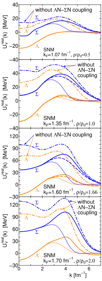
Figure 3: Real part of the $\Lambda$ and $\Sigma$ s.p. potentials in SNM with the chiral NLO YN interactions HAID13 . The solid and dot-dashed curves represent the results of the calculation with switching on and off the $\Lambda$N-$\Sigma$N coupling, respectively. The potentials multiplied by the regularization factor $e^{-(k^{2}/(2\Lambda^{2}))^{3}}$ with $\Lambda=550$ MeV are shown by the dotted curves. The results of the calculation in which the prescription of the regularization is not applied are shown by the dashed curves for $k_{F}=1.35$ and $1.60$ fm^-1.

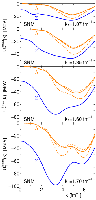
Figure 4: Imaginary part of the $\Lambda$ and $\Sigma$ s.p. potentials in SNM with the chiral NLO YN interactions HAID13 . The short dashed and two-dot-dashed curves stand for the results including the effects from $\Lambda$NN-$\Lambda$NN 3BFs and $\Lambda$NN-$\Sigma$NN 3BFs in addition, respectively, which are discussed in Sec. III.

data MOT88 ; HAS06 , is brought about by the attraction from the coupling. Though the coupling also yields the attraction for the $\Sigma$ hyperon, the $\Sigma$ potential is still positive at the normal density. At low densities, e.g. at $\rho/\rho_{0}=0.5$ in Fig. 3, the $\Sigma$ s.p. potential becomes attractive. These features are also consistent with experimental information SAHA04 ; MK06 .

The partial-wave contributions to the s.p. potential of $\Lambda$ at rest, which are shown in Fig. 5, detail the properties of the NLO $\Lambda$N interaction and the $\Lambda$N-$\Sigma$N coupling. The solid and dashed curves are the results with switching on and off the $\Lambda$N-$\Sigma$N coupling, respectively. The characteristic feature is the density dependence of the ³S₁ contribution when the $\Lambda$N-$\Sigma$N coupling is not taken into account. The repulsion rapidly grows with increasing the density. Although the $\Lambda$N-$\Sigma$N coupling brings about sizable attraction, the attractive $\Lambda$ s.p. potential does not become deeper at greater densities than normal. The attractive contribution in the ¹S₀ state is of the similar order for the ³S₁ contribution, whereas the contributions from other channels are small and do not depend much on the density.

The small splitting of the ³P₁ and ³P₂ contributions in Fig. 5, which is about one third of that for the case of the nucleon, indicates that the $\Lambda$N spin-orbit interaction is not large. However, the experiments have suggested HAS06 that the $\Lambda$N effective spin-orbit interaction is very small. In the analysis of the quark-model $\Lambda$N interaction, it was demonstrated FUJ00 that the antisymmetric spin-orbit component cancels the normal spin-orbit contribution to realize small spin-orbit splitting. In the present NLO $\Lambda$N interaction, there is no antisymmetric spin-orbit component. The possible reduction of the effective $\Lambda$ spin-orbit field by incorporating the contact terms at NLO was discussed by Haidenbauer and Meißner HM15 . It is noted that the 3BFs considered in the next section have normal and antisymmetric spin-orbit components, and they reduce the $\Lambda$N spin-orbit strength by about 10%.

The interesting consequence of these properties of the ChEFT YN interactions is that the depth of the $\Lambda$ s.p. potential does not become deep with increasing the density. This behavior is paved by the density-dependence of the ³S₁ contribution before taking into account the $\Lambda$N-$\Sigma$N coupling. In addition, the $\Lambda$N-$\Sigma$N coupling tends to be suppressed in the nuclear medium with large Fermi momentum by the Pauli blocking for the intermediate nucleon state. The similar behavior is also seen in PNM. The implication of this variation of the $\Lambda$ s.p. potential with respect to the density to the hyperon puzzle is discussed in Sec. IV after including the 3BF effects.

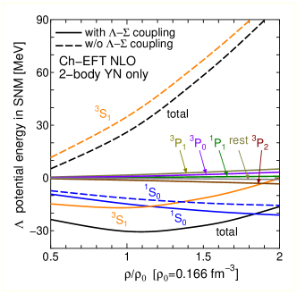
Figure 5: Density-dependence of the partial wave contributions to the $\Lambda$ s.p. potential in SNM with NLO YN interactions HAID13 only.

The imaginary part of the hyperon s.p. potential is related to the spreading width of the hyperon s.p. state in the nuclear medium by $\Gamma=-2\Im U_{Y}$, The vary small width of $\Lambda$ hypernuclear states, in comparison with the nucleon states, has been observed experimentally HAS06 . The reason based on the properties of the YN interaction was discussed in details by Bando et al. BMY85 . Figure 4 shows that the imaginary part of the $\Lambda$ s.p. potential obtained by the ChEFT NLO YN interaction is actually very small, as in other calculations using different YN potentials SCH98 ; KF09 . The strong $\Lambda$N-$\Sigma$N coupling does not directly contribute to the imaginary potential. The imaginary $\Sigma$ potential of $\Im U_{\Sigma}(0)=\sim-15$ to $\sim-20$ MeV is also similar to those with other YN potentials SCH98 ; KF09 .

II.2 Pure neutron matter

In pure neutron matter, the hyperon potential is charge-dependent, and $G$-matrix equations are solved in a particle-base. Because the $\Sigma^{-}$ hyperon does not couple with the $\Lambda$ hyperon, the $\Sigma^{-}$n $G$-matrix is calculated by a single-channel equation. The $\Lambda$ and $\Sigma^{0}$ states are determined through a $\Lambda$n-$\Sigma_{0}$n-$\Sigma^{-}$p coupled equation. The $\Sigma^{+}$ s.p. potential is obtained from a $\Sigma^{+}$n-$\Lambda$p-$\Sigma^{0}$p coupled equation. These $\Lambda$ and $\Sigma^{\pm,0}$ s.p. potentials are determined self-consistently.

The calculated results for $k_{F}^{n}=1.35,1.7$, and 2.0 fm^-1, the neutron densities being $\frac{1}{2}\rho_{0}$, $\rho_{0}$, and $1.63\rho_{0}$, respectively, are shown in Fig. 6. Note that a stable solution was not obtained for the density beyond $k_{F}=2.0$ fm^-1 or $1.6\rho_{0}$. The dashed curves for $\Lambda$, $\Sigma^{0}$, and $\Sigma^{+}$ represent the results in which the $\Lambda$N-$\Sigma$N coupling is switched off. With increasing the density from $k_{F}^{n}=1.35$ to 1.7 fm^-1, the $\Lambda$ s.p. potential at $k=0$ decreases to about $-30$ MeV, and then it turns to become shallower at higher densities, as in SNM.

Because $\Sigma^{-}$ does not couple to $\Lambda$ in PNM, the $\Sigma^{-}$ s.p. potential is resembling to the dot-dashed curve in Fig. 3; that is, repulsive even at low densities. When the $\Sigma$N-$\Lambda$N coupling is ignored, the ordering of the $\Sigma$ s.p. potential is $0<U_{\Sigma^{-}}(0)<U_{\Sigma^{0}}(0)<U_{\Sigma^{+}}(0)$. The $\Sigma^{+}$ s.p. potential is much influenced by the coupling, and the ordering is reversed: $U_{\Sigma^{+}}(0)<0<U_{\Sigma^{0}}(0)<U_{\Sigma^{-}}(0)$. Still, the $\Sigma^{0}$ s.p. potential is considerably repulsive. The increasingly repulsive nature of the $\Sigma^{-}$ and $\Sigma^{0}$ s.p. potentials with growing the density in PNM suggests that the onset of the emergence of these $\Sigma^{-}$ and $\Sigma^{0}$ hyperons in neutron star matter tends to be prevented.

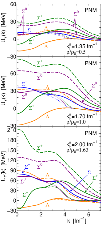
Figure 6: $\Lambda$ and $\Sigma$ s.p. potentials in PNM with the chiral NLO YN interactions HAID13 . Solid curves represent the results including the cutoff form factor for the intermediate potentials in the denominator of the $G$-matrix equation. The latter potentials are shown by the dotted curves. Calculated results with switching off the $\Lambda$N-$\Sigma$N coupling are shown by the dashed curves.

III Including effects of YNN interactions

Leading order three-baryon forces (3BFs) were derived by Petschauer et al. PET16 in SU(3) chiral effective field theory. A feasible way of investigating the effects of these 3BFs to the $\Lambda$ s.p. potential in nuclear matter is to reduce them to density dependent effective two-body interactions by integrating the third nucleon over the occupied states, which may be called as a normal ordered two-body interaction of the original 3BF with respect to nuclear matter. In this article, two-pion exchange $\Lambda$NN-$\Lambda$NN and $\Lambda$NN-$\Sigma$NN 3BFs are taken into consideration, but the $\Sigma$NN-$\Sigma$NN 3BF is left out, because its contribution to the $\Lambda$ s.p. potential is through the correction for the $\Sigma$ s.p. potential in the propagator of the $G$-matrix equation and therefore indirect.

Petschauer et al. PET17 presented the density-dependent effective two-body interactions of the 3BFs in the case of $|\mbox{\boldmath$k$}|=|\mbox{\boldmath$k$}^{\prime}|$ in momentum space, where $k$ and $\mbox{\boldmath$k$}^{\prime}$ are initial and final relative momenta of the two interacting baryons. Here, the expressions for the general case of $|\mbox{\boldmath$k$}|\neq|\mbox{\boldmath$k$}^{\prime}|$ are derived, as in the case of three-nucleon forces MK13 .

III.1 Density-dependent $\Lambda$N-$\Lambda$N interaction from NNLO 2$\pi$-exchange $\Lambda$NN-$\Lambda$NN interaction

Figure 7: $\Lambda$NN-$\Lambda$NN diagrams. The dotted line represents pion exchange. (a) $\Lambda$NN-$\Lambda$NN three-body interaction $V_{TPE}^{\Lambda NN}$, (b) direct term in one-nucleon folding of $V_{TPE}^{\Lambda NN}$, and (c) exchange term in one-nucleon folding of $V_{TPE}^{\Lambda NN}$. $\mbox{\boldmath$k$}_{h}$ indicates an occupied state.

Because there is no $\Lambda\Lambda\pi$ coupling, the two-pion exchange $\Lambda$NN-$\Lambda$NN interaction $V_{TPE}^{\Lambda NN}$ is given by the diagram of Fig. 7(a) alone. Following the expression by Petschauer et al. PET16 , the Born amplitude of this diagram is written as

$$V_{TPE}^{\Lambda NN} =\frac{g_{A}^{2}}{3f_{0}^{4}}\frac{(\mbox{\boldmath$\sigma$}_{3}\cdot\mbox{\boldmath$q$}_{3})(\mbox{\boldmath$\sigma$}_{2}\cdot\mbox{\boldmath$q$}_{2})}{(\mbox{\boldmath$q$}_{3}^{2}+m_{\pi}^{2})(\mbox{\boldmath$q$}_{2}^{2}+m_{\pi}^{2})}(\mbox{\boldmath$\tau$}_{2}\cdot\mbox{\boldmath$\tau$}_{3})$$

$$\times\{-(3b_{0}+b_{D})m_{\pi}^{2}+(2b_{2}+3b_{4})\mbox{\boldmath$q$}_{3}\cdot\mbox{\boldmath$q$}_{2}\},$$ (1)

where the coordinate 1 is assigned to the $\Lambda$ hyperon and $\mbox{\boldmath$q$}_{2}$ ($\mbox{\boldmath$q$}_{3}$) is the difference of the final and initial momenta at the nucleon line 2 (line 3). $g_{A}$ is the axial coupling constant, $f_{0}$ is the pion decay constant, $m_{\pi}$ is the pion mass, and $\sigma$ and $\tau$ stand for the spin and isospin operators. The coupling constants $b_{0}$, $b_{D}$, $b_{2}$, and $b_{4}$ inherit those in the underlying Lagrangian. This 3BF is reduced to an effective $\Lambda$N-$\Lambda$N interaction $V_{TPE}^{\Lambda N(N)}$ by folding one nucleon degrees of freedom over the occupied states in nuclear matter. Assuming that two baryons are in the center of mass frame, the effective two-body matrix element from $V_{TPE}^{\Lambda NN}$ is obtained as

$$\langle\mbox{\boldmath$k$}^{\prime}\sigma_{\Lambda}^{\prime},-\mbox{\boldmath$k$}^{\prime}\sigma^{\prime}\tau^{\prime}|V_{\Lambda N(N)}|\mbox{\boldmath$k$}\sigma_{\Lambda},-\mbox{\boldmath$k$}\sigma\tau\rangle$$

$$=\frac{g_{A}^{2}}{3f_{0}^{4}}\sum_{\mbox{\boldmath$k$}_{h}}\sum_{\sigma_{h},\tau_{h}}\langle\mbox{\boldmath$k$}^{\prime}\sigma_{\Lambda},-\mbox{\boldmath$k$}^{\prime}\sigma^{\prime}\tau^{\prime},\mbox{\boldmath$k$}_{h}\sigma_{h}\tau_{h}|(\mbox{\boldmath$\tau$}_{2}\cdot\mbox{\boldmath$\tau$}_{3})$$

$$\times\frac{(\mbox{\boldmath$\sigma$}_{3}\cdot(-\mbox{\boldmath$k$}^{\prime}-\mbox{\boldmath$k$}_{h}))(\mbox{\boldmath$\sigma$}_{2}\cdot(\mbox{\boldmath$k$}_{h}+\mbox{\boldmath$k$}))}{((\mbox{\boldmath$k$}_{h}+\mbox{\boldmath$k$}^{\prime})^{2}+m_{\pi}^{2})((\mbox{\boldmath$k$}_{h}+\mbox{\boldmath$k$})^{2}+m_{\pi}^{2})}$$

$$\times\{-(3b_{0}+b_{D})m_{\pi}^{2}+(2b_{2}+3b_{4})(-\mbox{\boldmath$k$}_{h}-\mbox{\boldmath$k$}^{\prime})\cdot(\mbox{\boldmath$k$}_{h}+\mbox{\boldmath$k$})\}$$

$$\times|(\mbox{\boldmath$k$}\sigma_{\Lambda},-\mbox{\boldmath$k$}\sigma\tau,\mbox{\boldmath$k$}_{h}\sigma_{h}\tau_{h})-(\mbox{\boldmath$k$}\sigma_{\Lambda},\mbox{\boldmath$k$}_{h}\sigma_{h}\tau_{h},-\mbox{\boldmath$k$}\sigma\tau)\rangle,$$ (2)

where $\mbox{\boldmath$k$}_{h}$, $\sigma_{h}$ and $\tau_{h}$ specify the nucleon in momentum, spin, and isospin states. In the following, $\tau=-1/2$ is assigned for neutron and $\tau=1/2$ proton. The diagrammatic representation of the integration is depicted in Figs. 7(b) and 7(c). The direct term, Fig. 7(b), vanishes because of the spin summation. The isospin summation in the exchange contribution gives $\sum_{\tau_{h}}\langle\tau^{\prime}\tau_{h}|(\mbox{\boldmath$\tau$}_{2}\cdot\mbox{\boldmath$\tau$}_{3})|\tau_{h}\tau\rangle=3\delta_{\tau^{\prime}\tau}$ in SNM, and $\{1\delta_{\tau^{\prime}-1/2}\delta_{\tau,-1/2}+2\delta_{\tau^{\prime},1/2}\delta_{\tau,1/2}\}$ in PNM. While central, spin-orbit, and antisymmetric spin-orbit components appear from $V_{TPE}^{\Lambda NN}$, no tensor component is generated. Explicit expressions after carrying out the spin-summation and $\mbox{\boldmath$k$}_{h}$ integration are given in Appendix. If the condition of $|\mbox{\boldmath$k$}^{\prime}|=|\mbox{\boldmath$k$}|$ is imposed for the expression in Appendix, the results agree with those given by Petschauer et al. PET17 . It should be noted that a statistical factor of $\frac{1}{2}$ has to be multiplied when the effective two-body interaction defined by Eq. 2 is added to the original two-body $\Lambda$N-$\Lambda$N interaction. It is worthwhile to mention that in the case of three-nucleon forces the statistical factor is $\frac{1}{3}$ for the total energy in the Hartree-Fock level and $\frac{1}{2}$ for the s.p. energy, whereas here the factor of $\frac{1}{2}$ is common for the total and s.p. energies.

As for a form factor, it is not included in the stage of the integration of Eq. 2, but the resulting effective two-body interaction $V_{\Lambda N(N)}$ is multiplied by the following Gaussian regularization factor same as in the NN sector with the cutoff scale $\Lambda$ being 550 MeV:

$$\exp(-(k^{\prime}/\Lambda)^{6}-(k/\Lambda)^{6}).$$ (3)

The normal-ordered interaction $V_{\Lambda N(N)}$ can be regarded as a Pauli-blocking effect for the two-pion exchange two-body $\Lambda$N interaction with the $\pi\pi\Lambda\Lambda$ vertex. Supposing that this two-pion exchange $\Lambda$N interaction provides an attractive component, the Pauli-blocking brings about repulsion.

III.2 Density-dependent $\Lambda$N-$\Sigma$N interaction from NLO $\Lambda$NN-$\Sigma$NN interaction

Figure 8: $\Lambda$NN-$\Sigma$NN diagrams. The dotted line represents pion exchange. (a) 3BF $V_{TPE,a}^{\Lambda-\Sigma}$ with $\pi\pi\Lambda\Sigma$ vertex, (b) 3BF $V_{TPE,b}^{\Lambda-\Sigma}$ with $\pi\Lambda\Sigma$ vertex, (c) direct term in one-nucleon folding of $V_{TPE,a}^{\Lambda-\Sigma}$, and (d) exchange term in one-nucleon folding of $V_{TPE,a}^{\Lambda-\Sigma}$, (e) direct term in one-nucleon folding of $V_{TPE,b}^{\Lambda-\Sigma}$, (f) exchange term in one-nucleon folding of $V_{TPE,b}^{\Lambda-\Sigma}$, and (g) exchange term in one-nucleon folding of $V_{TPE,a}^{\Lambda-\Sigma}$. $\mbox{\boldmath$k$}_{h}$ indicates an occupied state.

As for the $\Lambda$NN-$\Sigma$NN transition process, in addition to the diagram Fig. 8(a), there appears another type of the diagram presented in Fig. 8(b) . Besides, the amplitude of the diagram of Fig. 8(a) has an extra term;

$$V_{TPE,a}^{\Lambda-\Sigma} =-\frac{1}{4f_{0}^{4}}\frac{(\mbox{\boldmath$\sigma$}_{2}\cdot\mbox{\boldmath$q$}_{2})(\mbox{\boldmath$\sigma$}_{3}\cdot\mbox{\boldmath$q$}_{3})}{(\mbox{\boldmath$q$}_{2}^{2}+m_{\pi}^{2})(\mbox{\boldmath$q$}_{3}^{2}+m_{\pi}^{2})}i(\mbox{\boldmath$\Sigma$}\cdot(\mbox{\boldmath$\tau$}_{2}\times\mbox{\boldmath$\tau$}_{3}))$$

$$\times[N_{1}^{a}+N_{2}^{a}(\mbox{\boldmath$q$}_{2}\cdot\mbox{\boldmath$q$}_{3})+N_{3}^{a}i(\mbox{\boldmath$\sigma$}_{1}\cdot(\mbox{\boldmath$q$}_{2}\times\mbox{\boldmath$q$}_{3})].$$ (4)

The amplitude of the diagram of Fig. 8(b) has the following structure;

$$V_{TPE,b}^{\Lambda-\Sigma} =-\frac{1}{4f_{0}^{4}}\frac{(\mbox{\boldmath$\sigma$}_{1}\cdot\mbox{\boldmath$q$}_{1})(\mbox{\boldmath$\sigma$}_{3}\cdot\mbox{\boldmath$q$}_{3})}{(\mbox{\boldmath$q$}_{1}^{2}+m_{\pi}^{2})(\mbox{\boldmath$q$}_{3}^{2}+m_{\pi}^{2})}$$

$$\times[(\mbox{\boldmath$\Sigma$}\cdot\mbox{\boldmath$\tau$}_{3})\{N_{1}^{b}+N_{2}^{b}(\mbox{\boldmath$q$}_{1}\cdot\mbox{\boldmath$q$}_{3})\}$$

$$-N_{3}^{b}((\mbox{\boldmath$\Sigma$}\times\mbox{\boldmath$\tau$}_{3})\cdot\mbox{\boldmath$\tau$}_{2})((\mbox{\boldmath$q$}_{1}\times\mbox{\boldmath$q$}_{3})\cdot\mbox{\boldmath$q$}_{2})].$$ (5)

In the above expressions, $\Sigma$ represents the isospin operator asociated with the $\Lambda$-$\Sigma$ transition, and the explicit values of the coupling constants $N_{1\sim 3}^{a}$ and $N_{1\sim 3}^{b}$ are given in the next subsection.

To obtain effective two-body interactions from these 3BFs, the following matrix element is calculated in which both the bra and ket states are anti-symmetrized with respect to the two nucleons.

$$\langle\mbox{\boldmath$k$}^{\prime}\sigma_{\Sigma}\tau_{\Sigma},-\mbox{\boldmath$k$}^{\prime}\sigma^{\prime}\tau^{\prime}|V_{\Lambda N(N)-\Sigma N(N)}|\mbox{\boldmath$k$}\sigma_{\Lambda},-\mbox{\boldmath$k$}\sigma\tau\rangle$$

$$\sum_{\mbox{\boldmath$k$}_{h}}\sum_{\sigma_{h},\tau_{h}}\left(\frac{1}{\sqrt{2}}\right)^{2}\langle(\mbox{\boldmath$k$}^{\prime}\sigma_{\Sigma}\tau_{\Sigma},-\mbox{\boldmath$k$}^{\prime}\sigma^{\prime}\tau^{\prime},\mbox{\boldmath$k$}_{h}\sigma_{h}\tau_{h})$$

$$-(\mbox{\boldmath$k$}^{\prime}\sigma_{\Sigma}\tau_{\Sigma},\mbox{\boldmath$k$}_{h}\sigma_{h}\tau_{h},-\mbox{\boldmath$k$}^{\prime}\sigma^{\prime}\tau^{\prime})|V_{TPE}^{\Lambda-\Sigma}$$

$$\times|(\mbox{\boldmath$k$}\sigma_{\Lambda},-\mbox{\boldmath$k$}\sigma\tau,\mbox{\boldmath$k$}_{h}\sigma_{h}\tau_{h})-(\mbox{\boldmath$k$}\sigma_{\Lambda},\mbox{\boldmath$k$}_{h}\sigma_{h}\tau_{h},-\mbox{\boldmath$k$}\sigma\tau)\rangle.$$ (6)

Explicit expressions after carrying out the spin-summation and $\mbox{\boldmath$k$}_{h}$ integration are given in Appendix. When the condition of $|\mbox{\boldmath$k$}^{\prime}|=|\mbox{\boldmath$k$}|$ is imposed for the expression in Appendix, the expression given by Petschauer et al. PET17 is reproduced. Again, an additional statistical factor of $\frac{1}{2}$ is multiplied, when it is incorporated to the original two-body $\Lambda$N-$\Sigma$N transition interaction.

III.3 Assignment of low-energy-constants in 3B YNN interactions

The low energy constants in Eq. (1) were estimated in Ref. PET17 by adopting decouplet saturation. Numerical values are

$$-(3b_{0}+b_{D})=0,\hskip 10.00002pt2b_{2}+3b_{4}=-\frac{C^{2}}{\Delta}\approx-3.0\;\mbox{GeV}^{-1},$$ (7)

where $C=\frac{3}{4}g_{A}$ and $\Delta$ is the average decouplet-octet mass splitting of about 300 MeV. The coupling constants contained in Eq. (4) are estimated as

$$N_{1}^{a}=N_{2}^{a}=0,\hskip 10.00002ptN_{3}^{a}=-\frac{4g_{A}^{2}}{3}\frac{C^{2}}{\Delta}\approx-6.7\;\mbox{GeV}^{-1}.$$ (8)

Similarly, those in Eq. (5) are

$$N_{1}^{b} =0,\hskip 10.00002ptN_{2}^{b}=-4\frac{8Dg_{A}}{9}\frac{C^{2}}{\Delta}\approx-10.7\;\mbox{GeV}^{-1},$$

$$N_{3}^{b} =-4\frac{8Dg_{A}}{9}\frac{C^{2}}{\Delta}\approx-2.7\;\mbox{GeV}^{-1},$$ (9)

where $D$ is an SU(3) $D$-type coupling constant and has a relation $D+F=g_{A}$ with the $F$-type coupling constant.

The nucleon part of the diagram of Fig. 8(b) is the same as that in the nucleon two-pion exchange 3NF. Namely, the diagram of Fig. 8(b) is obtained by replacing the $\pi NN$ vertex in 3BFs by the $\pi\Lambda\Sigma$ vertex. Therefore, the corresponding coupling constants used in the nucleon sector may be employed. Then the following estimation is possible:

$$N_{1}^{b} =-Dg_{A}4c_{1}m_{\pi}^{2}=1.6\;\mbox{GeV}^{-1},$$

$$N_{2}^{b} =2Dg_{A}c_{3}=-6.8\;\mbox{GeV}^{-1}$$

$$N_{3}^{b} =-Dg_{A}c_{4}=-3.4\;\mbox{GeV}^{-1}.$$ (10)

It is reassuring to find that the corresponding numbers of Eqs. (8) and (10) are of the same order. In the numerical evaluations in the next section, the values in Eqs. (7), (8), and (9) are used.

The diagram of Fig. 8(d) is a medium modification of the two-pion exchange $\Lambda$N-$\Sigma$N transition by Pauli blocking. This effect is expected to enhance the tensor component. Figure 8(f) is a modification of the pion propagation and Figs. 8(g) and 8(h) are regarded as a correction for the $\pi NN$ vertex in the nuclear medium.

IV Numerical results of YNN contributions

Including the normal-ordered two-body interactions of the 3BFs, s.p. potentials of the $\Lambda$ and $\Sigma$ hyperons are evaluated in SNM and PNM. Contributions of the $\Lambda$NN-$\Lambda$NN 3BFs are first presented, and then the effects of the $\Lambda$NN-$\Sigma$NN transition interactions are incorporated.

IV.1 2$\pi$-exchange $\Lambda$NN-$\Lambda$NN interaction

It is instructive to estimate the effect of the $\Lambda$NN-$\Lambda$NN 3BFs to the $\Lambda$ s.p. potential by considering their contribution on the Hartree-Fock level. Namely, the following summation over two nucleons in occupied states is evaluated.

$$\Delta U_{\Lambda}(k_{\Lambda})=\frac{1}{2}\sum_{\sigma_{\Lambda}}\frac{1}{2}\sum_{|\mbox{\boldmath$k$}|\leq k_{F},\sigma,\tau}\sum_{|\mbox{\boldmath$k$}^{\prime}|\leq k_{F},\sigma^{\prime},\tau^{\prime}}$$

$$\times\langle\mbox{\boldmath$k$}_{\Lambda}\sigma_{\Lambda},\mbox{\boldmath$k$}\sigma\tau,\mbox{\boldmath$k$}^{\prime}\sigma^{\prime}\tau^{\prime}|V_{TPE}^{\Lambda NN}$$

$$\times|(\mbox{\boldmath$k$}_{\Lambda}\sigma_{\Lambda},\mbox{\boldmath$k$}\sigma\tau,\mbox{\boldmath$k$}^{\prime}\sigma^{\prime}\tau^{\prime})-(\mbox{\boldmath$k$}_{\Lambda}\sigma_{\Lambda},\mbox{\boldmath$k$}^{\prime}\sigma^{\prime}\tau^{\prime},\mbox{\boldmath$k$}\sigma\tau)\rangle.$$ (11)

When the cutoff form factor is disregarded, the result does not depend on $k_{\Lambda}$ and the summation can be carried out analytically to yield

$$\Delta U_{\Lambda}=-\frac{g_{A}^{2}}{3f_{0}^{4}}\frac{1}{(2\pi)^{6}}F_{\tau}\frac{4\pi^{2}}{3}\left[\rule[0.0pt]{0.0pt}{15.00002pt}(3b_{0}+b_{D})m_{\pi}^{2}\right.$$

$$\times\left\{\frac{3}{2}k_{F}^{2}(2k_{F}^{2}-m_{\pi}^{2})+\frac{3}{8}m_{\pi}^{2}(8k_{F}^{2}+m_{\pi}^{2})\log\frac{4k_{F}^{2}+m_{\pi}^{2}}{m_{\pi}^{2}}\right.$$

$$\left.-6m_{\pi}k_{F}^{3}\arctan\frac{2k_{F}}{m_{\pi}}\right\}$$

$$+(2b_{2}+3b_{4})\left\{-\frac{1}{2}m_{\pi}^{4}(9k_{F}^{2}+m_{\pi}^{2})\log\frac{4k_{F}^{2}+m_{\pi}^{2}}{m_{\pi}^{2}}\right.$$

$$\left.\left.+\frac{2}{3}k_{F}^{2}(2k_{F}^{4}-9m_{\pi}^{2}k_{F}^{2}+3m_{\pi}^{4})+10m_{\pi}^{3}k_{F}^{3}\arctan\frac{2k_{F}}{m_{\pi}}\right\}\right].$$ (12)

where $F_{\tau}$ is a factor from isospin summation: $F_{\tau}=6$ in SNM and $F_{\tau}=1$ in PNM.

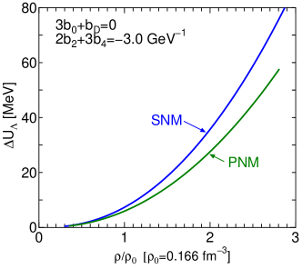
Figure 9: $k_{F}$ dependence of $\Delta U_{\Lambda}$, Eq. 12, in SNM and in PNM. Coupling constants estimated by Petschauer et al. PET17 are employed.

The $k_{F}$ dependence of $\Delta U_{\Lambda}$ is shown in Fig. 9 both for SNM and PNM. Using the low-energy constants of Eq. (7), the repulsive effect from the $\Lambda$NN-$\Lambda$NN interaction is about 7 MeV at the normal density in SNM and grows rapidly with increasing the density. It can be numerically proved that the inclusion of a cutoff form factor of the form of $\exp[-\frac{1}{36\Lambda_{3BF}^{4}}\{(\mbox{\boldmath$k$}_{\Lambda}-\mbox{\boldmath$k$})^{2}+(\mbox{\boldmath$k$}_{\Lambda}-\mbox{\boldmath$k$}^{\prime})^{2}+(\mbox{\boldmath$k$}-\mbox{\boldmath$k$}^{\prime})^{2}\}^{2}]$ modifies the result little, with the cutoff momentum of $\Lambda_{3BF}\approx 500$ MeV.

The $\Lambda$N ladder correlation by the $G$-matrix equation is expected to somewhat reduce the repulsive effect of the $\Lambda$NN-$\Lambda$NN interaction. Although the 3BF in ChEFT is not applicable beyond the cutoff momentum scale, the considerably repulsive effect without an ad hoc phenomenological parameterization is suggestive for the properties of the $\Lambda$ hyperon in high density nuclear matter, together with the shallow $\Lambda$ s.p. potential presented in the previous section.

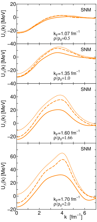
Figure 10: Real part of the $\Lambda$ s.p. potentials in SNM with the chiral NLO YN interactions HAID13 . The solid curves are the same as in Fig. 3; that is, without the effects of 3BFs. The dotted curves stand for the results including the effects of $\Lambda$NN-$\Lambda$NN 3BFs. The dashed curves represent the results, including the both effects of $\Lambda$NN-$\Lambda$NN and $\Lambda$NN-$\Sigma$NN 3BFs.

Now, the results of the $\Lambda$ s.p, potential obtained from the actual $G$-matrix calculations, in which the effective two-body interaction $V_{\Lambda N(N)}$ is incorporated, are shown by the dotted curves in Fig. 10 for SNM and in Fig. 11 for PNM. As noted earlier, stable results are not available at high densities. The upper limit of the Fermi momentum is $k_{F}=1.70$ fm^-1 in SNM and $k_{F}^{n}=2.00$ fm^-1 in PNM. The $\Sigma$ s.p. potential is not shown, because the $\Sigma$NN-$\Sigma$NN 3BFs are not considered and the change due to the variation of the $\Lambda$ s.p. potential is very small. The repulsive effect of the $\Lambda$NN-$\Lambda$NN interaction is about 5 MeV at the normal density and about 20 MeV at $2\rho_{0}$ in SNM. The similar repulsive contribution is also obtained in PNM. Compared with $\Delta U_{\Lambda}$ in Fig. 9, the $G$-matrix ladder correlation reduces the repulsion by $30\sim 40$ %.

In this article, the one-pion exchange contact and three-body contact terms of the leading order YNN interactions are not considered. The estimation of their role by Haidenbauer et al. Ref. HMKW17 shows that the attractive contribution can be obtained to compensate the repulsive $\Lambda$NN-$\Lambda$NN effect by tuning the sign of the coupling constants. Before quantifying these contributions, however, it is better to investigate the effect of the $\Lambda$NN-$\Sigma$NN 3BFs.

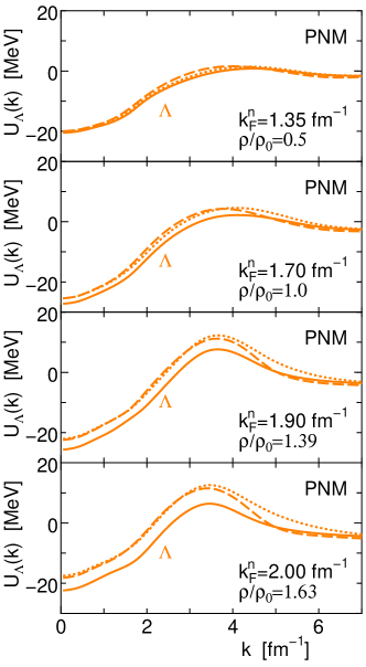
Figure 11: Same as Fig. 10 but for PNM.

IV.2 2$\pi$-exchange $\Lambda$NN-$\Sigma$NN interaction

Results of the $G$-matrix calculations including the effects both from the $\Lambda$NN-$\Sigma$NN and $\Lambda$NN-$\Sigma$NN 3BFs are presented by the dashed curves in Fig. 10 for SNM and in Fig. 11 for PNM.

It is interesting to observe that the net attractive contribution from the $\Lambda$NN-$\Sigma$NN coupling almost cancels the repulsive effect of the $\Lambda$NN-$\Lambda$NN 3BFs at the normal density in SNM, and the potential depth of the $\Lambda$ hyperon remains to be consistent with experimental data. At higher densities, however, the cancellation is incomplete and the net 3BF contribution is repulsive. In PNM, on the other hand, the effect of the $\Lambda$NN-$\Sigma$NN 3BFs is very small, and therefore does not weaken the repulsion from the $\Lambda$NN-$\Lambda$NN 3BFs.

IV.3 Relevance to the role of $\Lambda$ in neutron star matter

The $\Lambda$ s.p. potential in the nuclear medium is closely related to the possible role of the $\Lambda$ hyperons in neutron star matter. Although the mixture of protons has to be taken into account in the realistic study of neutron star matter, it is helpful to examine the density-dependence of the neutron chemical potential $\mu_{n}$ and the $\Lambda$ s.p. potential $U_{\Lambda}(0)$ at rest in PNM. Considering the $\Lambda$-neutron mass difference $\Delta m=m_{\Lambda}-m_{n}=176.1$ MeV, the simple condition for the emergence of the $\Lambda$ hyperon in PNM is

$$U_{\Lambda}(0)<\mu_{n}-\Delta m$$ (13)

Although the present calculations with the interactions in ChEFT are limited to the densities below $1.63\rho_{0}$, it is worth considering the implication of the density-dependence of the present $U_{\Lambda}(0)$. Figure 12 shows the density-dependence of the calculated $U_{\Lambda}(0)$ and that of $\mu_{n}-m_{\Delta}=\frac{\hbar^{2}}{2m_{n}}(k_{F}^{n})^{2}+U_{n}(k_{F}^{n})-\Delta m$. The solid and dashed curves of $U_{\Lambda}(0)$ are the results with and without including YNN 3BF effects, respectively. To see the difference of the ChEFT YN interaction from other YN potentials, two curves are included, showing the results of the Brueckner-Hartree-Fock (BHF) calculations by Schulze and Rijken SCH11 with employing the Nijmegen YN potentials NSC89 NIJ89 and ESC08 RNY10 , in which YNN 3BFs are not taken into account.

For the neutron chemical potential $\mu_{n}$, three cases of the ChEFT cutoff scale, $\Lambda=450$, 550, and 600 MeV, are presented up to the density $1.63\rho_{0}$, $1.63\rho_{0}$, and $1.19\rho_{0}$, respectively. For comparison, typical other nucleon chemical potentials are included in Fig. 12, which are evaluated by $\mu_{\Lambda}=\frac{\partial\epsilon(\rho_{n},\rho_{\Lambda})}{\partial\rho_{\Lambda}}$ at $\rho_{\Lambda}=0$, using the energy density $\epsilon(\rho_{n},\rho_{\Lambda})$ found in the literature. The dashed curve denotes $\mu_{n}$ evaluated from the parameterization of the energy density of the model A18+$\delta v$+UIX* given in Appendix of the article by Akmal, Pandharipande, and Ravenhall APR98 on the basis of .the variational calculation with AV18 AV18 NN force + Urbana model IX 3BF PPCW95 . The short dashed curve is obtained by the parameterization by Schulze and Rijken SCH11 , which is based on the BHF calculation with AV18 AV18 + UIX’ 3BF ZH04 . The EOS corresponding to these $\mu_{n}$ may not be stiff enough to support a neutron star with a mass of 2$M_{\odot}$ SCH11 , but serves as a standard EOS with which various models of the neutron matter EOS in the literature can be compared.

The curves of $U_{\Lambda}(0)$ with NSC98 and ESC08 cross the curve of the standard $\mu_{n}$ below the neutron matter density of $2.5\rho_{0}$. The onset of the $\Lambda$ emergence makes the EOS appreciably soft, with which a heavy neutron star with a mass of $2M_{\odot}$ cannot be held. It is a natural hypothesis to include strongly repulsive $\Lambda$NN 3BF LON15 ; YAM14 to avoid the $\Lambda$ emergence or to make the EOS stiff enough even under the presence of $\Lambda$ hyperons. The present chiral YN interactions suggest a somewhat different possibility. The dashed curve in Fig. 12 indicates that the $\Lambda$ s.p. potential is considerably shallow. The naive extrapolation of the dashed curve to the higher density region may not cross the curve of the standard $\mu_{n}$. The 3BFs constructed systematically in ChEFT provides an additional repulsive effect, which can be sizable at higher densities as Fig. 9 denotes. Supposing that it may not be appropriate to discuss neutron star matter at densities beyond $3\sim 4\rho_{0}$ by a solely hadronic picture, the non-emergence of the $\Lambda$ hyperon below the density of $3\sim 4\rho_{0}$ can be a solution of the hyperon puzzle.

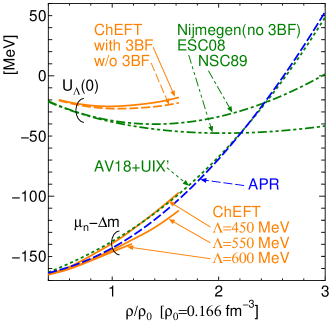
Figure 12: $k_{F}$ dependence of $U_{\Lambda}(0)$ and $\mu_{n}-\Delta m$ in PNM. Solid and dashed curves for the $U_{\Lambda}(0)$ stand for the results with and without 3BF contribution, respectively. The dashed curve is based on the energy density parameterized by Akmal, Pandharipande, and Ravenhall APR98 , and the short dashed curve is evaluated by the parameterization by Schulze and Rijken SCH11 . The dot-dashed curve and the two-dot-dashed curve for $U_{\Lambda}(0)$ are calculated using the energy densities by Schulze and Rijken SCH11 .

V Summary

Single-particle potentials of the $\Lambda$ and $\Sigma$ hyperons in SNM and in PNM are calculated in the standard LOBT framework, using YN interactions HAID13 constructed in chiral effective field theory at the NLO level. Contributions of the NNLO YNN 3BFs PET16 are also considered in the normal-ordering prescription. In addition to the effects of the $\Lambda$NN-$\Lambda$NN 3BF, those of the $\Lambda$NN-$\Sigma$NN transition 3BF are incorporated. The $\Lambda$N-$\Sigma$N coupling is known to be important because of the tensor component from the pion exchange. Compared with other YN potentials, the ChEFT YN interaction bears particularly strong $\Lambda$N-$\Sigma$N coupling. The $\Lambda$ s.p. potential is repulsive when the $\Lambda$N-$\Sigma$N coupling is switched off. The $\Lambda$ s.p. potential of about $-30$ MeV at the normal density, which is consistent with the empirical data, originates from the $\Lambda$N-$\Sigma$N coupling. The $\Sigma$ potential is weakly attractive at the low densities in SNM, but becomes repulsive with increasing the density. This feature is consistent with the empirical data. The $\Sigma$ potential hight in SNM and the $\Sigma^{-}$ potential hight in PNM grow rapidly as the density increases.

The salient feature of the NLO YN interaction is that the $\Lambda$ s.p. potential becomes shallower at greater than normal density. This behavior is paved by the density dependence of the contribution of the $\Lambda$N-$\Lambda$N interaction in the ³S₁ channel. In addition, the $\Lambda$N-$\Sigma$N coupling bringing about the substantial attraction tends to be suppressed by Pauli blocking when the Fermi momentum becomes larger. The situation is same in PNM, which is more relevant to neutron star matter.

It has been expected that the $\Lambda$ hyperons appear in high-density neutron star matter to bypass the neutron chemical potential, and therefore the equation of state of PNM becomes soft. The recent observation of twice the solar-mass neutron stars has imposed a constraint for the stiffness of the EOS, with which naive emergence of hyperons seems to be excluded. This contradictory situation is called hyperon puzzle. The character of the $\Lambda$ s.p. potential predicted by the NLO ChEFT suggests that the $\Lambda$ hyperon is energetically not favored in neutron star matter at higher densities. Because ChEFT is effective low-energy theory, the cutoff scale being of the order of 500 MeV, it is not adequate to discuss the region of the density greater than $2\sim 2.5$ times normal density. Nevertheless, the behavior of the $\Lambda$ s.p. potential below the limit is suggestive, and the ChEFT YN interaction provides a possibility to resolve the hyperon puzzle.

The effects of the two-pion exchange $\Lambda$NN-$\Lambda$NN 3B interactions make the $\Lambda$ s.p. potential less attractive. To be consistent with the empirical data, the attraction which compensates this repulsive contribution is required. It is conceivable to include the $\Lambda$NN-$\Lambda$NN contact terms, as was practiced by Haidenbauer et al. HMKW17 , and tune the coupling constants. In this article, before introducing those contact terms, contributions from the $\Lambda$NN-$\Sigma$NN transition 3BF are investigated. It is demonstrated that the effects of the effective $\Lambda$N-$\Sigma$N interactions from the $\Lambda$NN-$\Sigma$NN processes serve to restore the $\Lambda$ potential depth of about 30 MeV at the normal density in SNM. At the densities greater than the normal, the net contribution from the YNN interaction is repulsive of the order of $5\sim 10$ MeV, which supports to disfavor the emergence of the $\Lambda$ hyperon in high-density neutron star matter.

It is known in the non-strange sector that higher orders in ChEFT beyond NLO are important. In the future, the inclusion of higher order terms is necessary also in the strangeness sector, although at present it is not meaningful because of the insufficiency of experimental data on the amount as well as the accuracy. YNN 3BFs of $K$ and $\eta$ meson exchange processes are better to be considered. In parallel with these developments, it is also important to examine the properties of the ChEFT YN interactions by investigating experimental data of hyper nuclei, which will be provided by the on-going and future experiments.

.1 Effective 2B interaction from the $\Lambda$NN-$\Lambda$NN interaction

The evaluation of Eq. (2) becomes

$$\frac{g_{A}^{2}}{3f_{0}^{4}}C_{\tau}^{\Lambda\Lambda}(3b_{0}+b_{D})m_{\pi}^{2}\sum_{\ell=0}^{\infty}\hat{\ell}P_{\ell}(\cos\theta)\left[\cos\theta\;Q_{W0}^{\ell}(k^{\prime},k)-\{Q_{X1}^{\ell}(k,k^{\prime})+Q_{X1}^{\ell}(k^{\prime},k)-\delta_{\ell 0}\frac{1}{2}(F_{0}(k^{\prime})+F_{0}(k))\}\right]$$

$$-\frac{g_{A}^{2}}{3f_{0}^{4}}3(2b_{2}+3b_{4})\left\{\frac{1}{8}\rho_{0}-\frac{1}{4}(2k^{\prime 2}+k^{2}+3m_{\pi}^{2})F_{0}(k^{\prime})-\frac{1}{4}(k^{\prime 2}+2k^{2}+3m_{\pi}^{2})F_{0}(k)\right.$$

$$+\frac{1}{4}(k^{\prime 2}F_{2}(k^{\prime})+k_{1}^{2}F_{2}(k))+k^{\prime}kP_{1}(\cos\theta)\left[F_{0}(k^{\prime})+F_{0}(k)-\frac{1}{2}(F_{1}(k^{\prime})+F_{1}(k)))\right]$$

$$\left.+\frac{1}{4}\left(2m_{\pi}^{2}+k^{\prime 2}+k^{2}-2k^{\prime}k\cos\theta\right)^{2}\frac{1}{k^{\prime}k}\sum_{\ell}\hat{\ell}P_{\ell}(\cos\theta)Q_{W0}^{\ell}(k^{\prime},k)\right\}$$

$$+\frac{g_{A}^{2}}{3f_{0}^{4}}3(i\mbox{\boldmath$\sigma$}_{N}\cdot(\mbox{\boldmath$k$}^{\prime}\times\mbox{\boldmath$k$}))(3b_{0}+b_{D})m_{\pi}^{2}\frac{1}{k^{\prime}k}\sum_{\ell=0}^{\infty}\left\{\hat{\ell}P_{\ell}(\cos\theta)Q_{W0}^{\ell}(k^{\prime},k)\right.$$

$$\left.+P_{\ell}^{\prime}(\cos\theta)(Q_{W1}^{\ell,\ell+1}(k,k^{\prime})+Q_{W1}^{\ell,\ell+1}(k^{\prime},k)-Q_{W1}^{\ell,\ell-1}(k,k^{\prime})-Q_{W1}^{\ell,\ell-1}(k^{\prime},k))\right\}$$

$$-\frac{g_{A}^{2}}{3f_{0}^{4}}3(2b_{2}+3b_{4})(i\mbox{\boldmath$\sigma$}_{N}\cdot(\mbox{\boldmath$k$}^{\prime}\times\mbox{\boldmath$k$}))\left[\frac{1}{2}(F_{0}(k^{\prime})+F_{0}(k)-F_{1}(k^{\prime})-F_{1}(k))-\frac{((\mbox{\boldmath$k$}^{\prime}-\mbox{\boldmath$k$})^{2}+2m_{\pi}^{2})}{2k^{\prime}k}\sum_{\ell=0}^{\infty}\right.$$

$$\left.\times\{\hat{\ell}P_{\ell}(\cos\theta)Q_{W0}^{\ell}(k^{\prime},k)+P_{\ell}^{\prime}(\cos\theta)(Q_{W1}^{\ell,\ell+1}(k,k^{\prime})+Q_{W1}^{\ell,\ell+1}(k^{\prime},k)-Q_{W1}^{\ell,\ell-1}(k,k^{\prime})-Q_{W1}^{\ell,\ell-1}(k^{\prime},k))\}\right],$$ (14)

where $P_{\ell}(\cos\theta)$ is a Legendre function and $\theta$ is the angle between $\mbox{\boldmath$k$}^{\prime}$ and $k$. Definitions of $F_{0}$, $F_{1}$, $F_{2}$, $Q_{W0}^{\ell}$, $Q_{W1}^{\ell}$, and $Q_{W1}^{\ell,\ell+1}$ are given in Ref. [24]. The constant $C_{\tau}^{\Lambda\Lambda}$ comes from the isospin summation: $C_{\tau}^{\Lambda\Lambda}=3\delta_{\tau^{\prime}\tau}$ in SNM and $C_{\tau}^{\Lambda\Lambda}=\{1\delta_{\tau^{\prime}-1/2}\delta_{\tau-1/2}+2\delta_{\tau 1/2}\delta_{\tau 1/2}\}$ in PNM. If the condition $|\mbox{\boldmath$k$}|=|\mbox{\boldmath$k$}^{\prime}|$ is applied for the initial and final momenta, $k$ and $\mbox{\boldmath$k$}^{\prime}$, the expression given by Petschauer et al. [31] is recovered. The term including $(i\mbox{\boldmath$\sigma$}_{2}\cdot(\mbox{\boldmath$k$}^{\prime}\times\mbox{\boldmath$k$}))$ gives normal and anti-symmetric spin-orbit components:

$$i\mbox{\boldmath$\sigma$}_{N}\cdot(\mbox{\boldmath$k$}^{\prime}\times\mbox{\boldmath$k$})=-i\frac{1}{2}(\mbox{\boldmath$\sigma$}_{\Lambda}+\mbox{\boldmath$\sigma$}_{N})\cdot(\mbox{\boldmath$k$}\times\mbox{\boldmath$k$}^{\prime})+i\frac{1}{2}(\mbox{\boldmath$\sigma$}_{\Lambda}-\mbox{\boldmath$\sigma$}_{N})\cdot(\mbox{\boldmath$k$}\times\mbox{\boldmath$k$}^{\prime}).$$ (15)

The partial wave decomposition is obtained by operating the following integration for the above expression:

• the central component, $\frac{1}{2}\int_{-1}^{1}d\cos\theta P_{\ell}(\cos\theta)$;

• the spin-orbit component, $\frac{1}{2}\int_{-1}^{1}d\cos\theta\;k^{\prime}k\delta_{\ell^{\prime}\ell}\delta_{SS^{\prime}}\delta_{S1}(-1)^{1}\frac{\ell(\ell+1)+2-J(J+1)}{2\hat{\ell}}\left\{P_{\ell-1}(\cos\theta)-P_{\ell+1}(\cos\theta)\right\}$ for the coefficient of $\frac{1}{2}i(\mbox{\boldmath$\sigma$}_{\Lambda}+\mbox{\boldmath$\sigma$}_{N})\cdot(\mbox{\boldmath$k$}\times\mbox{\boldmath$k$}^{\prime})$;

• the antisymmetric spin-orbit component, $\frac{1}{2}\int_{-1}^{1}d\cos\theta\;k^{\prime}k\delta_{S\neq S^{\prime}}\delta_{\ell^{\prime}\ell}\delta_{\ell J}\sqrt{\ell(\ell+1)}\frac{1}{\hat{\ell}}\{P_{\ell-1}(\cos\theta)-P_{\ell+1}(\cos\theta)\}$ for the coefficient of $\frac{1}{2}i(\mbox{\boldmath$\sigma$}_{\Lambda}-\mbox{\boldmath$\sigma$}_{N})\cdot(\mbox{\boldmath$k$}\times\mbox{\boldmath$k$}^{\prime})$.

.2 Effective 2B interaction from the $\Lambda$NN-$\Sigma$NN interaction

.2.1 $V_{TPE,a}^{\Lambda-\Sigma}$ in Eq. (4)

In the following expressions, a factor $2\sqrt{3}$ for the isospin $\frac{1}{2}$ base is included in the coupling constants. For PNM, an additional factor is multiplied: $0$ for $\Lambda n\rightarrow\Sigma^{0}n$, $\frac{1}{2}$ for $\Lambda n\rightarrow\Sigma^{-}p$, $1$ for $\Lambda p\rightarrow\Sigma^{0}p$, and $\frac{1}{2}$ for $\Lambda p\rightarrow\Sigma^{+}n$. The central component from the evaluation of Eq. (6) becomes

$$-\frac{1}{4f_{0}^{4}}N_{1}^{a}\;\sum_{\ell=0}^{\infty}\hat{\ell}P_{\ell}(\cos\theta)\left\{\cos\theta Q_{W0}^{\ell}(k^{\prime},k)-Q_{X1}^{\ell}(k,k^{\prime})-Q_{X1}^{\ell}(k^{\prime},k)+\delta_{\ell 0}\frac{1}{2}(F_{0}(k^{\prime})+F_{0}(k))+Q_{W2}^{\ell}(k^{\prime},k)\right\}$$

$$+\frac{1}{4f_{0}^{4}}N_{2}^{a}\left\{\frac{1}{8}\rho_{0}-\frac{1}{4}(2k^{\prime 2}+k^{2}+3m_{\pi}^{2})F_{0}(k^{\prime})-\frac{1}{4}(k^{\prime 2}+2k^{2}+3m_{\pi}^{2})F_{0}(k)\right.$$

$$+\frac{1}{4}(k^{\prime 2}F_{2}(k^{\prime})+k^{2}F_{2}(k))+k^{\prime}kP_{1}(\cos\theta)\left[F_{0}(k^{\prime})+F_{0}(k)-\frac{1}{2}(F_{1}(k^{\prime})+F_{1}(k))\right]$$

$$\left.+\frac{1}{4}\left(2m_{\pi}^{2}+k^{\prime 2}+k^{2}-2k^{\prime}k\cos\theta\right)^{2}\frac{1}{k^{\prime}k}\sum_{\ell}\hat{\ell}P_{\ell}(\cos\theta)Q_{W0}^{\ell}(k^{\prime},k)\right\}$$

$$+N_{3}^{a}\frac{1}{4f_{0}^{4}}\frac{1}{3}(\mbox{\boldmath$\sigma$}_{Y}\cdot\mbox{\boldmath$\sigma$}_{N})\left[\frac{1}{4}(3k^{\prime 2}+k^{2})F_{0}(k^{\prime})+\frac{1}{4}(k^{\prime 2}+3k^{2})F_{0}(k)-\frac{1}{2}(k^{\prime 2}F_{1}(k^{\prime})+k^{2}F_{1}(k))\right.$$

$$-\frac{1}{2}k^{\prime}k\cos\theta\{2(F_{0}(k^{\prime})+F_{0}(k))-(F_{1}(k^{\prime})+F_{1}(k^{\prime}))\}$$

$$\left.-\frac{1}{4}(k^{\prime 2}+k^{2}-2k^{\prime}k\cos\theta)(k^{\prime 2}+k^{2}+4m_{\pi}^{2}-2k^{\prime}k\cos\theta)\sum_{\ell}\hat{\ell}P_{\ell}(\cos\theta)\frac{1}{k^{\prime}k}Q_{W0}^{\ell}(k^{\prime},k)\right].$$ (16)

The spin-orbit and antisymmetric spin-orbit terms are

$$-\frac{1}{4f_{0}^{4}}N_{1}^{a}(i\mbox{\boldmath$\sigma$}_{N}\cdot(\mbox{\boldmath$k$}^{\prime}\times\mbox{\boldmath$k$}))\frac{1}{k^{\prime}k}\sum_{\ell=0}^{\infty}\left\{\hat{\ell}P_{\ell}(\cos\theta)Q_{W0}^{\ell}(k^{\prime},k)\right.$$

$$\left.+P_{\ell}^{\prime}(\cos\theta)(Q_{W1}^{\ell,\ell+1}(k,k^{\prime})+Q_{W1}^{\ell,\ell+1}(k^{\prime},k)-Q_{W1}^{\ell,\ell-1}(k,k^{\prime})-Q_{W1}^{\ell,\ell-1}(k^{\prime},k))\right\}$$

$$+\frac{1}{4f_{0}^{4}}N_{2}^{a}(i\mbox{\boldmath$\sigma$}_{N}\cdot(\mbox{\boldmath$k$}^{\prime}\times\mbox{\boldmath$k$}))\left[\frac{1}{2}(F_{0}(k^{\prime})+F_{0}(k)-F_{1}(k^{\prime})-F_{1}(k))-\frac{((\mbox{\boldmath$k$}^{\prime}-\mbox{\boldmath$k$})^{2}+2m_{\pi}^{2})}{2k^{\prime}k}\sum_{\ell=0}^{\infty}\right.$$

$$\left.\times\{\hat{\ell}P_{\ell}(\cos\theta)Q_{W0}^{\ell}(k^{\prime},k)+P_{\ell}^{\prime}(\cos\theta)(Q_{W1}^{\ell,\ell+1}(k,k^{\prime})+Q_{W1}^{\ell,\ell+1}(k^{\prime},k)-Q_{W1}^{\ell,\ell-1}(k,k^{\prime})-Q_{W1}^{\ell,\ell-1}(k^{\prime},k))\}\right]$$

$$+\frac{1}{4f_{0}^{4}}N_{3}^{a}(i\mbox{\boldmath$\sigma$}_{Y}\cdot(\mbox{\boldmath$k$}^{\prime}\times\mbox{\boldmath$k$}))\left[\frac{1}{2}(F_{0}(k^{\prime})+F_{0}(k)-F_{1}(k^{\prime})-F_{1}(k))-\frac{((\mbox{\boldmath$k$}^{\prime}-\mbox{\boldmath$k$})^{2}+2m_{\pi}^{2})}{2k^{\prime}k}\right.$$

$$\left.\times\sum_{\ell}\left\{\hat{\ell}P_{\ell}(\cos\theta)Q_{W0}^{\ell}(k^{\prime},k)+P_{\ell}^{\prime}(\cos\theta)(k^{\prime}Q_{S1}^{\ell+1,\ell}(k^{\prime},k)+kQ_{S1}^{\ell+1,\ell}(k,k^{\prime})-k^{\prime}Q_{S1}^{\ell-1,\ell}(k^{\prime},k)-kQ_{S1}^{\ell-1,\ell}(k,k^{\prime}))\right\}\rule{0.0pt}{17.07164pt}\right].$$ (17)

Finally, the tensor part is

$$+N_{3}^{a}\frac{1}{4f_{0}^{4}}\left[\frac{1}{3}\sum_{\ell}\hat{\ell}P_{\ell}(\cos\theta)\{-k^{2}S_{12}(\mbox{\boldmath$k$}^{\prime},\mbox{\boldmath$k$}^{\prime})-k^{\prime 2}S_{12}(\mbox{\boldmath$k$},\mbox{\boldmath$k$})+2(\mbox{\boldmath$k$}^{\prime}\cdot\mbox{\boldmath$k$})S_{12}(\mbox{\boldmath$k$}^{\prime},\mbox{\boldmath$k$})\}\frac{1}{k^{\prime}k}Q_{W0}^{\ell}(k^{\prime},k)\right.$$

$$+\frac{1}{3}4\pi\sum_{j^{\prime}jk}Q_{W1}^{j^{\prime}j}(k^{\prime},k)\sqrt{\hat{j^{\prime}}\hat{j}}(-1)^{j^{\prime}}(j^{\prime}010|j0)(10j0|k0)\begin{Bmatrix}1&2&1\\ j^{\prime}&j&k\end{Bmatrix}$$

$$\times\left\{(k^{\prime 2}+k^{2})([\mbox{\boldmath$\sigma$}_{1}\times\mbox{\boldmath$\sigma$}_{2}]^{2}\cdot[Y_{j^{\prime}}(\hat{\mbox{\boldmath$k$}^{\prime}})\times Y_{k}(\hat{\mbox{\boldmath$k$}})]_{\mu}^{2})+2k^{\prime}k\sum_{k^{\prime}k^{\prime\prime}}\sqrt{\frac{\hat{j^{\prime}}\hat{k}}{3\cdot 5}}(-1)^{k^{\prime}+k^{\prime\prime}}\begin{Bmatrix}j^{\prime}&k&2\\ k^{\prime}&k^{\prime\prime}&1\end{Bmatrix}\right.$$

$$\left.\hskip 80.00012pt\times(10j^{\prime}0|k^{\prime\prime}0)(10k0|k^{\prime}0)([\mbox{\boldmath$\sigma$}_{1}\times\mbox{\boldmath$\sigma$}_{2}]^{2}\cdot[Y_{k^{\prime\prime}}(\hat{\mbox{\boldmath$k$}^{\prime}})\times Y_{k^{\prime}}(\hat{\mbox{\boldmath$k$}})]^{2})\right\}$$

$$+\{\mbox{\boldmath$k$}^{\prime}\leftrightarrow\mbox{\boldmath$k$}\}$$

$$+\frac{1}{3}\sum_{\ell=0}^{\infty}\hat{\ell}P_{\ell}(\cos\widehat{\mbox{\boldmath$k$}^{\prime}\mbox{\boldmath$k$}})\{Q_{X1}^{\ell}(k,k^{\prime})+Q_{X1}^{\ell}(k^{\prime},k)-\delta_{\ell 0}\frac{1}{2}(F_{0}(k^{\prime})+F_{0}(k))\}\frac{1}{3}S_{12}(\mbox{\boldmath$k$}^{\prime}-\mbox{\boldmath$k$},\mbox{\boldmath$k$}^{\prime}-\mbox{\boldmath$k$})$$

$$+\sqrt{\frac{7}{3}}4\pi\sum_{j^{\prime}jk}Q_{W1}^{j^{\prime}j}(k^{\prime},k)\sqrt{\hat{j^{\prime}}\hat{j}}(-1)^{j^{\prime}}(j^{\prime}010|j0)(10j0|k0)\begin{Bmatrix}1&2&1\\ j^{\prime}&j&k\end{Bmatrix}$$

$$\times\left[(1010|20)k^{\prime 2}\sum_{J}(-1)^{j^{\prime}+k}\sqrt{\hat{J}\hat{j^{\prime}}}\begin{Bmatrix}2&j^{\prime}&J\\ k&2&2\end{Bmatrix}(20j^{\prime}0|J0)([\mbox{\boldmath$\sigma$}_{1}\times\mbox{\boldmath$\sigma$}_{2}]^{2}\cdot[Y_{J}(\hat{\mbox{\boldmath$k$}^{\prime}})\times Y_{k}(\hat{\mbox{\boldmath$k$}})]^{2})\right.$$

$$\hskip 10.00002pt+(1010|20)k^{2}\sum_{J}(-1)^{j^{\prime}+k}\sqrt{\hat{J}\hat{k}}\begin{Bmatrix}2&k&J\\ j^{\prime}&2&2\end{Bmatrix}(20k0|J0)([\mbox{\boldmath$\sigma$}_{1}\times\mbox{\boldmath$\sigma$}_{2}]^{2}\cdot[Y_{j^{\prime}}(\hat{\mbox{\boldmath$k$}^{\prime}})\times Y_{J}(\hat{\mbox{\boldmath$k$}})]^{2})$$

$$\left.\hskip 10.00002pt-2k^{\prime}k\sum_{J_{12}J_{34}}\sqrt{\hat{J_{12}}\hat{J_{34}}\hat{j^{\prime}}\hat{k}}\begin{Bmatrix}1&j^{\prime}&J_{12}\\ 1&k&J_{34}\\ 2&2&2\end{Bmatrix}(10j^{\prime}0|J_{12}0)(10k0|J_{34}0)([\mbox{\boldmath$\sigma$}_{1}\times\mbox{\boldmath$\sigma$}_{2}]^{2}\cdot[Y_{J_{12}}(\hat{\mbox{\boldmath$k$}^{\prime}})\times Y_{J_{34}}(\hat{\mbox{\boldmath$k$}})]^{2})\rule{0.0pt}{14.22636pt}\right]$$

$$+\{\mbox{\boldmath$k$}^{\prime}\leftrightarrow\mbox{\boldmath$k$}\}$$

$$-\frac{1}{3}\sum_{\ell=0}^{\infty}\hat{\ell}P_{\ell}(\cos\theta)Q_{W2}^{\ell}(k^{\prime},k)\frac{1}{3}S_{12}(\mbox{\boldmath$k$}^{\prime}-\mbox{\boldmath$k$},\mbox{\boldmath$k$}^{\prime}-\mbox{\boldmath$k$})$$

$$-\frac{1}{3}4\pi\sum_{j^{\prime}j}Q_{W2}^{j^{\prime}j}(k^{\prime},k)\frac{1}{5}\sqrt{\frac{2\hat{j^{\prime}}\hat{j}}{3}}(j^{\prime}0j0|20)\left[\rule{0.0pt}{22.76219pt}(k^{\prime 2}+k^{2})([\mbox{\boldmath$\sigma$}_{1}\times\mbox{\boldmath$\sigma$}_{2}]^{2}\cdot[Y_{j^{\prime}}(\hat{\mbox{\boldmath$k$}^{\prime}})\times Y_{j}(\hat{\mbox{\boldmath$k$}})]^{2})\right.$$

$$\left.+2k^{\prime}k\sum_{k^{\prime}k}\sqrt{\frac{\hat{j^{\prime}}\hat{j}}{15}}(-1)^{k+k^{\prime}}\begin{Bmatrix}j^{\prime}&j&2\\ k&k^{\prime}&1\end{Bmatrix}(10j^{\prime}0|k^{\prime}0)(10j0|k0)([\mbox{\boldmath$\sigma$}_{1}\times\mbox{\boldmath$\sigma$}_{2}]^{2}\cdot[Y_{k^{\prime}}(\hat{\mbox{\boldmath$k$}^{\prime}})\times Y_{k}(\hat{\mbox{\boldmath$k$}})]^{2})\right]$$

$$-\sqrt{\frac{7}{3}}4\pi\sum_{j^{\prime}j}Q_{W2}^{j^{\prime}j}(k^{\prime},k)\frac{1}{5}\sqrt{\frac{2\hat{j^{\prime}}\hat{j}}{3}}(j^{\prime}0j0|20)\left[\rule{0.0pt}{22.76219pt}(1010|20)\right.$$

$$\times\left(k^{\prime 2}\sum_{k}(-1)^{j^{\prime}+j}\sqrt{\hat{k}\hat{j^{\prime}}}\begin{Bmatrix}2&j^{\prime}&k\\ j&2&2\end{Bmatrix}(20j^{\prime}0|k0)([\mbox{\boldmath$\sigma$}_{1}\times\mbox{\boldmath$\sigma$}_{2}]^{2}\cdot[Y_{k}(\hat{\mbox{\boldmath$k$}^{\prime}})\times Y_{j}(\hat{\mbox{\boldmath$k$}})]^{2})\right.$$

$$\left.+k^{2}\sum_{k}(-1)^{j^{\prime}+j}\sqrt{\hat{k}\hat{j}}\begin{Bmatrix}2&j&k\\ j^{\prime}&2&2\end{Bmatrix}(20j0|k0)([\mbox{\boldmath$\sigma$}_{1}\times\mbox{\boldmath$\sigma$}_{2}]^{2}\cdot[Y_{j^{\prime}}(\hat{\mbox{\boldmath$k$}^{\prime}})\times Y_{k}(\hat{\mbox{\boldmath$k$}})]^{2})\right)$$

$$\left.\left.-2k^{\prime}k\sum_{k^{\prime}k}\sqrt{\hat{k^{\prime}}\hat{k}\hat{j^{\prime}}\hat{j}}\begin{Bmatrix}1&j^{\prime}&k^{\prime}\\ 1&j&k\\ 2&2&2\end{Bmatrix}(10j^{\prime}0|k^{\prime}0)(10j0|k0)([\mbox{\boldmath$\sigma$}_{1}\times\mbox{\boldmath$\sigma$}_{2}]^{2}\cdot[Y_{k^{\prime}}(\hat{\mbox{\boldmath$k$}^{\prime}})\times Y_{k}(\hat{\mbox{\boldmath$k$}})]^{2})\right]\rule{0.0pt}{28.45274pt}\right].$$ (18)

.2.2 $V_{TPE,b}^{\Lambda-\Sigma}$ in Eq. (5)

Because an isospin structure is complicated in PNM, only the results in SNM are presented. The central component in SNM from the evaluation of Eq. (6) becomes

$$\frac{\rho_{0}}{4f_{0}^{4}}\frac{1}{3}(\mbox{\boldmath$\sigma$}_{Y}\cdot\mbox{\boldmath$\sigma$}_{N})\sum_{\ell=0}^{\infty}\hat{\ell}P_{\ell}(\cos\theta)\left\{-N_{2}^{b}\delta_{\ell 0}+(N_{1}^{b}+2N_{2}^{b}m_{\pi}^{2})\frac{1}{2k^{\prime}k}Q_{\ell}(z)+(N_{1}^{b}+N_{2}^{b}m_{\pi}^{2})m_{\pi}^{2}\frac{1}{(2k^{\prime}k)^{2}}Q_{\ell}^{\prime}(z)\right\}$$

$$+\frac{1}{4f_{0}^{4}}\frac{1}{3}(\mbox{\boldmath$\sigma$}_{Y}\cdot\mbox{\boldmath$\sigma$}_{N})\sum_{\ell=0}^{\infty}\hat{\ell}P_{\ell}(\cos\theta)\frac{1}{2k^{\prime}k}Q_{\ell}(z)\left[\rule{0.0pt}{17.07164pt}-N_{1}^{b}\{(k^{\prime 2}-k^{\prime}k\cos\theta)(f_{0}(k^{\prime})-F_{1}(k^{\prime}))+(k^{2}+k^{\prime}k\cos\theta)(F_{0}(k)-F_{1}(k))\}\right.$$

$$+2N_{3}^{b}(k^{\prime 2}+k^{2}-2k^{\prime}k\cos\theta)\left\{\frac{1}{\rho_{0}}-m_{\pi}^{2}(F_{0}(k^{\prime})+F_{0}(k))\right\}+(N_{2}^{b}-2N_{3}^{b})\left\{(k^{\prime 2}-k^{\prime}k\cos\theta)^{2})(F_{0}(k^{\prime})-2F_{1}(k^{\prime})+F_{3}(k^{\prime})))\right.$$

$$\left.\left.+(k^{2}-k^{\prime}k\cos\theta)^{2})(F_{0}(k)-2F_{1}(k)+F_{3}(k)))+\frac{1}{3}(k^{\prime 2}+k^{2}-2k^{\prime}k\cos\theta)(k^{\prime 2}(F_{2}(k^{\prime})-F_{3}(k^{\prime}))+k^{2}(F_{2}(k)-F_{3}(k))\right\}\right],$$ (19)

where $Q_{\ell}$ is the second kind Legendre function and $z\equiv\frac{k^{\prime 2}+k^{2}+m_{\pi}^{2}}{2k^{\prime}k}$.

There is no normal spin-orbit term. The antisymmetric spin-orbit terms in SNM are

$$\frac{1}{4f_{0}^{4}}\frac{1}{2}(\mbox{\boldmath$\sigma$}_{\Lambda}\times\mbox{\boldmath$\sigma$}_{N})\cdot(\mbox{\boldmath$k$}^{\prime}\times\mbox{\boldmath$k$})\sum_{\ell=0}^{\infty}\hat{\ell}P_{\ell}(\cos\theta)\frac{1}{2k^{\prime}k}Q_{\ell}(z)[-N_{1}^{b}(F_{0}(k^{\prime})-F_{1}(k^{\prime})-F_{0}(k)+F_{1}(k))$$

$$+(N_{2}^{b}-2N_{3}^{b})\{(k^{\prime 2}-k^{\prime}k\cos\theta)(F_{0}(k^{\prime})-2F_{1}(k^{\prime})+F_{2}(k^{\prime}))-(k^{2}-k^{\prime}k\cos\theta)(F_{0}(k)-2F_{1}(k)+F_{3}(k))\}].$$ (20)

The partial wave decomposition is obtained by applying the following integration for the coefficient of $\frac{1}{2}(\mbox{\boldmath$\sigma$}_{\Lambda}\times\mbox{\boldmath$\sigma$}_{N})\cdot(\mbox{\boldmath$k$}^{\prime}\times\mbox{\boldmath$k$})$: $\frac{1}{2}\int_{-1}^{1}d\cos\theta\;k^{\prime}k\delta_{S\neq S^{\prime}}\delta_{\ell^{\prime}\ell}\delta_{\ell J}\sqrt{\ell(\ell+1)}\frac{1}{\hat{\ell}}(-1)^{S}\{P_{\ell-1}(\cos\theta)-P_{\ell+1}(\cos\theta)\}$ for the coefficient of $\frac{1}{2}i(\mbox{\boldmath$\sigma$}_{\Lambda}-\mbox{\boldmath$\sigma$}_{N})\cdot(\mbox{\boldmath$k$}\times\mbox{\boldmath$k$}^{\prime})$.

Finally, the tensor part in SNM is

$$-\frac{\rho_{0}}{4f_{0}^{4}}\frac{1}{3}S_{12}(\mbox{\boldmath$k$}^{\prime}-\mbox{\boldmath$k$},\mbox{\boldmath$k$}^{\prime}-\mbox{\boldmath$k$})\sum_{\ell=0}^{\infty}\hat{\ell}P_{\ell}(\cos\theta)\frac{1}{2k^{\prime}k}\left\{N_{2}^{b}Q_{\ell}(z)+(N_{1}^{b}+N_{2}^{b}m_{\pi}^{2})\frac{1}{2k^{\prime}k}Q_{\ell}^{\prime}(z)\right\}$$

$$+\frac{1}{4f_{0}^{4}}\sum_{\ell=0}^{\infty}\hat{\ell}P_{\ell}(\cos\theta)\frac{1}{2k^{\prime}k}Q_{\ell}(z)\left[-N_{1}^{b}\left\{\frac{1}{3}S_{12}(\mbox{\boldmath$k$}^{\prime}-\mbox{\boldmath$k$},\mbox{\boldmath$k$}^{\prime})(F_{0}(k^{\prime})-F_{1}(k^{\prime}))-\frac{1}{3}S_{12}(\mbox{\boldmath$k$}^{\prime}-\mbox{\boldmath$k$},\mbox{\boldmath$k$})(F_{0}(k)-F_{1}(k))\rule{0.0pt}{17.07164pt}\right\}\right.$$

$$+2N_{3}^{b}\frac{1}{3}S_{12}(\mbox{\boldmath$k$}^{\prime}-\mbox{\boldmath$k$},\mbox{\boldmath$k$}^{\prime}-\mbox{\boldmath$k$})\left\{\frac{1}{2}\rho_{0}-m_{\pi}^{2}(F_{0}(k^{\prime})+F_{0}(k))\right\}$$

$$+(N_{2}^{b}-2N_{3}^{b})\left\{\rule{0.0pt}{11.38109pt}\frac{1}{3}S_{12}(\mbox{\boldmath$k$}^{\prime}-\mbox{\boldmath$k$},\mbox{\boldmath$k$}^{\prime})(k^{\prime 2}-k^{\prime}k\cos\theta)(F_{0}(k^{\prime})-2F_{1}(k^{\prime})+F_{3}(k^{\prime}))\right.$$

$$\hskip 60.00009pt-\frac{1}{3}S_{12}(\mbox{\boldmath$k$}^{\prime}-\mbox{\boldmath$k$},\mbox{\boldmath$k$})(k^{2}-k^{\prime}k\cos\theta)(F_{0}(k)-2F_{1}(k)+F_{3}(k))$$

$$\hskip 60.00009pt\left.\left.+\frac{1}{3}S_{12}(\mbox{\boldmath$k$}^{\prime}-\mbox{\boldmath$k$},\mbox{\boldmath$k$}^{\prime}-\mbox{\boldmath$k$})\frac{1}{3}(k^{\prime 2}(F_{2}(k^{\prime})-F_{3}(k^{\prime}))+k^{2}(F_{2}(k)-F_{3}(k)))\right\}\right].$$ (21)

The partial-wave decomposition of the tensor term can be found in Ref. FUJI00 .

References

- (1) M.M. Nagels, T.A. Rijken, and J.J. de Swart, Phys. Rev. D 20, 1633 (1979).
- (2) P.M.M. Maessen, Th.A. Rijken, and J.J. de Swart, Phys. Rev. C 40, 2226 (1989).
- (3) T.A. Rijken, V.G.J. Stoks, and Y. Yamamoto, Phys. Rev.C59, 21 (1999).
- (4) J. Haidenbauer and Ulf-G. Meissner, Phys. Rev. C 72, 044005 (2005).
- (5) Y. Fujwara, Y.Suzuki, C. Nakamoto, Prog. Part. Nucl. Phys. 58, 439 (2007).
- (6) T. Motoba, H. Bando, R. Wunsch, J. Zofka, Phys. Rev. C 38, 1322 (1988).
- (7) 0. Hashimoto and H. Tamura, Prog. Part. Nucl. Phys. 57, 564 (2006).
- (8) Y. Yamamoto and H. Bando, Prog. Theor. Phys. 83, 254 (1990).
- (9) H.-J. Schulze, M Baldo, U. Lombardo, J. Cugnon, and A. Lejeune, Phys. Rev. C 57, 704 (1998).
- (10) M. Kohno, Y. Fujiwara, T. Fujita, C. Nakamoto, and Y. Suzuki, Nucl. Phys. A674, 229 (2000).
- (11) I. Vidaña, A. Polls, A. Ramos, M. Hjorth-Jensen, and V. G. J. Stoks, Phys. Rev. C 61, 025802 (2000).
- (12) S. Nishizaki, Y. Yamamoto, and T. Takatsuka, Prog. Theor. Phys. 105, 607 (2001).
- (13) H.-J. Schulze, A. Polls, A. Ramos, and I. Vidaña, Phys. Rev. C 73, 058801 (2006).
- (14) P.B. Demorest, T. Pennucci, S.M. Ransom, M.S. Roberts, and J.W. Hessels, Nature 467, 1081 (2010).
- (15) J. Antoniadis et al., Science 340, 6131 (2013).
- (16) R. Machleidt and D.R. Entem, Phys. Rep. 503, 1 (2011).
- (17) E. Epelbaum, H.-W. Hammer, and Ulf-G. Meißner, Rev. Mod. Phys. 81, 1773 (2009).
- (18) H. Polinder, J. Haidenbauer, and U.-G. Meissner, Nucl. Phys. A779, 244 (2006).
- (19) J. Haidenbauer, S. Petschauer, N. Kaiser, U.-G. Meißner, A. Nogga, and W. Weise, Nucl. Phys. A 915, 24 (2013).
- (20) S. Petschauer, N. Kaiser, J. Haidenbauer, U.-G. Meißner, and W. Weise, Phys. Rev. 93, 014001 (2016).
- (21) J. Haidenbauer and U.-G. Meißner, Nucl. Phys. A936, 29 (2015).
- (22) S. Petschauer, J. Haidenbauer, N. Kaiser, U.-G. Meißner, and W. Weise, Eur. Phys. J. A 52, 15 (2016).
- (23) J. Haidenbauer, U.-G. Meißner, N. Kaiser, and W. Weise, Eur. Phys. J. A 53, 121 (2017).
- (24) M. Kohno, Phys. Rev. C 88, 064005 (2013); Erratum Phys. Rev. C 96, 059903(E) (2017).
- (25) E. Epelbaum, W. Göckle, and U.-G. Meißner, Nucl. Phys. A 747, 362 (2005).
- (26) P.K. Saha et al., Phys. Rev. C 70, 044613 (2004).
- (27) M. Kohno, Y. Fujiwara, Y. Watanabe, K. Ogata and M. Kawai, Phys. Rev. C 74, 064613 (2006).
- (28) Y. Fujiwara, M. Kohno, T. Fujita, C. Nakamoto, and Y. Suzuki, Nucl. Rev. A 674, 493 (2000).
- (29) H. Bandō, T. Motoba, Y. Yamamoto, Phys. Rev. C 31, 265 (1985).
- (30) M. Kohno and Y. Fujiwara, Phys. Rev. C 79, 054318 (2009).
- (31) S. Petschauer, J. Haidenbauer, N. Kaiser, U. -G. Meißner, and W. Weise, Nucl. Phys. A 957, 347 (2017).
- (32) H.-J. Schulze, and T. Rijken, Phys. Rev. C 84, 035801 (2011).
- (33) T. Rijken, M. Nagels, and Y. Yamamoto, Prog. Theor. Phys. Suppl. 185, 14 (2010).
- (34) A. Akmal, V.R. Pandharipande, and D.G. Ravenhall, Phys. Rev. C 58, 1804 (1998).
- (35) R.B. Wiringa, V.G.J.Stoks, and R. Schiavilla, Phys. Rev. C 51, 38 (1995).
- (36) B.S. Pudliner, V.R. Pandharipande, J. Carlson, and R.B. Wiringa, Phys. Rev. Lett. 74, 4396 (1995).
- (37) X.R. Zhou, G.F. Burgio, U. Lombardo, H.-J. Schulze, and W. Zuo, Phys. Rev. C 69, 018801 (2004).
- (38) D. Lonardoni, A. Lovato, S. Gandolfi, and F. Pederiva, Phys. Rev. Lett 114, 092301 (2015).
- (39) Y. Yamamoto, T. Furumoto, N. Yasutake, and Th.A. Rijken, Phys. Rev. C 90, 045805 (2014).
- (40) Y. Fujiwara, M. Kohno, T. Fujita, C. Nakamoto, and Y. Suzuki, Prog. Theor. Phys. Suppl. 103, 755 (2000).