Covariance Function Pre-Training with $m$-Kernels for Accelerated Bayesian Optimisation

Abstract

The paper presents a novel approach to direct covariance function learning for Bayesian optimisation, with particular emphasis on experimental design problems where an existing corpus of condensed knowledge is present. The method presented borrows techniques from reproducing kernel Banach space theory (specifically $m$-kernels) and leverages them to convert (or re-weight) existing covariance functions into new, problem-specific covariance functions. The key advantage of this approach is that rather than relying on the user to manually select (with some hyperparameter tuning and experimentation) an appropriate covariance function it constructs the covariance function to specifically match the problem at hand. The technique is demonstrated on two real-world problems - specifically alloy design and short-polymer fibre manufacturing - as well as a selected test function.

This research was supported by the Australian Research Council World Class Future Fibre Industry Transformation Research Hub (IH140100018)

1 Introduction

Patents and technical handbooks contain condensed knowledge. That is, they contain the distilled version of knowledge that bubbles up from a much larger body of supporting work often available as technical publications. This condensed knowledge is extremely relevant to a new experimental design process but the knowledge in most part cannot be directly applied because experimenters have to extract insights and meta-knowledge and then transfer it to the new experimental set up. For example, in metallurgy patents, we can extract the state of the art in terms of alloy compositions and heat treatments, and how it relates to properties such as yield strength. More generally in many situations we may have a good amount of data clustered around a set of “well-known” regions in experimental space and a dearth of data elsewhere.

In this paper we present a technique that makes use of any condensed knowledge we may have that is relevant to the problem to accelerate the experimental design process using a Bayesian optmisation framework. One difficulty with Bayesian optimisation using Gaussian process models in practice is that of covariance function selection. In principle one assumes that data is drawn from a distribution whose covariance function matches that of the covariance function used by the Gaussian process model. Typically this will take the form of a squared-exponential function, Matérn kernel or similar, where the relevant hyperparameter(s) are selected to maximise the log-likelihood (or similar) fitness criteria. However it is by no means guaranteed that this covariance function represents a good approximation of the true covariance function. In light of this, the question that naturally arises is: using condensed knowledge, how can we (automatically) find a covariance function that better fits the actual covariance? This more closely fitted covariance function allows us to build more accurate Gaussian process models, which we use to speed up the Bayesian optimisation process.

We approach this problem from the perspective of kernel methods (a kernel being a covariance function by another name). To do this we begin with the theory of $m$-kernels, where an $m$-kernel is a map $K:\mathbb{X}^{m}\to\mathbb{R}$ that arises as a special case of reproducing kernel Banach space theory [2, 4, 16]. In particular, an $m$-kernel is an $m$-semi-inner-product [3] evaluated on the $m$ arguments mapped into some feature space, which in the case $m=2$ reduces to a standard (Mercer) kernel (covariance function). We show that, for a particular subset of $m$-kernels we call free $m$-kernels, the $m$-kernels have the useful property that the feature map they implicitly embody is independent of $m$. Using this observation we show how the feature map itself may be directly modified to give weight to relevant features and less to irrelevant ones; and moreover that this weighting may be learned directly from condensed datasets such as patents and handbooks.

We demonstrate our results using two real world settings: first we design a new hybrid Aluminium alloy based on 46 existing patents for aluminium 6000, 7000 and 2000 series. We learn the kernel from this condensed set of patents and use it to accelerate the design of the new aluminium alloy. Second we test our algorithm for a new short polymer fiber design using micro-fluid devices. Experimental data is available from Device A - a particular geometric configuartion using a gear pump. We learn the kernel using this data and then use it to design short polymer fiber on a Device B - a different configuration using a lobe pump. We demonstrate in both our experiments that our method outperforms standard Bayesian optimisation for several acquisition functions.

Our main contributions are:

• Extension of Mercer’s Theorem (Mercer’s condition) to $2q$-kernels (theorem 1, section 3).

• Definition of free kernels: families of $m$-kernels whose corresponding (implied) feature weights and maps are independent of $m$ (definition 8, section 3.1).

• Definition of $m$-semi-inner-product kernels ($m$-kernel analogues of dot product kernels) and proof that these are free kernels (theorem 11, section 3.2).

• Definition of $m$-kernel analogues of linear, polynomial, exponential and squared-exponential kernels (table 1).

• Introduction of kernel re-weighting, a method of tuning free kernels to adjust implied feature weights (theorem 3, section 3.3).

• A modified Bayesian optimisation algorithm that leverages kernel re-weighting to pre-tune the covariance function using additional data to better match the problem at hand (algorithm 2, section 4).

• Demonstration of the utility for accelerated optimisation in two practical problems, namely short polymer fibre production and aluminium alloy design (section 5).

1.1 Notation

Sets are written $\mathbb{A},\mathbb{B},\ldots$; and $\mathbb{N}^{+}=\{1,2,\ldots\}$, $\mathbb{N}_{n}=\{1,2,\ldots,n\}$. If $\mathbb{I}=\{i_{1},i_{2},\ldots,i_{n}\}$ then ${\rm perm}(\mathbb{I})$ is the set of all permutations ($n$-tuples) of these indices. Vectors are bold lower case ${\bf a},{\mbox{\boldmath$\tau$}}$. Element $i$ of vector ${\bf a}$ is $a_{i}$. ${\bf a}{\bf b}$ is the elementwise product, ${\bf a}^{\rm T}{\bf b}=\left<{\bf a},{\bf b}\right>$ the inner product, ${\bf a}^{b}$ the elementwise power, ${\bf 1}$ a vector of $1$s, and ${\bf 0}$ a vector of $0$s. The $m$-semi-inner-product $\ll\!\ldots\!\gg_{m}:(\mathbb{R}^{n})^{m}\to\mathbb{R}$ is the multi-linear map [3]:

$$\begin{array}[]{rl}\ll\!{\bf a},{\bf a}^{\prime},\ldots,{\bf a}^{\ldots}\!\gg_{m}&\!\!\!=\left<{\bf 1},{\bf a}{\bf a}^{\prime}\ldots{\bf a}^{\ldots}\right>\\ \end{array}$$

2 Problem Statement and Background

We want to maximise a function $f:\mathbb{R}^{n}\to\mathbb{R}$ that is expensive to evaluate to find ${\bf x}^{*}=\operatorname{argmax}_{{\bf x}\in\mathbb{R}^{n}}f({\bf x})$. It is assumed that $f\sim\operatorname{GP}(0,K)$ is a draw from a zero mean Gaussian process [12] with covariance function $K:\mathbb{R}^{n}\times\mathbb{R}^{n}\to\mathbb{R}$. We note that in most realistic use-cases $K$ is not given a-priori but rather obtained using a combination of experience, assumptions and heuristics such as max-log-likelihood to select a “good-enough” covariance function from a set of well-known covariance functions (squared exponential, Matérn, etc).

To accelerate the optimisation we are given an additional dataset $\mathcal{D}_{\operatorname{\diamond}}=\{({\bf x}_{{\operatorname{\diamond}}i},y_{{\operatorname{\diamond}}i})|{\bf x}_{{\operatorname{\diamond}}i}\in\mathbb{R}^{n},y_{{\operatorname{\diamond}}i}=f_{\operatorname{\diamond}}({\bf x}_{{\operatorname{\diamond}}i})+\epsilon_{{\operatorname{\diamond}}i}\in\mathbb{Y}\}$, where $\epsilon_{{\operatorname{\diamond}}i}$ is a noise term. This data may be derived from for example patents, handbooks, datasheets of similar sources of (relevant) domain knowledge. In general $f_{\operatorname{\diamond}}\neq f$ and $\mathbb{Y}\neq\mathbb{R}$, but we assume that $f_{\operatorname{\diamond}}$ and $f$ are similar in the following sense: if we were to use some machine learning algorithm to fit the models:

$$\begin{array}[]{rl}g_{t}\left({\bf x}\right)&\!\!\!=\left<{\bf w}_{t},{\mbox{\boldmath$\varphi$}}\left({\bf x}\right)\right>+b_{t}\\ g_{\operatorname{\diamond}}\left({\bf x}\right)&\!\!\!=\left<{\bf w}_{\operatorname{\diamond}},{\mbox{\boldmath$\varphi$}}\left({\bf x}\right)\right>+b_{\operatorname{\diamond}}\\ \end{array}$$

to $\mathcal{D}_{\operatorname{\diamond}}$ and $\mathcal{D}_{t}$, respectively, where $\mathcal{D}_{t}=\{({\bf x}_{i},y_{i})|{\bf x}_{i}\in\mathbb{R}^{n},y_{i}=f({\bf x}_{i})+\epsilon_{i}\in\mathbb{R},\epsilon_{i}\sim\mathcal{N}(0,\nu^{2})\}$ represents data generated by $f$, then the relative magnitudes of the feature weight vectors ${\bf w}_{t}$ and ${\bf w}_{\operatorname{\diamond}}$ would be similar - that is (loosely speaking), if $|w_{ti}|/\|{\bf w}_{t}\|_{2}$ is large (small) then $|w_{{\operatorname{\diamond}}i}|/\|{\bf w}_{\operatorname{\diamond}}\|_{2}$ is also large (small). We will use $\mathcal{D}_{\operatorname{\diamond}}$, and in particular the weights ${\bf w}_{\operatorname{\diamond}}$ (or rather their representation) obtained using a support vector machine, to directly construct a covariance function $K$ fitted to the objective $f$.

2.1 Bayesian Optimisation

Bayesian optimisation [1] (BO) is a technique for maximising expensive (to evaluate) black-box functions $f$ in the fewest iterations possible. Bayesian optimisation works by maintaining a GP model of $f$ constructed from the set $\mathcal{D}_{t-1}$ of observations of $f$ up to (but not including) the current iteration $t$. Based on this model, the acquisition function $a_{t}$, which is cheap to evaluate and depends on our model of $f$, is maximised to find the next point ${\bf x}_{t}$ to be evaluated. This point is evaluated to obtain $y_{t}=f({\bf x}_{t})+\epsilon$, the model is updated, and the algorithm continues. A typical Bayesian optimisation algorithm is given in algorithm 1.

Algorithm 1 Generic Bayesian Optimisation

0:  $\mathcal{D}_{0}=\{({\bf x},y)|y=f({\bf x})+\epsilon,\epsilon\sim\mathcal{N}(0,\nu^{2})\},K$.

  Proceed modelling $f\sim\operatorname{GP}(0,K)$.

  for $t=1,2,\ldots,T$ do

     Select test point ${\bf x}_{t}=\operatorname{argmax}_{x}a_{t}({\bf x})$.

     Perform Experiment $y_{t}=f({\bf x}_{t})+\epsilon_{t},\epsilon_{t}\sim\mathcal{N}(0,\nu^{2})$.

     Update $\mathcal{D}_{t}:=\mathcal{D}_{t-1}\cup\{({\bf x}_{t},y_{t})\}$.

  end for

As $f\sim\operatorname{GP}(0,K)$ is a draw from a zero mean Gaussian process [12], given observations $\mathcal{D}_{t}=\{({\bf x}_{i},y_{i})|{\bf x}_{i}\in\mathbb{R}^{n},y_{i}=f({\bf x}_{i})+\epsilon_{i}\in\mathbb{Y},\epsilon_{i}\sim\mathcal{N}(0,\nu^{2})\}$, the posterior $f({\bf x})|\mathcal{D}_{t}\sim\mathcal{N}(\mu_{t}({\bf x}),\sigma_{t}^{2}({\bf x}))$ has mean and variance:

$$\begin{array}[]{rl}\mu_{t}\left({\bf x}\right)&\!\!\!={\bf k}_{t}^{\rm T}\left({\bf x}\right)\left({\bf K}_{t}+\nu^{2}{\bf I}\right)^{-1}{\bf y}_{t}\\ \sigma_{t}^{2}\left({\bf x}\right)&\!\!\!=k\left({\bf x},{\bf x}\right)-{\bf k}_{t}^{\rm T}\left({\bf x}\right)\left({\bf K}_{t}+\nu^{2}{\bf I}\right)^{-1}{\bf k}_{t}\left({\bf x}\right)\!\!\!\\ \end{array}$$ (1)

where ${\bf y}_{t}=[y_{i}]_{(-,y_{i})\in\mathcal{D}_{t}}$, ${\bf k}_{t}({\bf x})=[K({\bf x}_{i},{\bf x})]_{({\bf x}_{i},-)\in\mathcal{D}_{t}}$ and ${\bf K}_{t}=[K({\bf x}_{i},{\bf x}_{j})]_{({\bf x}_{i},-)}$ ${}_{,({\bf x}_{j},-)\in\mathcal{D}_{t}}$. Using this model typical acquisition functions include probability of improvement (PI) [7], expected improvement (EI) [6], GP upper confidence bound (GP-UCB) [14] and predictive entropy search (PES) [5]:

$$\begin{array}[]{rl}a_{t}^{\rm PI}\left({\bf x}\right)&\!\!\!=\Phi\left(Z\right)\\ a_{t}^{\rm EI}\left({\bf x}\right)&\!\!\!=\left(\mu_{t-1}\left({\bf x}\right)-y^{+}\right)\Phi\left(Z\right)+\sigma_{t-1}\left({\bf x}\right)\phi\left(Z\right)\\ a_{t}^{\rm UCB}\left({\bf x}\right)&\!\!\!=\mu_{t-1}\left({\bf x}\right)+\sqrt{\beta_{t}}\sigma_{t-1}\left({\bf x}\right)\\ \end{array}$$

where $Z=\frac{\mu_{t-1}({\bf x})-y^{+}}{\sigma_{t-1}({\bf x})}$, $y^{+}=\max y_{i}$ and $\beta_{t}$ is a sequence of constants [14].

2.2 $m$-Kernels and Support Vector Machines

Another name for a covariance function that is common in the machine learning literature is kernel function. A (Mercer) kernel function is any function $K:\mathbb{R}^{n}\times\mathbb{R}^{n}\to\mathbb{R}$ for which there exists a corresponding (implicitly defined) feature map ${\mbox{\boldmath$\varphi$}}:\mathbb{R}^{n}\to\mathbb{R}^{d}$ such that $\forall{\bf x},{\bf x}^{\prime}\in\mathbb{R}^{n}$:

$$\begin{array}[]{l}K\left({\bf x},{\bf x}^{\prime}\right)=\left<{\mbox{\boldmath$\varphi$}}\left({\bf x}\right),{\mbox{\boldmath$\varphi$}}\left({\bf x}^{\prime}\right)\right>\end{array}$$

Equivalently, if we define $\theta({\bf x},{\bf x}^{\prime})$ to be the angle between ${\mbox{\boldmath$\varphi$}}({\bf x})$ and ${\mbox{\boldmath$\varphi$}}({\bf x}^{\prime})$ in feature space:

$$\begin{array}[]{rl}K\left({\bf x},{\bf x}^{\prime}\right)&\!\!\!=\left\|{\mbox{\boldmath$\varphi$}}\left({\bf x}\right)\right\|_{2}\left\|{\mbox{\boldmath$\varphi$}}\left({\bf x}^{\prime}\right)\right\|_{2}\cos\theta\left({\bf x},{\bf x}^{\prime}\right)\\ &\!\!\!=\sqrt{K\left({\bf x},{\bf x}\right)}\sqrt{K\left({\bf x}^{\prime},{\bf x}^{\prime}\right)}\cos\theta\left({\bf x},{\bf x}^{\prime}\right)\\ \end{array}$$ (2)

Thus the kernel (covariance function) $K$ provides a measure of the similarity of ${\bf x}$ and ${\bf x}^{\prime}$ in terms of their alignment in feature space. For kernel such as the SE kernel for which $K({\bf x},{\bf x})=1$ this simplifies to $K({\bf x},{\bf x}^{\prime})=\cos\theta({\bf x},{\bf x}^{\prime})$.

An extension that arises in the context of generalised norm SVMs [9, 10] and reproducing kernel Banach-space (RKBS) theory [2, 4, 16] is the $m$-kernel. Formally:

Definition 1

For $m\in\mathbb{N}^{+}$ an $m$-kernel is a function $K:(\mathbb{R}^{n})^{m}\to\mathbb{R}$ for which there exists a feature map ${\mbox{\boldmath$\varphi$}}:\mathbb{R}^{n}\to\mathbb{R}^{d}$ such that, $\forall{\bf x},{\bf x}^{\prime},\ldots,{\bf x}^{\ldots}\in\mathbb{R}^{n}$:

$$\begin{array}[]{l}\!\!\!\!\!\!K\!\!\left({\bf x}\!,{\bf x}^{\prime}\!,\ldots,{\bf x}^{\ldots}\right)\!=\!\;\ll\!{\mbox{\boldmath$\varphi$}}\!\left({\bf x}\right)\!,{\mbox{\boldmath$\varphi$}}\!\left({\bf x}^{\prime}\right)\!,\ldots,{\mbox{\boldmath$\varphi$}}\!\left({\bf x}^{\ldots}\right)\!\gg_{m}\!\!\!\!\!\!\end{array}$$ (3)

where $\ll\!\ldots\!\gg_{m}$ is an $m$-semi-inner-product [3] of the form:

$$\begin{array}[]{l}\ll\!{\mbox{\boldmath$\phi$}},{\mbox{\boldmath$\phi$}}^{\prime},\ldots,{\mbox{\boldmath$\phi$}}^{\ldots}\!\gg_{m}=\left<{\bf 1},{\mbox{\boldmath$\phi$}}{\mbox{\boldmath$\phi$}}^{\prime}\ldots{\mbox{\boldmath$\phi$}}^{\ldots}\right>\end{array}$$

and ${\mbox{\boldmath$\phi$}}{\mbox{\boldmath$\phi$}}^{\prime}\ldots{\mbox{\boldmath$\phi$}}^{\ldots}$ is the elementwise product. We say that feature map $\varphi$ satisfying (3) is implied by $K$.

Note that a $2$-kernel is just a standard (Mercer) kernel. A canonical application of $m$-kernels is the $p$-norm support vector machine (SVM) (aka the max-margin $L^{p}$ moment classifier [2]). Let $\mathcal{D}=\{({\bf x}_{i},y_{i})|{\bf x}_{i}\in\mathbb{R}^{n},y_{i}\in\mathbb{R}\}$ be a regression training set. We wish to (implicitly) find a sparse (in ${\bf w}$) function:

$$\begin{array}[]{l}g\left({\bf x}\right)=\left<{\bf w},{\mbox{\boldmath$\varphi$}}\left({\bf x}\right)\right>+b\end{array}$$

to fit the data. The $p$-norm SVM is one approach to this problem. Letting $1<p\leq 2$ be dual to $2q$, $q\in\mathbb{N}^{+}$ (i.e. $1/p+1/2q=1$) the $p$-norm SVM primal is:

$$\begin{array}[]{l}\begin{array}[]{l}\mathop{\min}\limits_{{\bf w},b,\xi}\frac{1}{p}\left\|{\bf w}\right\|_{p}^{p}+\frac{C}{N}\sum_{i}\xi_{i}\end{array}\\ \begin{array}[]{ll}\mbox{such that:}&\left|{\bf w}^{\rm T}{\mbox{\boldmath$\varphi$}}\left({\bf x}_{i}\right)+b-y_{i}\right|\leq\epsilon+\xi_{i}\;\forall i\\ &\xi_{i}\geq 0\;\forall i\\ \end{array}\\ \end{array}$$ (4)

Using the $m$-kernel trick (see supplementary material) the dual form of the $p$-norm SVM may be derived:

$$\!\!\!\!\!\!\!\!\!\!\!\!\begin{array}[]{l}\begin{array}[]{rl}\mathop{\min}\limits_{\alpha}&\!\!\!\frac{1}{2q}\mathop{\sum}\limits_{i_{1},i_{2},\ldots,i_{2q}}\!\!\!\alpha_{i_{1}}\alpha_{i_{2}}\ldots\alpha_{i_{2q}}K_{i_{1},i_{2},\ldots,i_{2q}}+\ldots\\ &\!\!\!\ldots+\epsilon\sum_{i}\left|\alpha_{i}\right|-\sum_{i}y_{i}\alpha_{i}\end{array}\\ \begin{array}[]{ll}\mbox{such that:}&-\frac{C}{N}\leq\alpha_{i}\leq\frac{C}{N}\;\forall i\\ &\sum_{i}\alpha_{i}=0\\ \end{array}\\ \end{array}\!\!\!\!\!\!\!\!\!\!\!\!$$ (5)

where $K_{i_{1},i_{2},\ldots,i_{2q}}=K({\bf x}_{i_{1}},{\bf x}_{i_{2}},\ldots,{\bf x}_{i_{2q}})$ and $K$ is a $2q$-kernel (in practice we start with $K$ and never need to know the feature map $\varphi$ implied by $K$). Moreover:

$$\begin{array}[]{l}g\left({\bf x}\right)=\!\!\!\!\!\mathop{\sum}\limits_{i_{2},\ldots,i_{2q}}\!\!\!\!\!\alpha_{i_{2}}\ldots\alpha_{i_{2q}}K\left({\bf x},{\bf x}_{i_{2}},\ldots,{\bf x}_{i_{2q}}\right)+b\end{array}$$ (6)

and by representor theory the (implicitly defined) weight vector ${\bf w}$ is:

$$\begin{array}[]{l}{\bf w}=\sum_{i}\alpha_{i}{\mbox{\boldmath$\varphi$}}\left({\bf x}_{i}\right)\end{array}$$ (7)

3 The Structure of $m$-Kernels

Before proceeding to our main contribution we must first establish some preliminary results. We begin by presenting theoretical conditions that must be met by a function $K:(\mathbb{R}^{n})^{m}\to\mathbb{R}$ to be a $m$-kernel under definition 1. As we are primarily interested in $2q$-kernels we will largely focus on this case. The following provides an analogue of Mercer’s condition [11] for $2q$-kernels:

Theorem 1 ($2q$-kernel analogue of Mercer’s theorem)

Let $K:(\mathbb{R}^{n})^{2q}\to\mathbb{R}$, $q\in\mathbb{N}^{+}$, be a continuous function that is symmetric under the exchange of any two arguments and such that $L:(\mathbb{R}^{n})^{q}\times(\mathbb{R}^{n})^{q}\to\mathbb{R}$ defined by:

$$\!\!\!\!\!\!\begin{array}[]{l}L\!\left(\!\left[\!\!\begin{array}[]{c}{\bf x}\\ \vdots\\ {\bf x}^{\ldots}\\ \end{array}\!\!\right]\!,\left[\!\!\begin{array}[]{c}{\bf z}\\ \vdots\\ {\bf z}^{\ldots}\\ \end{array}\!\!\right]\!\right)\!=K\left({\bf x},\ldots,{\bf x}^{\ldots},{\bf z},\ldots,{\bf z}^{\ldots}\right)\end{array}\!\!\!\!\!\!$$

satisfies Mercer’s condition. Then there exists ${\mbox{\boldmath$\varphi$}}:\mathbb{R}^{n}\to\mathbb{R}^{d}$, $d\in\mathbb{N}^{+}\cup\{\infty\}$, such that:

$$\begin{array}[]{l}\!\!\!\!\!\!K\left({\bf x},{\bf x}^{\prime},\ldots,{\bf x}^{\ldots}\right)=\;\ll\!{\mbox{\boldmath$\varphi$}}\left({\bf x}\right),{\mbox{\boldmath$\varphi$}}\left({\bf x}^{\prime}\right),\ldots,{\mbox{\boldmath$\varphi$}}\!\left({\bf x}^{\ldots}\right)\!\gg_{2q}\!\!\!\!\!\!\end{array}$$

the series being uniformly and absolutely convergent.

Proof:

See supplementary material. $\square$

3.1 $m$-Kernels and Free Kernels

For the purposes of the present paper we define a special classes of $m$-kernels, namely the free kernels:

Definition 2

A free kernel is a family of functions $K_{m}:(\mathbb{R}^{n})^{m}\to\mathbb{R}$ indexed by $m\in\mathbb{N}^{+}$ for which there exists a feature map ${\mbox{\boldmath$\vartheta$}}:\mathbb{R}^{n}\to\mathbb{R}^{d}$ and feature weights ${\mbox{\boldmath$\tau$}}\in\mathbb{R}^{d}$, both independent of $m$, such that $\forall m\in\mathbb{N}^{+}$:

$$\begin{array}[]{l}\!\!\!\!\!\!K_{m}\left({\bf x},\ldots,{\bf x}^{\ldots}\right)=\;\ll\!{\mbox{\boldmath$\tau$}}^{2},{\mbox{\boldmath$\vartheta$}}\left({\bf x}\right)\!,\ldots,{\mbox{\boldmath$\vartheta$}}\left({\bf x}^{\ldots}\right)\!\gg_{m+1}\!\!\!\!\!\!\end{array}$$ (8)

Note that for fixed $m$ a free kernel defines (is) an $m$-kernel:

$$\begin{array}[]{l}\!\!\!\!\!\!K_{m}\left({\bf x},\ldots,{\bf x}^{\ldots}\right)=\;\ll\!{\mbox{\boldmath$\varphi$}}_{m}\left({\bf x}\right)\!,\ldots,{\mbox{\boldmath$\varphi$}}_{m}\left({\bf x}^{\ldots}\right)\!\gg_{m}\!\!\!\!\!\!\end{array}$$

with implied feature map:

$$\begin{array}[]{l}{\mbox{\boldmath$\varphi$}}_{m}\left({\bf x}\right)={\mbox{\boldmath$\tau$}}^{2/m}{\mbox{\boldmath$\vartheta$}}\left({\bf x}\right)\end{array}$$ (9)

where ${\mbox{\boldmath$\tau$}}^{2/m}$ is an the elementwise power and ${\mbox{\boldmath$\tau$}}^{2/m}{\mbox{\boldmath$\vartheta$}}({\bf x})$ an elementwise product. Note that, while all free kernels define $m$-kernels, not all $m$-kernels derive from free kernels for given $m$.

We also define normalised free kernels:

Definition 3

Let $K_{m}:(\mathbb{R}^{n})^{m}\to\mathbb{R}$ be a free kernel. Then for a given $m$ the function $\hat{K}_{m}:(\mathbb{R}^{n})^{m}\to\mathbb{R}$ defined by:

$$\!\!\!\!\!\!\begin{array}[]{l}\hat{K}_{m}\!\left({\bf x}_{1},\ldots,{\bf x}_{m}\!\right)=\left(\!\mathop{\prod}\limits_{i\in\mathbb{N}_{m}}\!\!\!\frac{1}{\sqrt{\!K_{2}\left({\bf x}_{i},{\bf x}_{i}\right)}}\!\right)\!\!K_{m}\!\left({\bf x}_{1},\ldots,{\bf x}_{m}\right)\end{array}\!\!\!\!\!\!$$

is a free kernel, which we call the normalised free kernel.

The standard SE ($2$-)kernel is an example of a normalised $2$-kernel as it may be constructed by normalising the exponential kernel $K({\bf x},{\bf x}^{\prime})=\exp(\frac{1}{\sigma}\!\!<\!\!{\bf x},{\bf x}^{\prime}\!\!>\!)$. It is straightforward to show that if $\tau$ and $\vartheta$ are the feature weights and feature map implied by the free kernel $K_{m}$ then the normalised free kernel $\hat{K}_{m}$ implies feature weights $\hat{\mbox{\boldmath$\tau$}}={\mbox{\boldmath$\tau$}}$ and feature map $\hat{\mbox{\boldmath$\vartheta$}}({\bf x})=(\|{\mbox{\boldmath$\tau$}}{\mbox{\boldmath$\vartheta$}}({\bf x})\|_{2})^{-1}{\mbox{\boldmath$\vartheta$}}({\bf x})$

3.2 Constructing Free Kernels

We now consider the question of constructing free kernels. In RKHS theory there exist a range of “standard” kernels ($2$-kernels) from which to choose. In [2] it is shown that any $2$-kernel $K$ may be used to construct a $2q$-kernel ${\bar{K}}$ using the symmetrised product:

$$\begin{array}[]{l}{\bar{K}}\left({\bf x}_{1},\ldots,{\bf x}_{2q}\right)=\mathop{\sum}\limits_{\!\!\pi\in{\rm perm}\left(\mathbb{N}_{2q}\right)}\mathop{\prod}\limits_{i\in\mathbb{N}_{q}}K\left({\bf x}_{\pi_{i}},{\bf x}_{\pi_{i+q}}\right)\end{array}$$

This construction does not define a free kernel as the feature map implied by $\bar{K}$ depends on $q$. To construct free kernels we use the following theorem (which may be viewed as an analogue of [13] for $m$-semi-inner-product-kernels):

Theorem 2

Let $h:\mathbb{R}\to\mathbb{R}$ be a Taylor-expandable function $h(\chi)=\sum_{q}\kappa_{q}\chi^{q}$ with $\kappa_{q}\geq 0$. Then the function $K_{m}:(\mathbb{R}^{n})^{m}\to\mathbb{R}$ defined by:

$$\begin{array}[]{l}K_{m}\left({\bf x},{\bf x}^{\prime},\ldots,{\bf x}^{\ldots}\right)=h\left(\ll\!{\bf x},{\bf x}^{\prime},\ldots,{\bf x}^{\ldots}\!\gg_{m}\right)\end{array}$$

is a free kernel, where:

$$\begin{array}[]{rl}{\mbox{\boldmath$\vartheta$}}\left({\bf x}\right)&\!\!\!=\mathop{\otimes}\limits_{k_{1},k_{2},\ldots,k_{n}\geq 0}x_{1}^{k_{1}}x_{2}^{k_{2}}\ldots x_{n}^{k_{n}}\\ \end{array}$$ (10)

$$\begin{array}[]{rl}{\mbox{\boldmath$\tau$}}&\!\!\!=\mathop{\otimes}\limits_{k_{1},k_{2},\ldots,k_{n}\geq 0}\sqrt{\kappa_{(\sum_{i}k_{i})}\left(\begin{array}[]{c}\sum_{i}k_{i}\\ k_{1},k_{2},\ldots,k_{n}\\ \end{array}\right)}\\ \end{array}$$ (11)

Proof:

See supplementary material. $\square$

	Free-kernel	Corresponding $2$-kernel
Linear	$K_{m}^{\rm lin}\!\left({\bf x},\ldots,{\bf x}^{\ldots}\right)=\;\ll\!{\bf x},\ldots,{\bf x}^{\ldots}\!\gg_{m}$	$K^{\rm lin}\!\left({\bf x},{\bf x}^{\prime}\right)=\left<{\bf x},{\bf x}^{\prime}\right>$
Polynomial	$K_{m}^{\rm poly}\!\left({\bf x},\ldots,{\bf x}^{\ldots}\right)=\left(1+\ll\!{\bf x},\ldots,{\bf x}^{\ldots}\!\gg_{m}\right)^{q}$	$K^{\rm poly}\!\left({\bf x},{\bf x}^{\prime}\right)=\left(1+\left<{\bf x},{\bf x}^{\prime}\right>\right)^{q}$
Exponential	$K_{m}^{\rm exp}\!\left({\bf x},\ldots,{\bf x}^{\ldots}\right)=\exp\left(\frac{1}{\sigma}\ll\!{\bf x},\ldots,{\bf x}^{\ldots}\!\gg_{m}\right)$	$K^{\rm exp}\!\left({\bf x},{\bf x}^{\prime}\right)=\exp\left(\frac{1}{\sigma}\left<{\bf x},{\bf x}^{\prime}\right>\right)$
SE (RBF)	$K_{m}^{\rm se}\!=\!\exp\!\left(\frac{1}{2\sigma}\left(\!2\!\ll\!{\bf x},\ldots,{\bf x}^{\ldots}\!\gg_{m}\!-\left\|{\bf x}\right\|_{2}\!\ldots-\left\|{\bf x}^{\ldots}\right\|_{2}\right)\right)\!$	$K^{\rm se}\!\left({\bf x},{\bf x}^{\prime}\right)=\exp\left(-\frac{1}{2\sigma}\left\|{\bf x}-{\bf x}^{\prime}\right\|_{2}^{2}\right)$

Table 1: “Standard” free and $m$ kernels and their corresponding Mercer ($2$-)kernels. The linear, polynomial and exponential free kernels are $m$-semi-inner-product free kernels (see theorem 11). The SE $m$-kernel $K_{m}^{\rm se}$ is the normalised form of the exponential free kernel.

A sample of free kernels corresponding to $2$-kernels are given in table 1. With the exception of the SE kernel all of these kernels are $m$-semi-inner-product kernels; the SE kernel is the normalised exponential kernel.

3.3 Kernel Re-Weighting

As noted, all free kernels in table 1 (except the SE free kernel) have implied feature weights defined by (11) and corresponding implied features (10). While this is not entirely arbitrary there is no guarantee that the weights $\tau$ will give (relatively) more weight to important features and (relatively) less to unimportant ones. We would like to be able to adjust these weights (tune the free kernel) to suit the problem at hand. We call this operation kernel re-weighting. It relies on the following key result:

Theorem 3

Let $K_{m}:(\mathbb{R}^{n})^{m}\to\mathbb{R}$ be a free kernel with implied feature map $\vartheta$ and feature weights $\tau$; and let $\mathcal{E}=\{({\bf x}_{i},\alpha_{i}):x_{i}\in\mathbb{R}^{n},\alpha_{i}\in\mathbb{R}\}$. Then the function $K_{m}^{\mathcal{E}}:(\mathbb{R}^{n})^{m}\to\mathbb{R}$ defined by:

$$\!\!\!\!\!\!\begin{array}[]{l}K_{m}^{\mathcal{E}}\!\left({\bf x},\!{\bf x}^{\prime},\ldots\right)=\sum_{i,j}\!\alpha_{i}\alpha_{j}K_{m+2}\!\left({\bf x}_{i},\!{\bf x}_{j},\!{\bf x},\!{\bf x}^{\prime},\ldots\right)\end{array}\!\!\!\!\!\!$$ (12)

is a free kernel family with implied feature map ${\mbox{\boldmath$\vartheta$}}^{\mathcal{E}}={\mbox{\boldmath$\vartheta$}}$ and implied feature weights ${\mbox{\boldmath$\tau$}}^{\mathcal{E}}={\bf w}=\sum_{i}\alpha_{i}{\mbox{\boldmath$\tau$}}{\mbox{\boldmath$\vartheta$}}({\bf x}_{i})$.

Proof:

Using the definitions:

$$\begin{array}[]{l}K_{m}^{\mathcal{E}}\left({\bf x},\ldots\right)=\sum_{i,j}\alpha_{i}\alpha_{j}K_{m+2}\left({\bf x}_{i},{\bf x}_{j},{\bf x},\ldots\right)\\ =\sum_{i,j}\alpha_{i}\alpha_{j}\;\ll\!{\mbox{\boldmath$\tau$}}^{2},{\mbox{\boldmath$\vartheta$}}\left({\bf x}_{i}\right),{\mbox{\boldmath$\vartheta$}}\left({\bf x}_{j}\right),{\mbox{\boldmath$\vartheta$}}\left({\bf x}\right),\ldots\!\gg_{m+3}\\ =\;\ll\!\sum_{i}\alpha_{i}{\mbox{\boldmath$\tau$}}{\mbox{\boldmath$\vartheta$}}\left({\bf x}_{i}\right),\sum_{j}\alpha_{j}{\mbox{\boldmath$\tau$}}{\mbox{\boldmath$\vartheta$}}\left({\bf x}_{j}\right),{\mbox{\boldmath$\vartheta$}}\left({\bf x}\right),\ldots\!\gg_{m+2}\\ =\;\ll\!{\bf w}^{2},{\mbox{\boldmath$\vartheta$}}\left({\bf x}\right),\ldots\!\gg_{m+1}\\ \end{array}$$

and the result follows. $\square$

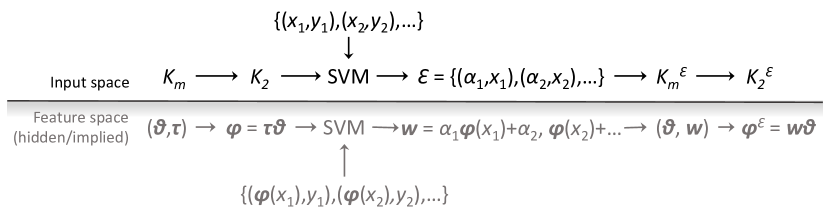
Figure 1: Kernel Pre-training Procedure. Working left to right in input space: (1) start with a kernel $K_{2}$ derived from a free kernel $K_{m}$. (2) Train SVM to obtain $\alpha_{1},\alpha_{2},\ldots$. (3) Using (12) obtain re-weighted kernel $K_{2}^{\mathcal{E}}$ derived from free kernel $K_{m}^{\mathcal{E}}$. The feature space operation implied by each step is shown below the line: (1) start with a feature map ${\mbox{\boldmath$\tau$}}{\mbox{\boldmath$\vartheta$}}({\bf x})$ implied by $K_{2}$. (2) Train SVM to obtain weights ${\bf w}$. (3) Using (12) obtain re-weighted feature map ${\bf w}{\mbox{\boldmath$\vartheta$}}({\bf x})$ implied by $K_{2}^{\mathcal{E}}$. Note that important features (as given by the SVM) $\vartheta_{i}({\bf x})$ will be assigned higher weights $w_{i}$ than less important features.

The utility of this result, as illustrated in figure 1, is that it allows us to take a kernel $K_{2}$ derived from free kernel $K_{m}$, train a (standard $2$-norm) SVM (or similar) equipped with this kernel to obtain (implicitly defined) weights ${\bf w}=\sum_{i}\alpha_{i}{\mbox{\boldmath$\varphi$}}_{2}({\bf x}_{i})=\sum_{i}\alpha_{i}{\mbox{\boldmath$\tau$}}{\mbox{\boldmath$\vartheta$}}({\bf x}_{i})$ (using (7) and (9)), and then use this result to generate a new kernel $K_{2}^{\mathcal{E}}$ derived from the free kernel $K_{m}^{\mathcal{E}}$ using (12)) that gives more weight to important features in feature space (as indicated by large $|w_{i}|$) and less weight to less important features (as indicated by small $|w_{i}|$). The geometric significance of this operation is illustrated in figure 2.

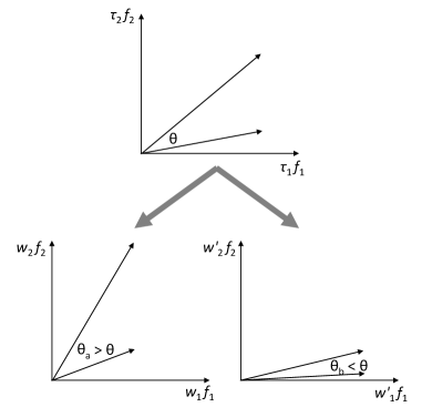
Figure 2: Geometry of kernel re-weighting ($m=2$ case). The upper diagram shows the two vectors ${\mbox{\boldmath$\tau$}}{\mbox{\boldmath$\vartheta$}}({\bf x})$, ${\mbox{\boldmath$\tau$}}{\mbox{\boldmath$\vartheta$}}({\bf x}^{\prime})$ in feature space. The similarity $K({\bf x},{\bf x}^{\prime})$ as measured by $K$ is proportional to $\cos\theta$ as per (2). The lower diagrams show two possible re-weightings. The left-hand case increases the relative weight of feature $2$, resulting in decreased similarity, whilst the right-hand case increases the relative weight of feature $1$, resulting in increased similarity.

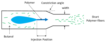
Figure 3: Device geometry for short polymer fibre injection.

Note that at no point in this process do we need to explicitly know the implied feature map or weights. Thus we can directly tune a kernel (covariance) function to fit a given set of problem. As we will show in our results, applying this procedure to Bayesian optimisation where the kernel is tuned to fit some corpus of condensed knowledge results in a significant speed-up due to better fitting of the covariance function.

4 Proposed Algorithm

We now discuss our method for selecting the kernel function. As noted previously, we wish to accelerate Bayesian optimisation by leveraging the additional dataset $\mathcal{D}_{\operatorname{\diamond}}=\{({\bf x}_{{\operatorname{\diamond}}i},y_{{\operatorname{\diamond}}i})|{\bf x}_{{\operatorname{\diamond}}i}\in\mathbb{R}^{n},y_{{\operatorname{\diamond}}i}=f_{\operatorname{\diamond}}({\bf x}_{{\operatorname{\diamond}}i})+\epsilon_{\operatorname{\diamond}}\in\mathbb{Y}\}$, which may be derived for example from relevant patents, handbooks or datasheets. Our proposed algorithm is given in algorithm 2.

Algorithm 2 Bayesian Optimisation with Kernel re-weighting.

0:  $\mathcal{D}_{0},\mathcal{D}_{\operatorname{\diamond}}$, free kernel $K_{m}$.

  Train SVM with $\mathcal{D}_{\operatorname{\diamond}}$ with kernel $K_{2}$ to obtain $\alpha_{{\operatorname{\diamond}}i}$.

  Construct re-weighted covariance function:

$$\begin{array}[]{l}K_{2}^{\mathcal{E}}\left({\bf x},{\bf x}^{\prime}\right)=\sum_{i,j}\alpha_{{\operatorname{\diamond}}i}\alpha_{{\operatorname{\diamond}}j}K_{4}\left({\bf x}_{{\operatorname{\diamond}}i},{\bf x}_{{\operatorname{\diamond}}j},{\bf x},{\bf x}^{\prime}\right)\\ \end{array}$$

  Proceed modelling $f\sim\operatorname{GP}(0,K_{2}^{\mathcal{E}})$.

  for $t=1,2,\ldots,T$ do

     Select test point ${\bf x}_{t}=\operatorname{argmax}_{\bf x}a_{t}({\bf x})$.

     Perform Experiment $y_{t}=f({\bf x}_{t})+\epsilon$.

     Update $\mathcal{D}_{t}:=\mathcal{D}_{t-1}\cup\{({\bf x}_{t},y_{t})\}$.

  end for

The key difference between our proposed algorithm and the standard Bayesian optimisation algorithm (algorithm 1) is that the covariance function $K$ is first re-weighted based on the additional dataset $\mathcal{D}_{\operatorname{\diamond}}$ to ensure that the implied feature weights match those of this dataset before proceeding with the optimisation. Thus we can expect that it will better match the problem at hand in terms of the relative weights it gives to components in feature space.

5 Results

We consider three experiments here, two based on real-world problems and one simulation to highlight the properties of the algorithm.

5.1 Short Polymer Fibres

In this experiment we have tested our algorithm on the real-world application of optimizing short polymer fiber (SPF) to achieve a given (median) target length [8]. This process involves the injection of one polymer into another in a special device [15]. The process is controlled by $3$ geometric parameters (channel width (mm), constriction angle (degree), device position (mm)) and $2$ flow factors (butanol speed (ml/hr), polymer concentration (cm/s)) that parametrise the experiment - see figure 3. Two devices (A and B) were used. Device A is armed by a gear pump and allows for three butanol speeds (86.42, 67.90 and 43.21 cm/s). The newer device B has a lobe pump and allows butonal speed 98, 63 and 48 cm/s. Our goal is to design a new short polymer fiber for Device B that results in a (median) target fibre length of 500$\mu$m.

We write the device parameters as ${\bf x}\in\mathbb{R}^{5}$ and the result of experiments (median fibre length) on each device as $d_{\rm A}({\bf x})$ and $d_{\rm B}({\bf x})$, respectively. Device A has been characterised to give a dataset $\mathcal{D}_{\operatorname{\diamond}}=\{({\bf x}_{{\operatorname{\diamond}}i},y_{{\operatorname{\diamond}}i})|y_{{\operatorname{\diamond}}i}=d_{\rm A}({\bf x}_{{\operatorname{\diamond}}i})\}$ of $163$ input/output pairs. We aim to minimise:

$$\begin{array}[]{l}f\left({\bf x}\right)=\left(d_{\rm B}\left({\bf x}\right)-500\right)^{2}\end{array}$$

noting that $f\neq d_{\rm B}$ (the objective $f$ differs from the function generating $\mathcal{D}_{\operatorname{\diamond}}$, although both relate to fibre length). Device B has been similarly characterised and this grid forms our search space for Bayesian optimisation.

For this experiment we have used a free SE kernel $K_{m}^{\rm se}$. An SVM was trained using $\mathcal{D}_{\operatorname{\diamond}}$ and an SE kernel (hyperparameters $C$ and $\sigma$ were selected to minimise leave-one-out mean-squared-error (LOO-MSE)) to obtain $\mathcal{E}=\{({\bf x}_{{\operatorname{\diamond}}i},\alpha_{{\operatorname{\diamond}}i})\}$. The re-weighted SE kernel $K_{2}^{{\rm se}\mathcal{E}}$ obtained from this was normalised (to ensure good conditioning along the diagonal of ${\bf K}_{t}$) and used in Bayesian optimisation as per algorithm 2. All data was normalised to $[0,1]$ and all experiments were averaged over $40$ repetitions.

We have tested both the EI and GP-UCB acquisition functions. Figure 4 shows the convergence of our proposed algorithm. Also shown for comparison are standard Bayesian optimisation (using a standard SE kernel as our covariance function); and a variant of our algorithm where a kernel mixture model trained on $\mathcal{D}_{\operatorname{\diamond}}$ is used as our covariance function - specifically:

$$\begin{array}[]{l}K\!\left({\bf x},{\bf x}^{\prime}\right)=v_{1}K_{1}\!\left({\bf x},{\bf x}^{\prime}\right)+v_{2}K_{2}\!\left({\bf x},{\bf x}^{\prime}\right)+v_{3}K_{3}\!\left({\bf x},{\bf x}^{\prime}\right)\end{array}$$ (13)

where $K_{1}$ is an SE kernel, $K_{2}$ a Matérn 1/2 kernel, $K_{3}$ a Matérn 3/2 kernel; and $v_{1},v_{2},v_{3}\geq 0$ and all relevant (kernel) hyperparameters are selected to minimise LOO-MSE on $\mathcal{D}_{\operatorname{\diamond}}$. Relevant hyperparameters in Bayesian optimisation ($\nu$ for our method and kernel mixtures, $\nu$ and $\sigma$ for standard Bayesian optimisation) were selected using max-log-likelihood at each iteration. As can be seen our proposed approach outperforms other methods with both GP-UCB and EI acquisition functions.

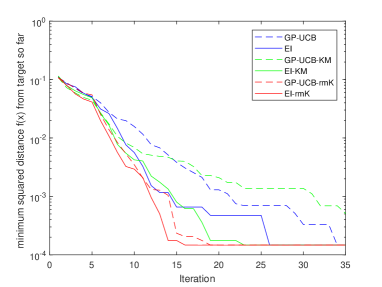
Figure 4: Short Polymer Fibre design. Comparison of algorithms in terms of minimum squared distance from the set target versus iterations. GP-UCB and EI indicate acquisition function used. MK indicates mixture kernel used. rmK indicates our proposed method.

5.2 Aluminium Alloy Design using Thermo-Calc

This experiment considers optimising a new hybrid Aluminium alloy for target yield strength. Designing an alloy is an expensive process. Casting an alloy and then measuring its properties usually takes long time. An alloy has certain phase structures that determine its material properties. For example, phases such as C14LAVES and ALSC3 are known to increase yield strength whilst others such as AL3ZR_D023 and ALLI_B32 reduce the yield strength of the alloy. However a precise function relating the phases to yield strength does not exist. The simulation software Thermo-Calc takes a mixture of component elements as input and computes the phase composition of the resulting alloy. We consider 11 elements as potential constituents of the alloy and 24 phases. We use Thermo-Calc for this computation.

A dataset $\mathcal{D}_{\operatorname{\diamond}}$ of $46$ closely related alloys filed as patents was collected. This dataset consists information about the composition of the elements in the alloy and their yield strength. The phase compositions extracted from Thermo-Calc simulations for various alloy compositions were used to understand the positive or negative contribution of phases to the yield strength of the alloy using linear regression. The weights retrieved for these phases were then used formulate a utility function. Figure 5 shows the regression coefficients for the phases contributing to the yield strength.

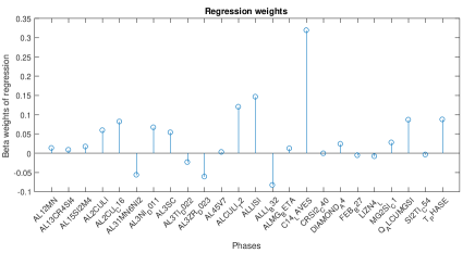
Figure 5: Regression coefficients for 25 phases as determined from patent data.

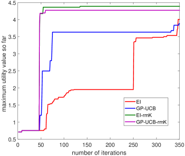
Figure 6: Aluminium alloy design. Comparison of algorithms in terms of maximum utility score versus iterations. GP-UCB and EI indicate acquisition function used. rmK indicates our proposed method.

As in the previous experiment for this experiment we have used a free SE kernel $K_{m}^{\rm se}$. An SVM was trained using $\mathcal{D}_{\operatorname{\diamond}}$ and an SE kernel (hyperparameters $C$ and $\sigma$ were selected to minimise LOO-MSE) to obtain $\mathcal{E}=\{({\bf x}_{{\operatorname{\diamond}}i},\alpha_{{\operatorname{\diamond}}i})\}$. The re-weighted SE kernel $K_{2}^{{\rm se}\mathcal{E}}$ obtained from this was normalised (to ensure good conditioning along the diagonal of ${\bf K}_{t}$) and used in Bayesian optimisation as per algorithm 2. All data was normalised to $[0,1]$.

We have tested both the EI and GP-UCB acquisition functions. Figure 6 shows the convergence of our proposed algorithm compared to standard Bayesian optimisation (using a standard SE kernel as our covariance function). Relevant hyperparameters in Bayesian optimisation ($\nu$ for our method and kernel mixtures, $\nu$ and $\sigma$ for standard Bayesian optimisation) were selected using max-log-likelihood at each iteration. As can be seen our proposed approach outperforms standard Bayesian optimisation by a significant margin for both EI and GP-UCB.

5.3 Simulated Experiment

In this experiment we consider use of kernel re-weighting to incorporate domain knowledge into a kernel design. We aim to minimise the function:

$$\begin{array}[]{l}f\left({\bf x}\right)=\sin\left(5\pi\left\|{\bf x}\right\|_{2}\right)\exp\left(-5\left(\left\|{\bf x}\right\|_{2}-\frac{1}{2}\right)^{2}\right)\end{array}$$

as illustrated in figure 7, where ${\bf x}\in[-1,1]^{2}$. Noting that this function has rotational symmetry we select an additional dataset to exhibit this property, namely:

$$\begin{array}[]{l}\mathbb{D}_{\operatorname{\diamond}}=\left\{\left.\left({\bf x}_{{\operatorname{\diamond}}i},y_{{\operatorname{\diamond}}i}\right)\right|y_{{\operatorname{\diamond}}i}=\left\|{\bf x}_{{\operatorname{\diamond}}i}\right\|_{2}\right\}\end{array}$$

of $100$ vectors, where ${\bf x}_{{\operatorname{\diamond}}i}$ is selected uniformly randomly. Thus $\mathbb{D}_{\operatorname{\diamond}}$ reflects the rotational symmetry of the target optimisation function $f$ but not its form.

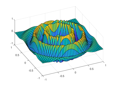
Figure 7: Target optimisation function in experiment 3.

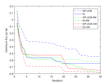
Figure 8: Simulated experiment. Comparison of algorithms in terms of minimum $f({\bf x})$ versus iterations. GP-UCB and EI indicate acquisition function used. MK indicates mixture kernel used. rmK indicates our proposed method.

As for previous experiments we have started with a free SE kernel $K_{m}^{\rm se}$ and re-weighted this by training and SVM on $\mathcal{D}_{\operatorname{\diamond}}$ (using an SE kernel with hyperparameters selected to minimise LOO-MSE) to obtain $\mathcal{E}=\{({\bf x}_{{\operatorname{\diamond}}i},\alpha_{{\operatorname{\diamond}}i})\}$, and constructed the re-weighted (but not normalised in this experiment) SE kernel $K_{2}^{{\rm se}\mathcal{E}}$. However in this case in our Bayesian optimisation we have used the composite kernel:

$$\begin{array}[]{l}K\left({\bf x},{\bf x}^{\prime}\right)=K_{2}^{\rm se}\left(K_{2}^{{\rm se}\mathcal{E}}\left({\bf x},{\bf x}^{\prime}\right)\right)\end{array}$$

which implies a $2$-layer feature map, the first layer being the re-weighted feature map implied by $K_{2}^{{\rm se}\mathcal{E}}$ and the second layer being the standard feature map implied by the SE kernel. All data was normalised to $[0,1]$ and all experiments were averaged over $10$ repetitions.

We have tested both the EI and GP-UCB acquisition functions. Figure 8 shows the convergence of our proposed algorithm compared to standard Bayesian optimisation (using a standard SE kernel) and standard Bayesian optimisation with a kernel mixture model as per our short polymer fibre experiment (13) trained on $\mathcal{D}_{\operatorname{\diamond}}$ used as the covariance function. Curiously in this case, while our method combined with GP-UCB outperforms the alternatives, the results are less clear for our method combined with EI. The precise reason for this will be investigated in future work.

6 Conclusion

In this paper we have presented a novel approach to direct covariance function learning for Bayesian optimisation, focussing on experimental design problems where an existing corpus of condensed knowledge is present. We have based our method on $m$-kernel techniques from reproducing kernel Banach space theory. We have extended Mercer’s theorem to $2q$-kernels; defined free kernel families whose implied feature map is independent of $m$ (and provided a means of constructing them, with examples); shown how the properties of these may be utilised to tune them by effectively modifying the weights in feature space; presented a modified Bayesian optimisation algorithm that makes use of these properties to pre-tune its covariance function on additional data provided; and demonstrated our techniques on two practical optimisation tasks and one simulated optimisation problem, demonstrating the efficacy of our proposed algorithm.

7 Supplementary: Derivation of the $p$-norm SVM Dual - Regression Case

Let $0<p\leq 2$ be dual to $2q$, $q\in\mathbb{N}^{+}$ (i.e. $1/p+1/2q=1$). As defined in the paper, let $\Theta=\{(x_{i},y_{i})|x_{i}\in\mathbb{X},y_{i}\in\mathbb{R}\}$ be a regression training set and let the discriminant function take the standard form:

$$\begin{array}[]{l}g\left(x\right)={\bf w}^{\rm T}{\mbox{\boldmath$\varphi$}}\left(x\right)+b\end{array}$$

where ${\mbox{\boldmath$\varphi$}}:\mathbb{X}\to\mathbb{R}^{d}$ is a feature map implied by the $2q$-kernel $K:\mathbb{X}^{2q}\to\mathbb{R}$. The $p$-norm SVM primal is:

$$\begin{array}[]{l}\begin{array}[]{l}\mathop{\min}\limits_{{\bf w},b,\xi}\frac{1}{p}\left\|{\bf w}\right\|_{p}^{p}+\frac{C}{N}\sum_{i}\xi_{i}\end{array}\\ \begin{array}[]{ll}\mbox{such that:}&{\bf w}^{\rm T}{\mbox{\boldmath$\varphi$}}\left(x_{i}\right)+b-y_{i}\leq\epsilon+\xi_{i}\;\forall i\\ &{\bf w}^{\rm T}{\mbox{\boldmath$\varphi$}}\left(x_{i}\right)+b-y_{i}\geq-\epsilon-\xi_{i}\;\forall i\\ &\xi_{i}\geq 0\;\forall i\\ \end{array}\\ \end{array}$$ (14)

where $C,\epsilon>0$.

Defining Lagrange multipliers ${\bar{\beta}}_{i}\leq 0$, $\beta_{i},\gamma_{i}\geq 0$ for, respectively, the first, second and third constraint sets in the primal (14) (noting that one or both of ${\bar{\beta}}_{i}$ and $\beta_{i}$ must be zero for all $i$, as at most one the first two constraints can be met with equality for any $i$) we obtain the Lagrangian:

$$\!\!\!\!\!\!\begin{array}[]{rl}L&\!\!\!=\frac{1}{p}\left\|{\bf w}\right\|_{p}^{p}+\frac{C}{N}\sum_{i}\xi_{i}-\sum_{i}{\bar{\beta}}_{i}{\bf w}^{\rm T}{\mbox{\boldmath$\varphi$}}\left(x_{i}\right)-\ldots\\ &\ldots-\sum_{i}{\bar{\beta}}_{i}b+\sum_{i}{\bar{\beta}}_{i}y_{i}+\epsilon\sum_{i}{\bar{\beta}}_{i}+\ldots\\ &\ldots+\sum_{i}{\bar{\beta}}_{i}\xi_{i}-\sum_{i}\beta_{i}{\bf w}^{\rm T}{\mbox{\boldmath$\varphi$}}\left(x_{i}\right)-\ldots\\ &\ldots-\sum_{i}\beta_{i}b+\sum_{i}\beta_{i}y_{i}-\epsilon\sum_{i}\beta_{i}-\ldots\\ &\ldots-\sum_{i}\beta_{i}\xi_{i}-\sum_{i}\gamma_{i}\xi_{i}\\ \end{array}\!\!\!\!\!\!$$ (15)

Using the fact that one or both of $\beta_{i}\geq 0$ and ${\bar{\beta}}_{i}\leq 0$ must be zero for all $i$ we see that ${\bar{\beta}}_{i}-\beta_{i}=-|{\bar{\beta}}_{i}+\beta_{i}|$ for all $i$, and hence:

$$\begin{array}[]{l}\nabla_{\bf w}L=\operatorname{sgn}\left({\bf w}\right)\left|{\bf w}\right|^{p-1}-\sum_{i}\left({\bar{\beta}}_{i}+\beta_{i}\right){\mbox{\boldmath$\varphi$}}\left(x_{i}\right)\\ \frac{\partial L}{\partial b}=-\sum_{i}\left({\bar{\beta}}_{i}+\beta_{i}\right)\\ \frac{\partial L}{\partial\xi_{i}}=\frac{C}{N}-\left|{\bar{\beta}}_{i}+\beta_{i}\right|-\gamma_{i}\\ \end{array}$$

where $|{\bf w}|$ and ${\bf w}^{p-1}$ are, respectively, the elementwise absolute value and elementwise power of ${\bf w}$. It follows that, for optimality:

$$\begin{array}[]{l}{\bf w}=\sum_{i}\left({\bar{\beta}}_{i}+\beta_{i}\right)\operatorname{sgn}\left({\mbox{\boldmath$\varphi$}}\left(x_{i}\right)\right)\left|{\mbox{\boldmath$\varphi$}}\left(x_{i}\right)\right|^{2q-1}\\ \sum_{i}\left({\bar{\beta}}_{i}+\beta_{i}\right)=0\\ -\frac{C}{N}\leq\left({\bar{\beta}}_{i}+\beta_{i}\right)\leq\frac{C}{N}\;\forall i\\ \end{array}$$

Defining $\alpha_{i}={\bar{\beta}}_{i}+\beta_{i}$ $\forall i$, substituting into the Lagrangian and using the definition of the $2q$-kernel $K$ (the $2q$-kernel trick) we obtain the dual $p$-norm SVM training problem:

$$\!\!\!\!\!\!\!\!\!\!\!\!\begin{array}[]{l}\begin{array}[]{rl}\mathop{\min}\limits_{\alpha}&\!\!\!\frac{1}{2q}\mathop{\sum}\limits_{i_{1},i_{2},\ldots,i_{2q}}\!\!\!\alpha_{i_{1}}\alpha_{i_{2}}\ldots\alpha_{i_{2q}}K_{i_{1},i_{2},\ldots,i_{2q}}+\ldots\\ &\!\!\!\ldots+\epsilon\sum_{i}\left|\alpha_{i}\right|-\sum_{i}y_{i}\alpha_{i}\end{array}\\ \begin{array}[]{ll}\mbox{such that:}&-\frac{C}{N}\leq\alpha_{i}\leq\frac{C}{N}\;\forall i\\ &\sum_{i}\alpha_{i}=0\\ \end{array}\\ \end{array}\!\!\!\!\!\!\!\!\!\!\!\!$$ (16)

where $K_{i_{1},i_{2},\ldots,i_{2q}}=K(x_{i_{1}},x_{i_{2}},\ldots,x_{i_{2q}})$; and the discriminant function may be written:

$$\begin{array}[]{l}g\left(x\right)=\!\!\!\!\!\mathop{\sum}\limits_{i_{2},\ldots,i_{2q}}\!\!\!\!\!\alpha_{i_{2}}\ldots\alpha_{i_{2q}}K\left(x,x_{i_{2}},\ldots,x_{i_{2q}}\right)+b\end{array}$$ (17)

8 Supplementary: Derivation of the $p$-norm SVM Dual - Binary Classification Case

In the case of binary classification $\Theta=\{(x_{i},y_{i})|x_{i}\in\mathbb{X},y_{i}\in\{-1,+1\}\}$. The discriminant function is:

$$\begin{array}[]{l}g\left(x\right)={\bf w}^{\rm T}{\mbox{\boldmath$\varphi$}}\left(x\right)+b\end{array}$$

where ${\mbox{\boldmath$\varphi$}}:\mathbb{X}\to\mathbb{R}^{d}$ is a feature map implicit in the $2q$-kernel $K:\mathbb{X}^{2q}\to\mathbb{R}$. The $p$-norm SVM primal is:

$$\begin{array}[]{l}\begin{array}[]{l}\mathop{\min}\limits_{{\bf w},b,\xi}\frac{1}{p}\left\|{\bf w}\right\|_{p}^{p}+\frac{C}{N}\sum_{i}\xi_{i}\end{array}\\ \begin{array}[]{ll}\mbox{such that:}&y_{i}\left({\bf w}^{\rm T}{\mbox{\boldmath$\varphi$}}\left(x_{i}\right)+b\right)\geq 1-\xi_{i}\;\forall i\\ &\xi_{i}\geq 0\;\forall i\\ \end{array}\\ \end{array}$$ (18)

Defining Lagrange multipliers ${\bar{\alpha}}_{i},\gamma_{i}\geq 0$ for, respectively, the first and second constraint sets in the primal (18) we obtain the Lagrangian:

$$\!\!\!\!\!\!\begin{array}[]{rl}L&\!\!\!=\frac{1}{p}\left\|{\bf w}\right\|_{p}^{p}+\frac{C}{N}\sum_{i}\xi_{i}-\sum_{i}{\bar{\alpha}}_{i}y_{i}{\bf w}^{\rm T}{\mbox{\boldmath$\varphi$}}\left(x_{i}\right)-\ldots\\ &\ldots-\sum_{i}{\bar{\alpha}}_{i}y_{i}b+\sum_{i}{\bar{\alpha}}_{i}-\sum_{i}{\bar{\alpha}}_{i}\xi_{i}-\sum_{i}\gamma_{i}\xi_{i}\\ \end{array}\!\!\!\!\!\!$$ (19)

and hence:

$$\begin{array}[]{l}\nabla_{\bf w}L=\operatorname{sgn}\left({\bf w}\right)\left|{\bf w}\right|^{p-1}-\sum_{i}{\bar{\alpha}}_{i}y_{i}{\mbox{\boldmath$\varphi$}}\left(x_{i}\right)\\ \frac{\partial L}{\partial b}=\sum_{i}y_{i}{\bar{\alpha}}_{i}\\ \frac{\partial L}{\partial\xi_{i}}=\frac{C}{N}-{\bar{\alpha}}_{i}-\gamma_{i}\\ \end{array}$$

where $|{\bf w}|$ and ${\bf w}^{p-1}$ are, respectively, the elementwise absolute value and elementwise power of ${\bf w}$. It follows that, for optimality:

$$\begin{array}[]{l}{\bf w}=\sum_{i}{\bar{\alpha}}_{i}y_{i}\operatorname{sgn}\left({\mbox{\boldmath$\varphi$}}\left(x_{i}\right)\right)\left|{\mbox{\boldmath$\varphi$}}\left(x_{i}\right)\right|^{2q-1}\\ \sum_{i}y_{i}{\bar{\alpha}}_{i}=0\\ 0\leq{\bar{\alpha}}_{i}\leq\frac{C}{N}\;\forall i\\ \end{array}$$

Defining $\alpha_{i}=y_{i}{\bar{\alpha}}_{i}$ $\forall i$, substituting into the Lagrangian and using the definition of the $2q$-kernel $K$ (the $2q$-kernel trick) we obtain the dual $p$-norm SVM training problem:

$$\!\!\!\!\!\!\!\!\!\!\!\!\begin{array}[]{l}\begin{array}[]{l}\mathop{\min}\limits_{\alpha}\frac{1}{2q}\mathop{\sum}\limits_{i_{1},i_{2},\ldots,i_{2q}}\!\!\!\alpha_{i_{1}}\alpha_{i_{2}}\ldots\alpha_{i_{2q}}K_{i_{1},i_{2},\ldots,i_{2q}}-\sum_{i}y_{i}\alpha_{i}\end{array}\\ \begin{array}[]{ll}\mbox{such that:}&0\leq y_{i}\alpha_{i}\leq\frac{C}{N}\;\forall i\\ &\sum_{i}\alpha_{i}=0\\ \end{array}\\ \end{array}\!\!\!\!\!\!\!\!\!\!\!\!$$ (20)

where $K_{i_{1},i_{2},\ldots,i_{2q}}=K(x_{i_{1}},x_{i_{2}},\ldots,x_{i_{2q}})$; and the discriminant function may be written:

$$\begin{array}[]{l}g\left(x\right)=\!\!\!\!\!\mathop{\sum}\limits_{i_{2},\ldots,i_{2q}}\!\!\!\!\!\alpha_{i_{2}}\ldots\alpha_{i_{2q}}K\left(x,x_{i_{2}},\ldots,x_{i_{2q}}\right)+b\end{array}$$ (21)

9 Supplementary: Proof of Theorem 2

Mercer’s theorem states that [11]:

Theorem 4 (Mercer’s theorem)

Let $K:\mathbb{X}\times\mathbb{X}\to\mathbb{R}$ be a continuous function for which $K(x,x^{\prime})=K(x^{\prime},x)$ and:

$$\begin{array}[]{l}\int_{x,x^{\prime}\in\mathbb{X}}K\left(x,x^{\prime}\right)\psi\left(x\right)\psi\left(x^{\prime}\right)dxdx^{\prime}\geq 0\end{array}$$

for all $\psi:\mathbb{X}\to\mathbb{R}$ satisfying $\int_{x\in\mathbb{X}}|\psi(x)|^{2}dx<\infty$. Then there exists ${\mbox{\boldmath$\varphi$}}:\mathbb{X}\to\mathbb{R}^{d}$, $d\in\mathbb{N}^{+}\cup\{\infty\}$ such that:

$$\begin{array}[]{l}K\left(x,x^{\prime}\right)=\left<{\mbox{\boldmath$\varphi$}}\left(x\right){\mbox{\boldmath$\varphi$}}\left(x^{\prime}\right)\right>\end{array}$$

the series being uniformly and absolutely convergent.

We now prove theorem 3 from the paper:

Proof:

It follows from theorem 4 that for any function $K$ satisfying the conditions given in the theorem the function $L$ defined by $K$ may be written as:

$$\begin{array}[]{l}L\left(z,z^{\prime}\right)=\sum_{n}\nu_{n}\left(z\right)\nu_{n}\left(z^{\prime}\right)\end{array}$$

the series being uniformly and absolutely convergent. Hence:

$$\begin{array}[]{l}K\left(x_{1},\ldots,x_{2q}\right)=\ldots\\ \;\ldots=\sum_{n}\kappa_{n}\left(x_{1},\ldots,x_{q}\right)\kappa_{n}\left(x_{q+1},\ldots,x_{2q}\right)\end{array}$$

where $\kappa_{n}(x_{1},\ldots,x_{q})=\nu_{n}([x_{1},\ldots,x_{q}])$. If $q=1$ this is sufficient to prove the theorem. For the more general case we first note that, using the symmetry of $K$:

$$\!\!\!\!\!\!\begin{array}[]{l}\kappa_{n}\!\left(x_{1},\ldots,x_{i},\ldots,x_{q}\right)\kappa_{n}\!\left(x_{q+1},\ldots,x_{j},\ldots,x_{2q}\right)\\ =\kappa_{n}\!\left(x_{1},\ldots,x_{j},\ldots,x_{q}\right)\kappa_{n}\!\left(x_{q+1},\ldots,x_{i},\ldots,x_{2q}\right)\end{array}\!\!\!\!\!\!$$ (22)

for all $i\leq q<j\in\mathbb{N}_{2q}$ (we denote $\mathbb{N}_{r}=\{1,2,\ldots,r\}$ ). This means that for any product of two such $\kappa_{n}$ functions we may switch arguments between the two $\kappa_{n}$ functions without changing the product. Changing the range of $j$ in the above reasoning to $i<j\leq q$ we see that for all $i<j\in\mathbb{N}_{q}$:

$$\begin{array}[]{l}\kappa_{n}\!\left(x_{1},\ldots,x_{i},\ldots,x_{j}\ldots x_{q}\right)\\ =\kappa_{n}\!\left(x_{1},\ldots,x_{j},\ldots,x_{i}\ldots,x_{q}\right)\end{array}$$ (23)

Next suppose that $\exists n$ such that $\kappa_{n}(a,\ldots,a)=0$ $\forall a\in\mathbb{X}$. Using (22) and (23) we see that $\forall a_{1},\ldots,a_{q}\in\mathbb{X}$:

$$\begin{array}[]{l}\kappa_{n}^{q}\left(a_{1},\ldots,a_{q}\right)=\prod_{i}\kappa_{n}\left(a_{i},\ldots,a_{i}\right)=0\\ \end{array}$$

which implies that $\kappa_{n}$ is trivially zero everywhere and may therefore be removed from the series. Hence we may assume that $\forall n$ there exists $a_{n}\in\mathbb{X}$ such that $\kappa_{n}(a_{n},\ldots,a_{n})\neq 0$. It further follows from (22), (23) that $\forall r<q$:

$$\begin{array}[]{r}\kappa_{n}(x_{1},\ldots,x_{r},x_{r+1},\underbrace{a_{n},\ldots,a_{n}}_{q-r-1})\kappa_{n}\left(a_{n},\ldots,a_{n}\right)=\ldots\\ \ldots=\kappa_{n}(x_{1},\ldots,x_{r},\underbrace{a_{n},\ldots,a_{n}}_{q-r})\kappa_{n}\left(x_{r+1},a_{n},\ldots,a_{n}\right)\end{array}$$

and therefore:

$$\begin{array}[]{r}\kappa_{n}(x_{1},\ldots,x_{r},x_{r+1},\underbrace{a_{n},\ldots,a_{n}}_{q-r-1})=\ldots\\ \ldots=\kappa_{n}(x_{1},\ldots,x_{r},\underbrace{a_{n},\ldots,a_{n}}_{q-r})\phi_{n}\left(x_{r+1}\right)\end{array}$$ (24)

where:

$$\begin{array}[]{l}\phi_{n}\left(x\right)=\frac{\kappa_{n}\left(x,a_{n},\ldots,a_{n}\right)}{\kappa_{n}\left(a_{n},\ldots,a_{n}\right)}\\ \end{array}$$

Recursively applying (24) to $\kappa_{n}(x_{1},\ldots,x_{q})$ it may be seen that:

$$\begin{array}[]{l}\kappa_{n}\left(x_{1},\ldots,x_{q}\right)=\kappa_{n}\left(a_{n},\ldots,a_{n}\right)\phi_{n}\left(x_{1}\right)\ldots\phi_{n}\left(x_{q}\right)\end{array}$$

from which we may deduce that there exists a uniformly and absolutely convergent series representation for $K$:

$$\begin{array}[]{c}K\left(x_{1},\ldots,x_{2q}\right)=\sum_{n}\varphi_{n}\left(x_{1}\right)\ldots\varphi_{n}\left(x_{2q}\right)\end{array}$$

where:

$$\begin{array}[]{l}\varphi_{n}\left(x\right)=\frac{\kappa_{n}\left(x,a_{n},\ldots,a_{n}\right)}{\left|\kappa_{n}\left(a_{n},\ldots,a_{n}\right)\right|^{\frac{q-1}{q}}}\end{array}$$

and $a_{n}\in\{a\in\mathbb{X}\subset\mathbb{R}^{d}|\kappa_{n}(a,\ldots,a)\neq 0\}\neq\emptyset$ $\forall n$, which completes the proof. $\square$

10 Supplementary: Proof of Theorem 3

Proof:

Using the multinomial theorem it may be seen that:

$$\begin{array}[]{l}h\left(\ll\!{\bf x},\ldots,{\bf x}^{\ldots}\!\gg_{m}\right)=\mathop{\sum}\limits_{q\geq 0}\kappa_{q}\ll\!{\bf x},\ldots,{\bf x}^{\ldots}\!\gg_{m}^{q}\\ =\mathop{\sum}\limits_{k_{1},k_{2},\ldots,k_{n}\geq 0}\tau^{2}_{m,k_{\bullet}}\theta_{m,k_{\bullet}}\left({\bf x}\right)\ldots\theta_{m,k_{\bullet}}\left({\bf x}^{\ldots}\right)\\ \end{array}$$

where:

$$\begin{array}[]{l}\theta_{m,k_{\bullet}}\left({\bf x}\right)=\mathop{\prod}\limits_{i\in\mathbb{N}_{n}}\!\left(x_{i}\right)^{k_{i}}\\ \tau_{m,k_{\bullet}}=\sqrt{\kappa_{(\sum_{i}k_{i})}\left(\begin{array}[]{c}\sum_{i}k_{i}\\ k_{1},k_{2},\ldots,k_{n}\\ \end{array}\right)}\\ \end{array}$$

and hence:

$$\begin{array}[]{l}K_{m}\left({\bf x},\ldots{\bf x}^{\ldots}\right)=\;\ll\!{\mbox{\boldmath$\tau$}}^{2},{\mbox{\boldmath$\vartheta$}}\left({\bf x}\right),\ldots,{\mbox{\boldmath$\vartheta$}}\left({\bf x}^{\ldots}\right)\!\gg_{m+1}\end{array}$$

where

$$\begin{array}[]{rl}{\mbox{\boldmath$\vartheta$}}\left({\bf x}\right)&\!\!\!=\mathop{\otimes}\limits_{k_{1},k_{2},\ldots,k_{n}\geq 0}x_{1}^{k_{1}}x_{2}^{k_{2}}\ldots x_{n}^{k_{n}}\\ \end{array}$$

and:

$$\begin{array}[]{rl}{\mbox{\boldmath$\tau$}}&\!\!\!=\mathop{\otimes}\limits_{k_{1},k_{2},\ldots,k_{n}\geq 0}\sqrt{\kappa_{(\sum_{i}k_{i})}\left(\begin{array}[]{c}\sum_{i}k_{i}\\ k_{1},k_{2},\ldots,k_{n}\\ \end{array}\right)}\\ \end{array}$$

are independent of $m$. $\square$

References

- [1] Eric Brochu, Vlad M. Cora, and Nando de Freitas. A tutorial on bayesian optimization of expensive cost functions, with applications to active user modeling and heirarchical reinforcement learning. eprint arXiv:1012.2599, arXiv.org, December 2010.
- [2] Ricky Der and Danial Lee. Large-margin classification in banach spaces. In Proceedings of the JMLR Workshop and Conference 2: AISTATS2007, pages 91–98, 2007.
- [3] Sever S. Dragomir. Semi-inner products and Applications. Hauppauge, New York, 2004.
- [4] Gregory E. Fasshauer, Fred J. Hickernell, and Qi Ye. Solving support vector machines in reproducing kernel banach spaces with positive definite functions. Applied and Computational Harmonic Analysis, 38(1):115–139, 2015.
- [5] José!Miguel Hernández-Lobato, Matthew Hoffman, and Zoubin Ghahramani. Predictive entropy search for efficient global optimization of black-box functions. In NIPS, pages 918–926, 2014.
- [6] Donald R. Jones, Matthias Schonlau, and William J. Welch. Efficient global optimization of expensive black-box functions. Journal of Global optimization, 13(4):455–492, 1998.
- [7] Harold J. Kushner. A new method of locating the maximum point of an arbitrary multipeak curve in the presence of noise. Journal of Basic Engineering, 86(1):97–106, 1964.
- [8] Cheng Li, David Rubín de Celis Leal, Santu Rana, Sunil Gupta, Alessandra Sutti, Stewart Greenhill, Teo Slezak, Murray Height, and Svetha Venkatesh. Rapid bayesian optimisation for synthesis of short polymer fiber materials. Scientific reports, 7(1):5683, 2017.
- [9] Olvi L. Mangasarian. Arbitrary-norm separating plane. Technical Report 97-07, Mathematical Programming, May 1997.
- [10] Olvi L. Mangasarian. Arbitrary-norm separating plane. Operations Research Letters, 24:15–23, 1999.
- [11] James Mercer. Functions of positive and negative type, and their connection with the theory of integral equations. Transactions of the Royal Society of London, 209(A), 1909.
- [12] Carl Edward Rasmussen. Gaussian processes for machine learning. MIT Press, 2006.
- [13] Alexander J. Smola, Zoltán L. Óvári, and Robert C. Williamson. Regularization with dot-product kernels. In T. K. Leen, T. G. Dietterich, and V. Tresp, editors, Advances in Neural Information Processing Systems 13, pages 308–314. MIT Press, 2001.
- [14] Niranjan Srinivas, Andreas Krause, Sham M. Kakade, and Matthias W. Seeger. Information-theoretic regret bounds for gaussian process optimization in the bandit setting. IEEE Transactions on Information Theory, 58(5):3250–3265, May 2012.
- [15] Alessandra Sutti, Mark Kirkland, Paul Collins, and Ross John George. An apparatus for producing nano-bodies: Patent WO 2014134668 A1.
- [16] Haizhang Zhang, Yuesheng Xu, and Jun Zhang. Reproducing kernel banach spaces for machine learning. Journal of Machine Learning Research, 10:2741–2775, 2009.