Radial transport and plasma heating in Jupiter’s magnetodisc

Abstract

The ion temperature of the magnetosphere of Jupiter derived from Galileo PLS data was observed to increase by about an order of magnitude from 10 to 40 Jupiter radii. This suggests the presence of heating sources that counteract the adiabatic cooling effect of expanding plasma. There have been different attempts of explaining this phenomena, including a magnetohydrodynamic (MHD) turbulent heating model which is based on flux tube diffusion [Saur, Astrophys. J. Lett., 602, L137, 2004]. We explore an alternate turbulent heating model based on advection, similar to models commonly used in solar wind heating. Based on spectral analysis of Galileo magnetometer (MAG) data, we find that observed MHD turbulence could potentially provide the required heating to explain some of the increase in plasma temperature. This indicates that advection is a more appropriate way to describe radial transport of plasma in the jovian magnetosphere beyond 10 Jupiter radii.

¡JGR-Space Physics¿

Geophysical Institute, University of Alaska Fairbanks, Fairbanks, Alaska, USA

Chung-Sang Ngcng2@alaska.edu

Jupiter’s observed radial ion temperature profile is found to be consistent with heating by turbulent magnetic field fluctuations.

An advective outflow approach for calculating turbulent heating is reasonable beyond 10 ${\rm R_{J}}$ where transport becomes rapid and dominated by large-scale motion.

The turbulent heating rate density has been recalculated, resulting in much higher values for the region between 10 and 20 ${\rm R_{J}}$ than previously reported. This increase is critical in the calculation of temperature that is consistent with observational data.

1 Introduction

Jupiter’s immense magnetosphere is due to the combination of a strong planetary magnetic field, rapid rotation and an internal plasma source (Kivelson, 2014; Delamere et al., 2015a; Achilleos et al., 2015). Io’s supplies neutral gas to the inner magnetosphere at a rate of roughly 1 ton/second and most of this gas is ionized forming the Io plasma torus (Schneider and Bagenal, 2007). However, the accumulation of plasma mass cannot be sustained due to outward radial plasma transport in the form of a centrifugally-driven flux tube interchange instability in a dipole magnetic field configuration (Ma et al., 2016). As the magnetic field becomes stretched into a magnetodisc configuration, it has been suggested that radial transport is governed by magnetodisc reconnection in the middle and outer magnetosphere (Delamere et al., 2015b). Empirical evidence shows that the plasma must be heated nonadiabatically during the transport process (Bagenal and Delamere, 2011)). For example, in Fig. 12 of (Bagenal and Delamere, 2011)), the quantity $PV^{\gamma}$ is plotted for both the thermal and hot particle populations over the range of 6 to 40 radii of Jupiter ${\rm R_{J}}$ and further, showing that it is far from conserved at Jupiter. In this paper we address nonadiabatic heating with a turbulent heating model based on advective outflow commonly used for solar wind heating (see e.g. Ng et al., 2010a, b, and references therein).

Southwood and Kivelson (1987) showed that if the mass content per unit magnetic flux, $\eta=\int\left(\rho/B\right)ds$ decreases with radial distance (i.e. $\partial\eta/\partial L<0$, where $L$ is the radial distance in the unit of ${\rm R_{J}}$) then the plasma torus is centrifugally unstable. Note that $\rho$ is the mass density and $B$ is the magnetic field strength, with the integral over the path length $ds$ of the magnetic field line along a flux tube. Quantities defined similarly are the flux tube volume per unit of magnetic flux $V=\int ds/B$, and the flux tube integrated number density $N=\int nds$ with $n$ being the number density of particles. Also, if the flux tube entropy, $S=\int\left(p^{1/\gamma}/B\right)ds$, decreases with radial distance, then the torus is unstable. However, the flux tube entropy increases with radial distance due to an ever increasing flux tube volume and because of increasing plasma pressure in the middle and outer magnetosphere (Paranicas et al., 1991; Mauk et al., 2004). In general, if $\partial S/\partial L>0$ then the magnetodisc should be stable to centrifugal interchange motion. Understanding the competing effects of negative flux tube mass content gradients and positive flux tube entropy gradients is key to understanding the nature of radial transport physics.

In the inner magnetosphere (e.g., inside of 9 ${\rm R_{J}}$), the torus exhibits a strong negative flux tube content gradient (Bagenal, 1994). In Fig. 9 of (Bagenal et al., 2016), radial profiles of flux tube content ($NL^{2}$, $\eta$) are plotted from a recent re-analysis of Galileo plasma science instrument (PLS) data. It is shown that beyond 10 ${\rm R_{J}}$, the gradient of these quantities is significantly reduced, which naturally precludes significant diffusion. It is also in this region that the radial transport rates increase significantly. In Fig. 10 of (Bagenal and Delamere, 2011), the empirically-derived radial transport rates and integrated transport times are plotted. It is shown that the integrated transport time from 6 to 10 ${\rm R_{J}}$ is 10 to 40 days, while from 10 ${\rm R_{J}}$ to the outer magnetosphere is on the order of one day with radial outflow speeds $\sim$10s to 100s km/s. Delamere and Bagenal (2010) noted that the radial outflow speed can be comparable to the local Alfvén speed (based on the unperturbed dipole) in the middle to outer magnetosphere, suggesting that the concept of a “planetary wind” analogous to the situation in the solar wind is possible (Kennel and Coroniti, 1977). Alternatively, truncation of Alfvénic communication to the planet can also be achieved via pressure anisotropy (Kivelson and Southwood, 2005; Vogt et al., 2014), allowing for a free (e.g., ballooning-type) outflow. Thus, we suggest that radial transport beyond 10 ${\rm R_{J}}$ is governed by magnetodisc reconnection in an impulsive manner (i.e,. bursty bulk flows) and involving large-scale radial motions of mixed entropy flux tubes (Delamere et al., 2011). Therefore, we suggest that while slow diffusive transport is valid in the inner magnetosphere ($<$ 10 ${\rm R_{J}}$), transport in the middle magnetosphere might be better modeled with large-scale convective inflow/outflow channels.

Saur (2004) considered the possibility of turbulent heating of Jupiter’s magnetodisc (10 to 40 ${\rm R_{J}}$) using a diffusive transport model. The diffusion equation for a dipole geometry is of the form

$$\frac{\partial Y}{\partial t}=L^{2}\frac{\partial}{\partial L}\left(\frac{D_{LL}}{L^{2}}\frac{\partial Y}{\partial L}\right)\sim 0\;,$$ (1)

for quasi steady state, where $L$ is the radial coordinate ($L=R/R_{J}$ where ${\rm R_{J}}$ is the planetary radius) and $Y$ is any conserved quantity during flux tube interchange motion. The conserved quantity for mass is $Y=NL^{2}$, or the total number of ions per unit of magnetic flux. For energy, the flux tube content for a centrifugally confined plasma is $NL^{2}3k_{B}T/2$, with $k_{B}$ being the Boltzmann constant. Following Richardson and Siscoe (1983), the diffusion equation for the flux tube energy is

$$L^{2}\frac{\partial}{\partial L}\left(\frac{D_{LL}}{L^{2}}\frac{3\partial nk_{B}TL^{3+\gamma}}{2\partial L}\right)=-qZR^{2}_{J}L^{3+\gamma}\;,$$ (2)

where $\gamma=2$ is used for a equatorially confined plasma sheet with a hight of $Z\sim 2R_{J}$. The $q$ factor in the right hand side of Eq. (2) is the per volume heating rate, presumably from turbulent heating in this model. Assuming $n=n_{0}L^{-\beta}$, with $\beta\sim 6.6$ from observation, and $D_{LL}=D_{0}L^{\beta}$ at the same time, Eq. (2) can be integrated to obtain an equation for the temperature,

$$T=\left(T_{0}-\frac{F_{E}}{F_{n}}\right)\left(\frac{L}{L_{0}}\right)^{\beta-3-\gamma}+\frac{F_{E}}{F_{n}}\left(\frac{L}{L_{0}}\right)^{-\gamma}+\frac{4\pi\left(3-\beta\right)Z_{0}R^{2}_{J}}{3k_{B}F_{n}L^{-\beta+3+\gamma}}\int^{L}_{L_{0}}dL^{\prime}L^{\prime 2-\beta}\int^{L^{\prime}}_{L_{0}}dL^{\prime\prime}qL^{\prime\prime 1+\gamma}\;,$$ (3)

where $F_{n}$ is the diffusive particle flux at $L=L_{0}=12$ (with a value corresponding to $330$ kg s^-1 used in (Saur, 2004)), $F_{E}$ is the radial energy flux at $L_{0}$ and is treated as a fitting parameter. The heating rate function $q$ calculated in (Saur, 2004) is based on a weak turbulence theory (Ng and Bhattacharjee, 1996) using Galileo data. Based on this $q$ function, Saur (2004) found that the observed increasing plasma temperature profile could be explained through inward diffusive transport of thermal energy of $F_{E}=-2.0$ TW generated in the middle magnetosphere by turbulent heating (e.g., 20-30 ${\rm R_{J}}$) with an outward energy flux at $L=35$.

In reconsidering the turbulent heating process, we have also re-analyzed the heating rate function $q$ as presented in Sections 2.2 and 3. Motivated by the significant difference between our calculation and what was calculated by Saur (2004), we look into Eq. (3) more carefully. We see that the qualitative trend of an increasing temperature resulted from Eq. (3) is in fact not very sensitive to the magnitude of $q$. In fact, the increasing trend is mainly determined by the dependence on $L$ in the first and third terms. In the large $L$ limit, both terms are proportional to $L^{\beta-3-\gamma}$, or $L^{1.6}$ based on parameters used in the paper, and thus are increasing roughly at the same rate as in observed data. The $L^{\beta-3-\gamma}$ dependence is originated from the adiabatic condition as can be inferred also from Eq. (2). In (Saur, 2004), the special case of $q=0$ is considered. For this case, $F_{E}$ has to be chosen as $T_{0}F_{n}$ so that both the first and third terms are identically zero. This would result in a decreasing temperature dependence of $L^{-\gamma}$, or $L^{-2}$, due to the second term. However, for any non-zero $q$ such that $F_{E}\neq T_{0}F_{n}$ exactly, the temperature will be increasing due to the first and the third terms since the second term becomes small for larger $L$. Eq. (3) is therefore not sensitive enough to constrain the magnitude of $q$ based on an observed increasing profile. Nevertheless, turbulence can still play an important role in heating Jupiter’s magnetodisc. As discussed above, it is actually reasonable to approach the heating problem with an advective outflow model, similar to the application in the solar wind heating problem. With this approach, we show in the following sections that the observed heating is consistent with dissipation of turbulent magnetic field fluctuations.

2 Turbulent plasma heating

2.1 Temperature model

A turbulent heating model based on advective transport can be derived from the heating equation of an ideal gas,

$$\frac{3}{2}n^{5/3}\frac{d}{dt}\left(pn^{-5/3}\right)=q\,,$$

where $n$ is the number density, $p=nk_{B}T$ is the pressure, and $q$ is the heating rate per volume. The time derivative is taken as the convective derivative $d/dt=\partial/\partial t+{\bf v}\cdot{\bf\nabla}={\bf v}\cdot{\bf\nabla}$ for steady state, where ${\bf v}$ is the advective velocity, with a magnitude $v$, so that

$$v\frac{d}{dr}\left(k_{B}Tn^{-2/3}\right)=\frac{2}{3}n^{-5/3}q\,.$$

Using $r=LR_{J}$ and assuming $n\propto L^{-\beta}$ as in (Saur, 2004), this becomes

$$\frac{dT}{dL}=-\frac{2\beta T}{3L}+\frac{2R_{J}}{3k_{B}nv}q\,.$$

The advective velocity is assumed to carry out in steady state the mass loading rate $\dot{M}$ (taken to be 330 kg/s). Note that due to magnetic flux conservation there must be return flow from the outer region back to the inner region. However, since in MHD average velocity is weighted by mass density, the outflow carrying mass dominates in the average over the return flow after mass is dumped in the outer magnetosphere. Moreover, the outflow with higher density also contributes more in the averaging of ion temperature. Therefore we assume in this paper that the increase in ion temperature is mainly due to the heating following the outflow. If the plasma is assumed to be confined to a disk thickness $\sim HR_{J}$, where $H$ is the scale height, then $\dot{M}\sim 2\pi LHR_{J}^{2}m_{i}nv$ so that $nv\propto L^{-1}$ and the temperature equation can then be written as

$$\frac{dT}{dL}=-\frac{2\beta T}{3L}+c_{1}L^{\alpha}q\,,$$ (4)

where $\alpha$ and $c_{1}$ are parameters determined by confinement geometries. In the case where plasma is confined to a disk $\alpha=1$ and $c_{1}$ can be written as

$$c_{1}=\frac{2}{3}\frac{R_{J}^{3}2\pi m_{i}H}{\dot{M}k_{B}}\,,$$

so that it is about $2\times 10^{19}~{}{\rm Km^{3}}/{\rm W}$. Eq. (4) can then be solved for temperature,

$$T=T_{0}\left(\frac{L}{L_{0}}\right)^{-2\beta/3}+c_{1}\left(\frac{L}{L_{0}}\right)^{-2\beta/3}\int_{L_{0}}^{L}q(L^{\prime})\frac{L^{\prime\alpha+2\beta/3}}{L_{0}^{2\beta/3}}dL^{\prime}\,.$$ (5)

The first term in this temperature equation satisfies the adiabatic condition in the absence of heating and depicts cooling of the expanding plasma. The second term describes the effect of turbulent heating.

2.2 Plasma turbulent heating model

In a turbulent theory (Kolmogorov, 1941; Iroshnikov, 1963; Kraichnan, 1965; Ng and Bhattacharjee, 1996), the energy cascade rate from one scale to another is given by

$$\epsilon\sim\frac{E_{k}}{\tau}\,,$$

where the $E_{k}$ is the energy and $\tau$ is the transfer time scale at a spatial scale (wavenumber) $k$. Assuming equipartition between kinetic and magnetic energy in MHD turbulence, we have

$$E_{k}\sim 2\frac{\delta B_{\perp}^{2}}{2\mu_{0}\rho}\,,$$

where $\delta B_{\perp}$ is the magnitude of magnetic field fluctuations at scale $k$ perpendicular to the large scale magnetic field. The dispersion relation of wave packets is $\omega\sim k_{\parallel}v_{A}\sim v_{A}/\lambda_{\parallel}$, where $v_{A}$ is the Alfvén speed and $\lambda_{\parallel}$ is the spatial scale parallel to the large scale magnetic field at scale $k$. The displacement $\delta r$ of the field per each interaction can be estimated from the Walen relation (also valid for nonlinear Alfvén waves)

$$\frac{\delta u_{\perp}}{v_{A}}=\frac{\delta r\delta t}{\delta t\lambda_{\parallel}}=\frac{\delta B_{\perp}}{B_{0}}\,,$$

where $\delta t$ is the interaction time and $B_{0}$ is the magnitude of the large scale magnetic field, so that

$$\delta r=\frac{\delta B_{\perp}}{B_{0}}\lambda_{\parallel}\,.$$

The fractional change as compared with the perpendicular scale $\lambda_{\perp}$ of the wave packet is

$$\chi\sim\frac{\delta r}{\lambda_{\perp}}\sim\frac{\delta B_{\perp}}{B_{0}}\frac{\lambda_{\parallel}}{\lambda_{\perp}}\sim\frac{\delta B_{\perp}}{B_{0}}\frac{k_{\perp}}{k_{\parallel}}\,.$$

When $\chi\ll 1$, the wave packets are only slightly altered by the distortion of the magnetic field line in one interaction time and thus for weak turbulence many random interactions are required to induce a fractional change or order unity (Ng and Bhattacharjee, 1996). The turbulent cascade time scale is therefore

$$\tau\sim\chi^{-2}\frac{1}{k_{\parallel}v_{A}}\sim\sqrt{\mu_{0}\rho}\frac{B_{0}}{\delta B_{\perp}^{2}}\frac{k_{\parallel}}{k_{\perp}^{2}}\,.$$

Then the turbulent heating rate of plasma can be found from the energy cascade rate

$$q_{\rm MHD-weak}\sim\epsilon\rho\sim\frac{1}{\sqrt{\mu_{0}^{3}\rho}}\frac{\delta B_{\perp}^{4}}{B_{0}}\frac{k_{\perp}^{2}}{k_{\parallel}}\,.$$ (6)

In the strong turbulence limit $\chi\rightarrow 1$ and the Walen relationship becomes $k_{\parallel}v_{A}\rightarrow k_{\perp}\delta u_{\perp}$ so that the turbulent cascade time becomes

$$\tau\sim\frac{1}{k_{\perp}\delta u_{\perp}}\sim\frac{\sqrt{\mu_{0}\rho}}{k_{\perp}\delta B_{\perp}}\,,$$

and the heating rate density is given by

$$q_{\rm MHD-strong}\sim\frac{\delta B_{\perp}^{3}k_{\perp}}{\sqrt{\mu_{0}^{3}\rho}}\,.$$ (7)

Spectral indices corresponding to cascade rates based on Eq. (6) or Eq. (7) are $-2$ and $-5/3$ respectively. As discussed in more detail later, observed spectral indices are mostly between these two values, as shown in Fig. 2. In this paper, we will present calculations based on Eq. (6) only. We have also used Eq. (7) in calculations which result in stronger heating but with qualitatively similar trend. Therefore, we will not repeat the discussion for that case here.

3 Data analysis

Turbulent heating processes are estimated from Galileo magnetometer (MAG) (Kivelson et al., 1992) observations in the jovian magnetosphere. The magnetic field was analyzed in spherical Jupiter centered solar magnetic coordinates. The radial coordinate $\widehat{\boldsymbol{e}}_{r}$ is in the direction away from the planet. Azimuthal coordinate is in the direction of corotation such that $\widehat{\boldsymbol{e}}_{\phi}$ is perpendicular to the plane defined by $\widehat{\boldsymbol{e}}_{\Omega}$ and $\widehat{\boldsymbol{e}}_{r}$ where $\widehat{\boldsymbol{e}}_{\Omega}$ is in the direction of the magnetic dipole axis, and $\widehat{\boldsymbol{e}}_{\theta}=\widehat{\boldsymbol{e}}_{\phi}\times\widehat{\boldsymbol{e}}_{r}$ completes the right hand coordinate system.

For this analysis two-hour windows with at least 600 measurements (i.e. average $\Delta t\leq 12\,{\rm s}$) were selected. Linear interpolation was then used to break the time series into regular sampling intervals. The window mean magnetic field $\boldsymbol{B}_{0}(t)$ was chosen as a 2000 s moving average, so that the size of the analyzed window is a little over 5000 s (with small variations depending on the original sampling rate).

Perturbation of the magnetic field is then calculated as $\delta\boldsymbol{B}(t)=\boldsymbol{B}(t)-\boldsymbol{B}_{0}(t)$, and perpendicular fluctuations of the field as $\delta\boldsymbol{B}(t)_{\perp}=\delta\boldsymbol{B}(t)-\delta\boldsymbol{B}(t)_{\parallel}$, where $\delta\boldsymbol{B}(t)_{\parallel}$ is the component of the perturbation in the direction of $\boldsymbol{B}_{0}(t)$. The power spectrum of the vector components of $\delta\boldsymbol{B}(t)_{\perp}$ was then estimated as (Tao et al., 2015)

$$P(f)=\frac{2}{N\Delta t}\sum_{i=1}^{N}\Delta t\left|W_{i}(t_{i},f)\right|^{2}\,,$$

with the wavelet period of $(1.03f)^{-1}$ (Farge, 1992; Torrence and Compo, 1998). The total power spectrum of the perpendicular fluctuation was calculated as a square root of the sum of squares of the component power spectra.

The heating rate density was calculated from the slope of the power spectrum of $\delta\boldsymbol{B}(t)_{\perp}$ in the range of frequencies between $3\times 10^{-3}$ Hz and $3\times 10^{-2}$ Hz or half of the ion gyro frequency $f_{i}=ZeB_{0}/m_{i}$ (whichever is smaller). Using conservation of energy $\delta b^{2}\sim P(f)f$ (Leamon et al., 1999) and Eq. (6) the heating rate density can be calculated as

$$q=\frac{1}{\sqrt{\mu_{0}^{3}\rho}}\frac{\delta b^{4}}{B_{0}}\frac{k_{\perp}^{2}}{k_{\parallel}}\,,$$ (8)

where $k_{\parallel}=(HR_{J})^{-1}$, $k_{\perp}=2\pi f/v_{\rm rel}\sin(\theta_{vB})$ (von Papen et al., 2014) with $v_{\rm rel}$ being the magnitude of the flow velocity in the spacecraft frame and $\theta_{vB}$ being the angle between the flow velocity and $\boldsymbol{B}_{0}$, and $B_{0}$ is the magnitude of the time average of magnetic field over the analyzed window. Empirical radial profiles of scale height $H$ and plasma density in the magnetodisc is given by Bagenal and Delamere (2011). Plasma in the jovian magnetosphere is composed mainly of oxygen and sulfur ions, expelled by volcanic activity on the moon Io. The average ion mass used in this analysis is taken to be 22 AMU. The heating rate density was calculated and averaged over the analyzed frequency range. An example of this calculation is shown in Figure 1. For this analysis we use samples where the heating rate density varies less than a factor of 15 over the whole range, and we limit the relative magnetic field fluctuations to $\delta B_{\perp}<0.2B_{0}$ with the intent of removing larger fluctuations that could potentially be associated with spatial structures.

Employing the selection criteria described above, 108 samples were chosen. A histogram of the slopes of power spectra in the analyzed frequency range of the selected samples is presented in Figure 2, with the peak of values between $-1.5$ and $-2$. Figure 3 shows the turbulent heating rate density between 10 and 35 ${\rm R_{J}}$. A power law fit to heating rate density averaged over 2${\rm R_{J}}$ bins using a geometric mean has the form $q\approx(1.2\times 10^{-14})L^{-0.57}$ W$/$m³ (blue curve).

Note that our heating rate density is significantly different from what is shown in Saur (2004), especially for $L<20$. This is due to the fact that Saur (2004) imposes an absolute limit of the magnetic fluctuations ($\delta B_{\perp}<0.7\,{\rm nT}$) for all range of $L$ (Saur et al., 2002), as compared with our relative limit of $\delta B_{\perp}<0.2B_{0}$. This means that for smaller $L$, Saur (2004) excludes more data with stronger fluctuations than our calculation since $B_{0}$ is larger for smaller $L$, and thus results in smaller heating rate density. This difference is important since the temperature calculation presented below depends critically on our new calculation. If a much smaller heating rate density is used in the temperature calculation, the temperature would not be increasing fast enough to be consistent with observations.

Using the heating rate density fit and Eq. (5), temperature can then be calculated as a function of the radial distance as shown in Figure 4 (blue curve). Here the initial temperature $T_{0}$ was taken to be $1.7\times 10^{6}$ K ($\sim$150 eV) from the empirical temperature profile of Bagenal and Delamere (2011) (black dashed curve). Within a factor of two, the profiles are in general agreement.

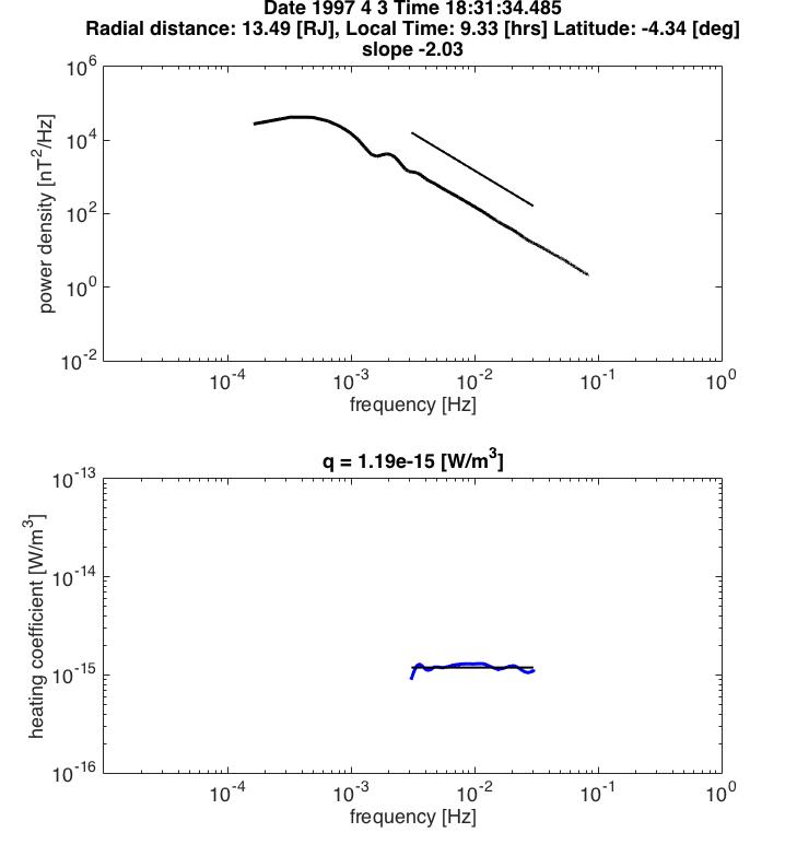
Figure 1: An example of the calculation of the heating rate density (bottom panel) from a power spectrum (top panel). A weak turbulence model is used to calculate the heating rate density in the frequency subrange [$3\times 10^{-3}$, $3\times 10^{-2}$] Hz. The straight line in the top panel is to indicate a slope of $-2$ over this range as expected from the weak turbulence model. The straight line in the bottom panel indicates an average value.

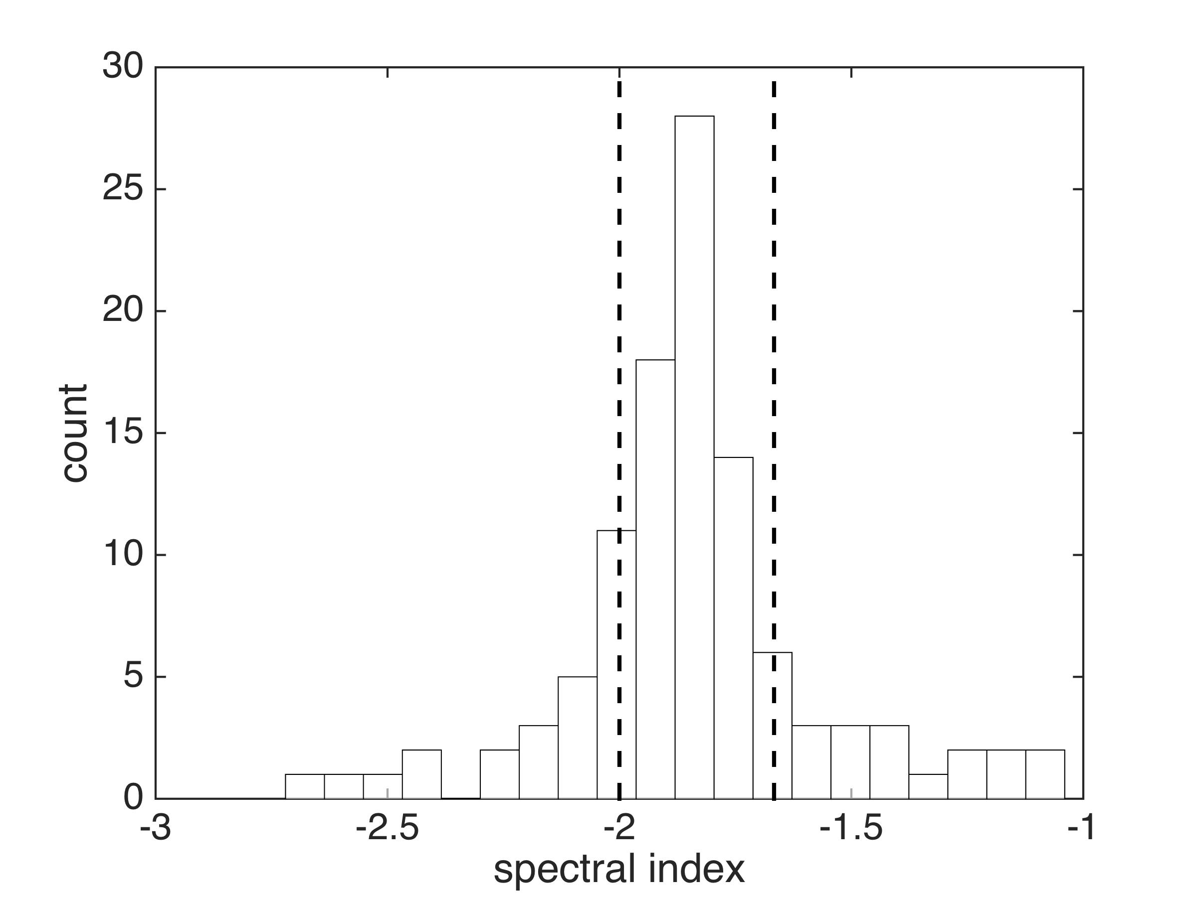
Figure 2: Histogram of slopes of power spectra. The majority of values lie between $-5/3$ and $-2$ (represented by dashed lines).

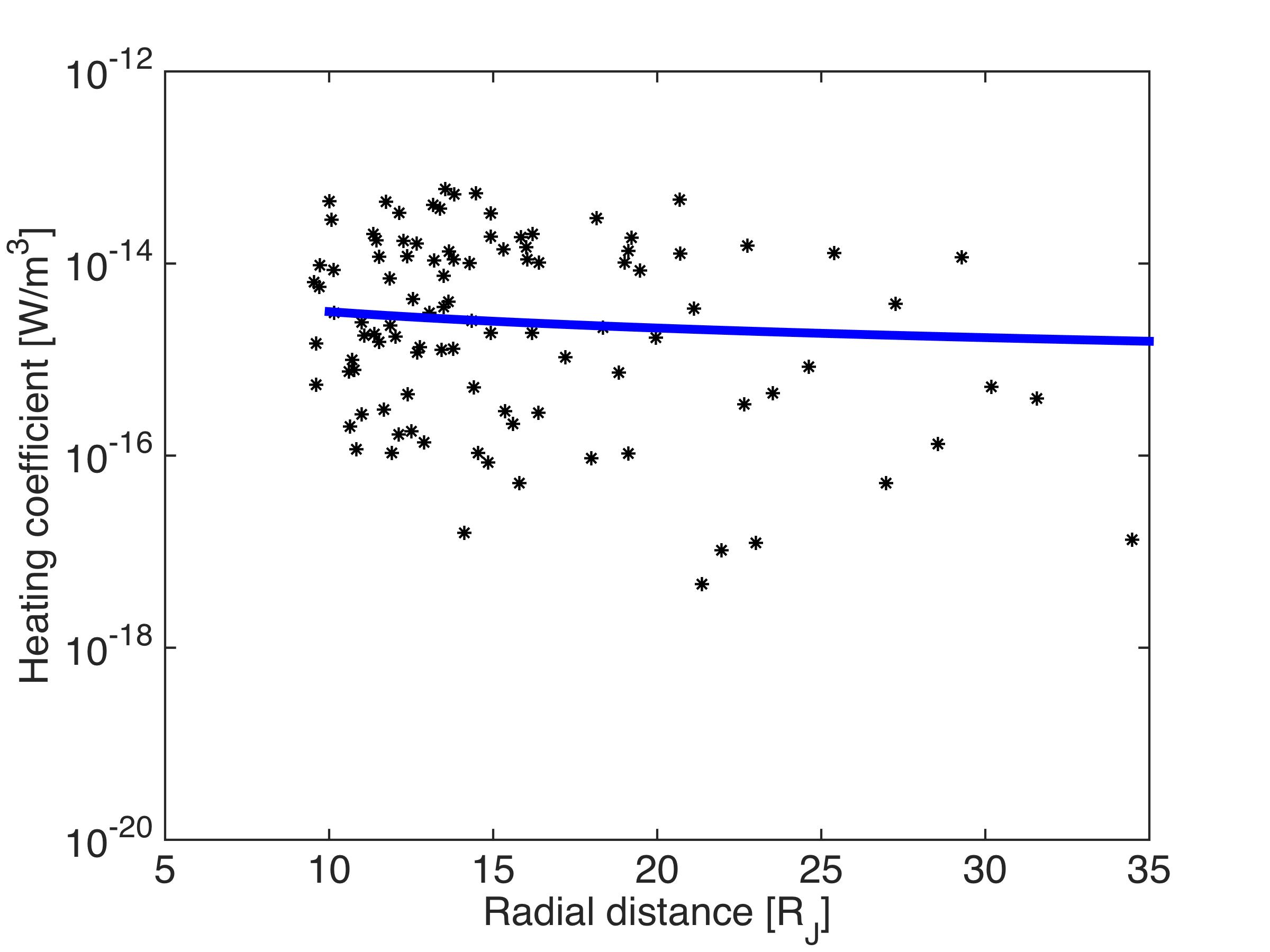
Figure 3: Heating rate density as a function of the radial distance in Jupiter radii. The blue line depicts a power law, $q~{}\approx~{}(1.2\times 10^{-14})L^{-0.57}$ W$/$m³, fit to the data averaged in $1~{}{\rm R_{J}}$ bins.

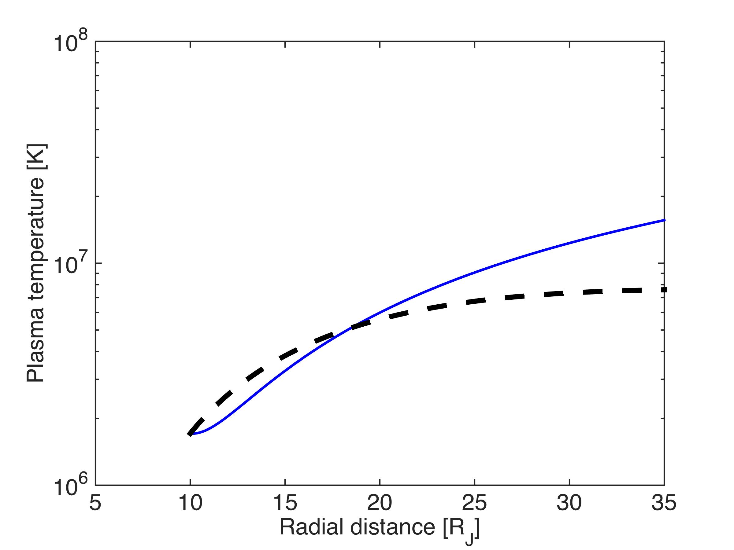
Figure 4: Temperature profile (blue line) calculated from Eq. 5, using the calculated turbulent heating rate density shown in Figure 3. Black dashed line represents a temperature profile from Bagenal and Delamere (2011).

4 Discussion

Understanding the physical mechanisms that lead to plasma heating in the giant magnetospheres is a decades-long conundrum. Magnetodisc equilibrium models (e.g., (Caudal, 1986)) have demonstrated the role of plasma pressure and even pressure anisotropy in radial stress balance (Paranicas et al., 1991). An obvious energy source is planetary rotation and the centrifugal potential (Vogt et al., 2014), though the solar wind can also contribute (Bagenal and Delamere, 2011). In this paper, we have explored the role of turbulent magnetic fields as a plasma heating mechanism, following Saur (2004). However, we have adopted an alternative transport model based on advective outflow of magnetodisc plasma beyond 10 ${\rm R_{J}}$, showing that the heating rate density due to turbulent dissipation is sufficient to account for Jupiter’s observed radial ion temperature profile.

Recent observations by the Juno’s Jupiter Energetic-particle Detector Instrument (JEDI) (Mauk et al., 2017a, b) suggest that auroral electrons at Jupiter are dominated by power-law distributions. These broad-band energy distributions are suggestive of energization by dispersive scale Alfvén waves (e.g. Chaston et al., 2002, 2003; Wing et al., 2013) often attributed to Alfvénic aurora at Earth where Alfvénic energy may reach dispersive scales via a turbulent cascade (Chaston et al., 2008). In this case, we infer a connection between high latitude acceleration by, e.g., inertial Alfvén waves and the observation of kinetic Alfvén waves (i.e., strong magnetic field fluctuations) in the equatorial magnetodisc. Alfvén waves on these dispersive scale lengths (Lysak and Lotko, 1996) are capable of converting significant Poynting flux to electron kinetic energy (precipitation) (Chaston et al., 2002; Wright et al., 2003; Damiano et al., 2007). Likewise, following Saur (2004), we infer that kinetic Alfvén waves in the magnetodisc can serve as the catalyst in ion heating (Johnson and Cheng, 2001) to complete the turbulent cascade.

An interesting difference between Jupiter and Earth is the role of multiple resonant cavities due to density variations along the magnetic field line (Delamere, 2016). Wave transmission to high latitude is a function of parallel wavelength, and (Wright and Schwartz, 1989; Delamere et al., 2003; Hess et al., 2010) showed that significant reflection can occur for perturbations associated with the Io-Jupiter interaction. The non-linear interaction between counter propagating waves leads to a turbulent cascade. We suggest here that resonant cavities could inhibit steady-state magnetosphere-ionosphere coupling currents and, in fact, promote turbulence.

An additional consideration for the middle and outer magnetosphere are the long Alfvén travel times. Bagenal (2007) showed that travel times can approach the order of one hour, which is a non-negligible fraction of the planetary rotation period ($\sim$10 hr). If steady M-I coupling currents are prohibited due to the inability of the system to promptly respond to fluctuations (driven by, for example, local time variations), then M-I decoupling is mandatory. Parallel electric fields facilitate decoupling by breaking the frozen-in condition, and we note that parallel electric fields are an inherent property of kinetic/inertial Alfvén waves.

Jupiter is certainly not unique. Turbulent heating can account for magnetodisc heating at Saturn too. Kaminker et al. (2017), von Papen et al. (2014), and von Papen and Saur (2016) showed that magnetic field fluctuations measured by the Cassini magnetometer (MAG) instrument are consistent with the requisite turbulent heating rate density (Bagenal and Delamere, 2011). Using the 1s-average MAG data, Kaminker et al. (2017) compared the heating rate density in both the inertial subrange (MHD scale) and the dissipation scale (kinetic scale) and found that the kinetic scale heating was typically larger. An energy-conserving cascade would predict equal values in both subranges, so the question remains whether energy could be injected at the kinetic scale via, for example, magnetodisc reconnection (Delamere et al., 2015b). A similar analysis that resolves the kinetic time scale using Juno data should be conducted in future studies.

5 Summary

We have analyzed Galileo magnetometer data to investigate plasma heating by turbulent magnetic field fluctuations using an advective transport model. We summarize our findings as follows:

• Our advective outflow model for investigating turbulent heating (e.g., appropriate for the solar wind) is different from the previous studies. Saur (2004) used a diffusive transport model. We argue that an advective outflow approach is reasonable beyond 10 ${\rm R_{J}}$ where transport becomes rapid and dominated by large-scale motion.

• We re-calculate the heating rate density and obtain much higher values for $L<20$ than what is used in Saur (2004). This increase is critical in the calculation of temperature that is consistent with observation data.

• Using an inner boundary at 10 ${\rm R_{J}}$ and specifying an inner boundary temperature (150 eV), we find that Jupiter’s radial ion temperature profile is consistent with heating by turbulent magnetic field fluctuations.

• Turbulence appears to be ubiquitous in the giant magnetospheres and could have significant implications for magnetosphere-ionosphere coupling and auroral processes.