Stealing Hyperparameters in Machine Learning
Abstract
Hyperparameters are critical in machine learning, as different hyperparameters often result in models with significantly different performance. Hyperparameters may be deemed confidential because of their commercial value and the confidentiality of the proprietary algorithms that the learner uses to learn them. In this work, we propose attacks on stealing the hyperparameters that are learnt by a learner. We call our attacks hyperparameter stealing attacks. Our attacks are applicable to a variety of popular machine learning algorithms such as ridge regression, logistic regression, support vector machine, and neural network. We evaluate the effectiveness of our attacks both theoretically and empirically. For instance, we evaluate our attacks on Amazon Machine Learning. Our results demonstrate that our attacks can accurately steal hyperparameters. We also study countermeasures. Our results highlight the need for new defenses against our hyperparameter stealing attacks for certain machine learning algorithms.
I Introduction
Many popular supervised machine learning (ML) algorithms–such as ridge regression (RR) [19] , logistic regression (LR) [20], support vector machine (SVM) [13], and neural network (NN) [16]–learn the parameters in a model via minimizing an objective function, which is often in the form of loss function + regularization term. Loss function characterizes how well the model performs over the training dataset, regularization term is used to prevent overfitting [7], and balances between the two. Conventionally, is called hyperparameter. Note that there could be multiple hyperparameters if the ML algorithm adopts multiple regularization terms. Different ML algorithms use different loss functions and/or regularization terms.
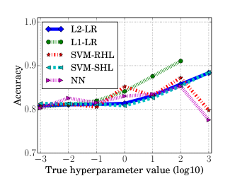
Hyperparameters are critical for ML algorithms. For the same training dataset, with different hyperparameters, an ML algorithm might learn models that have significantly different performance on the testing dataset, e.g., see our experimental results about the impact of hyperparameters on different ML classifiers in Figure 16 in the Appendix. Moreover, hyperparameters are often learnt through a computationally expensive cross-validation process, which may be implemented by proprietary algorithms that could vary across learners. Therefore, hyperparameters may be deemed confidential.
Our work: In this work, we formulate the research problem of stealing hyperparameters in machine learning, and we provide the first systematic study on hyperparameter stealing attacks as well as their defenses.
Hyperparameter stealing attacks. We adopt a threat model in which an attacker knows the training dataset, the ML algorithm (characterized by an objective function), and (optionally) the learnt model parameters. Our threat model is motivated by the emerging machine-learning-as-a-service (MLaaS) cloud platforms, e.g., Amazon Machine Learning [1] and Microsoft Azure Machine Learning [25], in which the attacker could be a user of an MLaaS platform. When the model parameters are unknown, the attacker can use model parameter stealing attacks [54] to learn them. As a first step towards studying the security of hyperparameters, we focus on hyperparameters that are used to balance between the loss function and the regularization terms in the objective function. Many popular ML algorithms–such as ridge regression, logistic regression, and SVM (please refer to Table I for more ML algorithms)–rely on such hyperparameters. It would be an interesting future work to study the security of hyperparameters for other ML algorithms, e.g., the hyperparameter for NN, as well as network architecture, dropout rate [49], and mini-batch size for deep neural networks. However, as we will demonstrate in our experiments, an attacker (e.g., user of an MLaaS platform) can already significantly financially benefit from stealing the hyperparameters in the objective function.
We make a key observation that the model parameters learnt by an ML algorithm are often minima of the corresponding objective function. Roughly speaking, a data point is a minimum of an objective function if the objective function has larger values at the nearby data points. This implies that the gradient of the objective function at the model parameters is close to ( is a vector whose entries are all 0). Our attacks are based on this key observation. First, we propose a general attack framework to steal hyperparameters. Specifically, in our framework, we compute the gradient of the objective function at the model parameters and set it to , which gives us a system of linear equations about the hyperparameters. This linear system is overdetermined since the number of equations (i.e., the number of model parameters) is usually larger than the number of unknown variables (i.e., hyperparameters). Therefore, we leverage the linear least square method [30], a widely used method to derive an approximate solution of an overdetermined system, to estimate the hyperparameters. Second, we demonstrate how we can apply our framework to steal hyperparameters for a variety of ML algorithms.
Theoretical and empirical evaluations. We evaluate our attacks both theoretically and empirically. Theoretically, we show that 1) when the learnt model parameters are an exact minimum of the objective function, our attacks can obtain the exact hyperparameters; and 2) when the model parameters deviate from their closest minimum of the objective function with a small difference, then our estimation error is a linear function of the difference. Empirically, we evaluate the effectiveness of our attacks using six real-world datasets. Our results demonstrate that our attacks can accurately estimate the hyperparameters on all datasets for various ML algorithms. For instance, for various regression algorithms, the relative estimation errors are less than on the datasets.
Moreover, via simulations and evaluations on Amazon Machine Learning, we show that a user can use our attacks to learn a model via MLaaS with much less economical costs, while not sacrificing the model’s testing performance. Specifically, the user samples a small fraction of the training dataset, learns model parameters via MLaaS, steals the hyperparameters using our attacks, and re-learns model parameters using the entire training dataset and the stolen hyperparameters via MLaaS.
Rounding as a defense. One natural defense against our attacks is to round model parameters, so attackers obtain obfuscated model parameters. We note that rounding was proposed to obfuscate confidence scores of model predictions to mitigate model inversion attacks [14] and model stealing attacks [54]. We evaluate the effectiveness of rounding using the six real-world datasets.
First, our results show that rounding increases the relative estimation errors of our attacks, which is consistent with our theoretical evaluation. However, for some ML algorithms, our attacks are still effective. For instance, for LASSO (a popular regression algorithm) [53], the relative estimation errors are still less than around even if we round the model parameters to one decimal. Our results highlight the need to develop new countermeasures for hyperparameter stealing attacks. Second, since different ML algorithms use different regularization terms, one natural question is which regularization term has better security property. Our results demonstrate that regularization term can more effectively defend against our attacks than regularization term using rounding. This implies that an ML algorithm should use regularization in terms of security against hyperparameter stealing attacks. Third, we also compare different loss functions in terms of their security property, and we observe that cross entropy loss and square hinge loss can more effectively defend against our attacks than regular hinge loss using rounding. The cross-entropy loss function is adopted by logistic regression [20], while square and regular hinge loss functions are adopted by support vector machine and its variants [21].
In summary, our contributions are as follows:
-
We provide the first study on hyperparameter stealing attacks to machine learning. We propose a general attack framework to steal the hyperparameters in the objective functions.
-
We evaluate our attacks both theoretically and empirically. Our empirical evaluations on several real-world datasets demonstrate that our attacks can accurately estimate hyperparameters for various ML algorithms. We also show the success of our attacks on Amazon Machine Learning.
-
We evaluate rounding model parameters as a defense against our attacks. Our empirical evaluation results show that our attacks are still effective for certain ML algorithms, highlighting the need for new countermeasures. We also compare different regularization terms and different loss functions in terms of their security against our attacks.
II Related Work
Existing attacks to ML can be roughly classified into four categories: poisoning attacks, evasion attacks, model inversion attacks, and model extraction attacks. Poisoning attacks and evasion attacks are also called causative attacks and exploratory attacks [2], respectively. Our hyperparameter stealing attacks are orthogonal to these attacks.
Poisoning attacks: In poisoning attacks, an attacker aims to pollute the training dataset such that the learner produces a bad classifier, which would mislabel malicious content or activities generated by the attacker at testing time. In particular, the attacker could insert new instances, edit existing instances, or remove existing instances in the training dataset [38]. Existing studies have demonstrated poisoning attacks to worm signature generators [34, 41, 35], spam filters [31, 32], anomaly detectors [43, 24], SVMs [5], face recognition methods [4], as well as recommender systems [27, 57].
Evasion attacks: In these attacks [33, 22, 3, 51, 52, 17, 26, 23, 37, 56, 9, 44, 28, 36], an attacker aims to inject carefully crafted noise into a testing instance (e.g., an email spam, a social spam, a malware, or a face image) such that the classifier predicts a different label for the instance. The injected noise often preserves the semantics of the original instance (e.g., a malware with injected noise preserves its malicious behavior) [51, 56], is human imperceptible [52, 17, 37, 28], or is physically realizable [9, 44]. For instance, Xu et al. [56] proposed a general evasion attack to search for a malware variant that preserves the malicious behavior of the malware but is classified as benign by the classifier (e.g., PDFrate [47] or Hidost [50]). Szegedy et al. [52] observed that deep neural networks would misclassify an image after we inject a small amount of noise that is imperceptible to human. Sharif et al. [44] showed that an attacker can inject human-imperceptible noise to a face image to evade recognition or impersonate another individual, and the noise can be physically realized by the attacker wearing a pair of customized eyeglass frames. Moreover, evasion attacks can be even black-box, i.e., when the attacker does not know the classification model. This is because an adversarial example optimized for one model is highly likely to be effective for other models, which is known as transferability [52, 28, 36].
We note that Papernot et al. [39] proposed a distillation technique to defend against evasion attacks to deep neural networks. However, Carlini and Wagner [10] demonstrated that this distillation technique is not as secure to new evasion attacks as we thought. Cao and Gong [8] found that adversarial examples, especially those generated by the attacks proposed by Carlini and Wagner, are close to the classification boundary. Based on the observation, they proposed region-based classification, which ensembles information in the neighborhoods around a testing example (normal or adversarial) to predict its label. Specifically, for a testing example, they sample some examples around the testing example in the input space and take a majority vote among the labels of the sampled examples as the label of the testing example. Such region-based classification significantly enhances the robustness of deep neural networks against various evasion attacks, without sacrificing classification accuracy on normal examples at all. In particular, an evasion attack needs to add much larger noise in order to construct adversarial examples that successfully evade region-based classifiers.
Model inversion attacks: In these attacks [15, 14], an attacker aims to leverage model predictions to compromise user privacy. For instance, Fredrikson et al. [15] demonstrated that model inversion attacks can infer an individual’s private genotype information. Furthermore, via considering confidence scores of model predictions [14], model inversion attacks can estimate whether a respondent in a lifestyle survey admitted to cheating on its significant other and can recover recognizable images of people’s faces given their name and access to the model. Several studies [45, 48, 42] demonstrated even stronger attacks, i.e., an attacker can infer whether a particular instance was in the training dataset or not.
Model extraction attacks: These attacks aim to steal parameters of an ML model. Stealing model parameters compromises the intellectual property and algorithm confidentiality of the learner, and also enables an attacker to perform evasion attacks or model inversion attacks subsequently [54]. Lowd and Meek [29] presented efficient algorithms to steal model parameters of linear classifiers when the attacker can issue membership queries to the model through an API. Tramèr et al. [54] demonstrated that model parameters can be more accurately and efficiently extracted when the API also produces confidence scores for the class labels.
III Background and Problem Definition
III-A Key Concepts in Machine Learning
We introduce some key concepts in machine learning (ML). In particular, we discuss supervised learning, which is the focus of this work. We will represent vectors and matrices as bold lowercase and uppercase symbols, respectively. For instance, is a vector while is a matrix. denotes the th element of the vector . We assume all vectors are column vectors in this paper. (or ) is the transpose of (or ).
Decision function: Supervised ML aims to learn a decision function , which takes an instance as input and produces label of the instance. The instance is represented by a feature vector; the label can be continuous value (i.e., regression problem) or categorical value (i.e., classification problem). The decision function is characterized by certain parameters, which we call model parameters. For instance, for a linear regression problem, the decision function is =, where is the instance and is the model parameters. For kernel regression problem, the decision function is =, where is a kernel mapping function that maps an instance to a point in a high-dimensional space. Kernel methods are often used to make a linear model nonlinear.
Learning model parameters in a decision function: An ML algorithm is a computational procedure to determine the model parameters in a decision function from a given training dataset. Popular ML algorithms include ridge regression [19], logistic regression [20], SVM [13], and neural network [16].
Training dataset. Suppose the learner is given instances . For each instance , we have a label , where . takes continuous value for regression problems and categorical value for classification problems. For convenience, we denote . and form the training dataset.
Objective function. Many ML algorithms determine the model parameters via minimizing a certain objective function over the training dataset. An objective function often has the following forms:
| Non-kernel algorithms: | |||
| Kernel algorithms: |
where L is called loss function, R is called regularization term, is a kernel mapping function (i.e., ), and is called hyperparameter, which is used to balance between the loss function and the regularization term. Non-kernel algorithms include linear algorithms and nonlinear neural network algorithms. In ML theory, the regularization term is used to prevent overfitting. Popular regularization terms include regularization (i.e., = and regularization (i.e., =. We note that, some ML algorithms use more than one regularization terms and thus have multiple hyperparameters. Although we focus on ML algorithms with one hyperparameter in the main text of this paper for conciseness, our attacks are applicable to more than one hyperparameter and we show an example in Appendix B.
| Category | ML Algorithm | Loss Function | Regularization |
|---|---|---|---|
| Regression | RR | Least Square | |
| LASSO | Least Square | ||
| ENet | Least Square | ||
| KRR | Least Square | ||
| Logistic Regression | L2-LR | Cross Entropy | |
| L1-LR | Cross Entropy | ||
| L2-KLR | Cross Entropy | ||
| L1-BKLR | Cross Entropy | ||
| SVM | SVM-RHL | Regular Hinge Loss | |
| SVM-SHL | Square Hinge Loss | ||
| KSVM-RHL | Regular Hinge Loss | ||
| KSVM-SHL | Square Hinge Loss | ||
| Neural Network | Regression | Least Square | |
| Classification | Cross Entropy |
An ML algorithm minimizes the above objective function for a given training dataset and a given hyperparameter, to get the model parameters , i.e., . The learnt model parameters are a minimum of the objective function. is a minimum if the objective function has larger values at the points near . Different ML algorithms adopt different loss functions and different regularization terms. For instance, ridge regression uses least-square loss function and regularization term. Table I lists the loss function and regularization term used by popular ML algorithms that we consider in this work. As we will demonstrate, these different loss functions and regularization terms have different security properties against our hyperparameter stealing attacks.
For kernel algorithms, the model parameters are in the form . In other words, the model parameters are a linear combination of the kernel mapping of the training instances. Equivalently, we can represent model parameters using the parameters for kernel algorithms.
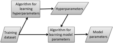
Learning hyperparameters via cross-validation: Hyperparameter is a key parameter in machine learning systems; a good hyperparameter makes it possible to learn a model that has good generalization performance on testing dataset. In practice, hyperparameters are often determined via cross-validation [21]. A popular cross-validation method is called -fold cross-validation. Specifically, we can divide the training dataset into folds. Suppose we are given a hyperparameter. For each fold, we learn the model parameters using the remaining folds as a training dataset and tests the model performance on the fold. Then, we average the performance over the folds. The hyperparameter is determined in a search process such that the average performance in the cross-validation is maximized. Learning hyperparameters is much more computationally expensive than learning model parameters with a given hyperparameter because the former involves many trials of learning model parameters. Figure 1 illustrates the process to learn hyperparameters and model parameters.
Testing performance of the decision function: We often use a testing dataset to measure performance of the learnt model parameters. Suppose the testing dataset consists of , whose labels are , respectively. For regression, the performance is often measured by mean square error (MSE), which is defined as . For classification, the performance is often measured by accuracy (ACC), which is defined as , where is 1 if , otherwise it is 0. A smaller MSE or a higher ACC implies better model parameters.
III-B Problem Definition
Threat model: We assume the attacker knows the training dataset, the ML algorithm, and (optionally) the learnt model parameters. Our threat model is motivated by machine-learning-as-a-service (MLaaS) [6, 1, 18, 25]. MLaaS is an emerging technology to aid users, who have limited computing power and machine learning expertise, to learn an ML model over large datasets. Specifically, a user uploads the training dataset to an MLaaS platform and specifies an ML algorithm. The MLaaS platform uses proprietary algorithms to learn the hyperparameters, then learns the model parameters, and finally certain MLaaS platforms (e.g., BigML [6]) allow the user to download the model parameters to use them locally. Attackers could be such users. We stress that when the model parameters are unknown, our attacks are still applicable as we demonstrate in Section V-B3. Specifically, the attacker can first use model parameter stealing attacks [54] to learn them and then perform our attacks. We note that various MLaaS platforms–such as Amazon Machine Learning and Microsoft Azure Machine Learning–make the ML algorithm public. Moreover, for black-box MLaaS platforms such as Amazon Machine Learning and Microsoft Azure Machine Learning, prior model parameter stealing attacks [54] are applicable.
We define hyperparameter stealing attacks as follows:
Definition 1 (Hyperparameter Stealing Attacks)
Suppose an ML algorithm learns model parameters via minimizing an objective function that is in the form of loss function + regularization term. Given the ML algorithm, the training dataset, and (optionally) the learnt model parameters, hyperparameter stealing attacks aim to estimate the hyperparameter value in the objective function.
Application scenario: One application of our hyperparameter stealing attacks is that a user can use our attacks to learn a model via MLaaS with much less computations (thus much less economical costs), while not sacrificing the model’s testing performance. Specifically, the user can sample a small fraction of the training dataset, learns the model parameters through MLaaS, steals the hyperparameter using our attacks, and re-learns the model parameters via MLaaS using the entire training dataset and the stolen hyperparameter. We will demonstrate this application scenario in Section V-B via simulations and Amazon Machine Learning.
IV Hyperparameter Stealing Attacks
We first introduce our general attack framework. Second, we use several regression and classification algorithms as examples to illustrate how we can use our framework to steal hyperparameters for specific ML algorithms, and we show results of more algorithms in Appendix A.
IV-A Our Attack Framework
Our goal is to steal the hyperparameters in an objective function. For an ML algorithm that uses such hyperparameters, the learnt model parameters are often a minimum of the objective function (see the background knowledge in Section III-A). Therefore, the gradient of the objective function at the learnt model parameters should be , which encodes the relationships between the learnt model parameters and the hyperparameters. We leverage this key observation to steal hyperparameters.
Non-kernel algorithms: We compute the gradient of the objective function at the model parameters and set it to be . Then, we have
| (1) |
where vectors and are defined as follows:
| (10) |
First, Eqn. 1 is a system of linear equations about the hyperparameter . Second, in this system, the number of equations is more than the number of unknown variables (i.e., hyperparameter in our case). Such system is called an overdetermined system in statistics and mathematics. We adopt the linear least square method [30], a popular method to find an approximate solution to an overdetermined system, to solve the hyperparameter in Eqn. 1. More specifically, we estimate the hyperparameter as follows:
| (11) |
Kernel algorithms: Recall that, for kernel algorithms, the model parameters are a linear combination of the kernel mapping of the training instances, i.e., . Therefore, the model parameters can be equivalently represented by the parameters . We replace the variable with in the objective function, compute the gradient of the objective function with respect to , and set the gradient to . Then, we will obtain an overdetermined system. After solving the system with linear least square method, we again estimate the hyperparameter using Eqn. 11 with the vectors and re-defined as follows:
| (20) |
Addressing non-differentiability: Using Eqn. 11 still faces two more challenges: 1) the objective function might not be differentiable at certain dimensions of the model parameters (or ), and 2) the objective function might not be differentiable at certain training instances for the learnt model parameters. For instance, objective functions with regularization are not differentiable at the dimensions where the learnt model parameters are 0, while the objective functions in SVMs might not be differentiable for certain training instances. We address the challenges via constructing the vectors and using the dimensions and training instances at which the objective function is differentiable. Note that using less dimensions of the model parameters is equivalent to using less equations in the overdetermined system shown in Eqn. 1. Once we have at least one dimension of the model parameters and one training instance at which the objective function is differentiable, we can estimate the hyperparameter.
Attack procedure: We summarize our hyperparameter stealing attacks in the following two steps:
-
Step I. The attacker computes the vectors and for a given training dataset, a given ML algorithm, and the learnt model parameters.
-
Step II. The attacker estimates the hyperparameter using Eqn. 11.
More than one hyperparameter: We note that, for conciseness, we focus on ML algorithms whose objective functions have a single hyperparameter in the main text of this paper. However, our attack framework is applicable and can be easily extended to ML algorithms that use more than one hyperparameter. Specifically, we can still estimate the hyperparameters using Eqn. 11 with the vector expanded to be a matrix, where each column corresponds to the gradient of a regularization term with respect to the model parameters. We use an example ML algorithm, i.e., Elastic Net [58], with two hyperparameters to illustrate our attacks in Appendix B.
Next, we use various popular regression and classification algorithms to illustrate our attacks. In particular, we will discuss how we can compute the vectors and . We will focus on linear and kernel ML algorithms for simplicity, and we will show results on neural networks in Appendix C. We note that the ML algorithms we study are widely deployed by MLaaS. For instance, logistic regression is deployed by Amazon Machine Learning, Microsoft Azure Machine Learning, BigML, etc.; SVM is employed by Microsoft Azure Machine Learning, Google Cloud Platform, and PredictionIO.
IV-B Attacks to Regression Algorithms
IV-B1 Linear Regression Algorithms
We demonstrate our attacks to popular linear regression algorithms including Ridge Regression (RR) [19] and LASSO [53]. Both algorithms use least square loss function, and their regularization terms are and , respectively. Due to the limited space, we show attack details for RR, and the details for LASSO are shown in Appendix A. The objective function of RR is . We compute the gradient of the objective function with respect to , and we have . By setting the gradient to be , we can estimate using Eqn. 11 with and .
IV-B2 Kernel Regression Algorithms
We use kernel ridge regression (KRR) [55] as an example to illustrate our attacks. Similar to linear RR, KRR uses least square loss function and regularization. After we represent the model parameters using , the objective function of KRR is , where matrix , whose th entry is . In machine learning, is called gram matrix and is positive definite. By computing the gradient of the objective function with respect to and setting it to be 0, we have . is invertible as it is positive definite. Therefore, we multiply both sides of the above equation with . Then, we can estimate using Eqn. 11 with and . Our attacks are applicable to any kernel function. In our experiments, we will adopt the widely used Gaussian kernel.
IV-C Attacks to Classification Algorithms
IV-C1 Linear Classification Algorithms
We demonstrate our attacks to four popular linear classification algorithms: support vector machine with regular hinge loss function (SVM-RHL), support vector machine with squared hinge loss function (SVM-SHL), -regularized logistic regression (L1-LR), and -regularized logistic regression (L2-LR). These four algorithms enable us to compare different regularization terms and different loss functions. For simplicity, we show attack details for L1-LR, and defer details for other algorithms to Appendix A. L1-LR enables us to illustrate how we address the challenge where the objective function is not differentiable at certain dimensions of the model parameters.
We focus on binary classification, since multi-class classification is often transformed to multiple binary classification problems via the one-vs-all paradigm. However, our attacks are also applicable to multi-class classification algorithms such as multi-class support vector machine [11] and multi-class logistic regression [11] that use hyperparameters in their objective functions. For binary classification, each training instance has a label .
The objective function of L1-LR is , where = is called cross entropy loss function and is defined to be . The gradient of the objective function is , where and the th entry of the vector is defined as follows:
| (21) |
is not differentiable when , so we define the derivative at as 0, which means that we do not use the model parameters that are 0 to estimate the hyperparameter. Via setting the gradient to be 0, we can estimate using Eqn. 11 with and .
IV-C2 Kernel Classification Algorithms
We demonstrate our attacks to the kernel version of the above four linear classification algorithms: kernel support vector machine with regular hinge loss function (KSVM-RHL), kernel support vector machine with squared hinge loss function (KSVM-SHL), -regularized kernel LR (L1-KLR), and -regularized kernel LR (L2-KLR). We show attack details for KSVM-RHL, and defer details for the other algorithms in Appendix A. KSVM-RHL enables us to illustrate how we can address the challenge where the objective function is non-differentiable for certain training instances. Again, we focus on binary classification.
The objective function of KSVM-RHL is , where is called regular hinge loss function. is the th column of the gram matrix . The gradient of the loss function with respect to is:
| (22) |
where is non-differentiable when satisfies . We estimate using that satisfy . Specifically, via setting the gradient of the objective function to be , we estimate using Eqn. 11 with and , where is an indicator function with value 1 if and 0 otherwise.
V Evaluations
V-A Theoretical Evaluations
We aim to evaluate the effectiveness of our hyperparameter stealing attacks theoretically. In particular, we show that 1) when the learnt model parameters are an exact minimum of the objective function, our attacks can obtain the exact hyperparameter value, and 2) when the model parameters deviate from their closest minimum of the objective function with a small difference, then the estimation error of our attacks is a linear function of the small difference. Specifically, our theoretical analysis can be summarized in the following theorems.
Theorem 1
Suppose an ML algorithm learns model parameters via minimizing an objective function which is in the form of loss function + regularization term, is the true hyperparameter value, and the learnt model parameters (or for kernel algorithms) are an exact minimum of the objective function. Then, our attacks can obtain the exact true hyperparameter value, i.e., .
Proof:
See Appendix D. ∎
Theorem 2
Suppose an ML algorithm learns model parameters via minimizing an objective function which is in the form of loss function + regularization term, is the true hyperparameter value, the learnt model parameters are (or for kernel algorithms), and (or ) is the minimum of the objective function that is closest to (or ). We denote and . Then, when or , the difference between the estimated hyperparameter and the true hyperparameter can be bounded as follows:
| Non-kernel algorithms: | |||
| (23) | |||
| Kernel algorithms: | |||
| (24) |
where is the gradient of at and is the gradient of at .
Proof:
See Appendix E. ∎
| Dataset | #Instances | #Features | Type |
|---|---|---|---|
| Diabetes | 442 | 10 | Regression |
| GeoOrig | 1059 | 68 | |
| UJIIndoor | 19937 | 529 | |
| Iris | 100 | 4 | Classification |
| Madelon | 4400 | 500 | |
| Bank | 45210 | 16 |
V-B Empirical Evaluations
V-B1 Experimental Setup
We use several real-world datasets to evaluate the effectiveness of our hyperparameter stealing attacks on the machine learning algorithms we studied. We obtained these datasets from the UCI Machine Learning Repository,111https://archive.ics.uci.edu/ml/datasets.html and their statistics are summarized in Table II. We note that our datasets have significantly different number of instances and features, which represent different application scenarios. We use each dataset as a training dataset.
Implementation: We use the scikit-learn package [40], which implements various machine learning algorithms, to learn model parameters. All experiments are conducted on a laptop with a 2.7GHz CPU and 8GB memory. We predefine a set of hyperparameters which span over a wide range, i.e., , in order to evaluate the effectiveness of our attacks for a wide range of hyperparameters. Note that , so we do not explore negative values for . For each hyperparameter and for each learning algorithm, we learn the corresponding model parameters using the scikit-learn package. For kernel algorithms, we use the Gaussian kernel, where the parameter in the kernel is set to be 10. We implemented our attacks in Python.
Evaluation metric: We evaluate the effectiveness of our attacks using relative estimation error, which is formally defined as follows:
| (25) |
where and are the estimated hyperparameter and true hyperparameter, respectively.
V-B2 Experimental Results for Known Model Parameters
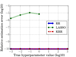
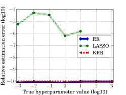
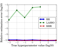
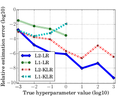
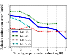
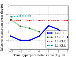
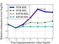
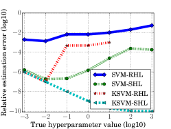
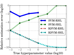
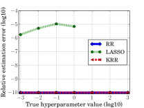
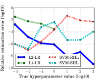
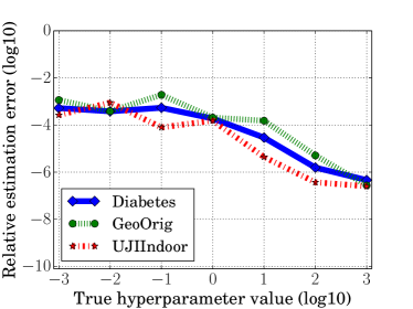
We first show results for the scenario where an attacker knows the training dataset, the learning algorithm, and the model parameters. Figure 2 shows the relative estimation errors for different regression algorithms on the regression datasets. Figure 3 shows the results for logistic regression algorithms on the classification datasets. Figure 4 shows the results for SVM algorithms on the classification datasets. Figure 5 shows the results for three-layer neural networks for regression and classification. In each figure, x-axis represents the true hyperparameter in a particular algorithm, and the y-axis represents the relative estimation error of our attacks at stealing the hyperparameter. For better illustration, we set the relative estimation errors to be when they are smaller than . Note that learning algorithms with regularization require the hyperparameter to be smaller than a maximum value in order to learn meaningful model parameters (please refer to Appendix A for more details). Therefore, in the figures, the data points are missing for such algorithms when the hyperparameter gets larger than , which is different for different training datasets and algorithms. We didn’t show results on kernel LASSO because it is not widely used. Moreover, we didn’t find open-source implementations to learn model parameters in kernel LASSO, and implementing kernel LASSO is out of the scope of this work. However, our attacks are applicable to kernel LASSO.
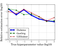
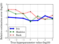
We have two key observations. First, our attacks can accurately estimate the hyperparameter for all learning algorithms we studied and for a wide range of hyperparameter values. Second, we observe that our attacks can more accurately estimate the hyperparameter for Ridge Regression (RR) and Kernel Ridge Regression (KRR) than for other learning algorithms. This is because RR and KRR have analytical solutions for model parameters, and thus the learnt model parameters are the exact minima of the objective functions. In contrast, other learning algorithms we studied do not have analytical solutions for model parameters, and their learnt model parameters are relatively further away from the corresponding minima of the objective functions. Therefore, our attacks have larger estimation errors for these learning algorithms.
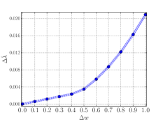
In practice, a learner may use approximate solutions for RR and KRR because computing the exact optimal solutions may be computationally expensive. We evaluate the impact of such approximate solutions on the accuracy of hyperparameter stealing attacks, and compare the results with those predicted by our Theorem 2. Specifically, we use the RR algorithm, adopt the Diabetes dataset, and set the true hyperparameter to be 1. We first compute the optimal model parameters for RR. Then, we modify a model parameter by and estimate the hyperparameter by our attack. Figure 6 shows the estimation error as a function of (we show the absolute estimation error instead of relative estimation error in order to compare the results with Theorem 2). We observe that when is very small, the estimation error is a linear function of . As becomes larger, increases quadratically with . Our observation is consistent with Theorem 2, which shows that the estimation error is linear to the difference between the learnt model parameters and the minimum closest to them when the difference is very small.
V-B3 Experimental Results for Unknown Model Parameters
Our hyperparameter stealing attacks are still applicable when the model parameters are unknown to an attacker, e.g., for black-box MLaaS platforms such as Amazon Machine Learning. Specifically, the attacker can first use the equation-solving-based model parameter stealing attacks proposed in [54] to learn the model parameters and then perform our hyperparameter stealing attacks. Our Theorem 2 bounds the estimation error of hyperparameters with respect to the difference between the stolen model parameters and the closest minimum of the objective function of the ML algorithm.
We also empirically evaluate the effectiveness of our attacks when model parameters are unknown. For instance, Figure 7 shows the relative estimation errors of hyperparameters for regression algorithms and classification algorithms, when the model parameters are unknown but stolen by the model parameter stealing attacks [54]. For simplicity, we only show results on the Diabetes dataset for regression algorithms and on the Iris dataset for classification algorithms, but results on other datasets are similar. Note that LASSO requires the hyperparameter to be smaller than a certain threshold as we discussed in the above, and thus some data points are missing for LASSO. We find that we can still accurately steal the hyperparameters. The reason is that the model parameter stealing attacks can accurately steal the model parameters.
V-B4 Summary
Via empirical evaluations, we have the following observations. First, our attacks can accurately estimate the hyperparameter for all ML algorithms we studied. Second, our attacks can more accurately estimate the hyperparameter for ML algorithms that have analytical solutions of the model parameters. Third, via combining with model parameter stealing attacks, our attacks can accurately estimate the hyperparameter even if the model parameters are unknown.
V-C Implications for MLaaS
We show that a user can use our hyperparamter stealing attacks to learn an accurate model through a machine-learning-as-a-service (MLaaS) platform with much less costs. While different MLaaS platforms have different paradigms, we consider an MLaaS platform (e.g., Amazon Machine Learning [1], Microsoft Azure Machine Learning [25]) that charges a user according to the amount of computation that the MLaaS platform performed to learn the model, and supports two protocols for a user to learn a model. In the first protocol (denoted as Protocol I), the user uploads a training dataset to the MLaaS platform and specifies a learning algorithm; the MLaaS platform learns the hyperparameter using proprietary algorithms and learns the model parameters with the learnt hyperparameter; and then (optionally) the model parameters are sent back to the user. When the model parameters are not sent back to the user, the MLaaS is called black-box. The MLaaS platform (e.g., a black-box platform) does not share the learnt hyperparameter value with the user considering intellectual property and algorithm confidentiality.
In Protocol I, learning the hyperparameter is often the most time-consuming and costly part, because it more or less involves cross-validation. In practice, some users might already have appropriate hyperparameters through domain knowledge. Therefore, the MLaaS platform provides a second protocol (denoted as Protocol II), in which the user uploads a training dataset to the MLaaS platform, defines a hyperparameter value, and specifies a learning algorithm, and then the MLaaS platform produces the model parameters for the given hyperparameter. Protocol II helps users learn models with less economical costs when they already have good hyperparameters. We note that Amazon Machine Learning and Microsoft Azure Machine Learning support the two protocols.
V-C1 Learning an Accurate Model with Less Costs
We demonstrate that a user can use our hyperparameter stealing attacks to learn a model through MLaaS with much less economical costs without sacrificing model performance. In particular, we assume the user does not have a good hyperparameter yet. We compare the following three methods to learn a model through MLaaS. By default, we assume the MLaaS shares the model parameters with the user. If not, the user can use model parameter stealing attacks [54] to steal them.
Method 1 (M1): The user leverages Protocol I supported by the MLaaS platform to learn the model. Specifically, the user uploads the training dataset to the MLaaS platform and specifies a learning algorithm. The MLaaS platform learns the hyperparameter and then learns the model parameters using the learnt hyperparameter. The user then downloads the model parameters.
Method 2 (M2): In order to save economical costs, the user samples of the training dataset uniformly at random and then uses Protocol I to learn a model over the sampled subset of the training dataset. We expect that this method is less computationally expensive than M1, but it may sacrifice performance of the learnt model.
Method 3 (M3): In this method, the user uses our hyperparameter stealing attacks. Specifically, the user first samples of the training dataset uniformly at random. Second, the user learns a model over the sampled training dataset through the MLaaS via Protocol I. We note that, for big data, even a very small fraction (e.g., 1%) of the training dataset could be too large for the user to process locally, so we consider the user uses the MLaaS. Third, the user estimates the hyperparamter learnt by the MLaaS using our hyperparameter stealing attacks. Fourth, the user re-learns a model over the entire training dataset through the MLaaS via Protocol II. We call this strategy “Train-Steal-Retrain”.
V-C2 Comparing the Three Methods Empirically
We first show simulation results of the three methods. For these simulation results, we assume model parameters are known to the user. In the next subsection, we compare the three methods on Amazon Machine Learning, a real-world MLaaS platform.
Setup: For each dataset in Table II, we randomly split it into two halves, which are used as the training dataset and the testing dataset, respectively. We consider the MLaaS learns the hyperparameter through 5-fold cross-validation on the training dataset. We measure the performance of the learnt model through mean square error (MSE) (for regression models) or accuracy (ACC) (for classification models). MSE and ACC are formally defined in Section II. Specifically, we use M1 as a baseline; then we measure the relative MSE (or ACC) error of M2 and M3 over M1. For example, the relative MSE error of M3 is defined as . Moreover, we also measure the speedup of M2 and M3 over M1 with respect to the overall amount of computation required to learn the model. Note that we also include the computation required to steal the hyperparameter for M3.
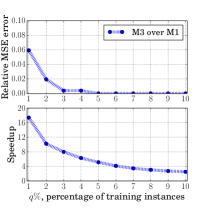
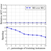
M3 vs. M1: Figure 8 compares M3 with M1 with respect to model performance (measured by relative performance of M3 over M1) and speedup as we sample a larger fraction of training dataset (i.e., gets larger), where the regression algorithm is RR and the classification algorithm is SVM-SHL. Other learning algorithms and datasets have similar results, so we omit them for conciseness.
We observe that M3 can learn a model that is as accurate as the model learnt by M1, while saving a significant amount of computation. Specifically, for RR on the dataset UJIndoorLoc, when we sample 3% of training dataset, M3 learns a model that has almost 0 relative MSE error over M1, but M3 is around 8 times faster than M1. This means that the user can learn an accurate model using M3 with much less economic costs, when the MLaaS platform charges the user according to the amount of computation. For the SVM-SHL algorithm on the Bank dataset, M3 can learn a model that has almost 0 relative ACC error over M1 and is around 15 times faster than M1, when we sample 1% of training dataset. The reason why M3 and M1 can learn models with similar performances is that learning the hyperparameter using a subset of the training dataset changes it slightly and the learning algorithms are relatively robust to small variations of the hyperparameter.
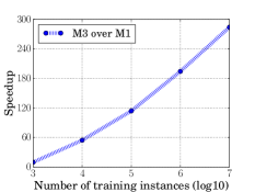
Moreover, we observe that the speedup of M3 over M1 is more significant when the training dataset becomes larger. Figure 9 shows the speedup of M3 over M1 on binary-class training datasets with different sizes, where each class is synthesized via a Gaussian distribution with 10 dimensions. Entries of the mean vectors of the two Gaussian distributions are all 1’s and all -1’s, respectively. Entries of the covariance matrix of the two Gaussian distributions are generated from the standard Gaussian distribution. We select the parameter in M3 such that the relative ACC error is smaller than 0.1%, i.e., M3 learns a model as accurately as M1. The speedup of M3 over M1 is more significant as the training dataset gets larger. This is because the process of learning the hyperparameter has a computational complexity that is higher than linear. M1 learns the hyperparameter over the entire training dataset, while M3 learns it on a sampled subset of training dataset. As a result, the speedup is more significant for larger training datasets. This implies that a user can benefit more by using M3 when the user has a larger training dataset, which is often the case in the era of big data.
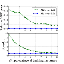
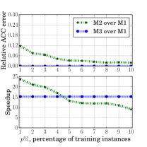
M3 vs. M2: Figure 10 compares M3 with M2 with respect to their relative performance over M1 as we sample more training dataset for M2 (i.e., we increase ). For M3, we set such that the relative MSE (or ACC) error of M3 over M1 is smaller than 0.1%. In particular, and for RR on the UJIndoorLoc dataset and SVM-SHL on the Bank dataset, respectively. We observe that when M3 and M2 achieve the same speedup over M1, the model learnt by M3 is more accurate than that learnt by M2. For instance, for RR on the UJIndoorLoc dataset, M2 has the same speedup as M3 when sampling 10% of training dataset, but M2 has around 4% of relative MSE error while M3’s relative MSE error is almost 0. For SVM-SHL on the Bank dataset, M2 has the same speedup as M3 when sampling 4% to 5% of training dataset, but M2’s relative ACC error is much larger than M3’s.
The reason is that M2 learns both the hyperparameter and the model parameters using a subset of the training dataset. According to Figure 1, the unrepresentativeness of the subset is “doubled” because 1) it directly influences the model parameters, and 2) it influences the hyperparameter, through which it indirectly influences the model parameters. In contrast, in M3, such unrepresentativeness only influences the hyperparameter and the learning algorithms are relatively robust to small variations of the hyperparameter.
V-C3 Attacking Amazon Machine Learning
We also evaluate the three methods using Amazon Machine Learning [1]. Amazon Machine Learning is a black-box MLaaS platform, i.e., it does not disclose model parameters nor hyperparameters to users. However, the ML algorithm is known to users, e.g., the default algorithm is logistic regression. In our experiments, we use Amazon Machine Learning to learn a logistic regression model (with regularization) for the Bank dataset. We leverage the SigOpt API [46], a hyperparameter tuning service for Amazon Machine Learning, to learn the hyperparameter. We obtained a free API token from SigOpt.
We split the Bank dataset into two halves; one for training and the other for testing. For M2 and M3, we sampled 15% and 3% of the training dataset, respectively, i.e., p%=15% and q%=3% (we selected these settings such that M2 and M3 have around the same overall training costs). Since Amazon Machine Learning is black-box, we use the model parameter stealing attack [54] to steal model parameters in our M3. Specifically, in M3, we first used 3% of the training dataset to learn a logistic regression model. Amazon discloses the prediction API of the learnt model. Second, we queried the prediction API for 200 testing examples and used the equation-solving-based attack [54] to steal the model parameters. Third, we used our hyperparameter stealing attack to estimate the hyperparameter. Fourth, we used the entire training dataset and the stolen hyperparameter to re-train a logistic regression model. We also evaluated the accuracy of the three models learnt by the three methods on the testing data via their prediction APIs.
The overall training costs for M1, M2, and M3 (including the cost of querying the prediction API for stealing model parameters) are $1.02, $0.15, and $0.16, respectively. The cost per query of the prediction API is $0.0001. The relative ACC error of M2 over M1 is 5.1%, while the relative ACC error of M3 over M1 is 0.92%. Therefore, compared to M1, M3 saves training costs significantly with little accuracy loss. When M2 and M3 have around the same training costs, M3 is much more accurate than M2.
V-C4 Summary
Through empirical evaluations, we have the following key observations. First, M3 (i.e., the Train-Steal-Retrain strategy) can learn a model that is as accurate as that learnt by M1 with much less computational costs. This implies that, for the considered MLaaS platforms, a user can use our attacks to learn an accurate model while saving a large amount of economic costs. Second, M3 has bigger speedup over M1 when the training dataset is larger. Third, M3 is more accurate than M2 when having the same speedup over M1.
VI Rounding As a Defense
According to our Theorem 2, the estimation error of the hyperparameter is linear to the difference between the learnt model parameters and the minimum of the objective function that is closest to them. This theorem implies that we could defend against our hyperparameter stealing attacks via increasing such difference. Therefore, we propose that the learner rounds the learnt model parameters before sharing them with the end user. For instance, suppose a model parameter is 0.8675342, rounding the model parameter to one decimal and two decimals results in 0.9 and 0.87, respectively. We note that this rounding technique was also used by Fredrikson et al. [14] and Tramèr et al. [54] to obfuscate confidence scores of model predictions to defend against model inversion attacks and model stealing attacks, respectively.
Next, we perform experiments to empirically evaluate the effectiveness of the rounding technique at defending against our hyperparameter stealing attacks.
VI-A Evaluations
VI-A1 Setup
We use the datasets listed in Table II. Specifically, for each dataset, we first randomly split the dataset into a training dataset and a testing dataset with an equal size. Second, for each ML algorithm we considered, we learn a hyperparameter using the training dataset via 5-fold cross-validation, and learn the model parameters via the learnt hyperparameter and the training dataset. Third, we round each model parameter to a certain number of decimals (we explored from 1 decimal to 5 decimals). Fourth, we estimate the hyperparameter using the rounded model parameters.
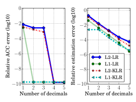
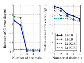
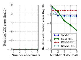
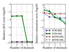
Evaluation metrics: Similar to evaluating the effectiveness of our attacks, the first metric we adopt is the relative estimation error of the hyperparameter value, which is formally defined in Eqn. 25. We say rounding is an effective defense for an ML algorithm if rounding makes the relative estimation error larger. Moreover, we say one ML algorithm can more effectively defend against our attacks than another ML algorithm using rounding, if the relative estimation error of the former algorithm increases more than that of the latter one.
However, relative estimation error alone is insufficient because it only measures security, while ignoring the testing performance of the rounded model parameters. Specifically, severely rounding the model parameters could make the ML algorithm secure against our hyperparameter stealing attacks, but the testing performance of the rounded model parameters might also be affected significantly. Therefore, we also consider a metric to measure the testing-performance loss that is resulted from rounding model parameters. In particular, suppose the unrounded model parameters have a testing MSE (or ACC for classification algorithms), and the rounded model parameters have a testing MSEr (or ACCr) on the same testing dataset. Then, we define the relative MSE error and relative ACC error as and , respectively. Note that the relative MSE error and the relative ACC error used in this section are different from those used in Section V-C. A larger relative estimation error and a smaller relative MSE (or ACC) error indicate a better defense strategy.
VI-A2 Results
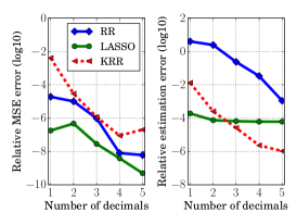
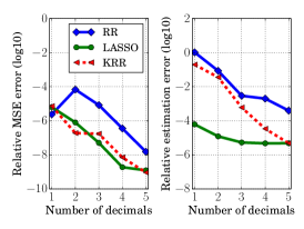
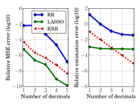
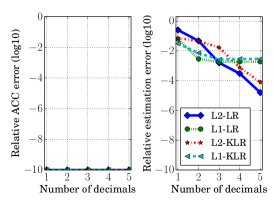
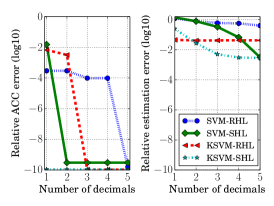
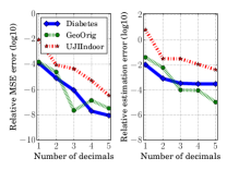
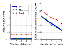
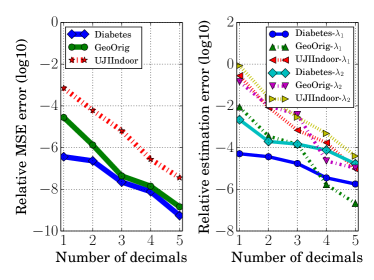
Figure 11, 12, 13, and 14 illustrate defense results for regression, logistic regression, SVM, and three-layer neural networks, respectively. Since we use log scale in the figures, we set the relative MSE (or ACC) errors to be when they are 0.
Rounding is not effective enough for certain ML algorithms: Rounding has small impact on the testing performance of the models. For instance, when we keep one decimal, all ML algorithms have relative MSE (or ACC) errors smaller than 2%. Moreover, rounding model parameters increases the relative estimation errors of our attacks for all ML algorithms. However, for certain ML algorithms, the relative estimation errors are still very small when significantly rounding the model parameters, implying that our attacks are still very effective. For instance, for LASSO, our attacks have relative estimation errors that are consistently smaller than around across the datasets, even if we round the model parameters to one decimal. These results highlight the needs for new countermeasures for certain ML algorithms.
Comparing regularization terms: regularization is more effective than regularization: Different ML algorithms could use different regularization terms, so one natural question is which regularization term can more effectively defend against our attacks using rounding. All the SVM classification algorithms that we studied use regularization term. Therefore, we use results on regression algorithms and logistic regression classification algorithms (i.e., Figure 11 and Figure 12) to compare regularization terms. In particular, we use three pairs: RR vs. LASSO, L2-LR vs. L1-LR, and L2-KLR vs. L1-KLR. The two algorithms in each pair have the same loss function, and use and regularizations, respectively.
We observe that regularization can more effectively defend against our attacks than regularization using rounding. Specifically, the relative estimation errors of RR (or L2-LR or L2-KLR) increases faster than those of LASSO (or L1-LR or L1-KLR), as we round the model parameters to less decimals. For instance, when we round the model parameters to one decimal, the relative estimation errors increase by and for RR and LASSO on the Diabetes dataset, respectively, compared to those without rounding.
These observations are consistent with our Theorem 2. In particular, Appendix F shows our approximations to the gradient in Theorem 2 for RR, LASSO, L2-LR, L2-KLR, L1-LR, and L1-KLR. For an algorithm with regularization, the magnitude of the gradient at the exact model parameters is inversely proportional to the norm of the model parameters. However, if the algorithm has regularization, the magnitude of the gradient is inversely proportional to the norm of the sign of the model parameters. For algorithms with regularization, the learnt model parameters are often small numbers, and thus the norm of the model parameters is smaller than that of the sign of the model parameters. As a result, the magnitude of the gradient for an algorithm with regularization is larger than that for an algorithm with regularization. Therefore, according to Theorem 2, when we round model parameters to less decimals, the estimation errors of an algorithm with regularization increase more than those with regularization.
Comparing loss functions: cross entropy and square hinge loss can more effectively defend against our attacks than regular hinge loss: We also compare defense effectiveness of different loss functions. Since all regression algorithms we studied have the same loss function, we use classification algorithms to compare loss functions. Specifically, we use two triples: (L2-LR, SVM-SHL, SVM-RHL) and (L2-KLR, KSVM-SHL, KSVM-RHL). The three algorithms in each triple use cross entropy loss, square hinge loss, and regular hinge loss, respectively, while all using regularization.
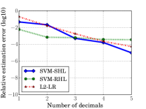
We find that cross entropy and square hinge loss have similar defense effectiveness against our attacks, while they can more effectively defend against our attacks than regular hinge loss using rounding. For instance, Figure 15a compares the relative estimation errors of the triple (L2-LR, SVM-SHL, SVM-RHL) on the dataset Madelon when we use rounding. The relative estimation errors of L2-LR and SVM-SHL increase with a similar speed, but both increase faster than those of SVM-RHL, as we round the model parameters to less decimals. For instance, when we round the model parameters to one decimal, the relative estimation errors increase by , , and for L2-LR, SVM-SHL, SVM-RHL on the dataset Madelon, respectively, compared to those without rounding.
VI-B Implications for MLaaS
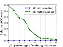
Recall that, in Section V-C, we demonstrate that a user can use M3, i.e., the Train-Steal-Retrain strategy, to learn a model through an MLaaS platform with much less economical costs, while not sacrificing the model’s testing performance. We aim to study whether M3 is still effective if the MLaaS rounds the model parameters. We follow the same experimental setup as in Section V-C, except that the MLaaS platform rounds the model parameters to one decimal before sharing them with the user. Figure 15b compares M3 with M1 with respect to relative ACC error of M3 over M1. Note that the speedups of M3 over M1 are the same with those in Figure 8, so we do not show them again. We observe that M3 can still save many economical costs, though rounding makes the saved costs less. Specifically, when we sample 10% of the training dataset, the relative ACC error of M3 is less than around 0.1% in Figure 15b, while M3 is 6 times faster than M1 (see Figure 8).
VI-C Summary
Through empirical evaluations, we have the following observations. First, rounding model parameters is not effective enough to prevent our attacks for certain ML algorithms. Second, regularization can more effectively defend against our attacks than regularization. Third, cross entropy and square hinge loss have similar defense effectiveness. Moreover, they can more effectively defend against our attacks than regular hinge loss. Fourth, the Train-Steal-Retrain strategy can still save lots of costs when MLaaS adopts rounding.
VII Discussions and Limitations
Assumptions for our Train-Steal-Retrain strategy: A user of an MLaaS platform can benefit from our Train-Steal-Retrain strategy when the following assumptions hold: 1) the hyperparameters can be accurately learnt using a small fraction of the training dataset; 2) the user does not have enough computational resource or ML expertise to learn the hyperparameters locally; and 3) training both the hyperparameters and model parameters using a small fraction of the training dataset does not lead to an accurate model. The validity of the first and third assumptions is data-dependent. We note that Train-Steal-Retrain requires ML expertise, but an attacker can develop it as a service for non-ML-expert users to use.
ML algorithm is unknown: When the ML algorithm is unknown, the problem becomes jointly stealing the ML algorithm and the hyperparameters. Our current attack is defeated in this scenario. In fact, jointly stealing the ML algorithm and the hyperparameters may be impossible in some cases. For instance, logistic regression with a hyperparameter produces a model . On the same training dataset, SVM with a hyperparameter produces a model . If the model parameters and are the same, we cannot distinguish between the logistic regression with hyperparameter and the SVM with a hyperparameter . It is an interesting future work to study jointly stealing ML algorithm and hyperparameters, e.g., show when it is possible and impossible to do so.
Other types of hyperparameters: As a first step towards stealing hyperparameters in machine learning, our work is limited to stealing the hyperparameters that are used to balance between the loss function and the regularization terms in an objective function. Many ML algorithms (please refer to Table I) rely on such hyperparameters. We note that some ML algorithms use other types of hyperparameters. For instance, is a hyperparameter for Nearest Neighbor; the number of trees is a hyperparameter for random forest; and architecture, dropout rate, learning rate, and mini-batch size are important hyperparameters for deep convolutional neural networks. Modern deep convolutional neural networks use dropout [49] instead of conventional / norm to perform regularization. We believe it is an interesting future work to study hyperparameter stealing for these hyperparameters.
Other countermeasures: It is an interesting future work to explore defenses other than rounding model parameters. For instance, like differentially private ML algorithms [12], we could add noise to the objective function.
VIII Conclusion and Future Work
We demonstrate that various ML algorithms are vulnerable to hyperparameter stealing attacks. Our attacks encode the relationships between hyperparameters, model parameters, and training dataset into a system of linear equations, which is derived by setting the gradient of the objective function to be . Via both theoretical and empirical evaluations, we show that our attacks can accurately steal hyperparameters. Moreover, we find that rounding model parameters can increase the estimation errors of our attacks, with negligible impact on the testing performance of the model. However, for certain ML algorithms, our attacks still achieve very small estimation errors, highlighting the needs for new countermeasures. Future work includes studying security of other types of hyperparameters and new countermeasures.
Acknowledgement: We thank the anonymous reviewers for their constructive comments. We also thank SigOpt for sharing a free API token.
References
- [1] AMAZON ML SERVICES. (2017, May). [Online]. Available: https://aws.amazon.com/cn/machine-learning
- [2] M. Barreno, B. Nelson, R. Sears, A. D. Joseph, and J. D. Tygar, “Can machine learning be secure?” in ACM ASIACCS, 2006.
- [3] B. Biggio, I. Corona, D. Maiorca, B. Nelson, N. Šrndić, P. Laskov, G. Giacinto, and F. Roli, “Evasion attacks against machine learning at test time,” in ECML-PKDD. Springer, 2013.
- [4] B. Biggio, L. Didaci, G. Fumera, and F. Roli, “Poisoning attacks to compromise face templates,” in IEEE ICB, 2013.
- [5] B. Biggio, B. Nelson, and P. Laskov, “Poisoning attacks against support vector machines,” in ICML, 2012.
- [6] BigML. (2017, May). [Online]. Available: https://www.bigml.com
- [7] C. M. Bishop, Pattern recognition and Machine Learning. Springer, 2006.
- [8] X. Cao and N. Z. Gong, “Mitigating evasion attacks to deep neural networks via region-based classification,” in ACSAC, 2017.
- [9] N. Carlini, P. Mishra, T. Vaidya, Y. Zhang, M. Sherr, C. Shields, D. Wagner, and W. Zhou, “Hidden voice commands,” in USENIX Security Symposium, 2016.
- [10] N. Carlini and D. Wagner, “Towards evaluating the robustness of neural networks,” in IEEE S & P, 2017.
- [11] C.-C. Chang and C.-J. Lin, “Libsvm: a library for support vector machines,” ACM TIST, 2011.
- [12] K. Chaudhuri, C. Monteleoni, and A. D. Sarwate, “Differentially private empirical risk minimization,” JMLR, pp. 1069–1109, 2011.
- [13] C. Cortes and V. Vapnik, “Support-vector networks,” Machine learning, 1995.
- [14] M. Fredrikson, S. Jha, and T. Ristenpart, “Model inversion attacks that exploit confidence information and basic countermeasures,” in ACM CCS, 2015.
- [15] M. Fredrikson, E. Lantz, S. Jha, S. Lin, D. Page, and T. Ristenpart, “Privacy in pharmacogenetics: An end-to-end case study of personalized warfarin dosing,” in USENIX Security Symposium, 2014.
- [16] I. Goodfellow, Y. Bengio, and A. Courville, Deep learning. MIT Press, 2016.
- [17] I. J. Goodfellow, J. Shlens, and C. Szegedy, “Explaining and harnessing adversarial examples,” arXiv, 2014.
- [18] Google Cloud Platform. (2017, May). [Online]. Available: https://cloud.google.com/prediction
- [19] A. E. Hoerl and R. W. Kennard, “Ridge regression: Biased estimation for nonorthogonal problems,” Technometrics, 1970.
- [20] D. W. Hosmer Jr, S. Lemeshow, and R. X. Sturdivant, Applied logistic regression. John Wiley & Sons, 2013.
- [21] C.-W. Hsu, C.-C. Chang, C.-J. Lin et al., “A practical guide to support vector classification,” Preprint, 2003.
- [22] L. Huang, A. D. Joseph, B. Nelson, B. I. Rubinstein, and J. Tygar, “Adversarial machine learning,” in ACM AISec, 2011.
- [23] L. Ke, B. Li, and Y. Vorobeychik, “Behavioral experiments in email filter evasion,” in AAAI, 2016.
- [24] M. Kloft and P. Laskov, “Online anomaly detection under adversarial impact,” in AISTATS, 2010.
- [25] M. A. M. Learning. (2017, May). [Online]. Available: https://azure.microsoft.com/sevices/machine-learning
- [26] B. Li and Y. Vorobeychik, “Feature cross-substitution in adversarial classification,” in NIPS, 2014.
- [27] B. Li, Y. Wang, A. Singh, and Y. Vorobeychik, “Data poisoning attacks on factorization-based collaborative filtering,” in NIPS, 2016.
- [28] Y. Liu, X. Chen, C. Liu, and D. Song, “Delving into transferable adversarial examples and black-box attacks,” in ICLR, 2017.
- [29] D. Lowd and C. Meek, “Adversarial learning,” in ACM SIGKDD, 2005.
- [30] D. C. Montgomery, E. A. Peck, and G. G. Vining, Introduction to linear regression analysis. John Wiley & Sons, 2015.
- [31] B. Nelson, M. Barreno, F. J. Chi, A. D. Joseph, B. I. P. Rubinstein, U. Saini, C. Sutton, J. D. Tygar, and K. Xia., “Exploiting machine learning to subvert your spam filter,” in LEET, 2008.
- [32] B. Nelson, M. Barreno, F. J. Chi, A. D. Joseph, B. I. P. Rubinstein, U. Saini, C. Sutton, J. D. Tygar, and K. Xia, “Misleading learners: Co-opting your spam filter,” in Machine Learning in Cyber Trust: Security, Privacy, Reliability, 2009.
- [33] B. Nelson, B. I. Rubinstein, L. Huang, A. D. Joseph, S.-h. Lau, S. J. Lee, S. Rao, A. Tran, and J. D. Tygar, “Near-optimal evasion of convex-inducing classifiers.” in AISTATS, 2010.
- [34] J. Newsome, B. Karp, and D. Song, “Polygraph: Automatically generating signatures for polymorphic worms,” in IEEE S & P, 2005.
- [35] J. Newsome, B. Karp, and D. Song, “Paragraph: Thwarting signature learning by training maliciously,” in RAID Workshop. Springer, 2006.
- [36] N. Papernot, P. McDaniel, I. Goodfellow, S. Jha, Z. B. Celik, and A. Swami, “Practical black-box attacks against machine learning,” in AsiaCCS, 2017.
- [37] N. Papernot, P. McDaniel, S. Jha, M. Fredrikson, Z. B. Celik, and A. Swami, “The limitations of deep learning in adversarial settings,” in EuroS&P, 2016.
- [38] N. Papernot, P. McDaniel, A. Sinha, and M. Wellman, “Towards the science of security and privacy in machine learning,” in Arxiv, 2016.
- [39] N. Papernot, P. McDaniel, X. Wu, S. Jha, and A. Swami, “Distillation as a defense to adversarial perturbations against deep neural networks,” in IEEE S & P, 2016.
- [40] F. Pedregosa, G. Varoquaux, A. Gramfort, V. Michel, B. Thirion, O. Grisel, M. Blondel, P. Prettenhofer, R. Weiss, V. Dubourg et al., “Scikit-learn: Machine learning in python,” JMLR, 2011.
- [41] R. Perdisci, D. Dagon, W. Lee, P. Fogla, and M. Sharif, “Misleading worm signature generators using deliberate noise injection,” in IEEE S & P, 2006.
- [42] A. Pyrgelis, C. Troncoso, and E. D. Cristofaro, “Knock knock, who’s there? membership inference on aggregate location data,” in NDSS, 2018.
- [43] B. I. Rubinstein, B. Nelson, L. Huang, A. D. Joseph, S.-h. Lau, S. Rao, N. Taft, and J. Tygar, “Antidote: understanding and defending against poisoning of anomaly detectors,” in ACM IMC, 2009.
- [44] M. Sharif, S. Bhagavatula, L. Bauer, and K. M. Reiter, “Accessorize to a crime: Real and stealthy attacks on state-of-the-art face recognition,” in ACM CCS, 2016.
- [45] R. Shokri, M. Stronati, C. Song, and V. Shmatikov, “Membership inference attacks against machine learning models,” in IEEE S & P, 2017.
- [46] SigOpt. (2017, December). [Online]. Available: https://sigopt.com/
- [47] C. Smutz and A. Stavrou, “Malicious pdf detection using metadata and structural features,” in ACSAC, 2012.
- [48] C. Song, T. Ristenpart, and V. Shmatikov, “Machine learning models that remember too much,” in CCS, 2017.
- [49] N. Srivastava, G. Hinton, A. Krizhevsky, I. Sutskever, and R. Salakhutdinov, “Dropout: A simple way to prevent neural networks from overfitting,” JMLR, 2014.
- [50] N. Srndic and P. Laskov, “Detection of malicious pdf files based on hierarchical document structure,” in NDSS, 2013.
- [51] N. Srndic and P. Laskov, “Practical evasion of a learning-based classifier: A case study,” in IEEE S & P, 2014.
- [52] C. Szegedy, W. Zaremba, I. Sutskever, J. Bruna, D. Erhan, I. Goodfellow, and R. Fergus, “Intriguing properties of neural networks,” arXiv, 2013.
- [53] R. Tibshirani, “Regression shrinkage and selection via the lasso,” JRSSB, 1996.
- [54] F. Tramèr, F. Zhang, A. Juels, M. K. Reiter, and T. Ristenpart, “Stealing machine learning models via prediction apis,” in USENIX Security Symposium, 2016.
- [55] V. Vovk, “Kernel ridge regression,” in Empirical inference. Springer, 2013.
- [56] W. Xu, Y. Qi, and D. Evans, “Automatically evading classifiers: A case study on pdf malware classifiers,” in NDSS, 2016.
- [57] G. Yang, N. Z. Gong, and Y. Cai, “Fake co-visitation injection attacks to recommender systems,” in NDSS, 2017.
- [58] H. Zou and T. Hastie, “Regularization and variable selection via the elastic net,” JRSSB, 2005.
Appendix A Attacks to Other Learning Algorithms
LASSO: The objective function of LASSO is:
| (26) |
whose gradient is:
where is not differentiable when , so we define the derivative at as 0, which means that we do not use the model parameters that are 0 to estimate the hyperparameter. By setting the gradient to be , we can estimate using Eqn. 11 with and .
We note that if , then . In such cases, we cannot estimate the exact hyperparameter. However, in practice, must hold in order to learn meaningful model parameters.
-regularized LR (L2-LR): Its objective function is
| (27) |
where = , which is called cross entropy loss function. is defined to be . The gradient of the objective function with respect to is:
where is a vector. Via setting the gradient to be 0, we can estimate using Eqn. 11 with and .
SVM with regular hinge loss (SVM-RHL): The objective function of SVM-RHL is:
| (28) |
where is called regular hinge loss function. The gradient with respect to is:
where is non-differentiable at the point where . We estimate using only training instances that satisfy . Specifically, we estimate using Eqn. 11 with and , where is an indicator function with value 1 if and 0 otherwise.
SVM with square hinge loss (SVM-SHL): The objective function of SVM-SHL is:
| (29) |
where is called square hinge loss function. The gradient with respect to is:
Therefore, we estimate using Eqn. 11 with and .
-regularized kernel LR (L1-KLR): Its objective function is:
| (30) | ||||
where and . The gradient of the objective function with respect to is:
where and . Via setting the gradient to be 0 and considering that is invertible, we can estimate using Eqn. 11 with and .
-regularized kernel LR (L2-KLR): Its objective function of L1-KLR is:
| (31) | ||||
where is a cross entropy loss function and . The gradient of the objective function with respect to is:
where . Via setting the gradient to be 0 and considering that is invertible, we can estimate using Eqn. 11 with and .
Kernel SVM with square hinge loss (KSVM-SHL): The objective function of KSVM-SHL is:
| (32) | ||||
where . Following the same methodology we used for SVM-SHL, we estimate using Eqn. 11 with and .
Appendix B More than One Hyperparameter
We use a popular regression algorithm called Elastic Net (ENet) [58] as an example to illustrate how we can apply attacks to learning algorithms with more than one hyperparameter. The objective function of ENet is:
| (33) |
where the loss function is least square and regularization term is the combination of regularization and regularization. We compute the gradient as follows:
where . Similar to LASSO, we do not use the model parameters that are 0 to estimate the hyperparameters. Via setting the gradient to and using the linear least square to solve the overdetermined system, we have:
| (34) |
where , , and .
Figure 17 shows the attack and defense results for ENet on the three regression datasets. We observe that our attacks are effective for learning algorithms with more than one hyperparameter, and rounding is also an effective defense.
Appendix C Neural Network (NN)
We evaluate attack and defense on a three-layer neural network (NN) for both regression and classification.
Regression: The objective function of the three-layer NN for regression is defined as
| (35) |
where ; is the logistic function; is the weight matrix of input layer to hidden layer and is the weight vector of hidden layer to output layer; is the number of hidden units; and are the bias terms of the two layers.
To perform our hyperparameter stealing attack, we can leverage the gradient of with respect to either or . For simplicity, we use . Specifically, the gradient of the objective function of is:
By setting the gradient to be , we can estimat using Eqn. 11 with and .
Classification: The objective function of the three-layer NN for binary classification is defined as
| (36) |
where . Similarly with regression, we use to steal the hyperparameter . The gradient of the objective function of is:
Setting the gradient to be , we can estimat via Eqn. 11 with and .
Appendix D Proof of Theorem 5.1
When is an exact minimum of the objective function, we have . Therefore, we have:
Appendix E Proof of Theorem 5.2
We prove the theorem for linear learning algorithms, as it is similar for kernel learning algorithms. We treat our estimated hyperparameter as a function of model parameters. We expand at using Taylor expansion:
Therefore, = =.
Appendix F Approximations of Gradients
We approximate the gradient in Theorem 2 for RR, LASSO, L2-LR, L2-KLR, L1-LR, and L1-KLR. According to the definition of gradient, we have:
where the division and limit are component-wise for .
RR: We approximate the gradient as follows:
where in the third and fourth equations, we use and for sufficiently small , respectively.
LASSO: We approximate the gradient as follows:
where in the third equation, we use .
L2-LR: We approximate the gradient as follows:
where in the third and fourth equations, we use and for sufficiently small , respectively.
L2-KLR: Similar to L2-LR, we approximate the gradient as:
L1-LR: We approximate the gradient as follows:
L1-KLR: Similar to L1-LR, we approximate the gradient as: