Classifying movie genres by analyzing text reviews
Abstract
This paper proposes a method for classifying movie genres by only looking at text reviews. The data used are from Large Movie Review Dataset v1.0 [4] and IMDb. This paper compared a K-nearest neighbors (KNN) model and a multilayer perceptron (MLP) that uses tf-idf as input features. The paper also discusses different evaluation metrics used when doing multi-label classification. For the data used in this research, the KNN model performed the best with an of and a of .
1 Introduction
By only reading a single text review of a movie it can be difficult to say what the genre of that movie is, but by using text mining techniques on thousands of movie reviews is it possible to predict the genre?
This paper explores the possibility of classifying genres of a movie based only on a text review of that movie. This is an interesting problem because to the naked eye it may seem difficult to predict the genre by only looking at a text review. One example of a review can be seen in the following example:
I liked the film. Some of the action scenes were very interesting, tense and well done. I especially liked the opening scene which had a semi truck in it. A very tense action scene that seemed well done. Some of the transitional scenes were filmed in interesting ways such as time lapse photography, unusual colors, or interesting angles. Also the film is funny is several parts. I also liked how the evil guy was portrayed too. I’d give the film an 8 out of 10.111http://www.imdb.com/title/tt0211938/reviews
From the quoted review, one could probably predict the movie falls in the action genre; however, it would be difficult to predict all three of the genres (action, comedy, crime) that International Movie Database (IMDB) lists. With the use of text mining techniques it is feasible to predict multiple genres based on a review.
There are numerous previous works on classifying the sentiment of reviews, e.g., [4] by [4]. There are fewer scientific papers available on specifically classifying movie genres based on reviews; therefore, inspiration for this paper comes from papers describing classification of text for other or general contexts. One of those papers is [2] where [2] describe how to use a multilayer perceptron (MLP) for genre classification.
All data, in the form of reviews and genres, used in this paper originates from IMDb.
2 Theory
In this section all relevant theory and methodology is described. Table 1 lists basic terminology and a short description of their meaning.
| Name | Description |
|---|---|
| Corpus | A structured set of documents. |
| Document | A list of tokens. In this paper a document refers to one review. |
| Term | A word. |
2.1 Preprocessing
Data preprocessing is important when working with text data because it can reduce the number of features and it formats the data into the desired form [1].
2.1.1 Stop words
Removing stop words is a common type of filtering in text mining. Stop words are words that usually contain little or no information by itself and therefore it is better to remove them. Generally words that occur often can be considered stop words such as the, a and it. [1]
2.1.2 Lemmatization
Lemmatization is the process of converting verbs into their infinitive tense form and nouns into their singular form. The reason for doing this is to reduce words into their basic forms and thus simplify the data. For example am, are and is are converted to be. [1]
2.1.3 Tf-idf
A way of representing a large corpus is to calculate the Term Frequency Inverse Document Frequency (tf-idf) of the corpus and then feed the models the tf-idf. As described in [6] by [6] tf-idf is both efficient and simple for matching a query of words with a document in a corpus. Tf-idf is calculated by multiplying the Term Frequency (tf) with the Inverse Document Frequency (idf) , which is formulated as
| (1) |
where is a document in corpus and is a term. is defined as
| (2) |
and is defined as
| (3) |
where is the number of times occurs in and total number of documents in the corpus.
2.2 Models
2.2.1 Multilayer Perceptron
MLP is a class of feedforward neural network built up by a layered acyclic graph. An MLP consists of at least three layers and non-linear activations. The first layer is called input layer, the second layer is called hidden layer and the third layer is called output layer. The three layers are fully connected which means that every node in the hidden layer is connected to every node in the other layers. MLP is trained using backpropagation, where the weights are updated by calculating the gradient descent with respect to an error function. [3]
2.2.2 K-nearest Neighbors
K-nearest Neighbors (KNN) works by evaluating similarities between entities, where stands for how many neighbors are taken into account during the classification. KNN is different from MLP in the sense that it does not require a computationally heavy training step; instead, all of the computation is done at the classification step. There are multiple ways of calculating the similarity, one way is to calculate the Minkowski distance. The Minkowski distance between two points
| (4) |
and
| (5) |
is defined by
| (6) |
where which is equal to the Euclidean distance. [1]
2.3 Evaluation
When evaluating classifiers it is common to use accuracy, precision and recall as well as Hamming loss. Accuracy, precision and recall are defined by the the four terms true positive (), true negative (), false positive () and false negative () which can be seen in table 2.
| Actual true | Actual false | |
|---|---|---|
| Predicted true | ||
| Predicted false |
Accuracy is a measurement of how correct a model’s predictions are and is defined as
| (7) |
.
Precision is a ratio of how often positive predictions actually are positve and is defined as
| (8) |
.
Recall is a measurement of how good the model is to find all true positives and is defined as
| (9) |
. [5]
It has been shown that when calculating precision and recall on multi-label classifiers, it can be advantageous to use micro averaged precision and recall [8]. The formulas for micro averaged precision are expressed as
| (10) |
| (11) |
where is label index and is number of labels.
Hamming loss is different in the sense that it is a loss and it is defined as the fraction of wrong labels to the total number of labels. Hamming loss can be a good measurement when it comes to evaluating multi-label classifiers. the hamming loss is expressed as
| (12) |
where is number of documents, number of labels, is the target value and is predicted value. [7]
3 Data
Data used in this paper comes from two separate sources. The first source was Large Movie Review Dataset v1.0 [4] which is a dataset for binary sentiment analysis of moview reviews. The dataset contains a total of reviews in raw text together with information on whether the review is positive or negative and a URL to the movie on IMDb. The sentiment information was not used in this paper. Out of the , reviews only were used because of limitations on computational power, resulting in a corpus of documents.
The second source of data was the genres for all reviews which were scraped from the IMDb site. A total of 27 different genres were scraped. A list of all genres can be find in Appendix A. A review can have one genre or multiple genres. For example a review can be for a movie that is both Action, Drama and Thriller at the same time while another move only falls into Drama.
4 Method
This section presents all steps needed to reproduce the results presented in this paper.
4.1 Data collection
In this paper the data comes from two sources where the first is a collection of text reviews. Those reviews were downloaded from Large Movie Review Datasets website 222http://ai.stanford.edu/ amaas/data/sentiment. Because only reviews was used in this paper all of them were from the ‘train‘ folder and split evenly between positive reviews and negative reviews.
The genres for the reviews where obtained by iterating through all reviews and doing the following steps:
-
1.
Save the text of the review.
-
2.
Retrieve IMDb URL to the movie from the Large Movie Review Datasets data.
-
3.
Scrape that movie website for all genres and download the genres.
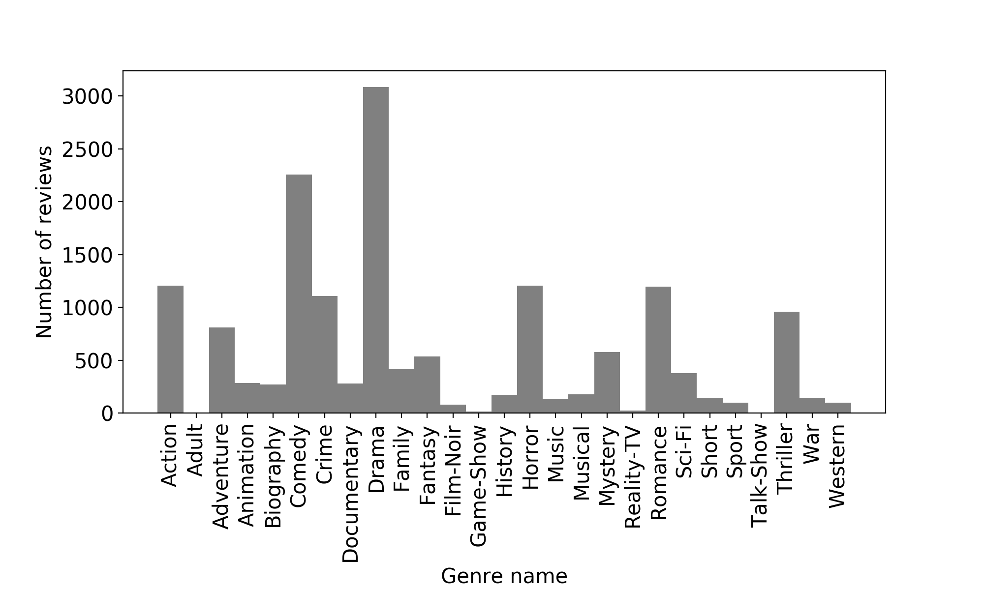
The distribution of genres was plotted in a histogram to check that the scraped data looked reasonable and can be seen in figure 1. All genres with less than reviews corresponding to that genre were removed.

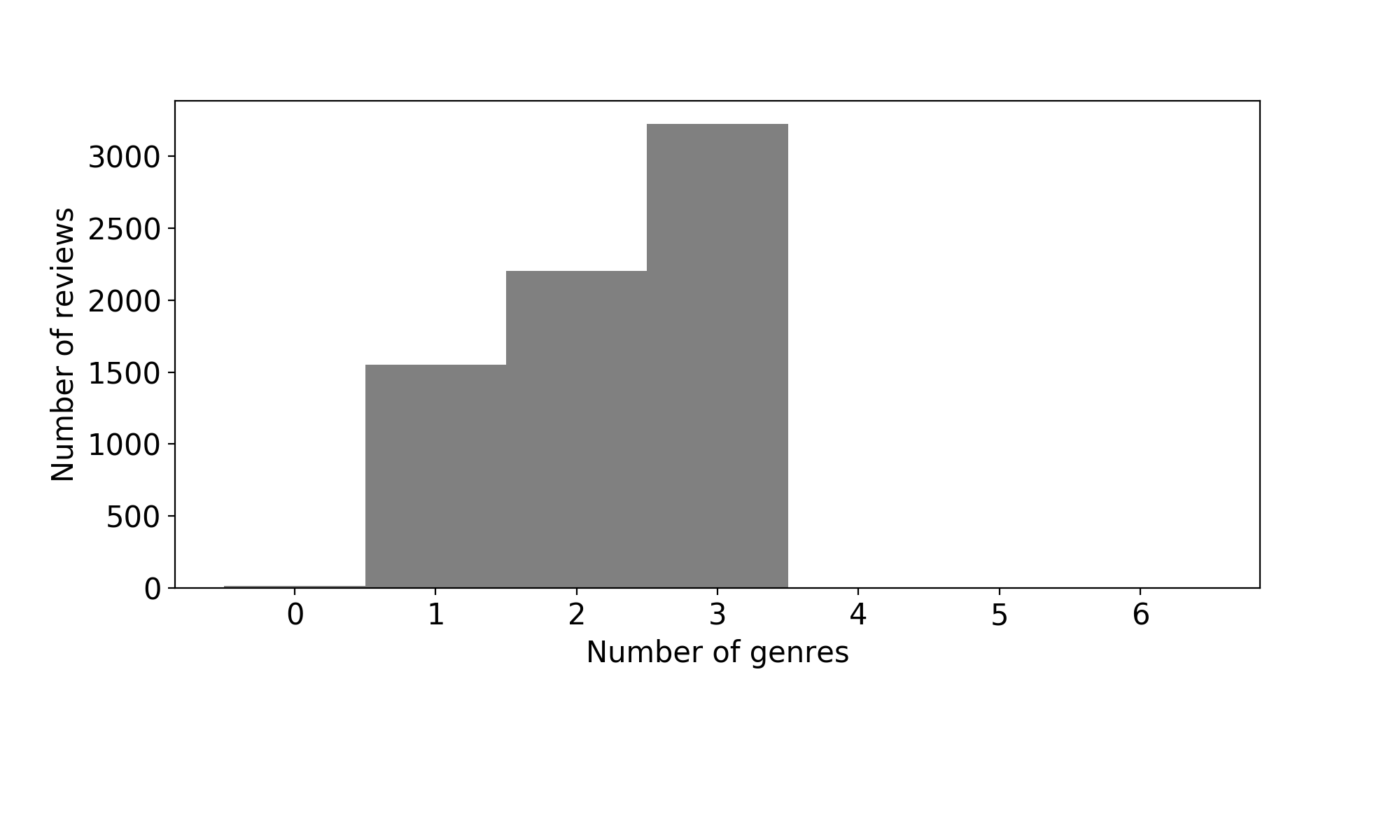
The number of genres per review can be seen in figure 2 and it shows that it is most common for a review to have three different genres; furthermore, it shows that no review has more than three genres.

4.2 Data preprocessing
All reviews were preprocessed according to the following steps:
-
1.
Remove all non-alphanumeric characters.
-
2.
Lower case all tokens.
-
3.
Remove all stopwords.
-
4.
Lemmatize all tokens.
Both the removal of stopwords and lemmatization were done with Python’s33footnotemark: 3 Natural Language Toolkit (NLTK)44footnotemark: 4. Next the reviews and corresponding genres were split into a training set and a test set with devided into the train set and into the test set.
The preprocessed corpus was then used to calculate a tf-idf representing all reviews. The calculation of the tf-idf was done using scikit-learn’s555https://www.python.orgmodule TfidfVectorizer. Both transform and fit were run on the training set and only the transform was run on the test set. The decision to use tf-idf as a data representation is supported by [6] in [6] which concludes that tf-idf is both simple and effective at categorizing relevant words.
4.3 Model
This paper experimented with two different models and compared them against each other. The inspiration for the first model comes from [2] in their paper [2] where they used an MLP for text genre detection. The model used in this paper comes from scikit-learn’s neural_network module and is called MLPClassifier. Table 3 shows all parameters that were changed from the default values.
| Parameter | Value |
| solver | lbfgs |
The second model was a KNN which was chosen because of it is simple and does not require the pre-training that the MLP needs. The implementation of this model comes from scikit-learn’s neighbors module and is called KNeighborsClassifier. The only parameter that was changed after some trial and error was the k-parameter which was set to .
Both models were fitted using the train set and then predictions were done for the test set.
4.4 Evaluation
For evaluation the and was calculated as defined in section 2.3 for both the MLP model and the KNN model. For precision and recall formulas 10 and 13 were used because of their advantage in multi-label classification. The distribution of predicted genres was also shown in a histogram and compared to the target distribution of genres.
Furthermore the ratio of reviews that got zero genres predicted was also calculated and can be expressed as
| (13) |
where is the number of reviews without any predicted genre and is the total amount of predicted reviews.
5 Result
Table 4 shows the , and for the models. The KNN model had a higher accuracy of compared to MPL’s accuracy of and the KNN model had a higher recall but slightly lower precision than the MLP model.
| Model | Accuracy | Precision micro | Recall micro |
|---|---|---|---|
| MLP | |||
| KNN |
Table 5 shows the and for the models, it shows that the KNN model had lower values for both the and compared to the MLP model.
| Model | Hamming loss | No genre ratio |
|---|---|---|
| MLP | ||
| KNN |
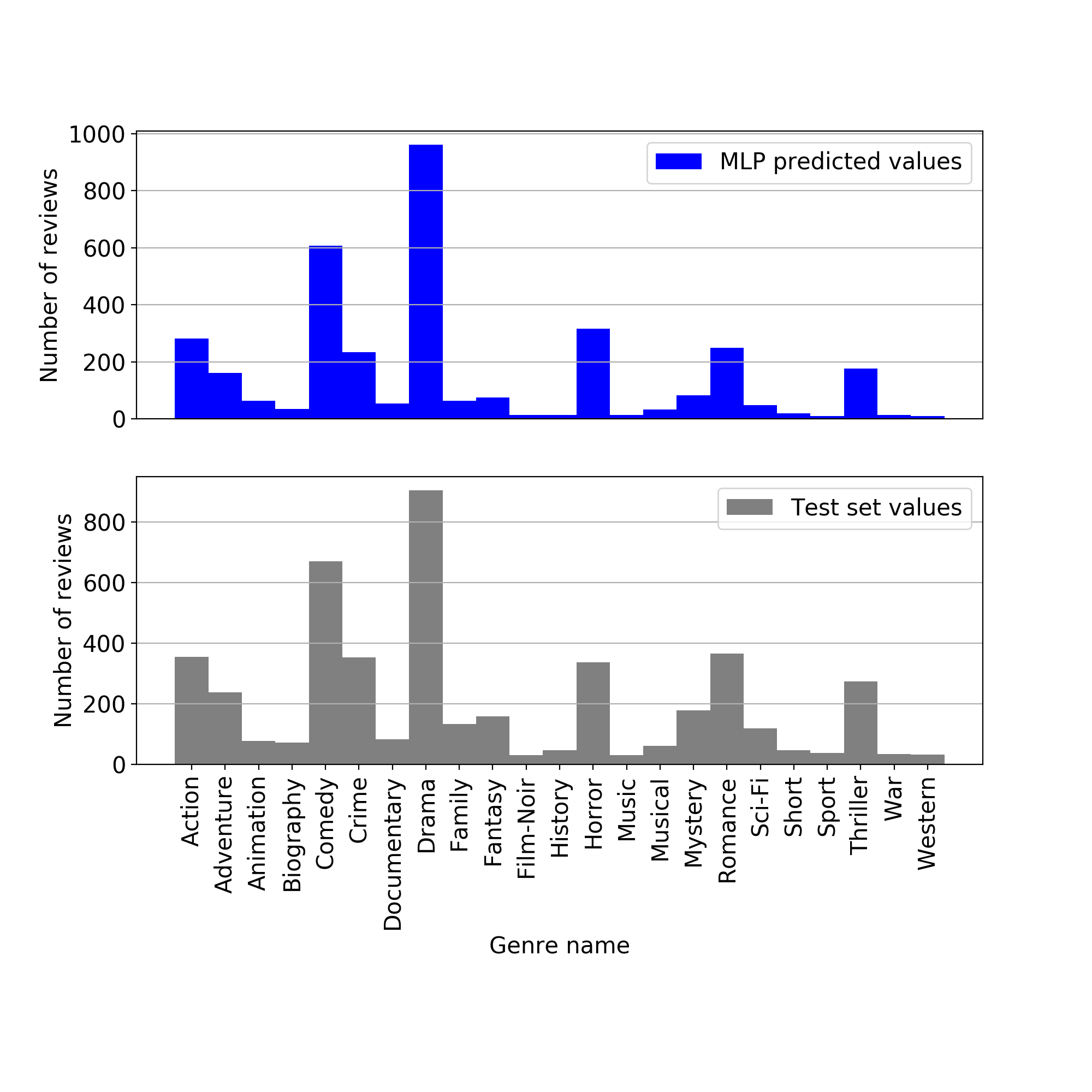
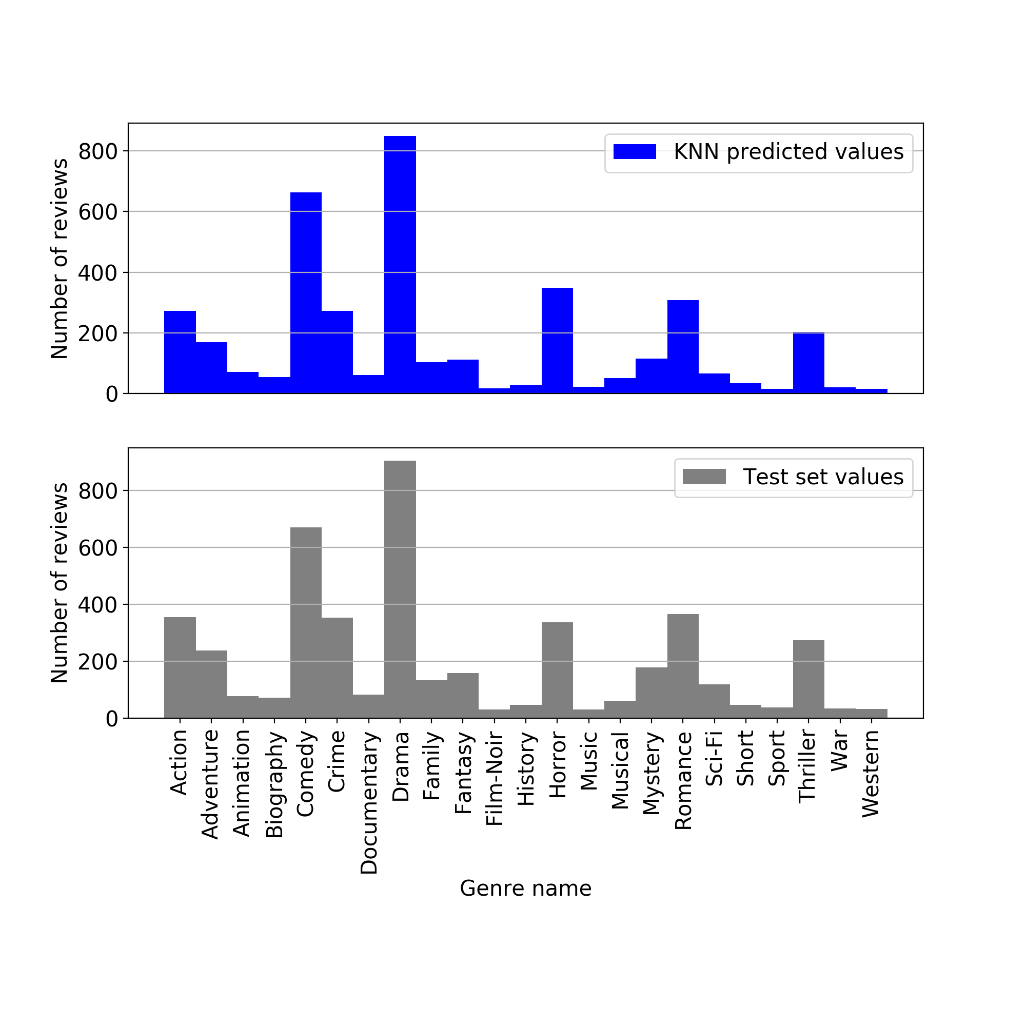
Figure 3 shows the distribution of the genres for the predicted values when using MLP and the test set. The same comparison between KNN and the test set can be seen in figure 4.


6 Discussion
When looking at the results it is apparent that KNN is better than MLP in these experiments. In particular, the stands out between KNN and MLP where KNN got and MLP got which is considered a significant difference. Given that the was relatively high for both models, this result hints that the models only predicted genres when the confidence was high, which resulted in fewer genres being predicted than the target. This can also be confirmed by looking at the figures 3 and 4 where the absolute number of reviews predicted for most genres was lower than the target. This unsatisfyingly low can be explained by the multi-label nature of the problem in this paper. Even if the model correctly predicted 2 out of three genres it is considered a misclassification. A reason for the low accuracy could be that the models appeared to be on the conservative side when predicting genres.
Another factor that affected the performance of the models was the which confirmed that over of the reviews for the KNN model and over of the reviews for the MLP model did not receive any predicted genre. Because no review had zero genres all predictions with zero genres are misclassified and this could be a good place to start when improving the models.
Furthermore, when looking at the it shows that when looking at the individual genres for all reviews the number of wrong predictions are very low which is promising when trying to answer this paper’s main question: whether it is possible to predict the genre of the movie associated with a text review. It should be taken into account that this paper only investigated about movie reviews and the results could change significantly, for better or for worse, if a much larger data set was used. In this paper, some of the genres had very low amounts of training data, which could be why those genres were not predicted in the same frequency as the target. An example of that can be seen by looking at genre Sci-Fi in figure 3.
7 Conclusion
This paper demonstrates that by only looking at text reviews of a movie, there is enough information to predict its genre with an of . This result implies that movie reviews carry latent information about genres. This paper also shows the complexity of doing prediction on multi-label problems, both in implementation and data processing but also when it comes to evaluation. Regular metrics typically work, but they mask the entire picture and the depth of how good a model is.
Finally this paper provides an explanation of the whole process needed to conduct an experiment like this. The process includes downloading a data set, web scraping for extra information, data preprocessing, model tuning and evaluation of the results.
References
- [1] Andreas Hotho, Andreas Nürnberger and Gerhard Paaß “A brief survey of text mining.” In Ldv Forum 20.1, 2005, pp. 19–62
- [2] Brett Kessler, Geoffrey Nunberg and Hinrich Schütze “Automatic Detection of Text Genre” In CoRR cmp-lg/9707002, 1997 URL: http://arxiv.org/abs/cmp-lg/9707002
- [3] Sotiris B Kotsiantis, I Zaharakis and P Pintelas “Supervised machine learning: A review of classification techniques”, 2007
- [4] Andrew L. Maas et al. “Learning Word Vectors for Sentiment Analysis” In Proceedings of the 49th Annual Meeting of the Association for Computational Linguistics: Human Language Technologies Portland, Oregon, USA: Association for Computational Linguistics, 2011, pp. 142–150 URL: http://www.aclweb.org/anthology/P11-1015
- [5] David Martin Powers “Evaluation: from precision, recall and F-measure to ROC, informedness, markedness and correlation” Bioinfo Publications, 2011
- [6] Juan Ramos “Using tf-idf to determine word relevance in document queries” In Proceedings of the first instructional conference on machine learning 242, 2003, pp. 133–142
- [7] Mohammad S Sorower “A literature survey on algorithms for multi-label learning”
- [8] M.. Zhang and Z.. Zhou “A Review on Multi-Label Learning Algorithms” In IEEE Transactions on Knowledge and Data Engineering 26.8, 2014, pp. 1819–1837 DOI: 10.1109/TKDE.2013.39
Appendix A All genres
Action
Adult
Adventure
Animation
Biography
Comedy
Crime
Documentary
Drama
Family
Fantasy
Film-Noir
Game-Show
History
Horror
Music
Musical
Mystery
Reality-TV
Romance
Sci-Fi
Short
Sport
Talk-Show
Thriller
War
Western