500+ Times Faster Than Deep Learning

Abstract.

Deep learning methods are useful for high-dimensional data and are becoming widely used in many areas of software engineering. Deep learners utilizes extensive computational power and can take a long time to train– making it difficult to widely validate and repeat and improve their results. Further, they are not the best solution in all domains. For example, recent results show that for finding related Stack Overflow posts, a tuned SVM performs similarly to a deep learner, but is significantly faster to train.

This paper extends that recent result by clustering the dataset, then tuning very learners within each cluster. This approach is over 500 times faster than deep learning (and over 900 times faster if we use all the cores on a standard laptop computer). Significantly, this faster approach generates classifiers nearly as good (within 2% F1 Score) as the much slower deep learning method. Hence we recommend this faster methods since it is much easier to reproduce and utilizes far fewer CPU resources.

More generally, we recommend that before researchers release research results, that they compare their supposedly sophisticated methods against simpler alternatives (e.g applying simpler learners to build local models).

1. Introduction

Recently, deep learning methods like convolutional neural networks (CNN) have become a popular choice for text mining in SE. Such deep learning works well with high dimensional data (Mou et al., 2016) but are very expensive in terms of time and required CPU.

Type	Abbreviation	Learner Description
G	SVM	Support Vector Machine
G	KNN	K-nearest Neighbors
G	DE_KNN	K-nearest Neighbors tuned using differential evolution (DE)
G	DE_SVM	Support Vector Machines Tuned using differential evolution
G	CNN	Convolution Neural Network
L	KMeans_KNN	Cluster + multiple KNNs
L	KMeans_DE_KNN	Cluster + multiple KNNs tuned via DE
L	KMenas_SVM	Cluster + multiple SVMs
L	KMeans_DE_SVM	Cluster multiple SVMs tuned via DE

Table 1. Combinations of learning algorithms. L= “local models” and G= “global models” which denotes learning from clusters or all of the data (respectively).

In response to the computational problems of deep learners, researchers have tried alternate methods. For example, Fu et al.  (Fu and Menzies, 2017) recently revisited a study by Xu et al.  (Xu et al., 2016) on finding the semantic relatedness of Stack Overflow posts. In that study, a single Stack Overflow question along with its complete answer was called a “knowledge unit” (KU). If any two KUs are semantically related, they are considered as linkable knowledge. Otherwise, they are considered isolated. When Xu et al. applied CNN  (Hubel and Wiesel, 1959) (a specific kind of deep learner), that took 14 hours to train. Fu et al. showed that this computational cost was avoidable by replacing a more complex learner (CNN) with a simpler technique augmented by some hyperparameter optimization. Specifically, Fu et al. shows that support vector machine (SVM) tuned via differential evolution (DE) could perform as well as CNN, while training 84 times faster.

This paper further extends the Fu et al. Using very simple widely used data mining method (KMeans), we can train even faster that Fu et al. and 500 times faster than deep learning (and over 900 times faster if we use all the cores on a standard laptop computer). The core to our approach is (1) building multiple local models then (2) tuning per local model. This paper evaluates this divide and conquer approach by:

1. Exploring the Xu et al. task using SVM and K-nearest-neighbor (KNN) classifiers;

2. Repeating step 1 using hyperparameter tuning– specifically, differential Evolution (DE)– to select control parameters for those learners;

3. Repeats steps 1 and 2 using local modeling; i.e. clustering the data then apply tuning and learning to each cluster;

4. Evaluating these local models in terms of both their training time and performance

Table 1 lists all the learners explored here.

This approach lets us ask and answer the following questions:

• RQ1: Can we reproduce Fu et al.’s results for tuning SVM with differential evolution (DE)?

  Result 1.

  Our DE with SVM perform no worse than Fu et al.

• RQ2: How do the local models compare with global models in both tuned and untuned versions in terms model training time?

  Result 2.

  Local models perform comparably to their global model counterparts, but are 570 times faster in model training time.

  (To be precise, that 570 figure comes from running on a single core. If we distribute the execution cross the eight cores of a standard laptop computer, our training times become 965 times faster.)

• RQ3: How does the performance of local models compare with global models and state-of-the-art deep learner when used with SVM and KNN?

  Result 3.

  Local models performance very nearly as well (within 2% F1 Score) as their global counterpart and the state-of-the-art deep Learner.

Based on these experiments and discoveries, our contribution and outcome from the paper are:

• A dramatically faster solution to the Stack Overflow text mining task first presented by Xu et al. This new method runs three orders of magnitude faster than prior work.

• Support for “not everything needs deep learning”; i.e. sometimes, applying deep learning to a problem may not be the best approach.

• Support for a simplicity-first approach; i.e. simple method like KMeans_DE_SVM can performs as good some of the state of the art models but with a (much) faster training time.

• Support for local modeling. Such local models can significantly reduce training time by clustering data then restricting learning to on each cluster.

• A reproduction package - which can be used to reproduce, improve or refute our results.

The rest of the paper is organized into the following sections Section 2 provides background information that directly relates to our research questions, in addition to laying out the motivation behind our work. In Section 3 a detailed description of our experimental setup and data, along with our performance criteria for evaluation is presented. It is followed by Section 4 the results of the experiments and answers to our research questions are detailed. Section 5 discusses threats to validity. Finally Section 6 concludes the paper with implications and scope for future work.

2. Background

2.1. Motivation

Why obsesses on making software analytics faster? Why not just buy more cloud CPU time? Such a “just throw money at it” approach might not impress researchers like Fisher et al. (Fisher et al., 2012) who define “software analytics” as a work flow that distills large quantities of low-value data down to smaller sets of higher value data. Due to the complexities and computational cost of some kinds of SE analytics, “the luxuries of interactivity, direct manipulation, and fast system response are gone” (Fisher et al., 2012). They characterize modern cloud-based analytics as a throwback to the 1960s-batch processing mainframes where jobs are submitted and then analysts wait, wait, wait for results with “little insight into what’s really going on behind the scenes, how long it will take, or how much it’s going to cost” (Fisher et al., 2012). Fisher et al. document the issues seen by 16 industrial data scientists, one of whom remarks “Fast iteration is key, but incompatible with the say jobs are submitted and processed in the cloud. It’s frustrating to wait for hours, only to realize you need a slight tweak to your feature set.”.

Fisher’s experience matches with our own. We find that the slower the data mining method, the worse the user experience and the fewer the people willing to explore that method. These result is particularly acute in research where data miners have to be run many times to (a) explore the range of possible behaviors resulting from these methods or (b) generate the statistically significant results that can satisfy peer review. To understand the CPU problems with validation, consider the standard validation loop:

    1. FOR L = 20 projects DO
    2.   FOR R = 20 times DO # repeats to satisfy central limit theorem
    3      Randomly divide project.data to B = 10 bins;
    4      FOR i = 1..B DO
    5        test = bin[i]
    6        train = project.data - test
    7.       FOR F = 5 different data filters DO
    8.         train = filter(train) # e.g. over-sample rare classes
    9.         model = leaner(train)
    10.        print report(apply(model,test))
    

Note the problem with this loop- it must call a data miner (at line 9) $L*R*B*F=20,000$ times. While some data miners are very fast (e.g. Naive Bayes), some are not (e.g. deep learning). Worse, several “local learning” results (Menzies et al., [n. d.], 2011; Xia et al., 2008; Menzies et al., 2013) report that software analytics results are specific to the data set being processed- which means that analysts may need to rerun the above loop anytime new data comes to hand.

Note that the above problem is not solvable by (1) waiting for faster CPUs or (2) parallelization. We can no longer rely on Moore’s Law (Moore et al., 1998) to double our computational power very 18 months. Power consumption and heat dissipation issues effectively block further exponential increases to CPU clock frequencies (Moore et al., 1998). As to parallelization, that would require the kinds of environments that Fisher et al. discuss; i.e. environments where it is frustrating to wait for hours, only to realize you need a slight tweak to your feature setting.

Accordingly, in our research, whenever we have a slow and competent result, we explore methods to make that result faster. The rest of this paper offers a case study where local learner significantly speed up than deep learning.

2.2. Deep Learning

Deep learning is a type of machine learning algorithm based on multiple layers of neural networks, where each layer is created with multiple neurons. These layers are interconnected via weights, which are tuned as the model trains. These connections and weights are very specific to models and its performance. According to LeCun et al. (LeCun et al., 2015), deep learning methods are representation-learning methods with multiple levels of representation, obtained by composing simple but non-linear modules that each transforms the representation at one level (starting with the raw input) into a representation at a higher, slightly more abstract level.

Deep learning has been applied to many areas including image processing, natural language processing, genomics etc:

• Wan and Wang (Wan et al., 2014), deep learning tries to resolve the ”Semantic Gap” issue in content based image retrieval process (Smeulders et al., 2000).

• Deep learning has also been used to predict DNA-RNA binding proteins (Alipanahi et al., 2015) which helps to solve problems faced by less sophisticated methods (particularly the problem of the automatic extraction of meaningful features from raw data).

• Deep learning has also recently become established its presence in software engineering effort estimation (Choetkiertikul et al., 2018) and text mining (Choetkiertikul et al., 2016; Mou et al., 2016; White et al., 2016; White et al., 2015; Yuan et al., 2014; Yang et al., 2015).

Deep learning is a computationally expensive method. It often takes hours to weeks to train the models. This makes cross validation and stability of model check very expensive if not impractical. For example, the methods of Xu et al. take 14 hours to terminate or GU et al. (Gu et al., 2016) reported in his paper that his deep learning model took almost 240 hours to train (Gu et al., 2016). Note that if those computations were repeated (say) 20 times for statistically purposes, then those systems would take 11 and 200 days to complete. Worse still, hyperparameter optimization might require 100s to 1000s of repeated runs– which would take another three to 50 years to terminate.

For the above reasons, reproducing deep learning results is a significant problem:

• Most deep learning paper’s baseline methods in SE are either not publicly available or too complex to implement (White et al., 2016; Lam et al., 2015).

• It is not yet common practice for deep learning researchers to share their implementations and data (White et al., 2016; White et al., 2015; Lam et al., 2015; Wang et al., 2016; Choetkiertikul et al., 2016; Gu et al., 2016), where a tiny difference may lead to a huge difference in the results.

• Due to the nature of complexity in implementation and unavailability of original implementation, data or environment it is not possible to implement a deep learner for baseline purpose, and this is one of the reasons for SE community and this paper to directly utilizes the results published for comparison (Lam et al., 2015; Fu and Menzies, 2017).

Hence, much research (including this paper) is forced to compare their new methods with published numbers in deep learning papers (rather than re-running the rig of the other researchers.)

As discussed below, local learning is one method for reducing that runtime.

2.3. Local Learning

When running a data mining algorithm, all the training data can be used to build one training model. Alternatively, the training data can be somehow divided into small pieces and one model learned per piece.

Local models have shown promising results in different studies. Many researchers have found building specialized local models for specific regions of the data provides a better overall performance, thus according to the studies instead of trying to find a generalized model we should try to find best models specific to different region of data. For example, Menzies et al. (Menzies et al., [n. d.]) shows that for defect prediction and effort estimation, lessons learned from models build on small part of data set from PROMISE repository were superior to the generalized model build on all the data. That said, recent studies have suggested for at least for defect prediction, the benefit of local model may be learner specific (Herbold et al., 2017).

This paper explored local learning for a somewhat different perspective. The claim made in this paper is not that local models always performs significantly better. Rather we recommend it since it can lead to significantly faster inference with very little compromise in the performance of the learned model.

More specifically, in this study we observer a three order of magnitude improvement over a prior text mining results by Xu et al (Xu et al., 2016). Hence we recommend local learning since:

• It rarely performs worse than learning from all the data.

• Sometimes it can lead to better performance (Menzies et al., [n. d.], 2011; Bettenburg et al., 2012; Posnett et al., 2011).

• It can lead to significantly faster training times.

The general framework for local learning is shown as a algorithm in Figure 1. This algorithm uses a cluster based model with the training dataset to find diversity in the dataset. This helps to create clusters with similar data. Now different classification models are accessed and improved via hyperparameter tuning on each of the clusters with local data as training dataset. While accessing the model for performance, the test data is sent through the clustering model to predict its probable cluster by calculating similarity measure, next the test data is classified using the local model built on that cluster.

The rest of this paper explores the local learning framework of Figure 1 using the following learning methods:

• K-means for the clustering;

• Differential evolution for the fitting;

• SVM or Kth-nearest neighbor for the classification.

For details on these methods, see later in this paper.

⬇

1 def localLearning (data):

2 models = []

3 predicted = []

4 cluster_model = model₁(args₁) # make clusters

5 cluster_model.fit(data.train)

6 data.train[’cluster’] = cluster_model.labels

7 classification_model = model₂(args₂) # local classifier

8 for i in |cluster|

9 classification_model.fit(data.train[i]) # fitting model

10 models[i] = classification_model

11 #end for

12 data.test[’cluster’]= find nearest cluster for test data

13 for i in |cluster|

14 classification_model = models[i]

15 predicted[i]= classification_model.predict(data.test[i])

16 #end for

17 performance = compare(predicted,data.test[’class’])

18 return performance

Figure 1. Pseudo-code of Local Learning

2.4. Word Embedding

In the case study of this paper, we explore local learning for text mining methods that use word embedding. This is the process of converting words to vectors in order to compare their similarity by comparing cosine similarity between vectors. One method for doing this is a continuous skip-gram model (word2vec), which is a unsupervised two-layer neural network that converts words into semantic vector representations  (Mikolov et al., 2013) and is also used by Fu et al. (Fu and Menzies, 2017) and Xu et al. (Xu et al., 2016) in their paper.

The model learns vector representation of a word (center word) by predicting surrounding words in a context window($c$) by maximizing the mean of log probability of the surrounding words ($w_{i+j}$), given the center word ($w_{i}$) -

(1) $$\frac{1}{n}\sum_{i=1}^{n}\sum_{-c\leq j\leq c,j\neq 0}logp(w_{i+j}|w_{i})$$

The probability $p(w_{i+j}|w_{i})$ is a conditional probability defined by a softmax function -

(2) $$p(w_{i+j}|w_{i})=\frac{exp(v_{w_{i+j}}^{{}^{\prime}T}v_{w_{i}})}{\sum_{w=1}^{|W|}exp(v_{w}^{{}^{\prime}T}v_{w_{i}})}$$

Here the $v_{w}$ and $v_{w}^{{}^{\prime}T}$ are respectively the input and output vectors of a word $w$ in the neural network, and W is the vocabulary of all words in the word corpus. $p(w_{i+j}|w_{i})$ is normalized probability of word $w_{i+j}$ appearing in a specific context for a center word $w_{i}$. To improve the computation efficiency, Mikolove et al.  (Mikolov et al., 2013) proposed hierarchical softmax and negative sampling techniques etc which can also be used for creating word embedding models.

This paper uses the word2vec models trained by Fu et al. (Fu and Menzies, 2017) that converted the Stack Overflow text data into the corresponding vectors. For our experiments, we use $100,000$ randomly selected knowledge units tagged with “java” from Stack Overflow posts table (include titles, questions and answers). This data was pruned by removing superflous HTML tags (while keeping short code snippets in code tag), then fitted into the gensim word2vec module  (Rehurek and Sojka, 2010). This is a python wrapper over original word2vec package where, for word $w_{i}$ in the post is sent to the trained word2vec model to get the corresponding word vector representation $v_{i}$. After converting, all the KUs the output vectors are then used for training and testing the models.

2.5. SVM in Text Mining

Another component of the case study explored here is support vector machines. SVMs are a type of supervised machine learning algorithm which analyzes data using classification or regression analysis. In SVM models the examples are points in space mapped in such a way that separate categories/classes are divided by a clear gap (hyperplane in instance space) (Suykens and Vandewalle, 1999). SVMs execute by transforming the original data space to a higher dimensional space where hyperplane between data from different classes is easier to detect.

SVMs are particularly useful for in text mining can have a very large number of features (Gamon, 2004). In most cases the document vectors are sparse and linearly separable in some hyper-dimensional space (Joachims, 1998).

2.6. KNN in Text Mining

If SVM is our most sophisticated classifier, our simplest is K-Nearest Neighbor (Zhang and Zhou, 2007). KNN is a non-parametric  (Goldberger et al., 2005) method used for classification and regression problems. Here k is the input and refers to the number of closest examples that the model will look for among the training data in the feature space. The output the model gives represents the class to which the test data belongs to and it depends on the majority vote of its k-nearest neighbor  (Mihalcea et al., 2006).

2.7. KMeans Clustering

One way to reduce the computational cost of KNN is, before running a classifier, group data into similar sets of clusters. KMeans is an unsupervised machine learning algorithm that is used for clustering data  (Jain, 2010). In KMeans, k is an input that refers to the number of clusters the data set should be divided into. The algorithm initializes k number of centroids from the data and labels each as a cluster. For each data point it checks which centroid it is closest to, and assigns it to that cluster. After one pass to the data, centroids are recalculated and the process repeats until cluster stability is achieved. This experiments uses the scikit-learn module sklearn.cluster.KMeans (Pedregosa et al., 2011).

⬇

1 def GAP( tData, nrefs=3, cMax = 15): # default settings

2 gaps = []

3 results = create empty dataframe

4 for gap_index, k in enumerate(range(1, cMax)):

5 refDisps = array for inertia

6 for i in range(nrefs):

7 rRef = random(tData) #reference data

8 clf = KMeans(k)

9 clf.fit(rRef)

10 refDisps[i] = model inertia

11 #end for

12 clf = KMeans(k)

13 clf.fit(tData)

14 orgDisp = model inertia with k cluster

15 refDispMean = mean(refDisps)

16 dispDiff = refDispMean - orgDisp

17 gap = log(dispDiff)

18 # append the gap value in the list

19 results = results.append(’clusterCount’: k, ’gap’: gap)

20 gaps[gap_index] = gap

21 return gaps.argmax() # get cluster size with max gap

Figure 2. Pseudo-code of GAP Statistics

SVM	Default Parameter	Tuning Range	Description
C	1.0	[1,50]	Penalty parameter of error term
Kernal	‘rbf’	[‘liner’, ‘poly’, ‘rbf’, ‘sigmoid’]	Specify the kernel type to be used in the algorithms
gamma	1/n_features	[0,1]	Kernel coecient for ‘rbf’, ‘poly’ and ‘sigmoid’
coef0	0	[0,1]	Independent term in kernel function. It is only used in ‘poly’ and ‘sigmoid’
KNN	Default Parameter	Tuning Range	Description
n_neighbors	5	[2,10]	Number of neighbors
weights	‘uniform’	[‘uniform’, ‘distance’]	weight function used for predictions

Table 2. ‘Tuning Range’ of Parameters for SVM and KNN

Picking an appropriate k value for KMeans is a challenge. If k is too small, models will over-fit and fails to capture any larger patterns in the data. On the other hand, if using a large k will increase the variability and hence the level of uncertainty within each cluster. accordingly, this study uses the GAP statistics to determine the optimal number of k or centroids for KMeans  (Mohajer et al., 2011; Tibshirani et al., 2001). The GAP statistic looks at the difference between the dispersion of the clustered data, and the dispersion of a null reference distribution, for increasing k values. It finds the largest k where the gap is bigger than the next gap minus a value that accounts for simulation error. Figure 2 describes the GAP statistic computation (Tibshirani et al., 2001).

2.8. Parameter Tuning with DE

All learners come with “magic parameters” that control their performance. For example, with SVM, there are several parameter that control the SVM kernel. One way to select those parameters is to use hyperparameter optimization via algorithms like Differential Evolution. DE is a stochastic population-based optimization algorithm (Storn and Price, 1997). DE starts with a frontier of randomly generated candidate solutions. For example, when exploring tuning, each member of the frontier would be a different possible set of control settings for (say) an SVM or KNN.

After initializing this frontier, a new candidate solution is generated by extrapolating by some factor $f$ between other items on the frontier. Such extrapolations are performed for all attributes at probability cf. If the candidate is better than one item of the frontier, then the candidate replaces the frontier item. The search then repeats for the remaining frontier items. For the definition of “better“, this study uses the same performance measures as Fu et al.; i.e. “better” means maximizing the objective score of the model based F1 Score.

This process is repeated for lives number of repeated traversals of the frontier. For full details of DE, see fFgure 3. As per Storn’s advice (Storn and Price, 1997) we use

$$f=0.75,\mathit{cf}=0.3,\mathit{lives}=60$$

⬇

1 def DE( n=10, cf=0.3, f=0.7): # default settings

2 frontier = sets of guesses (n=10)

3 best = frontier.1 # any value at all

4 lives = 1

5 while(lives$--$ > 0):

6 tmp = empty

7 for i = 1 to $|$frontier$|$: # size of frontier

8 old = frontier_i

9 x,y,z = any three from frontier, picked at random

10 new= copy(old)

11 for j = 1 to $|$new$|$: # for all attributes

12 if rand() < cf # at probability cf…

13 new.j = $x.j+f*(z.j-y.j)$ # …change item j

14 # end for

15 new = new if better(new,old) else old

16 tmp_i = new

17 if better(new,best) then

18 best = new

19 lives++ # enable one more generation

20 end

21 # end for

22 frontier = tmp

23 # end while

24 return best

Figure 3. Tuner Procedure - as mentioned in Fu et al.'s paper. It is based on Storn's DE optimizer.

For SVM, this study uses the SVM module from Scikit-learn (Pedregosa et al., 2011), a Python package for machine learning, where the following parameters shown in Table 2 are selected for tuning:

• Parameter $C$ is to set the amount of regularization, which controls the trade-off between the errors on training data and the model complexity. A small value for $C$ will generate a simple model with more training errors, while a large value will lead to a complicated model with fewer errors.

• gamma defines how far the influence of a single training example reaches, with low values meaning ’far’ and high values meaning ‘close’.

• coef0 is an independent parameter used in sigmod and polynomial kernel function to scale the data.

Similarly KNN uses different parameters to control how it learns and how it predicts. This study uses KNN module from Scikit-learn, and the parameters in Table 2. For KNN:

• Parameter $n\_neighbors$ is number of neighbors to be used for query to check and classification using a majority vote  (Guo et al., 2003).

• $weight$ is another parameter which is tuned as part of hyperparameter tuning. If set to ‘uniform’, then all the points in each neighborhood are weighted equally. If set to ‘distance’, then the weights are inverse of their distance from the new example (so farther away the point, the less weight it has in deciding the class).

3. Experimental Design

3.1. Data

This experiment uses the same training and testing dataset as Xu et al.  (Xu et al., 2016) and Fu et al.  (Fu and Menzies, 2017). For the reasons discussed in Section 2.2, this study compares our results to those reported by Xu et al.

Our dataset includes 6,400 training examples and 1,600 testing examples. Each class is equally represented in both the training and test datasets, with 1600 of each class in the training dataset and 400 of each class in the test dataset, so no handling of class imbalance is necessary.

Both test and training data are in Pandas dataframe  (McKinney, 2011) format, which includes a post Id, related post id, and a link type which is determined by a score between the 2 posts. The link between 2 posts can be of 4 types depending on the score between the sentences as per Table 3.

Scores	Class ID	Type
1.0	1	duplicate
0.8	2	direct link
0¡x¡0.8	3	indirect link
0.00	4	isolated

Table 3. Classification of data

Figure 4. Model Architecture

For finding word embedding  (Mikolov et al., 2013) of Stack Overflow  (Barua et al., 2014) post data, this paper uses the word2vec model trained by Fu et al. and described in Section 2.4. The final data that passed to our classifiers is similar to Table 4.

ID	Post Id	Related Post Id	Link Type Id	Post Id Vec	Related Post Id Vec	Output
0	283	297	1	[…]	[…]	[…]
1	56	68	2	[…]	[…]	[…]
2	5	16	3	[…]	[…]	[…]
3	9083	6841	4	[…]	[…]	[…]

Table 4. Training/Test data in Pandas.dataframe format.

3.2. Method

Training a models and hyper-parameter tuning technique can take much time, depending on the complexity of the training dataset. This makes it harder to perform cross validation or repeatability of prior results. This study check if dividing up the data into small clusters and then train and tune models within each cluster, reduces the overall learner’s training time. In order to do this the data is clustered first, then a model is built for each cluster. This process is shown Figure 4.

For the clustering algorithm KMeans algorithm from Scikit-learn has been used. For the parameters, this study used the k-means++ algorithm  (Arthur and Vassilvitskii, 2007) for the initialization of cluster centroids. In order to choose k, the number of clusters, the GAP statistic method, discussed in Figure 2 has been utilized.

For each cluster, a learner is built that is tuned specifically for that cluster. This study looks at two different learners, SVM and KNN. As discussed above, to tune the learners, DE is being used, specifically Fu et al.'s DE implementation. The study uses F1 Score  (Sokolova et al., 2006) to evaluate the intermediate models in DE, as F1 Score is calculated as the trade-off between precision and recall. This will help us to get models which have both good precision and recall.

To use the model, the test data is first sent to KMeans to find the cluster which it should belong to by calculating vector distance from all cluster’s centroid and returning the cluster with minimum distance. Then the model predict the class using that cluster's learner.

In this study a 10-fold cross validation  (Kohavi et al., 1995) has been used, which was repeated 10 times for the training data. Thus, the results are the mean of 100 models. Each learner (SVM or KNN) on each cluster has been trained on 90% of the data from that cluster and tuned on rest of the 10% and then tested on the untouched test data set.

3.3. Performance Criteria

For evaluating the described model, this study collects and present the same metrics for performance evaluation as Xu et al. and Fu et al., in order to compare results. These metrics are precision, recall and F1 Score. This multiclass classification problem have 4 classes denoted as Duplicate(C1), Direct Link(C2), Indirect Link(C3) and Isolated(C4). The result presents class-wise metrics as well as the mean for the whole model.

		Classified as
		$C_{1}$	$C_{2}$	$C_{3}$	$C_{4}$
Actual	$C_{1}$	$C_{11}$	$C_{12}$	$C_{13}$	$C_{14}$
	$C_{2}$	$C_{21}$	$C_{22}$	$C_{23}$	$C_{24}$
	$C_{3}$	$C_{31}$	$C_{32}$	$C_{33}$	$C_{34}$
	$C_{4}$	$C_{41}$	$C_{42}$	$C_{43}$	$C_{44}$

Table 5. Confusion Matrix

From the confusion matrix describe in Table 5, it can be observed that the correct predictions are the one with label Cii for a class Ci. And from this we will be able to calculate our evaluation matrix. Using this nomenclature, the evaluation metric F1 Score can be defined as follows:

(3) $$\mathit{precision}=\frac{C_{ii}}{\sum\limits_{i}C_{ij}}$$

(4) $$\mathit{recall}=\frac{C_{ii}}{\sum\limits_{i}C_{ji}}$$

(5) $$\mathit{F1}=\frac{2*\mathit{recall}*\mathit{precision}}{(\mathit{precision}+\mathit{recall})}$$

3.4. Statistical Analysis

In order to compare results of the local models with other models, there are two useful tests: significance tests  (Bentler and Bonett, 1980) and effect size tests  (Rosenthal et al., 1994) (Chen and Popovich, 2002).

• Significance tests assess if results are distinct enough to be considered different;

• Effect size tells us whether that difference is large enough to be interesting.

After Wu et al., this study uses the Scott-Knott test, which ranks treatments using a recursive bi-clustering algorithm. At each level, treatments are split where expected value of the treatments has most changed from before. Results in each rank are considered the same according to both significance and effect size tests. As per the recommendations of Wu et al., the Scott-Knott test uses the nonparametric bootstrap  (Efron, 1982) method and Cliffs’ Delta. Note that these two tests are also used and endorsed by other SE researchers (Ghotra et al., 2015).

Class	F1 Score Mean
	Our DE_SVM Fu’s DE_SVM
Duplicate	92 88
Direct link	91 84
Indirect link	98 97
Isolated	93 91
Overall	93 90

Table 6. Comparison of all performance measure between Our DE_SVM and Fu et al.'s DE_SVM

4. Results

RQ1: Can we reproduce Fu et al.'s results for tuning SVM with differential evolution (DE)?

This study uses same differential evolution with SVM for both global and local models. Thus to compare with Fu’s DE with SVM as global model, the first task as part of this experiment was to recreate Fu et al.'s work so that this study have a baseline to measure against. Hence, this research question is a “sanity check” that must be passed before moving on to the other, more interesting research questions.

The study uses the same SVM from Scikit-learn with the parameters tuned as mentioned in Table 2. Here the training time of the DE+SVM model is also compared with Fu et al.'s model. Table 6 shows the class by class comparison for all the performance measure this study is using.

From Table 6 it can be seen that our results with SVM with DE for hyperparameter tuning  (Duan et al., 2003) (Fu and Menzies, 2017) similar to the results of Fu et al. It can be observed from this figure that for most of the cases apart from class 3, the model has performed a little better, but the delta between the performance is very small.

Hence the answer to our RQ1, is that this study has successfully implemented Fu et al.'s SVM. Hence, we can move to more interesting questions.

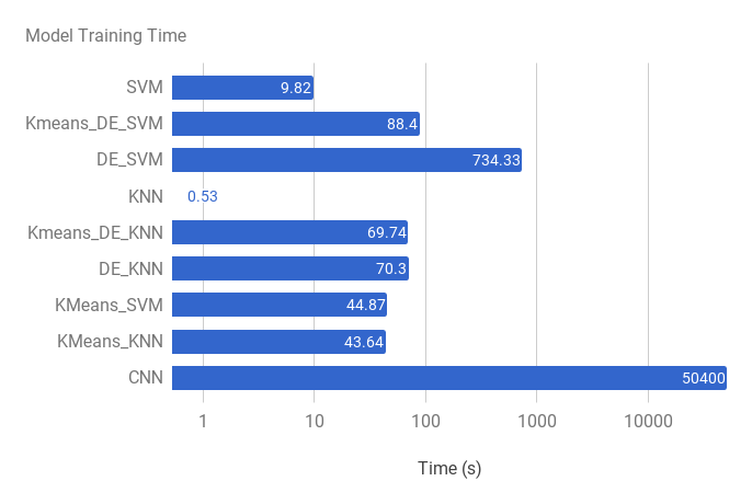
Figure 5. Training time comparison between models in Log Scale. In the above, the Xu et al. 2016 results are labelled “CNN” and the Fu et al. 2017 results are labelled “DE_SVM”.

RQ2: How do the local models compare with global models in both tuned and untuned versions in terms model training time?

For RQ2, this experiment built one model for each clusters using either normal or tuned versions of SVM or KNN (where tuning was performed with DE): For the default SVM and KNN the experiment uses the default parameters, described in Table 1.

As discussed above, this study have used the GAP statistic (Mohajer et al., 2011) (Tibshirani et al., 2001) for finding the best number of clusters, using minimum and maximum number of clusters as 3 and 15, respectively. As part of the experiment we learned that 13 clusters achieves best results (measured as per the GAP statistic).

This study measures the time taken for this model to train which includes time taken by GAP statistic, KMeans training time, and SVM/KNN with DE training time.

Figure 5 compare the model training time in log scale of all models with the results from XU et al.'s CNN approach. Its apparent from the figure 5 that for this domain KNN and SVM has the fastest runtimes. That said, as describe below, we cannot recommend these methods since, as shown below, they achieve poor F1 Scores.

The figure also shows, when we cluster data and then create local models on each cluster it achieves fast training times. For example, in the case of KMeans_DE_SVM, we achieve an eight-fold speed improvement from using DE_SVM. Further, we see a speed improvement of over 570 faster training time from XU's CNN.

RQ3: How does the performance of local models compare with global models and state-of-the-art Deep Learner when used with SVM and KNN?

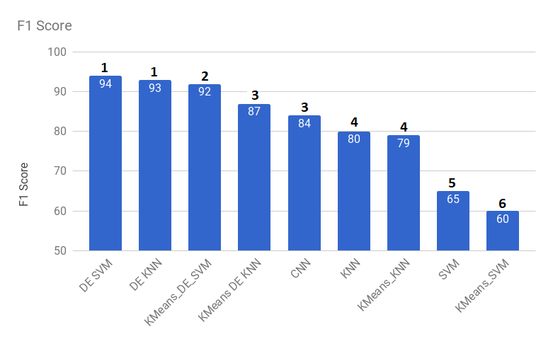
Figure 6. F1 Score comparison for all learners. Numbers above each bar are ranks learned from the Scott-Knot statistical test. Clusters have different ranks if they are determined to be different by both a significance test (bootstrapping) and an effect size test (Cliffs’ Delta). For example, the first two bars have the same rank while the third bar has a different rank. In the above, the Xu et al. 2016 results are labelled “CNN” and the Fu et al. 2017 results are labelled “DE_SVM”.

The final part of our research question was to check if the local models performance is comparable to Fu et al.’s DE_SVM and the XU’s state of the art CNN. To evaluate the performance of the models this study compares F1 performance measures described in Section 3.3. As mentioned in the section, a 10 fold * 10 repeat cross validation was performed, so all the results are mean of 100 models created.

Figure 6 shows our F1 Score results (mean result across all 4 class of Table 6). The numbers on top of each bar show the results of statistical tests. Bars with the same rank are statistically indistinguishable. Note that these results should be discussed with respect to the runtime results shown above:

• In Figure 5, we saw that CNN was our slowest learning method. We would excuse this slowness and endorse its use if the performance scores for this extremely slow method was outstandingly high. This is not the case: as seen Figure 6, CNN is beaten by many of the treatments shown here.

• In Figure 5, DE_SVM was our second slowest method. Again, we would endorse this approach if nothing else comes close to it in terms of performance. While KMeans_DE_SVM is significantly different (as shown by our Scott-Knott results), the median performance delta is very small indeed (median F1 Score scores of 94 vs 92). This is an important pragmatic consideration since, as shown in Figure 5, the learning time of KMeans_DE_SVM was 743/88 = 840% faster than that of DE_SVM

In summary, we recommend one of our local learning method (KMeans_DE_SVM) since:

• It is 840% faster than the prior state-of-the-art results (Fu et al.’s 2017 DE_SVM method);

• On a single core machine, it is 570 times faster than the prior state-of-the-art before that (Xu et al.’s 2016 CNN method);

• On a standard laptop with 8 cores, KMeans_DE_SVM runs 965 times faster than Xu et al.’s CNN method;

• Our local learner performs better than Xu et al. and only a tiny fraction worse than Fu et al. Given these small performance deltas, from a pragmatic engineering perspective, we find it hard to justify the extra computational cost of DE_SVM over KMeans_DE_SVM.

5. THREATS TO VALIDITY

As with any empirical study, biases can affect the final results. Therefore, any conclusions made from this work must be considered with the following issues in mind:

• Sampling bias: threatens any classification experiment; i.e., what matters there may not be true here. For example, the data sets used here is a Stack Overflow dataset and were supplied by one individual. Although this study uses multiple word2vec models to validate with a 10-fold * 10 repeat validations. The text data is of similar format of question pairs.

• Learner bias: For building the model for finding semantic relatedness of question pars in this study, we elected to use Support Vector Machine and K-Nearest Neighbor for classification and KMeans for clustering. This study chose these methods because its results were comparable to the more complicated algorithms and has been successful in text classification field. Classification and clustering is a large and active field and any single study can only use a small subset of the known algorithms.

• Evaluation bias: This paper uses precision, recall and F1 Score as performance measures. Other methods like Concordant - Discordant ratio (Goodman and Kruskal, 1972), Gini Coefficient (Neslin et al., 2006), Kolmogorov Smirnov chart (Guo et al., 2011) that are used for this purpose can also be used for performance evolution in future studies.

• Input bias: For the localization algorithm, this study randomly selects input values for a range to determine the number of clusters, also for hyperparameter tuning using DE, a subset of parameters has been selected for tuning and their range is either the whole range that the parameter accepts or a range that is selected for the study.

6. CONCLUSION

This paper investigates the value of local learning from the perspective of reducing the training time compared to methods for predicting knowledge unit’s relatedness on Stack Overflow. This study clustered the data first; then build local models on each cluster separately; then use the clustering algorithms with the local classification algorithm together to predict. As shown above:

• Clustering the data first and then building local models on those subsets of data shows significant reduction in runtime.

• Using KMeans on the Word Embedding model first to cluster the data into smaller subsets and then running SVM and KNN with their DE versions showed runtime reduction as large as 570 times for KMeans_DE_SVM version with CNN and almost 8 times improvement than its global DE_SVM version with sequential run. And with parallel run the performance improvement for KMeans_DE_SVM version with CNN is 965x and almost 14 times with its global counter part.

• The performance in term of precision, recall and F-score is almost similar to its global counter part and sometime better then the XU’s CNN model.

For future work, we suggest trying several variations of this experiment -

• This study tunes the local models separately, tuning all the local models along with the clustering algorithm together might produce some interesting results.

• Trying to find correlation between number of cluster and training time and performance might give us effect of number of clusters on the prediction model.

References

- (1)
- Alipanahi et al. (2015) Babak Alipanahi, Andrew Delong, Matthew T Weirauch, and Brendan J Frey. 2015. Predicting the sequence specificities of DNA-and RNA-binding proteins by deep learning. Nature biotechnology 33, 8 (2015), 831–838.
- Arthur and Vassilvitskii (2007) David Arthur and Sergei Vassilvitskii. 2007. k-means++: The advantages of careful seeding. In Proceedings of the eighteenth annual ACM-SIAM symposium on Discrete algorithms. Society for Industrial and Applied Mathematics, 1027–1035.
- Barua et al. (2014) Anton Barua, Stephen W Thomas, and Ahmed E Hassan. 2014. What are developers talking about? an analysis of topics and trends in stack overflow. Empirical Software Engineering 19, 3 (2014), 619–654.
- Bentler and Bonett (1980) Peter M Bentler and Douglas G Bonett. 1980. Significance tests and goodness of fit in the analysis of covariance structures. Psychological bulletin 88, 3 (1980), 588.
- Bettenburg et al. (2012) Nicolas Bettenburg, Meiyappan Nagappan, and Ahmed E Hassan. 2012. Think locally, act globally: Improving defect and effort prediction models. In Mining Software Repositories (MSR), 2012 9th IEEE Working Conference on. IEEE, 60–69.
- Chen and Popovich (2002) Peter Y Chen and Paula M Popovich. 2002. Correlation: Parametric and nonparametric measures. Number 137-139. Sage.
- Choetkiertikul et al. (2016) Morakot Choetkiertikul, Hoa Khanh Dam, Truyen Tran, Trang Pham, Aditya Ghose, and Tim Menzies. 2016. A deep learning model for estimating story points. arXiv preprint arXiv:1609.00489 (2016).
- Choetkiertikul et al. (2018) M. Choetkiertikul, H. K. Dam, T. Tran, T. T. M. Pham, A. Ghose, and T. Menzies. 2018. A deep learning model for estimating story points. IEEE Transactions on Software Engineering PP, 99 (2018), 1–1. https://doi.org/10.1109/TSE.2018.2792473
- Duan et al. (2003) Kaibo Duan, S Sathiya Keerthi, and Aun Neow Poo. 2003. Evaluation of simple performance measures for tuning SVM hyperparameters. Neurocomputing 51 (2003), 41–59.
- Efron (1982) Bradley Efron. 1982. The jackknife, the bootstrap and other resampling plans. SIAM.
- Fisher et al. (2012) Danyel Fisher, Rob DeLine, Mary Czerwinski, and Steven Drucker. 2012. Interactions with big data analytics. interactions 19, 3 (2012), 50–59.
- Fu and Menzies (2017) Wei Fu and Tim Menzies. 2017. Easy over Hard: A Case Study on Deep Learning. arXiv preprint arXiv:1703.00133 (2017).
- Gamon (2004) Michael Gamon. 2004. Sentiment classification on customer feedback data: noisy data, large feature vectors, and the role of linguistic analysis. In Proceedings of the 20th international conference on Computational Linguistics. Association for Computational Linguistics, 841.
- Ghotra et al. (2015) Baljinder Ghotra, Shane McIntosh, and Ahmed E Hassan. 2015. Revisiting the impact of classification techniques on the performance of defect prediction models. In Proceedings of the 37th International Conference on Software Engineering-Volume 1. IEEE Press, 789–800.
- Goldberger et al. (2005) Jacob Goldberger, Geoffrey E Hinton, Sam T Roweis, and Ruslan R Salakhutdinov. 2005. Neighbourhood components analysis. In Advances in neural information processing systems. 513–520.
- Goodman and Kruskal (1972) Leo A Goodman and William H Kruskal. 1972. Measures of association for cross classifications, IV: Simplification of asymptotic variances. J. Amer. Statist. Assoc. 67, 338 (1972), 415–421.
- Gu et al. (2016) Xiaodong Gu, Hongyu Zhang, Dongmei Zhang, and Sunghun Kim. 2016. Deep API learning. In Proceedings of the 2016 24th ACM SIGSOFT International Symposium on Foundations of Software Engineering. ACM, 631–642.
- Guo et al. (2003) Gongde Guo, Hui Wang, David Bell, Yaxin Bi, and Kieran Greer. 2003. KNN model-based approach in classification. In CoopIS/DOA/ODBASE, Vol. 2003. Springer, 986–996.
- Guo et al. (2011) Zhen-hai Guo, Jie Wu, Hai-yan Lu, and Jian-zhou Wang. 2011. A case study on a hybrid wind speed forecasting method using BP neural network. Knowledge-based systems 24, 7 (2011), 1048–1056.
- Herbold et al. (2017) Steffen Herbold, Alexander Trautsch, and Jens Grabowski. 2017. Global vs. local models for cross-project defect prediction. Empirical Software Engineering 22, 4 (2017), 1866–1902.
- Hubel and Wiesel (1959) David H Hubel and Torsten N Wiesel. 1959. Receptive fields of single neurones in the cat’s striate cortex. The Journal of physiology 148, 3 (1959), 574–591.
- Jain (2010) Anil K Jain. 2010. Data clustering: 50 years beyond K-means. Pattern recognition letters 31, 8 (2010), 651–666.
- Joachims (1998) Thorsten Joachims. 1998. Text categorization with support vector machines: Learning with many relevant features. Machine learning: ECML-98 (1998), 137–142.
- Kohavi et al. (1995) Ron Kohavi et al. 1995. A study of cross-validation and bootstrap for accuracy estimation and model selection. In Ijcai, Vol. 14. Stanford, CA, 1137–1145.
- Lam et al. (2015) An Ngoc Lam, Anh Tuan Nguyen, Hoan Anh Nguyen, and Tien N Nguyen. 2015. Combining deep learning with information retrieval to localize buggy files for bug reports (n). In Proceedings of the 2015 30th IEEE/ACM International Conference on Automated Software Engineering. IEEE, 476–481.
- LeCun et al. (2015) Yann LeCun, Yoshua Bengio, and Geoffrey Hinton. 2015. Deep learning. Nature 521, 7553 (2015), 436–444.
- McKinney (2011) Wes McKinney. 2011. pandas: a foundational Python library for data analysis and statistics. Python for High Performance and Scientific Computing (2011), 1–9.
- Menzies et al. ([n. d.]) Tim Menzies, Andrew Butcher, David Cok, Andrian Marcus, Lucas Layman, Forrest Shull, Burak Turhan, and Thomas Zimmermann. [n. d.]. Local vs. Global Lessons for Defect Prediction and Effort Estimation,” IEEE Trans. Software Eng., preprint, published online Dec. 2012; http://goo. gl/k6qno. TIM MENZIES is a full professor in computer science at the Lane. In Department of Computer Science and Electrical Engineering, West Virginia University. Contact. Citeseer.
- Menzies et al. (2013) Tim Menzies, Andrew Butcher, David Cok, Andrian Marcus, Lucas Layman, Forrest Shull, Burak Turhan, and Thomas Zimmermann. 2013. Local versus global lessons for defect prediction and effort estimation. IEEE Transactions on software engineering 39, 6 (2013), 822–834.
- Menzies et al. (2011) Tim Menzies, Andrew Butcher, Andrian Marcus, Thomas Zimmermann, and David Cok. 2011. Local vs. global models for effort estimation and defect prediction. In Automated Software Engineering (ASE), 2011 26th IEEE/ACM International Conference on. IEEE, 343–351.
- Mihalcea et al. (2006) Rada Mihalcea, Courtney Corley, Carlo Strapparava, et al. 2006. Corpus-based and knowledge-based measures of text semantic similarity. In AAAI, Vol. 6. 775–780.
- Mikolov et al. (2013) Tomas Mikolov, Ilya Sutskever, Kai Chen, Greg S Corrado, and Jeff Dean. 2013. Distributed representations of words and phrases and their compositionality. In Advances in neural information processing systems. 3111–3119.
- Mohajer et al. (2011) Mojgan Mohajer, Karl-Hans Englmeier, and Volker J Schmid. 2011. A comparison of Gap statistic definitions with and without logarithm function. arXiv preprint arXiv:1103.4767 (2011).
- Moore et al. (1998) Gordon E Moore et al. 1998. Cramming more components onto integrated circuits. Proc. IEEE 86, 1 (1998), 82–85.
- Mou et al. (2016) Lili Mou, Ge Li, Lu Zhang, Tao Wang, and Zhi Jin. 2016. Convolutional Neural Networks over Tree Structures for Programming Language Processing.. In AAAI. 1287–1293.
- Neslin et al. (2006) Scott A Neslin, Sunil Gupta, Wagner Kamakura, Junxiang Lu, and Charlotte H Mason. 2006. Defection detection: Measuring and understanding the predictive accuracy of customer churn models. Journal of marketing research 43, 2 (2006), 204–211.
- Pedregosa et al. (2011) Fabian Pedregosa, Gaël Varoquaux, Alexandre Gramfort, Vincent Michel, Bertrand Thirion, Olivier Grisel, Mathieu Blondel, Peter Prettenhofer, Ron Weiss, Vincent Dubourg, et al. 2011. Scikit-learn: Machine learning in Python. Journal of Machine Learning Research 12, Oct (2011), 2825–2830.
- Posnett et al. (2011) Daryl Posnett, Vladimir Filkov, and Premkumar Devanbu. 2011. Ecological inference in empirical software engineering. In Proceedings of the 2011 26th IEEE/ACM International Conference on Automated Software Engineering. IEEE Computer Society, 362–371.
- Rehurek and Sojka (2010) Radim Rehurek and Petr Sojka. 2010. Software framework for topic modelling with large corpora. In In Proceedings of the LREC 2010 Workshop on New Challenges for NLP Frameworks. Citeseer.
- Rosenthal et al. (1994) Robert Rosenthal, H Cooper, and LV Hedges. 1994. Parametric measures of effect size. The handbook of research synthesis (1994), 231–244.
- Smeulders et al. (2000) Arnold WM Smeulders, Marcel Worring, Simone Santini, Amarnath Gupta, and Ramesh Jain. 2000. Content-based image retrieval at the end of the early years. IEEE Transactions on pattern analysis and machine intelligence 22, 12 (2000), 1349–1380.
- Sokolova et al. (2006) Marina Sokolova, Nathalie Japkowicz, and Stan Szpakowicz. 2006. Beyond accuracy, F-score and ROC: a family of discriminant measures for performance evaluation. In Australian conference on artificial intelligence, Vol. 4304. 1015–1021.
- Storn and Price (1997) Rainer Storn and Kenneth Price. 1997. Differential evolution–a simple and efficient heuristic for global optimization over continuous spaces. Journal of global optimization 11, 4 (1997), 341–359.
- Suykens and Vandewalle (1999) Johan AK Suykens and Joos Vandewalle. 1999. Least squares support vector machine classifiers. Neural processing letters 9, 3 (1999), 293–300.
- Tibshirani et al. (2001) Robert Tibshirani, Guenther Walther, and Trevor Hastie. 2001. Estimating the number of clusters in a data set via the gap statistic. Journal of the Royal Statistical Society: Series B (Statistical Methodology) 63, 2 (2001), 411–423.
- Wan et al. (2014) Ji Wan, Dayong Wang, Steven Chu Hong Hoi, Pengcheng Wu, Jianke Zhu, Yongdong Zhang, and Jintao Li. 2014. Deep learning for content-based image retrieval: A comprehensive study. In Proceedings of the 22nd ACM international conference on Multimedia. ACM, 157–166.
- Wang et al. (2016) Song Wang, Taiyue Liu, and Lin Tan. 2016. Automatically learning semantic features for defect prediction. In Proceedings of the 38th International Conference on Software Engineering. ACM, 297–308.
- Wang et al. (2013) Tiantian Wang, Mark Harman, Yue Jia, and Jens Krinke. 2013. Searching for Better Configurations: A Rigorous Approach to Clone Evaluation. In Proceedings of the 2013 9th Joint Meeting on Foundations of Software Engineering (ESEC/FSE 2013). ACM, New York, NY, USA, 455–465. https://doi.org/10.1145/2491411.2491420
- White et al. (2016) Martin White, Michele Tufano, Christopher Vendome, and Denys Poshyvanyk. 2016. Deep learning code fragments for code clone detection. In Proceedings of the 31st IEEE/ACM International Conference on Automated Software Engineering. ACM, 87–98.
- White et al. (2015) Martin White, Christopher Vendome, Mario Linares-Vásquez, and Denys Poshyvanyk. 2015. Toward deep learning software repositories. In Mining Software Repositories (MSR), 2015 IEEE/ACM 12th Working Conference on. IEEE, 334–345.
- Xia et al. (2008) Ding-yin Xia, Fei Wu, Xu-qing Zhang, and Yue-ting Zhuang. 2008. Local and global approaches of affinity propagation clustering for large scale data. Journal of Zhejiang University-Science A 9, 10 (2008), 1373–1381.
- Xu et al. (2016) Bowen Xu, Deheng Ye, Zhenchang Xing, Xin Xia, Guibin Chen, and Shanping Li. 2016. Predicting semantically linkable knowledge in developer online forums via convolutional neural network. In Proceedings of the 31st IEEE/ACM International Conference on Automated Software Engineering. ACM, 51–62.
- Yang et al. (2015) Xinli Yang, David Lo, Xin Xia, Yun Zhang, and Jianling Sun. 2015. Deep learning for just-in-time defect prediction. In Software Quality, Reliability and Security (QRS), 2015 IEEE International Conference on. IEEE, 17–26.
- Yuan et al. (2014) Zhenlong Yuan, Yongqiang Lu, Zhaoguo Wang, and Yibo Xue. 2014. Droid-Sec: deep learning in android malware detection. In ACM SIGCOMM Computer Communication Review, Vol. 44. ACM, 371–372.
- Zhang and Zhou (2007) Min-Ling Zhang and Zhi-Hua Zhou. 2007. ML-KNN: A lazy learning approach to multi-label learning. Pattern recognition 40, 7 (2007), 2038–2048.