Loss-based approach to two-piece location-scale distributions with applications to dependent data

Abstract

Two-piece location-scale models are used for modeling data presenting departures from symmetry. In this paper, we propose an objective Bayesian methodology for the tail parameter of two particular distributions of the above family: the skewed exponential power distribution and the skewed generalised logistic distribution. We apply the proposed objective approach to time series models and linear regression models where the error terms follow the distributions object of study. The performance of the proposed approach is illustrated through simulation experiments and real data analysis. The methodology yields improvements in density forecasts, as shown by the analysis we carry out on the electricity prices in Nordpool markets.

Keywords: Bayesian inference, loss-Based prior, objective Bayes,, electricity prices.

MSC: 62F15, 62M10.

1 Introduction

Two-piece location-scale models have been mainly used for modeling data exhibiting departures from symmetry. Moreover, some specific two-piece location-scale distributions have been employed in finance to represent the errors in GARCH-type models, see Zhu and Zinde-Walsh, (2009), Zhu and Galbraith, (2011). Different mechanisms have been presented to obtain skewed distributions by modifying symmetric distributions (Azzalini,, 1985; Fernandez and Steel,, 1998; Mudholkar and Hutson,, 2000). Recently, the objective Bayesian literature focused on this class of models. Firstly, Rubio and Steel, (2014) derived the Jeffreys rule prior and the independence Jeffreys priors for different families of skewed distributions. They show that Jeffreys priors for some distributions, such as the skewed Student-$t$, lead to improper posterior distributions. Conversely, reference priors have shown to be more suitable for the above class of distributions, see Tu et al., (2016).

In this work, we introduce a novel objective prior for some distributions of the class of two-piece location-scale models, such as the skewed exponential power distribution (SEPD) and the skewed generalized logistic distribution (SGLD). Following Leisen et al., (2017), we introduce a Bayesian approach obtained by applying the loss-based prior discussed in Villa and Walker, (2015). In particular, we derive the loss-based prior for the parameter that controls heaviness of the tails of the distribution.

In the literature, the asymmetric Laplace distribution (ALD) or the asymmetric Student-$t$ distribution (AST) have gained importance in a wide range of disciplines, such as economics (Zhao et al.,, 2007; Leisen et al.,, 2017), financial analysis (Zhu and Galbraith,, 2010; Kozubowski and Podgorski,, 2001; Harvey and Lange,, 2016) and microbiology (Rubio and Steel,, 2011). However, the application of the SEPD and SGLD to represent the errors of time series and regression models, has received limited attention in the context of objective Bayesian analysis. The aim of this paper is to contribute to the above research area by introducing an information theoretical approach to address inference on the tail parameter of the two skewed distributions.

As currently there is a growing interest in electricity prices (see Weron, (2014) and Nowotarski and Weron, (2018) for a review), we will contribute to the analysis of monthly electricity prices in the Nordpool market, in particular for Denmark and Finland through an autoregressive model with errors distributed as a SEPD. Compared to the standard frequentist autoregressive approach, which is the benchmark in the literature (see Conejo et al., (2005), Misiorek et al., (2006) and Maciejowska and Weron, (2015)), we can show that our methodology improves the density forecasting. In addition, we consider a linear regression model where the residuals are SGLD with a loss-based prior on the tail parameter. We illustrate the above model by studying the Small Cell Cancer data set in Ying et al., (1995) and in Rubio and Yu, (2017).

The structure of this document is as follows. In Section 2 we introduce the general two-piece location-scale distribution and discuss special distributions further developed in the paper, such as the SEPD and the SGLD. Section 3 focuses on the derivation of the objective priors for the parameters of the models here considered. In Section 4 we analyse the frequentist properties of the proposed prior using data simulated from regression models and time series models. Section 5 deals with real data, in particular we model electricity prices and a cancer dataset. Final discussion points and conclusions are presented in Section 6.

2 Two-piece location-scale models

As described in Rubio and Steel, (2014), in the simple univariate location-scale model it is possible to induce skewness by the use of different scales on both sides of the model and using three different scalar parameters. Firstly, we introduce a general definition of two-piece location-scale models and then we describe different distributions of this family. The general two-piece location-scale density has the following form:

$$g(y|\mu,\sigma_{1},\sigma_{2},\alpha)=\frac{1}{\sigma_{1}}f\left(\frac{y-\mu}{2\alpha\sigma_{1}}\right)\mathbbm{1}_{(-\infty,\mu)}(y)+\frac{1}{\sigma_{2}}f\left(\frac{y-\mu}{2(1-\alpha)\sigma_{2}}\right)\mathbbm{1}_{(\mu,\infty)}(y),$$ (1)

where $f$ is an absolutely continuous distribution on $\mathbb{R}$, $\mu\in\mathbb{R}$ is the location parameter, $\sigma_{1}\in\mathbb{R}^{+}$ and $\sigma_{2}\in\mathbb{R}^{+}$ are the separate scale parameters and $\alpha\in(0,1)$ is the skewness parameter. In this paper, we follow Rubio and Steel, (2014) and assume $f$ to be symmetric with a single mode at zero, which means that $\mu$ is the mode of the density in (1). Hereafter, we assume $\sigma_{1}=\sigma_{2}=\sigma$ and we focus on three particular two-piece location-scale models: the skewed Student-$t$ distribution (SST), the skewed exponential power distribution (SEPD) and the skewed generalized logistic distribution (SGLD). These distributions depend on an additional parameter $p$ which controls the behaviour of the tails. The SST is defined as follows.

Definition 2.1 (Skewed Student-$t$ distribution).

Assume $\mu\in\mathbb{R}$ the location parameter, $\sigma>0$ the scale parameter, $\alpha\in(0,1)$ the skewness parameter and $p>0$ the tail parameter. We define the skewed Student-t distribution as

$$f_{\text{SST}}(y|\alpha,p,\mu,\sigma)=\left\{\begin{array}[]{ll}\dfrac{K(p)}{\sigma}\left[1+\dfrac{1}{p}\left(\dfrac{y-\mu}{2\alpha\sigma}\right)^{2}\right]^{-\frac{p+1}{2}},&y\leq\mu,\\ \dfrac{K(p)}{\sigma}\left[1+\dfrac{1}{p}\left(\dfrac{y-\mu}{2(1-\alpha)\sigma}\right)^{2}\right]^{-\frac{p+1}{2}},&y>\mu,\end{array}\right.$$ (2)

where

$$K(p)=\frac{\Gamma[(p+1)/2]}{\sqrt{\pi p}\,\Gamma(p/2)}$$

is a function depending on the tail parameter $p$.

For a more detailed description of the properties of the SST distribution, see Fernandez and Steel, (1998) and Zhu and Galbraith, (2010). The SST has some special cases: if $\alpha=1/2$, it is the usual Student-$t$ with $p$ degrees of freedom; if $p=1$, is the skewed Cauchy, while for $p\rightarrow\infty$, it converges to the skewed normal distribution. Leisen et al., (2017) have proposed a loss-based prior for the tail parameter $p$ of the SST distribution. Therefore, hereafter we will give limited attention to this distribution and we will focus on the remaining two distributions.

The first distribution of interest in our analysis accomodates heavy tails as well as skewness and is defined as follows.

Definition 2.2 (Skewed exponential power distribution).

Let us define $\mu\in\mathbb{R}$, the location parameter, $\sigma>0$, the scale parameter, $\alpha\in(0,1)$ the skewness parameter and $p>0$ the tail parameter. The skewed exponential power distribution has the form

$$f_{\text{SEPD}}(y|\alpha,p,\mu,\sigma)=\left\{\begin{array}[]{ll}\frac{K(p)}{\sigma}\exp{\left\{-\frac{1}{p}\left|\frac{y-\mu}{2\alpha\sigma}\right|^{p}\right\}},&y\leq\mu,\\ \frac{K(p)}{\sigma}\exp{\left\{-\frac{1}{p}\left|\frac{y-\mu}{2(1-\alpha)\sigma}\right|^{p}\right\}},&y>\mu,\end{array}\right.$$ (3)

with normalizing constant

$$K(p)=\frac{1}{2p^{1/p}\Gamma\left(1+\frac{1}{p}\right)}.$$

The SEPD has been studied in Fernandez and Steel, (1998), Komunjer, (2007) and Zhu and Zinde-Walsh, (2009). In detail, for $p=1$ the SEPD becomes a skewed Laplace distribution, and for $p=2$ is a skewed normal distribution. For values of $p\to\infty$, we have that the SEPD reduces to an uniform distribution.

The second distribution we will study, is built on a Beta transformation of the logistic distribution (as described in Jones, (2004)):

$$f(x)=p[S(x)]s(x),$$ (4)

where $p(\cdot)$ is the probability density function of a Beta distribution with parameters $(p,p)$ and $S(x)$ and $s(x)$ are, respectively, the cumulative distribution function and the probability density function of the logistic distribution

$$s(x)=\frac{\exp{\left\{-\frac{x-\mu}{\sigma}\right\}}}{\sigma\left(1+\exp{\left\{-\frac{x-\mu}{\sigma}\right\}}\right)^{2}},\quad x\in\mathbb{R}.$$

Note that, $f(x)$ in (4) is also known as the logistic distribution of the III type. Its skewed version is defined as follows.

Definition 2.3 (Skewed generalized logistic distribution).

Assume $\mu\in\mathbb{R}$, the location parameter, $\sigma>0$, the scale parameter, $\alpha\in(0,1)$ the skewness parameter and $p>0$ the tail parameter. We define the skewed generalized logistic distribution as

$$f_{\text{SGLD}}(y|\alpha,p,\mu,\sigma)=\left\{\begin{array}[]{ll}\frac{1}{\sigma B(p,p)}\frac{\left(\exp{\left\{-\frac{y-\mu}{2\alpha\sigma}\right\}}\right)^{p}}{\left(1+\exp{\left\{-\frac{y-\mu}{2\alpha\sigma}\right\}}\right)^{2p}},&y\leq\mu,\\ \frac{1}{\sigma B(p,p)}\frac{\left(\exp{\left\{-\frac{y-\mu}{2(1-\alpha)\sigma}\right\}}\right)^{p}}{\left(1+\exp{\left\{-\frac{y-\mu}{2(1-\alpha)\sigma}\right\}}\right)^{2p}},&y>\mu,\end{array}\right.$$ (5)

where $B(p,p)$ is the beta function.

3 The objective prior distribution

Through Bayes theorem, we obtain the posterior, given data $\textbf{x}=(x_{1},\dots,x_{n})$, by combining the likelihood function and the prior. That is

$$\pi(\alpha,p,\mu,\sigma|\textbf{x})\propto L(\textbf{x}|\alpha,p,\mu,\sigma)\pi(\alpha,p,\mu,\sigma),$$ (6)

where $L(\textbf{x}|\alpha,p,\mu,\sigma)=\prod_{i=1}^{n}f(x_{i}|\alpha,p,\mu,\sigma)$ is the likelihood function, and $\pi(\alpha,p,\mu,\sigma)$ is the prior distributions for all the parameters of the two-piece location-scale. Assuming some degree of independence of prior knowledge about the parameters, the prior distribution can be factorized as

$$\pi(\alpha,p,\mu,\sigma)\propto\pi(p|\alpha,\mu,\sigma)\pi(\mu,\sigma)\pi(\alpha).$$ (7)

In the next section we will show that for the models under consideration, the prior on the parameter $p$ does not depend on $\alpha$, $\mu$ and $\sigma$. As such, we can write $\pi(p|\alpha,\mu,\sigma)=\pi(p)$.

3.1 Loss-based prior for $p$

The main focus of this paper is to make inference on the parameter $p$. Without loss of generality, $p$ is considered discrete taking values in $\mathbb{N}$. This is motivated by the fact that seldom the amount of information about $p$ in the data is sufficient to discern between distributions that differ in $p$ less than one. For instance, this is a well known fact for the Student-$t$ distribution.

Villa and Walker, (2015) introduced a method for specifying an objective prior for discrete parameters. Consider the general two-piece location scale distribution

$$f_{p}^{\alpha,\mu,\sigma}(y)=\left\{\begin{array}[]{ll}\frac{1}{\sigma}f_{p}\left(\frac{y-\mu}{2\alpha\sigma}\right),&y\leq\mu,\\ \frac{1}{\sigma}f_{p}\left(\frac{y-\mu}{2(1-\alpha)\sigma}\right),&y>\mu,\end{array}\right.$$ (8)

which corresponds to the SEPD if $f_{p}$ is the exponential power distribution and to the SGLD if $f_{p}$ coincides with the distribution displayed in equation (4).

The density function $f_{p}^{\alpha,\mu,\sigma}(y)$ is characterised by the unknown discrete parameter $p$. The idea is to assign a worth to each parameter value by objectively measuring what is lost if the value is removed, and it is the true one. The loss is evaluated by applying the well known result in Berk, (1966) stating that, if a model is misspecified, the posterior distribution asymptotically accumulates on the model which is the nearest to the true one, in terms of the Kullback–Leibler divergence. Therefore, the worth of the parameter value $p$ is represented by the Kullback–Leibler divergence $D_{\text{KL}}\left(f_{p}^{\alpha,\mu,\sigma}\|f_{p^{\prime}}^{\alpha,\mu,\sigma}\right)$, where $p^{\prime}\neq p$ is the parameter value that minimizes the divergence. To link the worth of a parameter value to the prior mass, Villa and Walker, (2015) use the self-information loss function. This particular type of loss function measures the loss in information contained in a probability statement (Merhav and Feder,, 1998). As we now have, for each value of $p$, the loss in information measured in two different ways, we simply equate them obtaining the loss-based prior:

$$\pi(p)\propto\exp{\biggl{\{}\min_{p^{\prime}\neq p}D_{\text{KL}}\left(f_{p}^{\alpha,\mu,\sigma}\|f_{p^{\prime}}^{\alpha,\mu,\sigma}\right)\biggr{\}}}-1,$$ (9)

where

$$D_{\text{KL}}\left(f_{p}^{\alpha,\mu,\sigma}\|f_{p^{\prime}}^{\alpha,\mu,\sigma}\right)=\int f_{p}^{\alpha,\mu,\sigma}(y)\log{\left\{\frac{f_{p}^{\alpha,\mu,\sigma}(y)}{f_{p^{\prime}}^{\alpha,\mu,\sigma}(y)}\right\}}\,dy$$

is the Kullback–Leibler divergence.

Following Leisen et al., (2017), we introduce a theorem (which proof is in Appendix A) to study the form of the Kullback–Leibler divergence and consequently of the loss-based prior for the tail parameter $p$.

Theorem 3.1.

Let $f_{p}^{\alpha,\mu,\sigma}$ be the density function displayed in equation (8) which could be either the SEPD or the SGLD. Then,

$$D_{\text{KL}}\left(f_{p}^{\alpha,\mu,\sigma}\|f_{p^{\prime}}^{\alpha,\mu,\sigma}\right)=D_{\text{KL}}\left(f_{p}^{\alpha=0.5,\mu=0,\sigma=1}\|f_{p^{\prime}}^{\alpha=0.5,\mu=0,\sigma=1}\right)$$

for every $p\geq 1$.

In other words, Theorem 3.1 shows that the loss-based prior distribution for the tail parameter $p$ does not depend from the skewness parameter $\alpha$, the location $\mu$ and the scale $\sigma$. Hence, the prior can be written as $\pi(p|\alpha,\mu,\sigma)=\pi(p)$.

The following theorem derives the closed form of the Kullback–Leibler divergence for the SEPD. Its proofs, which can be foundin Appendix A, leverages on the result in Theorem 3.1.

Theorem 3.2.

Let $f_{p}^{\alpha,\mu,\sigma}$ be the SEPD, with skewness parameter $\alpha\in(0,1)$, location parameter $\mu\in\mathbb{R}$, scale parameter $\sigma\in\mathbb{R}_{+}$ and tail parameter $p\in\{1,2,\dots\}$ as described in equation (3). Then, the Kullback–Leibler divergence between two SEPDs that differ in the tail parameter only is:

$$D_{\text{KL}}\left(f_{p}^{\alpha,\mu,\sigma}\|f_{p^{\prime}}^{\alpha,\mu,\sigma}\right)=\log{K(p)}-\log{K(p^{\prime})}-p^{-1}+\frac{p^{\frac{p^{\prime}}{p}}}{p^{\prime}}\frac{\Gamma\left(\frac{p^{\prime}+1}{p}\right)}{\Gamma\left(\frac{1}{p}\right)}.$$

By applying the result of Theorem 3.2 into equation (9), we can then derive the loss-based prior for the SEPD. From Table B.1 we see that the minimum Kullback–Leibler divergence is attained for $p^{\prime}=p+1$ when $p\leq 3$ and for $p^{\prime}=p-1$ for $p>3$. As such, the prior on $p$ is:

$$\pi(p)\propto\begin{cases}\exp\left[\log K(p)-\log K(p+1)-p^{-1}+\dfrac{p^{\frac{p+1}{p}}}{p+1}\dfrac{\Gamma\left(\dfrac{p+2}{p}\right)}{\Gamma\left(\dfrac{1}{p}\right)}\right]-1,&\mbox{for }p\leq 3,\\ \exp\left[\log K(p)-\log K(p-1)-p^{-1}+\dfrac{p^{\frac{p-1}{p}}}{p-1}\dfrac{1}{\Gamma\left(\dfrac{1}{p}\right)}\right]-1,&\mbox{for }p>3.\end{cases}$$

We have numerically verified that the above prior for $p$ is proper for $p=\{1,2,3,\ldots,\infty\}$, therefore yielding a proper posterior.

To derive the loss-based prior for the parameter $p$ of the SGLD, we consider the following Theorem 3.3 (which proof is in the Appendix A), giving the expression of the Kullback–Leibler divergence between two SGLDs.

Theorem 3.3.

Let $f_{p}^{\alpha,\mu,\sigma}$ be the SGLD with skewness parameter $\alpha\in(0,1)$, location parameter $\mu\in\mathbb{R}$, scale parameter $\sigma\in\mathbb{R}_{+}$ and tail parameter $p\in\{1,2,\dots\}$, respectively as described in equation 5. Then, the Kullback–Leibler divergence between two SGLDs that differ in the tail parameter only is:

$$D_{\text{KL}}\left(f_{p}^{\alpha,\mu,\sigma}\|f_{p^{\prime}}^{\alpha,\mu,\sigma}\right)=\log{\left[\frac{B(p^{\prime},p^{\prime})}{B(p,p)}\right]}+2(p-p^{\prime})[\psi(p)-\psi(2p)],$$ (10)

where $\psi(p)$ is the digamma function.

From Table B.2 we see that the Kullback–Leibler divergence between two SGLD is minimised for $p^{\prime}=p+1$, and thus the loss-based prior is as follows:

$$\pi(p)\propto\frac{p}{2(2p+1)}\exp{\left\{2\left[\psi(2p)-\psi(p)\right]\right\}}-1,$$ (11)

which is proper, as we have numerically verified.

3.2 Non-informative prior for the parameters $\alpha$, $\mu$ and $\sigma$.

In line with the minimally informative focus of the paper, we have selected objective priors for the other parameters of the considered distributions. That is, we have considered Jeffreys priors for $\alpha$, $\mu$ and $\sigma$. As mentioned at the beginning of Section 3, we assume that the prior information on the true value of the parameters is independent. As such, we can consider, not only $\pi(\alpha)$ on its own, but we can also factorise the prior of the location and the scale parameters; that is $\pi(\mu,\sigma)=\pi(\mu)\pi(\sigma)$. The Jeffreys prior for $\mu$ and $\sigma$ is then proportional to $1/\sigma$, which is obtained by considering the Jeffreys prior for a location parameter, $\pi(\mu)\propto 1$, and the Jeffreys prior for a scale parameter, $\pi(\sigma)\propto 1/\sigma$. Both these priors are extensively discussed in Jeffreys, (1961). It is worthwhile to note that the above considerations recover the well-known reference prior for the pair $(\mu,\sigma)$ (Berger et al.,, 2009).

Finally, the Jeffreys prior for the skewness parameter $\alpha$ has been introduced in Rubio and Steel, (2014), and it shows to be a Beta distribution with both parameters equal to $1/2$. That is $\pi(\alpha)\sim\mbox{Be}(1/2,1/2)$.

4 Simulation studies

It is important to analyse the performances of objective priors by studying the frequentist properties of the posterior distributions they yield to. As such, the aim of this section is to present simulation studies concerning the objective priors for $p$, as defined in Section 3, for the considered two-piece location-scale models discussed in this work. In particular, we study time series where the residual error terms follow a SEPD and regression models with error terms that follow a SGLD.

4.1 SEPD simulation study

In this simulation exercise, we study an autoregressive (AR) model, where we assume the lag order equal to 1. Therefore, the AR model has the following form:

$$y_{t}=\phi_{1}y_{t-1}+\varepsilon_{t},\quad t=1,\dots,T,$$ (12)

where we assume that the residual errors $\varepsilon_{t}$ follow a $\text{SEPD}(\alpha,p,\mu,\sigma)$ with $p=1,\dots,20$, $\alpha\in\{0.3,0.5,0.8\}$, $\mu=0$ and $\sigma=1$. The parameter $\phi_{1}$ is set equal to $0.5$. Finally, we consider sample sizes of $T=100$ and $T=250$. The analysis has been carried by assuming the loss-based prior on $p$ as defined in Section 3.1. The prior for the remaining three parameters of the SEPD, has been fixed as explained in Section 3.2. For the parameter $\phi_{1}$, we assume a Zellner prior (Zellner,, 1986) with $g=T$, that is $N(0,T(\sum_{i=1}^{T-1}y_{i}^{2})^{-1})$. For each of the above scenarios, we have generated 250 random samples, as described in the Appendix C, and computed the frequentist coverage of the 95% posterior credible interval for $p$, and the relative square root of the mean squared error $\sqrt{\mbox{MSE}(p)}/p$.  The coverage measures the frequency of which the true parameter value for $p$ is included in the 95% credible interval of the posterior distribution of the parameter. Ideally, this value should be close to 0.95. The MSE allows to have a measure of the accuracy of the estimate, intended as the posterior mean for $p$.

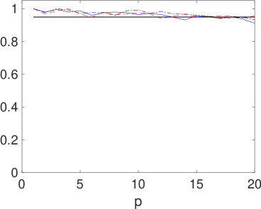
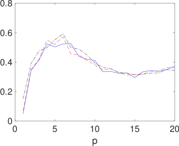
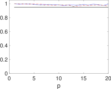
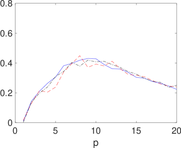
Figure 1: Frequentist coverage of the $95\%$ posterior credible interval for $p$ (left) and square root of relative mean squared error of the estimator of $p$ (right) for the SEPD. The simulations are for $\alpha=0.2$ (blue continuous line), $\alpha=0.5$ (red dashed line) and $\alpha=0.8$ (black dotted line), and for $T=100$ (top), $T=250$ (bottom).

As the yielded posterior distribution for the parameters is not analytically tractable, it is necessary to adopt Markov Chain Monte Carlo (MCMC) methods. In particular, we have implemented a Metropolis within Gibbs sampler. For each of the above $250$ samples, we have run $20000$ iterations of the MCMC algorithm and discarded the first $5000$ iterations as burn-in period. The results of the frequentist analysis of the posterior of $p$ are plotted in Figure 1. Examining the coverage, we note that the samples with $T=100$ have a frequency closer to the nominal value (i.e. 95%) compared to the samples with $T=250$; this is more obvious for relatively large values of $p$. The MSE behaves in line with other frequentist studies for tail parameters (such as for the Student-$t$ and the skewed Student-$t$), with a smaller index value for larger sample size (as expected). Finally, we note that the effect of $\alpha$ on the frequentist performances is negligible.

To have a feeling of the complete inferential procedure, we show how all the parameters of a model are estimated. In particular, we consider an autoregressive model with one lag, $\phi_{1}=-0.5$. The error terms are assumed to have an SEPD with $\sigma=1$, $\alpha=0.23$ and $p=9$. We have drawn a sample of size $T=300$ from the model and implemented the MCMC procedure described above. In Figure 2 we show the posterior chain and histogram for parameters $\alpha$, $\phi_{1}$, $p$ and $\sigma$. The corresponding posterior mean, median and 95% credible interval are reported in Table 1. We note that the true parameter values are well contained in the corresponding posterior credible interval.

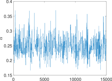
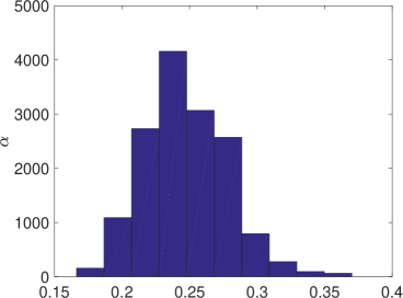
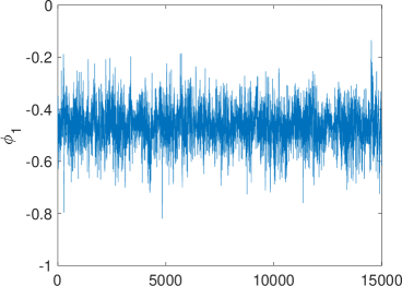
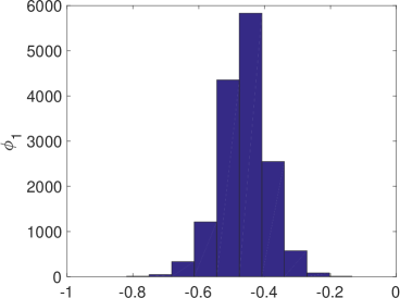
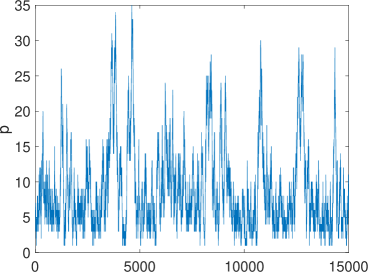
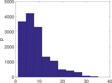
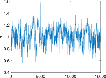
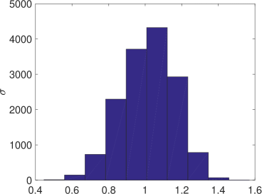
Figure 2: Sample chains (left panels) and histograms of the posterior distributions (right panels) of the parameters for the simulated data from the SEPD with $\alpha=0.23$, $\phi_{1}=-0.5$, $p=9$, $\sigma=1$ and $T=300$.

Parameter	Mean	Median	$95\%$ C.I.
$\alpha$	0.2476	0.2456	(0.1917, 0.3125)
$\phi_{1}$	-0.4612	-0.4614	(-0.6147, -0.3187)
$p$	8.94	8	(2, 25)
$\sigma$	1.0179	1.0232	(0.7104,1.2751)

Table 1: Summary statistics of the posterior distributions for the parameters of the simulated data from an SEPD with $\alpha=0.23$, $\phi_{1}=-0.5$, $p=9$, $\sigma=1$ and $T=300$.

4.2 SGLD simulation study

To study the performance of the loss-based prior for the tail parameter $p$ of the SGLD, as anticipated, we consider a linear regression model where the error terms have the above distribution. That is,

$$y_{i}=\beta_{0}+\beta_{1}x_{i}+\varepsilon_{i},\qquad i=1,\ldots,n,$$ (13)

where, for the purpose of this simulation, we have set $\beta_{0}=1.5$, $\beta_{1}=-1$ and $\varepsilon_{i}\sim SGLD(\alpha,p,\mu,\sigma)$. We select 250 random samples from the above model (13) for each scenario determined by $p=1,\ldots,20$, $\alpha=\{0.3,0.5,0.8\}$ and $n=30,100$. The scale parameter $\sigma$ has been fixed to 1. The simulation study has been performed by considering a loss-based prior on $p$, the Jeffreys prior for the skewness parameter, $\pi(\alpha)\sim\mbox{Be}(1/2,1/2)$, and for the scale parameter, $\pi(\sigma)\propto 1/\sigma$ (as discussed in Section 3.2). For $\beta_{0}$ and $\beta_{1}$ we have used the Zellner g-prior (Zellner,, 1986) with $g=n$, which is a bivariate normal with zero means and covariance matrix $\Sigma=n(X^{\prime}X)^{-1}$, where $X=(1,x_{1i})$.

For this model as well the posterior distribution is analytically intractable. Therefore, we have implemented an MCMC procedure (Metropolis within Gibbs samples) with 10000 iterations and a burn-in period of 5000 iterations. The frequentist analysis of the posterior for $p$ is shown in Figure 3. The coverage of the posterior 95% credible interval appears to be very similar whether we consider the different values of the skewness parameter $\alpha$ or the sample size. For what it concerns the MSE, we note some differences when the sample size is 30, although these are most certainly due to the relatively small amount of information about $p$ contained in the sample. This difference vanishes for $n=100$.

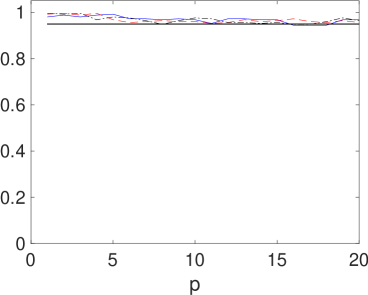
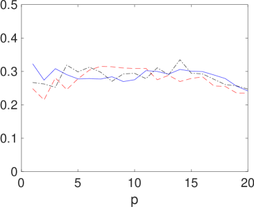
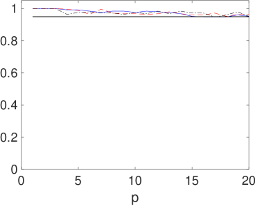
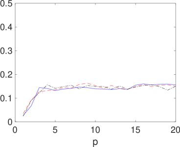
Figure 3: Frequentist coverage of the $95\%$ credible intervals for $p$ (left) and square root of relative mean squared error of the estimator of $p$ (right) for the SGLD. The simulations are for $\alpha=0.2$ (blue continuous line), $\alpha=0.5$ (red dashed line) and $\alpha=0.8$ (black dotted line), and for $n=30$ (top), $n=100$ (bottom).

Similarly to the study of the SEPD model, we report the complete inferential procedure for a single sample drawn from the model in (13), where we have set $\beta_{0}=-2.5$, $\beta_{1}=3$, $\alpha=0.23$, $p=9$ and $\sigma=1$. We run an MCMC procedure with $30.000$ iterations and a burn-in period of $5.000$ iterations. The posterior chains and histograms are plotted in Figure 4, with the corresponding posterior statistics reported in Table 2. We note that the posterior means and medians give an excellent point representation of the true parameter values, and that the posterior credible intervals contain the above true values giving a high level accuracy of the estimates.

Parameter	Mean	Median	$95\%$ C.I.
$\alpha$	0.1363	0.136	(0.1155,0.1615)
$\beta_{0}$	-2.5396	-2.54	(-2.5775, -2.4964)
$\beta_{1}$	3.0048	3.0041	(2.9639, 3.0494)
$p$	8.9295	9	(8, 10)

Table 2: Summary statistics of the posterior distributions for the parameters of the simulated data from an SGLD with $\alpha=0.13$, $\beta_{0}=-2.5$, $\beta_{1}=3$, $p=9$ and $n=300$.

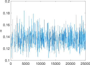
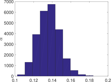
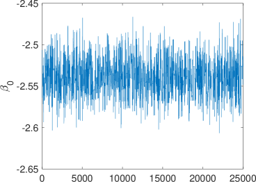
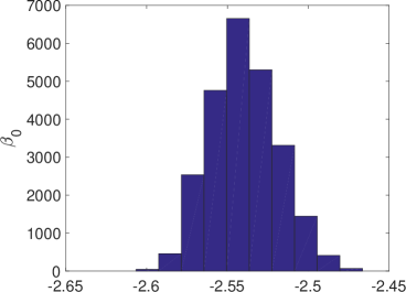
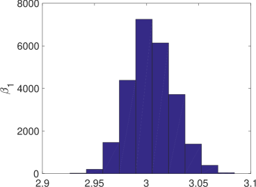
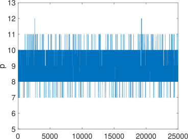
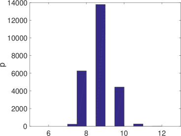
Figure 4: panels) of the parameters for the simulated data from the SGLD with $\alpha=0.13$, $\beta_{0}=-2.5$, $\beta_{1}=3$, $p=9$ and $n=300$.

5 Real Data Analysis

In this section, we present two different examples with publicly available data to illustrate how the loss-based prior for the tail parameter $p$ performs. In the first example we analyse the Nordpool Electricity prices by means of an autoregressive model with error terms distributed as a skewed exponential power, while in the second example we apply a linear regression model with error terms distributed as a skewed generalised logistic to Small Cell Cancer data.

5.1 Nordpool Electricity Prices Data

We use monthly prices (in level) to estimate models for electricity traded (Bottazzi and Secchi,, 2011; Trindade et al.,, 2010) in Nordpool countries: in particular, Finland and Denmark. The prices, which have been obtained directly from the corresponding power exchanges, are plotted in Figure 5. Note that, for Denmark, we have averaged the two hourly zonal prices from Nordpool. The data is considered as the growth rate, meaning that we model the standardised first differences.

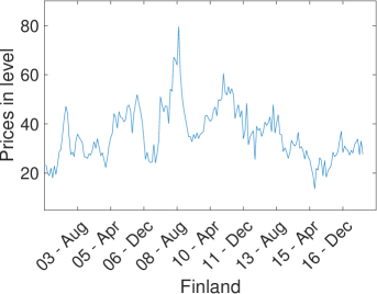
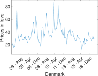
Figure 5: Monthly electricity prices (in level) for Finland (top) and Denmark (bottom) from January 2003 to December 2017.

Finally, of the $T=180$ observation points, we use the first ten years as estimation sample and the last five years as forecast evaluation period.

The data is modelled with a univariate autoregressive model with one lag, where the error terms are SEPD. The results of the analysis are based on one-step-ahead forecasting process with a rolling window approach of 10 years for both the countries, and we have a forecast evaluation period of 60 observations (from January 2013 to December 2017). Following the results in Section 4, we run the estimation procedure through Gibbs sampling with a burn-in of $5.000$ iterations and for the forecasting procedure we use the remaining $15.000$ iterations.

We assess the goodness of our forecasts using different point and density metrics. For point forecasts, we use the root mean square errors (RMSEs) for the monthly prices as follows:

$$\mbox{RMSE}=\sqrt{\frac{1}{T-R}\sum_{t=R}^{T-1}\left(\hat{y}_{t+1|t}-y_{t+1|t}\right)^{2}},$$ (14)

where $T$ is the number of observations, $R$ is the length of the rolling window and $\hat{y}_{t+1|t}$ are the price forecasts.

To evaluate density forecasts, we use both the average log predictive score and the average continuous ranked probability score (CRPS). The log predictive score is computed as follows (see Geweke and Amisano, (2010))

$$s_{t}(y_{t+1})=\log{\left(f(y_{t+1}|I_{t}\right)},$$

where $f(y_{t+1}|I_{t})$ is the predictive density for $y_{t+1}$ constructed using information up to time $t$. In addition, following Gneiting and Raftery, (2007) and Gneiting and Ranjan, (2011), we also compute the continuous ranked probability score, which has some advantages with respect to the log-score. In fact, it is less sensitive to outliers. It can be computed as follows:

$$\mbox{CRPS}_{t}(y_{t+1})=\int_{-\infty}^{\infty}\left(F(z)-\mathbb{I}\{y_{t+1}\leq z\}\right)^{2}dz=E_{f}|Y_{t+1}-y_{t+1}|-0.5E_{f}|Y_{t+1}-Y^{\prime}_{t+1}|,$$ (15)

where $F$ denotes the cumulative distribution function associated with the predictive density $f$, $\mathbb{I}\{y_{t+1}\leq z\}$ denotes an indicator function taking value $1$ if $y_{t+1}\leq z$ and $0$ otherwise, and $Y_{t+1}$ and $Y^{\prime}_{t+1}$ are independent random draws from the posterior predictive density.

In Table 3, we report the RMSEs, average log-scores and average CRPS for the benchmark model, which is referred as the AR model with frequentist estimation. We compare the results from the Ordinary Least Squares (OLS) benchmark with the results obtained from the Bayesian AR with Normal error and our model based on SEPD errors. We also report the ratios of each model RMSE (average CRPS) to the baseline AR model, such that entries less than 1 indicate that the given model yields forecasts more accurate than those from the baseline. For the log-score, positive differences in score indicate that the given model outperforms the baseline.

	Forecast	OLS	Bayesian Normal	SEPD error
Finland	RMSE	0.749	1.003	1.022
	log-score	-1.334	0.090	0.106
	CRPS	0.491	0.899	0.891
Denmark	RMSE	0.541	1.001	1.021
	log-score	-1.143	0.013	0.165
	CRPS	0.355	0.990	0.918

Table 3: Point (RMSE) and density forecast (average log predictive score and average CRPS) for Finland and Denmark. The first column (OLS) refers to the benchmark model and shows the values of the RMSE, average log predictive score and average CRPS. The second (Bayesian Normal) and third (SEPD error) columns refer to the RMSE ratios, score differences and CRPS ratios with respect to the benchmark model (OLS).

For both Finland and Denmark the point forecast appears to be worse than the benchmark. This is more obvious for the AR model with SEPD errors, although the values are not far from one. There is a noticeable improvement, in using SEPD errors, when we focus on density forecast. In fact, considering the log-score, we have a improvement in considering SEPD (instead of normal) errors from 0.090 to 0.106 for Finland, and a more obvious improvement from 0.013 to 0.165 for Denmark.

5.2 Small Cell Cancer Data

In this second example we illustrate the loss-based prior for the tail parameter $p$ when we employ a linear regression model with SGLD errors. The data has been obtained from Ying et al., (1995), where a lung cancer study with two differente types of treatment has been performed. In particular, the study contained $n=121$ survival times (in log-days) of patients with small cell lung cancer (SCLC) to whom were administrated two different therapies. A treatment consisted of a combination of etoposide (E) and cisplatin (P) in any order. The patient were split into two treatment groups: treatment A ($62$ patients), where the therapy consisted in administering P followed by E; treatment B ($59$ patients), where the therapy consisted in administering E followed by P. We regress the survival time on the following two covariates: the entry age (in years) and a dummy variable identifying the type of treatment (A or B).

The estimation of the parameters of the regression model has been done through Monte Carlo methods, as described in Section 4, with 50000 iterations and a burn-in period of 10000 iterations. Figure 6 shows the histograms of the posterior distributions for the parameters, while in Table 4 we have the corresponding posterior statistics.

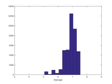
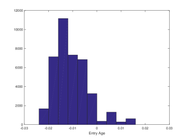
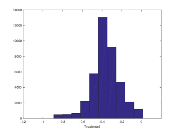
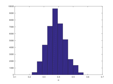
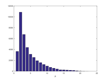
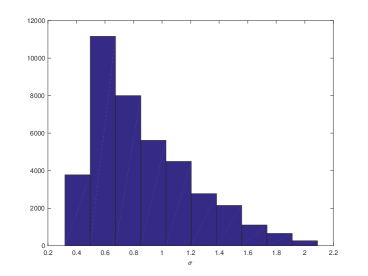
Figure 6: Posterior histograms for the parameters of the regression model with SGLD errors for the SCLC study.

The estimated intercept of the regression model, represented by the posterior median, is similar to the result in Rubio and Yu, (2017), that is 6.69. Similar considerations can be drawn for the coefficient of the entry age, which is very small and with a credible interval containing the zero; this last result supports the conclusion that the effect of the entry age on the survival time is negligible. However, the treatment appear to have a significant (negative) effect on the survival time, both under the estimated model and the results in Rubio and Yu, (2017). For the scale parameter $\sigma$, we again see agreement between the SEPD regression and the results of the above authors, although our credible interval is larger. It is not possible to perform a direct comparison of the estimated asymmetry, but in both case the value shows a clear positive skewness. Finally, our inferential procedure suggests that the data exhibit heavy tails, as indicated by the posterior median of $p=3$.

Parameter	Mean	Median	$95\%$ C.I.	Rubio & Yu
Intercept	6.8438	6.9059	(5.6692, 7.4672)	6.690
Entry age	-0.0105	-0.0117	(-0.0216, 0.0079)	-0.009
Treatment	-0.3637	-0.3611	(-0.7161, -0.0552)	-0.446
$\alpha$	0.3837	0.3814	(0.2717, 0.5116)	-0.395 ($\gamma$)
$p$	4.5349	3	(1, 14)	NA
$\sigma$	0.8630	0.7771	(0.3649, 1.7209)	0.650

Table 4: SCLC Lung Cancer data: Posterior mean, posterior median and $95\%$ credible interval of the posterior for the regression model parameters. The last column to the right reports the posterior means from Rubio and Yu, (2017), where the skewness parameter is represented by $\gamma\in(-1,1)$ expressing positive skewness for values smaller than 0.

6 Discussion

We have illustrated an objective Bayesian approach in the estimation of the tail parameter in two particular distributions: the skewed exponential power distribution (SEPD) and the skewed generalised logistic distribution (SGLD). This represents a new application of the well-known loss-based prior (Villa and Walker,, 2015), where information theoretical considerations are used to derive minimally informative prior distributions. The SEPD and the SGLD are part of the wider family of two-piece location-scale distribution and allow to entangle skewness and tail fatness in one single probability distribution. Therefore, they represent an appealing modeling solution in scenarios where such behaviours are exhibited by the data, such as in financial applications and survival analysis. We illustrate the properties of the loss-based prior for the tail parameter of the above distributions by performing a thorough simulation study and analysis two real data sets. Furthermore, we show how the SEPD and SGLD can be used to model error terms in complex modeling situations, such as the error terms of autoregressive process for time series and error terms for linear regression models.

A Proofs

Proof of Theorem 3.1.

Note that,

$$D_{\text{KL}}\left(f_{p}^{\alpha,\mu,\sigma}||f_{p^{\prime}}^{\alpha,\mu,\sigma}\right)=D_{\leq}\left(f_{p}^{\alpha,\mu,\sigma}||f_{p^{\prime}}^{\alpha,\mu,\sigma}\right)+D_{>}\left(f_{p}^{\alpha,\mu,\sigma}||f_{p^{\prime}}^{\alpha,\mu,\sigma}\right),$$

where the above Kullback–Leibler divergences are:

$$D_{\leq}\left(f_{p}^{\alpha,\mu,\sigma}||f_{p^{\prime}}^{\alpha,\mu,\sigma}\right)=\int_{-\infty}^{\mu}f_{p}^{\alpha,\mu,\sigma}(y)\log{\left\{\frac{f_{p}^{\alpha,\mu,\sigma}(y)}{f_{p^{\prime}}^{\alpha,\mu,\sigma}(y)}\right\}}\,dy$$

and

$$D_{\geq}\left(f_{p}^{\alpha,\mu,\sigma}||f_{p^{\prime}}^{\alpha,\mu,\sigma}\right)=\int_{\mu}^{\infty}f_{p}^{\alpha,\mu,\sigma}(y)\log{\left\{\frac{f_{p}^{\alpha,\mu,\sigma}(y)}{f_{p^{\prime}}^{\alpha,\mu,\sigma}(y)}\right\}}\,dy.$$

Focusing on the first term, we have that:

$$\begin{split}D_{\leq}\left(f_{p}^{\alpha,\mu,\sigma}||f_{p^{\prime}}^{\alpha,\mu,\sigma}\right)&=\int_{-\infty}^{\mu}f_{p}^{\alpha,\mu,\sigma}(y)\log{\left\{\frac{f_{p}^{\alpha,\mu,\sigma}(y)}{f_{p^{\prime}}^{\alpha,\mu,\sigma}(y)}\right\}}\,dy\\ &=\int_{-\infty}^{\mu}\frac{1}{\sigma}f_{p}\left(\frac{y-\mu}{2\alpha\sigma}\right)\log{\left\{\frac{f_{p}\left(\frac{y-\mu}{2\alpha\sigma}\right)}{f_{p^{\prime}}\left(\frac{y-\mu}{2\alpha\sigma}\right)}\right\}}\,dy\\ \ \end{split}$$

where the last equality follows from (8). By performing the change of variable $x=\frac{y-\mu}{2\alpha\sigma}$, we get

$$\begin{split}D_{\leq}\left(f_{p}^{\alpha,\mu,\sigma}||f_{p^{\prime}}^{\alpha,\mu,\sigma}\right)&=2\alpha\int_{-\infty}^{0}f_{p}(x)\log{\left\{\frac{f_{p}(x)}{f_{p^{\prime}}(x)}\right\}}\,dx\\ &=2\alpha D_{\leq}(f_{p}||f_{p^{\prime}}).\\ \end{split}$$

For the models under consideration, i.e. the SEPD and the SGLD, $f_{p}=f_{p}^{\alpha=0.5,\mu=0,\sigma=1}$ and $f_{p^{\prime}}=f_{p^{\prime}}^{\alpha=0.5,\mu=0,\sigma=1}$. Therefore,

$$D_{\leq}\left(f_{p}^{\alpha,\mu,\sigma}||f_{p^{\prime}}^{\alpha,\mu,\sigma}\right)=2\alpha D_{\leq}\left(f_{p}^{\alpha=0.5,\mu=0,\sigma=1}||f_{p^{\prime}}^{\alpha=0.5,\mu=0,\sigma=1}\right).$$

Similarly,

$$D_{>}\left(f_{p}^{\alpha,\mu,\sigma}||f_{p^{\prime}}^{\alpha,\mu,\sigma}\right)=2(1-\alpha)D_{>}\left(f_{p}^{\alpha=0.5,\mu=0,\sigma=1}||f_{p^{\prime}}^{\alpha=0.5,\mu=0,\sigma=1}\right).$$

Note that,

$$D_{\leq}\left(f_{p}^{\alpha=0.5,\mu=0,\sigma=1}||f_{p^{\prime}}^{\alpha=0.5,\mu=0,\sigma=1}\right)=D_{>}\left(f_{p}^{\alpha=0.5,\mu=0,\sigma=1}||f_{p^{\prime}}^{\alpha=0.5,\mu=0,\sigma=1}\right).$$

As a consequence,

$$\begin{split}D_{KL}\left(f_{p}^{\alpha=0.5,\mu=0,\sigma=1}||f_{p^{\prime}}^{\alpha=0.5,\mu=0,\sigma=1}\right)&=2D_{\leq}\left(f_{p}^{\alpha=0.5,\mu=0,\sigma=1}||f_{p^{\prime}}^{\alpha=0.5,\mu=0,\sigma=1}\right)\\ &=2D_{>}\left(f_{p}^{\alpha=0.5,\mu=0,\sigma=1}||f_{p^{\prime}}^{\alpha=0.5,\mu=0,\sigma=1}\right).\end{split}$$

Therefore, by using the above identity, we can conclude the proof:

$$D_{\text{KL}}\left(f_{p}^{\alpha,\mu,\sigma}||f_{p^{\prime}}^{\alpha,\mu,\sigma}\right) =D_{\leq}\left(f_{p}^{\alpha,\mu,\sigma}||f_{p^{\prime}}^{\alpha,\mu,\sigma}\right)+D_{>}\left(f_{p}^{\alpha,\mu,\sigma}||f_{p^{\prime}}^{\alpha,\mu,\sigma}\right)$$

$$=2\alpha D_{\leq}\left(f_{p}^{\alpha=0.5,\mu=0,\sigma=1}||f_{p^{\prime}}^{\alpha=0.5,\mu=0,\sigma=1}\right)+$$

$$\hskip 56.9055pt+2(1-\alpha)D_{>}\left(f_{p}^{\alpha=0.5,\mu=0,\sigma=1}||f_{p^{\prime}}^{\alpha=0.5,\mu=0,\sigma=1}\right)$$

$$=\alpha D_{KL}\left(f_{p}^{\alpha=0.5,\mu=0,\sigma=1}||f_{p^{\prime}}^{\alpha=0.5,\mu=0,\sigma=1}\right)+$$

$$\hskip 56.9055pt+(1-\alpha)D_{KL}\left(f_{p}^{\alpha=0.5,\mu=0,\sigma=1}||f_{p^{\prime}}^{\alpha=0.5,\mu=0,\sigma=1}\right)$$

$$=D_{KL}\left(f_{p}^{\alpha=0.5,\mu=0,\sigma=1}||f_{p^{\prime}}^{\alpha=0.5,\mu=0,\sigma=1}\right).$$

∎

Proof of Theorem 3.2.

Using the probability density function displayed in equation (3), we have that:

$$D_{KL}\left(f_{p}^{\alpha=0.5,\mu=0,\sigma=1}||f_{p^{\prime}}^{\alpha=0.5,\mu=0,\sigma=1}\right) =\int_{-\infty}^{\infty}K(p)e^{-\frac{1}{p}\left|z\right|^{p}}\log{\left\{\frac{K(p)e^{-\frac{1}{p}\left|z\right|^{p}}}{K(p^{\prime})e^{-\frac{1}{p^{\prime}}\left|z\right|^{p^{\prime}}}}\right\}}\,dz$$

$$=2\int_{0}^{\infty}K(p)e^{-\frac{1}{p}z^{p}}\log{\left\{\frac{K(p)e^{-\frac{1}{p}z^{p}}}{K(p^{\prime})e^{-\frac{1}{p^{\prime}}z^{p^{\prime}}}}\right\}}\,dz$$

$$=2\left[\log{K(p)}-\log{K(p^{\prime})}\right]K(p)\int_{0}^{\infty}e^{-\frac{1}{p}z^{p}}\,dz$$

$$-2\frac{K(p)}{p}\int_{0}^{\infty}e^{-\frac{1}{p}z^{p}}z^{p}\,dz+2\frac{K(p)}{p^{\prime}}\int_{0}^{\infty}e^{-\frac{1}{p}z^{p}}z^{p^{\prime}}\,dz.$$ (A.1)

From 3.478.1 of Gradshteyn and Ryzhik, (2007),

$$\int_{0}^{\infty}x^{\nu-1}e^{-\mu x^{p}}\,dx=\frac{1}{p}\mu^{-\nu/p}\Gamma\left(\frac{\nu}{p}\right),$$

we have that equation A.1 becomes:

$$D_{KL}\left(f_{p}^{\alpha=0.5,\mu=0,\sigma=1}||f_{p^{\prime}}^{\alpha=0.5,\mu=0,\sigma=1}\right) =2\left[\log{\frac{K(p)}{K(p^{\prime})}}\right]\frac{K(p)}{p}\left(\frac{1}{p}\right)^{-\frac{1}{p}}\Gamma\left(\frac{1}{p}\right)-2\frac{K(p)}{p^{2}}\left(\frac{1}{p}\right)^{-\frac{(p+1)}{p}}\Gamma\left(\frac{p+1}{p}\right)$$

$$+2\frac{K(p)}{p^{\prime}}\frac{1}{p}\left(\frac{1}{p}\right)^{-\frac{(p^{\prime}+1)}{p}}\Gamma\left(\frac{p^{\prime}+1}{p}\right)$$

$$=\log{K(p)}-\log{K(p^{\prime})}-p^{-1}+\frac{p^{\frac{p^{\prime}}{p}}}{p^{\prime}}\frac{\Gamma\left(\frac{p^{\prime}+1}{p}\right)}{\Gamma\left(\frac{1}{p}\right)}.$$

In conclusion, following theorem 3.1, the Kullback-Leibler divergence has the form

$$D_{\text{KL}}\left(f_{p}^{\alpha,\mu,\sigma}||f_{p^{\prime}}^{\alpha,\mu,\sigma}\right)=\log{K(p)}-\log{K(p^{\prime})}-p^{-1}+\frac{p^{\frac{p^{\prime}}{p}}}{p^{\prime}}\frac{\Gamma\left(\frac{p^{\prime}+1}{p}\right)}{\Gamma\left(\frac{1}{p}\right)}.$$

∎

Proof of Theorem 3.3.

Using the probability density function displayed in equation (5), we have that:

$$D_{KL}\left(f_{p}^{\alpha=0.5,\mu=0,\sigma=1}||f_{p^{\prime}}^{\alpha=0.5,\mu=0,\sigma=1}\right) =\int_{-\infty}^{\infty}\frac{e^{-px}}{B(p,p)(1+e^{-x})^{2p}}\log{\left[\frac{B(p^{\prime},p^{\prime})}{B(p,p)}\frac{e^{-px}/(1+e^{-x})^{2p}}{e^{-p^{\prime}x}/(1+e^{-x})^{2p^{\prime}}}\right]}\,dx=$$

$$=\int_{0}^{1}\frac{1}{B(p,p)}t^{p-1}(1-t)^{p-1}\log{\left[\frac{B(p^{\prime},p^{\prime})}{B(p,p)}\frac{t^{p}(1-t)^{p}}{t^{p^{\prime}}(1-t)^{p^{\prime}}}\right]}\,dt,$$

where $t=S(x)$, $dt=s(x)dx$ and $S(x)$ and $s(x)$ are the cumulative distribution and the probability distribution function of the logistic distribution, respectively. Hence, we can extend the Kullback–Leibler divergence as

$$D_{KL}\left(f_{p}^{\alpha=0.5,\mu=0,\sigma=1}||f_{p^{\prime}}^{\alpha=0.5,\mu=0,\sigma=1}\right) =\log{\left[\frac{B(p^{\prime},p^{\prime})}{B(p,p)}\right]}+\frac{(p-p^{\prime})}{B(p,p)}\int_{0}^{1}t^{p-1}(1-t)^{p-1}\log{(t)}\,dt$$

$$+\frac{(p-p^{\prime})}{B(p,p)}\int_{0}^{1}t^{p-1}(1-t)^{p-1}\log{(1-t)}\,dt$$

$$=\log{\left[\frac{B(p^{\prime},p^{\prime})}{B(p,p)}\right]}+\frac{2(p-p^{\prime})}{B(p,p)}\int_{0}^{1}t^{p-1}(1-t)^{p-1}\log{(t)}\,dt.$$ (A.2)

In conclusion, from 4.253.1 of Gradshteyn and Ryzhik, (2007)

$$\int_{0}^{1}t^{p-1}(1-t)^{p-1}\log{(t)}dt=B(p,p)\left[\psi(p)-\psi(2p)\right],$$

where $\psi(p)$ is the digamma function, the Kullback–Leibler divergence represented in equation A.2 have the following form

$$D_{KL}\left(f_{p}^{\alpha=0.5,\mu=0,\sigma=1}||f_{p^{\prime}}^{\alpha=0.5,\mu=0,\sigma=1}\right) =\log{\left[\frac{B(p^{\prime},p^{\prime})}{B(p,p)}\right]}+2(p-p^{\prime})\left[\psi(p)-\psi(2p)\right].$$

∎

B Comparison of the Kullback–Leibler Divergence for different distributions

p	$D_{\text{KL}}\left(f_{p}^{\alpha,\mu,\sigma}||f_{p-1}^{\alpha,\mu,\sigma}\right)$	$D_{\text{KL}}\left(f_{p}^{\alpha,\mu,\sigma}||f_{p+1}^{\alpha,\mu,\sigma}\right)$			p	$D_{\text{KL}}\left(f_{p}^{\alpha,\mu,\sigma}||f_{p-1}^{\alpha,\mu,\sigma}\right)$	$D_{\text{KL}}\left(f_{p}^{\alpha,\mu,\sigma}||f_{p+1}^{\alpha,\mu,\sigma}\right)$
2	7.2093$\times 10^{-02}$	5.9144$\times 10^{-02}$			17	6.1438 $\times 10^{-04}$	6.3413$\times 10^{-04}$
3	2.7675$\times 10^{-02}$	2.6462$\times 10^{-02}$			18	5.3875 $\times 10^{-04}$	5.5578 $\times 10^{-04}$
4	1.4752$\times 10^{-02}$	1.4759$\times 10^{-02}$			19	4.7558 $\times 10^{-04}$	4.9036 $\times 10^{-04}$
5	9.1321$\times 10^{-03}$	9.3019$\times 10^{-03}$			20	4.2233 $\times 10^{-04}$	4.3523 $\times 10^{-04}$
6	6.1732$\times 10^{-03}$	6.3402$\times 10^{-03}$			21	3.7707 $\times 10^{-04}$	3.8840 $\times 10^{-04}$
7	4.4262$\times 10^{-03}$	4.5646$\times 10^{-03}$			22	3.3833 $\times 10^{-04}$	3.4833 $\times 10^{-04}$
8	3.3117$\times 10^{-03}$	3.4223$\times 10^{-03}$			23	3.0494 $\times 10^{-04}$	3.1381 $\times 10^{-04}$
9	2.5594$\times 10^{-03}$	2.6474$\times 10^{-03}$			24	2.7599 $\times 10^{-04}$	2.8388$\times 10^{-04}$
10	2.0292$\times 10^{-03}$	2.0997$\times 10^{-03}$			25	2.5074 $\times 10^{-04}$	2.5780 $\times 10^{-04}$
11	1.6426$\times 10^{-03}$	1.6996$\times 10^{-03}$			26	2.2861 $\times 10^{-04}$	2.3494 $\times 10^{-04}$
12	1.3527$\times 10^{-03}$	1.3994$\times 10^{-03}$			27	2.0911 $\times 10^{-04}$	2.1481 $\times 10^{-04}$
13	1.1302$\times 10^{-03}$	1.1688$\times 10^{-03}$			28	1.9186 $\times 10^{-04}$	1.9701 $\times 10^{-04}$
14	9.5616$\times 10^{-04}$	9.8838 $\times 10^{-04}$			29	1.7653 $\times 10^{-04}$	1.8120 $\times 10^{-04}$
15	8.1765 $\times 10^{-04}$	8.4480 $\times 10^{-04}$			30	1.6285 $\times 10^{-04}$	1.6710 $\times 10^{-04}$
16	7.0582 $\times 10^{-04}$	7.2889 $\times 10^{-04}$
30	1.6285 $\times 10^{-04}$	1.6710 $\times 10^{-04}$			120	5.3155 $\times 10^{-06}$	5.3800 $\times 10^{-06}$
60	3.0272 $\times 10^{-05}$	3.0829 $\times 10^{-05}$			150	3.0055 $\times 10^{-06}$	3.0370 $\times 10^{-06}$
90	1.1010 $\times 10^{-05}$	1.1169 $\times 10^{-05}$			180	1.8801 $\times 10^{-06}$	1.8975 $\times 10^{-06}$

Table B.1: Comparison of the Kullbck-Leibler divergences $D_{\text{KL}}\left(f_{p}^{\alpha,\mu,\sigma}||f_{p-1}^{\alpha,\mu,\sigma}\right)$ and $D_{\text{KL}}\left(f_{p}^{\alpha,\mu,\sigma}||f_{p+1}^{\alpha,\mu,\sigma}\right)$ for $p=2,\dots,30$ for the SEPD.

p	$D_{\text{KL}}\left(f_{p}^{\alpha,\mu,\sigma}||f_{p-1}^{\alpha,\mu,\sigma}\right)$	$D_{\text{KL}}\left(f_{p}^{\alpha,\mu,\sigma}||f_{p+1}^{\alpha,\mu,\sigma}\right)$			p	$D_{\text{KL}}\left(f_{p}^{\alpha,\mu,\sigma}||f_{p-1}^{\alpha,\mu,\sigma}\right)$	$D_{\text{KL}}\left(f_{p}^{\alpha,\mu,\sigma}||f_{p+1}^{\alpha,\mu,\sigma}\right)$
2	0.1251	0.0572			17	9.2755 $\times 10^{-04}$	8.5657 $\times 10^{-04}$
3	0.0428	0.0262			18	8.2411 $\times 10^{-04}$	7.6446 $\times 10^{-04}$
4	0.0214	0.0150			19	7.3704 $\times 10^{-04}$	6.8644 $\times 10^{-04}$
5	0.0128	0.0097			20	6.6308 $\times 10^{-04}$	6.1979 $\times 10^{-04}$
6	0.0085	0.0068			21	5.9972 $\times 10^{-04}$	5.6239 $\times 10^{-04}$
7	0.0061	0.0050			22	5.4503 $\times 10^{-04}$	5.1261 $\times 10^{-04}$
8	0.0045	0.0038			23	4.9749 $\times 10^{-04}$	4.6916 $\times 10^{-04}$
9	0.0035	0.0030			24	4.5591 $\times 10^{-04}$	4.3101 $\times 10^{-04}$
10	0.0028	0.0025			25	4.1933 $\times 10^{-04}$	3.9733 $\times 10^{-04}$
11	0.0023	0.0020			26	3.8698 $\times 10^{-04}$	3.6745 $\times 10^{-04}$
12	0.0019	0.0017			27	3.5824 $\times 10^{-04}$	3.4082 $\times 10^{-04}$
13	0.0016	0.0015			28	3.3258 $\times 10^{-04}$	3.1698 $\times 10^{-04}$
14	0.0014	0.0013			29	3.0959 $\times 10^{-04}$	2.9556 $\times 10^{-04}$
15	0.0012	0.0011			30	2.8890 $\times 10^{-04}$	2.7623 $\times 10^{-04}$
16	0.0011	0.0010
30	2.8890 $\times 10^{-04}$	2.7623 $\times 10^{-04}$			120	1.7531 $\times 10^{-05}$	1.7337 $\times 10^{-05}$
60	7.0814 $\times 10^{-05}$	6.9252 $\times 10^{-05}$			150	1.1198 $\times 10^{-05}$	1.1099 $\times 10^{-05}$
90	3.1268 $\times 10^{-05}$	3.0807 $\times 10^{-05}$			180	7.7663 $\times 10^{-06}$	7.7089 $\times 10^{-06}$

Table B.2: Comparison of the Kullbck-Leibler divergences $D_{\text{KL}}\left(f_{p}^{\alpha,\mu,\sigma}||f_{p-1}^{\alpha,\mu,\sigma}\right)$ and $D_{\text{KL}}\left(f_{p}^{\alpha,\mu,\sigma}||f_{p+1}^{\alpha,\mu,\sigma}\right)$ for $p=2,\dots,30$ for the SGLD.

C Generate samples with the SEPD and the SGLD

As described by Komunjer, (2007) and Zhu and Zinde-Walsh, (2009), the SEPD could be simulated by using the standard skewed exponential power distribution. They highlighted the following procedure:

• Generate $U\sim U(0,1)$, $W_{1}\sim Ga(1/p,1)$ and $W_{2}\sim Ga(1/p,1)$.

• Compute the following transformed variable,

  $$Z=\alpha W_{1}^{1/p}\left[\frac{\text{sign}(U-\alpha)-1}{2K(p)\Gamma(1+1/p)}\right]+(1-\alpha)W_{2}^{1/p}\left[\frac{\text{sign}(U-\alpha)+1}{2K(p)\Gamma(1+1/p)}\right].$$ (C.1)

  where $\text{sign}(x)=1$ if $x>0$, $\text{sign}(x)=-1$ if $x<0$ and $\text{sign}(x)=0$ if $x=0$.

The above procedure generates an observation from the SEPD with $\mu=0$, $\sigma=1$. We can obtain a SEPD with different $\mu$ and $\sigma$ by simply multiplying $Z$ by the scale parameter and adding the location parameter.

Simulating from the SGLD follows a similar procedure. In particular,

• Generate $U\sim U(0,1)$, $W_{1}$ and $W_{2}$ from the distribution displayed in (4).

• Compute the following transformed variable,

  $$Z=\alpha|W_{1}|\left[\text{sign}(U-\alpha)-1\right]+(1-\alpha)|W_{2}|\left[\text{sign}(U-\alpha)+1\right],$$ (C.2)

  where $\text{sign}(x)=1$ if $x>0$, $\text{sign}(x)=-1$ if $x<0$ and $\text{sign}(x)=0$ if $x=0$.

The above procedure generates an observation from the SGLD with $\mu=0$, $\sigma=1$. We can obtain a SGLD with different $\mu$ and $\sigma$ by simply multiplying $Z$ by the scale parameter and adding the location parameter.

References

- Azzalini, (1985) Azzalini, A. (1985). A class of distributions which includes the normal ones. Scandinavian Journal of Statistics, 12(2):171–178.
- Berger et al., (2009) Berger, J. O., Bernardo, J. M., and Sun, D. (2009). The Formal definition of reference priors. Annals of Statistics, 37(2):905–938.
- Berk, (1966) Berk, R. (1966). Limiting behaviour of posterior distributions when the model is incorrect. Ann. of Math. Statist., 37:51–58.
- Bottazzi and Secchi, (2011) Bottazzi, G. and Secchi, A. (2011). A new class of asymmetric exponential power densities with applications to economics and finance. Industrial and Corporate Change, 20(4):991–1030.
- Conejo et al., (2005) Conejo, Contreras, Espínola, and Plazas (2005). Forecasting electricity prices for a day-ahead poolbased electric energy market. International Journal of Forecasting, 21(3):435–462.
- Fernandez and Steel, (1998) Fernandez, C. and Steel, M. F. J. (1998). On Bayesian modeling of fat tails and skewness. Journal of the American Statistical Association, 93:359–371.
- Geweke and Amisano, (2010) Geweke, J. and Amisano, G. (2010). Comparing and evaluating Bayesian predictive distributions of asset returns. International Journal of Forecasting, 26(2):216–230.
- Gneiting and Raftery, (2007) Gneiting, T. and Raftery, A. (2007). Strictly proper scoring rules, prediction and estimation. Journal of American Statistical Association, 102(477):359–378.
- Gneiting and Ranjan, (2011) Gneiting, T. and Ranjan, R. (2011). Comparing density forecasts using threshold and quantile weighted proper scoring rules. Journal of Business and Economic Statistics, 29(3):411–422.
- Gradshteyn and Ryzhik, (2007) Gradshteyn, I. and Ryzhik, I. (2007). Table of Integrals, Series and Products. Academic Press.
- Harvey and Lange, (2016) Harvey, A. and Lange, R.-J. (2016). Volatility modeling with a generalized t distribution. Journal of Time Series Analysis, 38(2):175–190.
- Jeffreys, (1961) Jeffreys, H. (1961). Theory of Probability. Oxford University Press.
- Jones, (2004) Jones, M. C. (2004). Families of distributions arising from distribution of order statistics. Test, 13(1):1–43.
- Komunjer, (2007) Komunjer, I. (2007). Asymmetric power distribution: theory and applications to risk measurement. Journal of Applied Econometrics, 22:891–921.
- Kozubowski and Podgorski, (2001) Kozubowski, T. J. and Podgorski, K. (2001). Asymmetric Laplace laws and modeling financial data. Mathematical and Computer Modelling, 34(9-11):1003–1021.
- Leisen et al., (2017) Leisen, F., Marin, J. M., and Villa, C. (2017). Objective Bayesian modeling of insurance risks with the skew student-t distribution. Applied Stochastic Models in Business and Industry, 33(2):136–151.
- Maciejowska and Weron, (2015) Maciejowska, K. and Weron, R. (2015). Forecasting of daily electricity prices with factor models: utilizing intra-day and inter-zone relationships. Computational Statistics, 30(3):805–819.
- Merhav and Feder, (1998) Merhav, N. and Feder, M. (1998). Universal prediction. IEEE Trans. Inf. Theory, 44:2124–2147.
- Misiorek et al., (2006) Misiorek, A., Trueck, S., and Weron, R. (2006). Point and interval forecasting of spot electricity prices: linear vs. non-linear time series models. Studies in Nonlinear Dynamics & Econometrics, 10(2).
- Mudholkar and Hutson, (2000) Mudholkar, G. S. and Hutson, A. D. (2000). The epsilon-skew-normal distribution for analyzing near-normal data. Journal of Statistical Planning and Inference, 83:291–309.
- Nowotarski and Weron, (2018) Nowotarski, J. and Weron, R. (2018). Recent advances in electricity price forecasting: A review of probabilistic forecasting. Renewable and Sustainable Energy Reviews, 81(Part 1):1548 – 1568.
- Rubio and Steel, (2011) Rubio, F. J. and Steel, M. F. J. (2011). Inference for grouped data with a truncated skew-Laplace distribution. Computational Statistics and Data Analysis, 55(12):3218–3231.
- Rubio and Steel, (2014) Rubio, F. J. and Steel, M. F. J. (2014). Inference in Two-Piece Location-Scale models with Jeffreys priors. Bayesian Analysis, 9(1):1–22.
- Rubio and Yu, (2017) Rubio, F. J. and Yu, K. (2017). Flexible objective bayesian linear regression with applications in survival analysis. Journal of Applied Statistics, 44:798–810.
- Trindade et al., (2010) Trindade, A. A., Zhu, Y., and Andrews, B. (2010). Time series models with asymmetric laplace innovations. Journal of Statistical Computation and Simulation, 80(12):1317–1333.
- Tu et al., (2016) Tu, S., Wang, M., and Sun, X. (2016). Bayesian analysis of two-piece location–scale models under reference priors with partial information. Computational Statistics and Data Analysis, 96:133–144.
- Villa and Walker, (2015) Villa, C. and Walker, S. G. (2015). An Objective approach to prior mass function for discrete parameter spaces. Journal of the American Statistical Association, 110(511):1072–1082.
- Weron, (2014) Weron, R. (2014). Electricity price forecasting: A review of the state-of-the-art with a look into the future. International Journal of Forecasting, 30(4):1030 – 1081.
- Ying et al., (1995) Ying, Z., Jung, S., and Wei, L. (1995). Survival analysis with median regression models. Journal of American Statistical Association, 90(178-184).
- Zellner, (1986) Zellner, A. (1986). On assessing prior distributions and Bayesian regression analysis with g-prior distributions. Bayesian inference and Decision techniques: Essays in Honor of Bruno De Finetti, 6:233–243.
- Zhao et al., (2007) Zhao, X., Zhang, H., Lai, K. K., and Wang, S. (2007). A method for evaluating mutual funds performance based on asymmetric Laplace distribution and DEA approach. System Engineering Theory and Practice, 27(10):1–10.
- Zhu and Galbraith, (2010) Zhu, D. and Galbraith, J. W. (2010). A generalized asymmetric Student-t distribution with applications to financial econometrics. Journal of Applied Econometrics, 157:197–305.
- Zhu and Galbraith, (2011) Zhu, D. and Galbraith, J. W. (2011). Modeling and forecasting expected shortfall with the generalized asymmetric student-t and asymmetric exponential power distributions. Journal of Empirical Finance, 18:765–778.
- Zhu and Zinde-Walsh, (2009) Zhu, D. and Zinde-Walsh, V. (2009). Properties and estimation of asymmetric exponential power distribution. Journal of Econometrics, 148:86–99.