Preliminary test of cosmological models in the scale-dependent scenario
Abstract
In the present work, we study for the first time a scale–dependent gravitational theory in a cosmological context in a matter–dominated era. In particular, starting from the Einstein Hilbert action with cosmological constant assuming scale–dependent couplings, we derive the corresponding effective Friedmann equations for the model and we solve them. We analyse in detail our results by comparing them with observational CDM data as well as the very well-known running vacuum models. Finally, we have provided, in figures, the evolution of the Hubble parameter respect to the redshift as well as the gravitational coupling respect to the Hubble parameter and they show an agreement with the current observations.
I Introduction
Cosmological observations which are obtained at very large distance scales, are described with huge success by the theory of General Relativity (GR hereafter). In particular, the very well-know Lambda Cold Dark Matter model (abbreviated CDM) allows to describe observational data with impressive precision Patrignani:2016xqp ; Ade:2015xua . There are, however, reasons to go beyond this classical and in a sense minimal description within GR. First, with the increasingly improved observational techniques cosmology is becoming more and more precise and thus sensible to possible deviations of the standard description within the CDM model. Second, there are theoretical reasons to believe that deviations from this classical theoretical description should exist and that the leading deviation should come from effective scale dependence of the coupling parameters of the theory. In general, scale dependence of couplings is a very common effect in many field of physics, such as solid state, statistical, or high energy physics. In the context of GR, the observed couplings are the cosmological “constant” and Newton’s “constant” . In particular, Dirac was the first one who considered the gravitational coupling as a time dependent quantity dirac1979large . After Dirac’s paper, other models appeared as candidates to explain why and how these coupling constants depend on space and time berman1991cosmological ; bertolami1986time ; bertolami1986brans . Particularly interesting is the work of Bermann berman1991cosmological in which a generalization of the Einstein field equations is obtained by promoting to . Some measurements suggest that the coupling “constants” and could, indeed, vary in time barrow1996time ; anderson2015measurements . Following those ideas, many models have been made in order to incorporate time dependence of the coupling constants and (for an incomplete list see, anderson2015measurements ; fritzsch2015fundamental ; fritzsch2016running ; desai2016frequentist ). Usually the starting point is within the Einstein field equations for time dependent couplings. However, those procedures have the problem that most adhoc modifications of the field equations could lead to inconsistencies with the symmetries of the underlying theory. Even though such models have proven to fit successfully to experimental data of both couplings Sola2017 , it is necessary to provide a self consistent treatment which give us effective equations from the variational principle incorporating running couplings.
We think that those issues of self consistency could be avoided in a new approach, where the coupling constants are treated as functions of a scale/field, which has been proposed and successfully applied to cosmology and black holes physics Reuter:2003ca ; Reuter:2004nv ; Koch:2010nn ; Contreras:2013hua ; Koch:2015nva ; Contreras:2017eza ; Koch:2016uso ; Contreras:2018dhs ; Rincon:2018lyd ; Contreras:2018swc ; Rincon:2017ypd ; Rincon:2017goj ; Rincon:2017ayr ; Rincon:2018sgd . This approach is inspired by the fact that the effective quantum action presents a scale dependent behavior, which is very well known in the literature. Thus, one has to take into account deviations from the classical (non scale dependent) solutions of GR. Similar ideas of models with running gravitational coupling have been considered in the context of grand unification theories Reeb:2009rm .
In the present work we deduce the effective Einstein field equations assuming scale (temporal) dependent couplings for a FLRW background. After that, we solve the corresponding effective Einstein field equations in some relevant cases and compare the solutions with the previously obtained solutions reported in Ref. sola2014vacuum ; Sola2017 and with observations in case these are available. Throughout the manuscript we will be interested in one of the main cosmological functions related to the scale factor of the Universe, which is the Hubble parameter as a function of the redshift, . Even more, given the large number of both measurements and theoretical computations on (see Sola2017 ; Sola:2017znb and references therein) in a matter dominated epoch, we focus our attention only in this era. The present work is organized as follows: after this introduction, we present the CDM model and running-vacuum models (RV hereafter) in Section II, whereas our solutions (obtained from the variational principle) are collected in Section III. Finally in Section IV we conclude summarizing our main results and we discuss the future of this investigation.
II CDM and running–vacuum models
In this section we briefly review both CDM and some running-vacuum cosmological models, which have received considerable attention given the concordance between them and recent measurements Sola2017 . A comparison between the predicted and observed Hubble factor is presented for the cases here revised.
II.1 CDM model
We first start by revisiting the classical CDM model which corresponds to constant couplings, namely usual GR Weinbergbook . Specifically, both the Newton’s constant, , and the vacuum energy density, , are taken as constants. Besides, it assumes a perfect fluid such that . The unknowns are the scale factor , the matter density and the pressure . In the simplest case, one can assume dust () and one just needs to find the other two functions. The classical Friedmann equations are sufficient for determining those two unknown functions.
II.2 Running Vacuum cases
Regarding the running cases, the simplest model consists in working with the usual Friedmann equations but replacing with . The equations are given by
| (1) | ||||
| (2) |
where, as usual, is the scale factor for the FLRW metric, and the spatial curvature is taken as zero. Given the number of equations together with the number of unknowns, the system is not closed in general, as it will be shown in the following cases. In this sense, extra information is needed to account for a complete description of the cosmological model under consideration.
II.2.1 and
The key assumption lying at the heart of this case is promoting only in Einstein’s equations, namely
| (3) |
In this case, an exchange of energy between matter and vacuum takes place. The unknowns are , and . Therefore, Eqs. (1) and (2) allow to solve for the unknowns provided an extra input on is demanded. A common choice is Solaproc2014
| (4) |
where and are coupling constants and the Hubble parameter is defined according to . As pointed out recently
Sola2017 , the above expression has been suggested in the literature from the quantum corrections of QFT in
curved spacetime. The running parameter is of order
, while where
is an average (large) mass scale (see, for example,
Shapiro2003 ; Espana2004 ; Sola2015 and references therein).
Although the present case is considered in Refs. Sola2010 ; Sola2016 , in these references the authors do not present an
explicit solution for , which is the observable we are interested in, as previously commented. Therefore, it is interesting to present the analytical solution corresponding to this case, which is
| (5) |
where we have defined the auxiliary function
| (6) |
As a final comment, note that the scale factor as well as the remaining unknowns and can be easily obtained from the expression (5).
II.2.2 and
In this case, we will consider the vacuum energy density as a constant value. However we promote . From the covariance of the Einstein’s tensor we obtain
| (7) |
where . In this case, the modified Friedmann field equations given by Eqs. (1) and (2), combined with Eq. (7), are not enough to solve for the four unknowns , , , . Even more, we can not use the ansatz (4) since is constant. Therefore we need to get extra information from some additional assumptions. One possibility, previously suggested in this context guberina2006dynamical can be expressed as
| (8) |
where signals a possible deviation from CDM. This case is studied in guberina2006dynamical without given an explicit expression for . However, by noting that
| (9) |
an analytical expression for , and therefore for , can be obtained. However, given their length, the explicit expressions are not presented.
II.2.3 and
This is the most general case within this framework. In addition to Eqs. (1) - (2), the covariant conservation of is assumed Solaproc2014 in order to have a closed system of equations. This new equation is given by
| (10) |
which can be solved, using some ansatz, for instance, for (see Eq. (4)). Interestingly, the function can be obtained analytically as Solaproc2014
| (11) |
where and are the Newton’s constant and the Hubble parameter at a given time (usually taken as the present time), respectively.
II.3 Discussion
As commented in the introduction, our aim here is to make review of the RV models by comparing its predictions with experimental data for . But beyond that, it is important to point out that the RV cases have been studied in a much more detailed way, that is, they have been tested far beyond the concordance between the predicted Hubble factor and experimental measurements. Even more, its parameters have been restricted using very specific tests and several other experimental data (see for example sola2014vacuum and reference therein). Nevertheless, here we will only focus on the behaviour of since it its a simple way to find out whether a model beyond GR makes a consistent description of our universe or not.
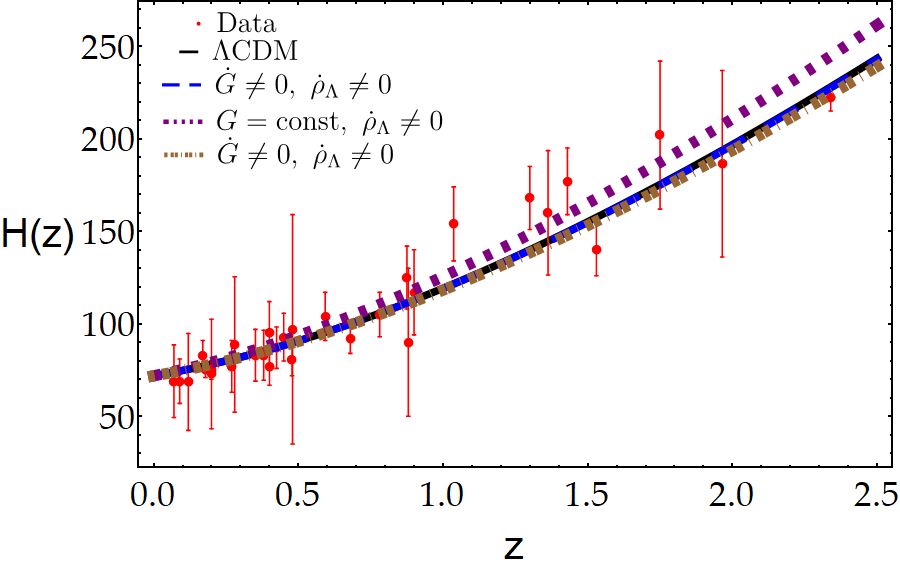
In Fig. (1) we show the comparison between experimental data (see text for details) and the computations under the CDM and the running–vacuum model previously discussed for . The values of the parameters were fixed as in Sola2016 . Given the experimental uncertainty, all the considered models reproduce fairly well the observations. Therefore, does not provide an stringent test and other observables are needed. At this point it is worth mentioning the recent work in Sola2017 , in which the authors constrain possible running–vacuum models using the cosmological observables SN Ia + BAO + + LSS + BBN + CMB. However, as we will show in the following section(s), is not enough to discriminate between CDM, running–vacuum and variational running–vacuum models.
As we have previously commented in the introduction, in the next section we will deduce the Einstein field equations assuming scale (temporal) dependent couplings for a FLRW background and we do a preliminary test of this variational running vacuum model (VRV hereafter) models by using as the fundamental observable. In order to do this, in the next section we will present the essentials of scale dependent gravity.
III Scale–dependent couplings and scale setting
In this section we will introduce the general scale–dependent framework. The notation follows closely Ref. Koch:2014joa as well as Refs. Koch:2016uso ; Rincon:2017ypd ; Rincon:2017goj ; Rincon:2017ayr ; Contreras:2017eza . The classical couplings are the Newton and the cosmological constant, both of them being promoted to scale–dependent couplings, namely, which, in general, depend on some coarse graining scale, such as the renormalization scale, . In addition, there are two independent fields, which are the metric and the scale field . The effective action is given by
| (12) |
In a top down approach one has to calculate the running couplings from an underlying model of quantum gravity such as it is for example done in Niedermaier:2006wt ; Reuter:2007rv ; Percacci:2007sz ; Litim:2008tt ; Reuter:2012id . First, implications of such a scale dependence have been studied in Bonanno:2000ep ; Bonanno:2006eu ; Reuter:2006rg ; Reuter:2010xb ; Falls:2012nd ; Cai:2010zh ; Becker:2012js ; Becker:2012jx ; Koch:2013owa ; Koch:2013rwa ; Ward:2006vw ; Burschil:2009va ; Falls:2010he ; Hindmarsh:2011hx ; Koch:2014cqa ; Bonanno:2016dyv ; Bonanno:2018gck ; Bonanno:2017gji . If one takes the concept of scale dependence seriously, physically feasible solutions of the effective quantum action (12) are obtained after choosing the arbitrary renormalization scale as a function of the physical variables describing the system e.g. . In particular for the case of cosmology this means that the scale should vary with time . Taking this into account while varying (12) with respect to one obtains the effective Einstein’s field equations Reuter:2003ca ; Koch:2010nn ; Domazet:2012tw ; Koch:2014joa ; Contreras:2016mdt
| (13) |
where the effective energy–momentum tensor is defined according to
| (14) |
and where is a tensor which takes into account the scale–dependence of the gravitational coupling. This term is given by the following expression
| (15) |
However, for a full and self-consistent variational treatment of (12) one needs to include also variations of the action with respect to
| (16) |
It is straight forward to show that only the combination of both, Eq. (16) and Eq. (13), guarantees the conservation of the stress–energy tensor Koch:2010nn ; Koch:2014joa . The use of equation (16) is typically quite involved such that an analytical treatment becomes seemingly impossible. For highly symmetric systems in the Einstein Hilbert truncation there is, however, a nice alternative to this procedure. For example in cosmology, symmetry dictates that the scale is only a function of time (). Since further the couplings are only functions of the scale (, ) one can conclude that the couplings are only functions of time (, ). Thus, one can avoid the source of non-analyticity in (16) by trying to solve only equation (13) directly for , and and replacing relation (16) by a well motivated ansatz (for example for ). Doing this, one can find explicit cosmological solutions, gain analytical understanding, and maintain the general covariance of the system.
Finally, it is worth mentioning that, in general, a solution for a scale–dependent model should recover the classical limit when certain running parameter is turned off Koch:2016uso ; Rincon:2017ypd ; Rincon:2017goj ; Rincon:2017ayr . However, as it will be shown later, this is not the case for certain VRV cases because the running parameter, which controls the strength of the scale dependence, can not be identified due to the numerical nature of the solutions (see Sects. III.3 and III.4 for details).
III.1 The model
Assuming again a flat universe (i.e. ) and considering dust matter (), the generalized Friedmann equations coming from (13) are
| (17) | ||||
| (18) |
The previous generalized Friedmann equations are the fundamental equations to be solved in all the cases considered in this section. Nevertheless, some of the cases that we will deal with will have more than two unknowns and therefore will require additional equations in order to solve for all the unknowns. In all such cases, we will either assume the covariant conservation of the energy momentum tensor or a perturbation ansatz for the baryonic energy density . We will justify the assumption of such additional information whenever we use it. In the rest of the work we will explore some particular cases of these VRV models, trying to constrain their validity by computing and comparing both with previous RV models and experimental data, as previously discussed. When possible, analytical solutions for will be given. For an appropriate comparison with RV models, the same cases are considered.
III.2 and
If , then and the VRV model is identical to the RV model previously discussed in subsection (II.2.1).
III.3 and
In this case, we assume the same ansatz for the baryonic energy density as we used in Section II.2.2, that is
| (19) |
in order to have enough information to solve the system. We use this ansatz in order to follow as close as possible the protocol usually implemented in RV models to solve the equations in each one of the cases. Even more, since we are introducing a parameter , we interpret it as a perturbation parameter with respect to the CDM model, therefore, its numerical value will be small. Taking into account the above, the system of differential equations to solve consist of just the generalized Friedmann equations, and in this particular case they are given by
| (20) | |||
| (21) |
After an appropriate manipulation of equations (20), (21) we get
| (22) |
It is worth mentioning that an analytical solution for the scale factor was not obtained due to the complexity of the equation.
III.4 and .
This is the most general case within the VRV framework. In addition to Friedmann equations, we assume the covariant conservations of the energy momentum tensor in order to have enough equations to solve for the unknowns and . We make this assumption since in this general case, we need to have the usual conservation of energy-momentum in order to properly compare the results of this case to the CDM model. Therefore, the corresponding equations in this case are
| (23) | ||||
| (24) | ||||
| (25) |
where, again, the first two equations correspond to the generalized Friedmann equations and the last one is the usual conservation of the energy momentum tensor. After manipulating the previous equations, introducing the dependences , considering the ansatz for given in Eq. (4), and doing the change of variables , we can solve numerically for the function .
III.5 Discussion
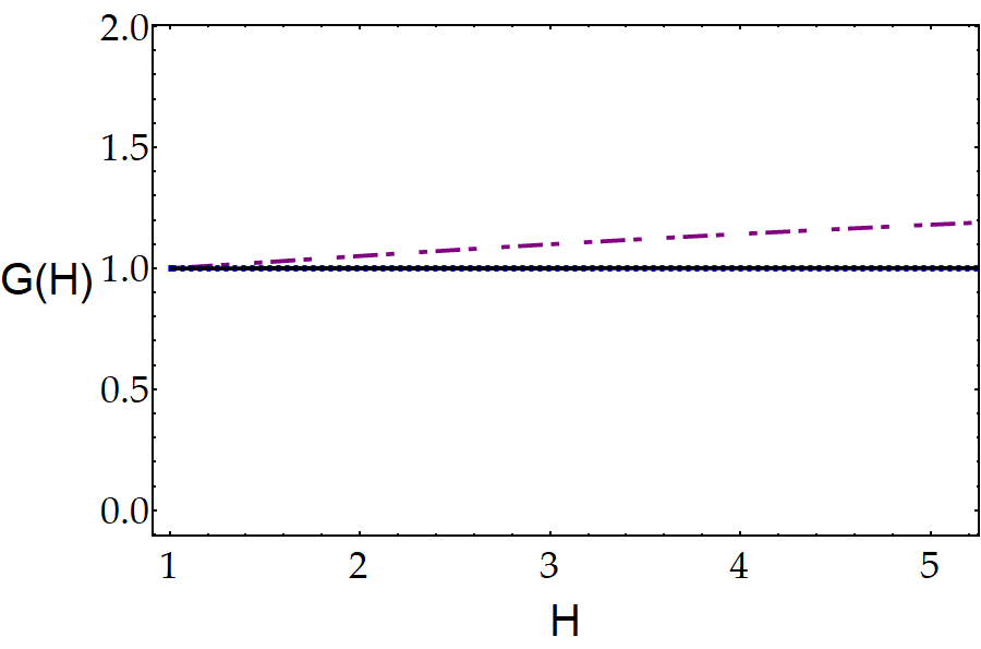
In Fig. (2) we show the comparison between the results of cases of subsections III.3 and III.4 with experimental data, showing that both of them fit well with the measurements. We note that this concordance with the expected behaviour could be due to a very slow decay of the Newton’s coupling in the context of a scale–dependent gravity, as shown in Fig. (3). To be more precise, the contribution of the Newton’s coupling encoded into is the way in which the energy-momentum tensor includes any possible deviation from the classical CDM model. Thus, given our solutions, the contribution of (see Eq. (15)) is expected to be small or at least the effect of a scale–dependent gravitational coupling on the classical solution is not dominant according to Fig. (3). Regarding the Fig. (3) we see that the RV case is essentially constant over this scale. We think that is the reason behind the nice fit between the RV predictions, the VRV predictions and experimental data. Nevertheless, a detailed study of this hypothesis is required in order to determine its validity.
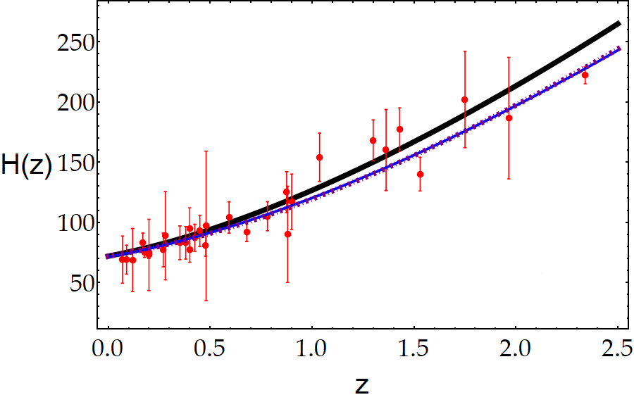
A more detailed comparison of the full running cases of both the RV model and the VRV model is shown in Fig. (4).
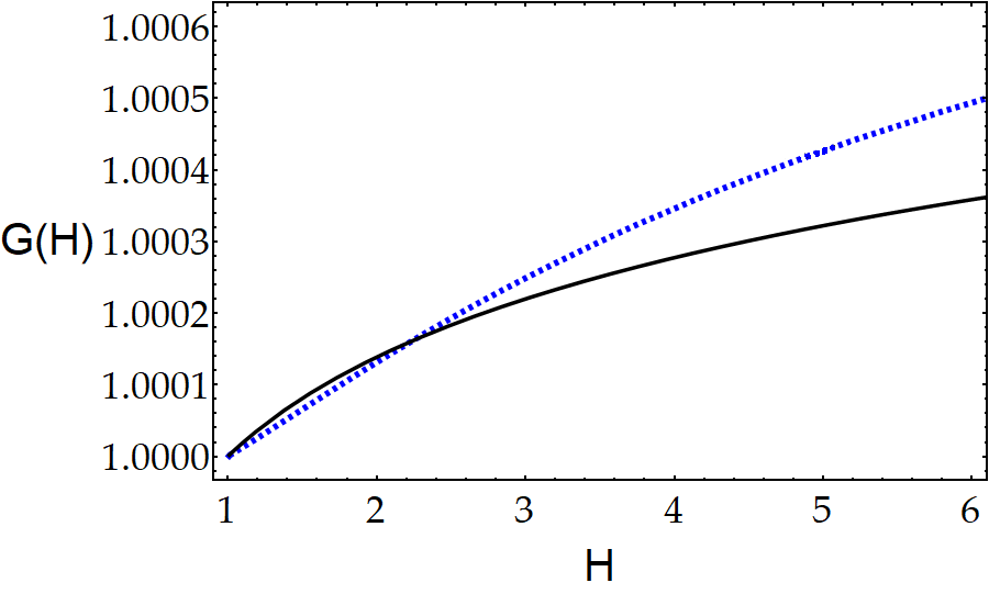
Let us remark that the VRV model here considered pass the preliminary test. We think that the main reason for this is the slow decay of with respect to the constant value of . In particular, deviations from the classical solution are related with the rate of change . Thus, in order to obtain a good agreement with the observational data, and should be small.
IV Concluding remarks
In this work we have introduced a scale–dependent cosmological model in a matter–dominated era. In the first part we have reviewed the so–called running vacuum models, incorporating some points not previously considered in the literature. In all these cases the model fits well with experimental data for by considering an standard equation of state for dark energy . Despite of that, it could be more satisfactory, for a theoretical point of view, to have a running vacuum model coming from a variational principle. In this spirit, starting with an effective action based on the usual Einstein–Hilbert one, we have promoted to scale–dependent couplings, to implement this scale–setting procedure into a cosmological context (variational running vacuum model) for a matter–dominated era in the second part. Specifically, and for the sake of comparison with other running vacuum models, we have limited our study to the case of time–dependent couplings. It is worth mentioning that we have also assumed the same ansatz for which were considered in the original running vacuum case. Note that, since this ansatz comes from QFT considerations in a FLRW background, we keep it as a suitable feature also for the variational running vacuum model. However, different parametrizations for coming from other approaches to quantum gravity could be assumed.
Within the variational procedure, we have studied several cases and a brief summary of the key points in each one of them is shown in Table 1.
| Case | Key point | Description |
|---|---|---|
| 1. | Classical GR, that is, CDM. | |
| 2. | and it is the same as RV case. | |
| 3. | and we assume . | |
| 4. | True running, in which we assume . |
First, if is taken as a constant value, an analytic solution for the modified Einstein’s field equations (including ) is obtained. It is worth mentioning that this solution does not correspond to a true running since the classical solution can not be recovered by turning off of any parameter. Therefore, once the running case has been considered, the classical case is automatically discarded. This feature is remarkable due in previous scale–dependent problems we always can recover the classical solution under certain choice of the so–called running parameter of the theory. Second, a complete numerical solution has been obtained when both and are taken into account into the model. Although this case corresponds to a true running, due to the numerics involved, we have not been able to find any parameter which could control the strength of the scale–dependence for both and . Third, regarding the comparison of these two models with the experimental data for , there are not significantly differences with respect to the CDM model. A possible explanation could be given in terms of the behaviour of the Newton’s coupling. As the classical solution implies a constant value, , for this coupling, we should expect the decay to be slow so that its variation, with respect to the classical case, is not appreciable. This turn out to be exactly the case, therefore the behaviour of the Newton’s coupling with respect to the constant coupling’s case could be an important point to take into account in order to test the viability of any extension of General Relativity, regardless of the fact that is not an observable of the model. In addition, we note that a slower decay of in the corresponding running vacuum case gives place to an excellent agreement with experimental data. Beyond that, it is necessary to say that what we did in this work is only a preliminary test to establish whether the scale dependent gravity theory fits well or not to the experimental data available for the time evolution of the Hubble factor, and although this preliminary test is satisfied by our variational running vacuum model, further test are required in order to decide if this model reproduces well the behaviour of our universe at all cosmological scales or not. Specifically, we can consider solar system test of our model or linear perturbations of both the metric and the energy densities. These and other aspects of scale–dependent cosmology are currently under study and will eventually be the object for future publication. To conclude, our model supports that the effective action of QFT in curved spacetimes can systematically incorporate quantum corrections through scale–dependent couplings. As far as we know, this is the first preliminary test that has been done about it.
V Acknowledgments
The author A. R. was supported by the CONICYT-PCHA/Doctorado Nacional/2015-21151658. The author B. K. was supported by the Fondecyt 1161150 and 1181694. The author P. B. was supported by the Faculty of Science of Universidad de los Andes, Bogotá, Colombia. The author A. H. A. was supported by the Faculty of Science of Universidad de los Andes, Bogotá, Colombia with the 2017-2 Call for Financiation of Research Projects for Master Students.
References
- (1) C. Patrignani et al., Chin. Phys. C 40, 100001 (2016).
- (2) P. A. R. Ade et al. Astron. Astrophys. 594, A13 (2016).
- (3) P. A. M. Dirac, Proc. Royal Soc. Lond. 365, 19 (1979) .
- (4) M. S. Berman and M. M. Son, Int. J. Theor. Phys 29, 1411 (1990).
- (5) O. Bertolami, Fortschritte der Physik 34, 829 (1986).
- (6) O. Bertolami, Nuov. Cim. B 93, 36 (1986).
- (7) M. S. Berman, Gen. Rel. Grav. 23, 465 (1991).
- (8) M. Reuter and H. Weyer, Phys. Rev. D 69, 104022 (2004).
- (9) B. Koch and I. Ramirez, Class. Quantum Grav. 28, 055008 (2011).
- (10) M. Reuter and H. Weyer, Phys. Rev. D 70, 124028 (2004).
- (11) D. Reeb, Subnucl. Ser. 46, 651 (2011).
- (12) B. Koch, I. A. Reyes and Á. Rincón, Class. Quantum Grav. 33, 225010 (2016).
- (13) Á. Rincón, B. Koch and I. Reyes, J. Phys. Conf. Ser. 831, 012007 (2017).
- (14) Á. Rincón, E. Contreras, P. Bargueño, B. Koch, G. Panotopoulos and A. Hernández-Arboleda, Eur. Phys. J. C 77, 494 (2017).
- (15) Á. Rincón and B. Koch, arXiv:1705.02729.
- (16) E. Contreras, Á. Rincón, B. Koch and P. Bargueño, Int. J. Mod. Phys. D 27, 1850032 (2018).
- (17) Á. Rincón and G. Panotopoulos, Phys. Rev. D 97, 024027 (2018).
- (18) E. Contreras, Á. Rincón, B. Koch and P. Bargueño, Eur. Phys. J. C 78, 246 (2018).
- (19) Á. Rincón and B. Koch, arXiv:1806.03024.
- (20) E. Contreras and P. Bargueño, Int. J. Mod. Phys. D 27, 1850101 (2018).
- (21) J. D. Barrow, Mon. Notices Royal Astron. Soc 282, 1397 (1996).
- (22) J. D. Anderson, G. Schubert, V. Trimble and M. R. Feldman, EPL 110, 10002 (2015).
- (23) H. Fritzsch and J. Solà, Mod. Phys. Lett. A 30, 1540034 (2015).
- (24) H. Fritzsch, R. C. Nunes and J. Solà, Eur. Phys. J. C 77, 193 (2017).
- (25) S. Desai, EPL 115, 20006 (2016).
- (26) J, Solà, A. Gómez–Valent and J. de la Cruz–Pérez, Astrophys J. 836, 43 (2017).
- (27) J. Solà and A. Gómez–Valent, Int. J. Phys. D 24, 1541003 (2015).
- (28) S. Weinberg, Cosmology, Oxford University Press (2008).
- (29) I. Shapiro, J. Solà, C. España–Bonet and P. Ruiz–Lapuente, Phys. Lett. B 574, 149 (2003).
- (30) C. España–Bonet, P. Ruiz–Lapuente, I. L. Shapiro and J. Solà, J. Cosmol. Astropart. Phys. 02, 6 (2004).
- (31) J. Solà and A. Gómez–Valent, MNRAS 448, 2810 (2015).
- (32) B. Guberina, R. Horvat and H. Nikolić, Phys. Lett. B 636, 80 (2006).
- (33) J. Solà, AIP Conf. Proc 1606, 19 (2014).
- (34) B. Koch, P. Rioseco and C. Contreras, Phys. Rev. D 91, 025009 (2015).
- (35) M. Niedermaier and M. Reuter, Living Rev. Rel. 9, 5 (2006).
- (36) M. Reuter and F. Saueressig, in Geometric and Topological Methods for Quantum Field Theory, H. Ocampo, S. Paycha and A. Vargas (Eds.), Cambridge Univ. Press, Cambridge (2010).
- (37) R. Percacci, in Approaches to Quantum Gravity: Towards a New Understanding of Space, Time and Matter, D. Oriti (Ed.), Cambridge Univ. Press, Cambridge (2009).
- (38) D. F. Litim, PoS(QG-Ph) 024 (2008).
- (39) M. Reuter and F. Saueressig, New J. Phys. 14, 055022 (2012).
- (40) A. Bonanno and M. Reuter, Phys. Rev. D 62, 043008 (2000).
- (41) A. Bonanno and M. Reuter, Phys. Rev. D 73, 083005 (2006).
- (42) M. Reuter and E. Tuiran, arXiv: 0612037
- (43) M. Reuter and E. Tuiran, Phys. Rev. D 83, 044041 (2011).
- (44) K. Falls and D. F. Litim, Phys. Rev. D 89, 084002 (2014).
- (45) Y. F. Cai and D. A. Easson, JCAP 1009, 002 (2010).
- (46) D. Becker and M. Reuter, JHEP 1207, 172 (2012).
- (47) D. Becker and M. Reuter, arXiv:1212.4274.
- (48) B. Koch and F. Saueressig, Class. Quantum Grav. 31, 015006 (2014).
- (49) B. Koch, C. Contreras, P. Rioseco and F. Saueressig, Springer Proc. Phys. 170, 263 (2016).
- (50) B. F. L. Ward, Acta Phys. Polon. B 37, 1967 (2006).
- (51) T. Burschil and B. Koch, Zh. Eksp. Teor. Fiz. 92, 219 (2010).
- (52) K. Falls, D. F. Litim and A. Raghuraman, Int. J. Mod. Phys. A 27, 1250019 (2012).
- (53) M. Hindmarsh, D. Litim and C. Rahmede, JCAP 1107, 019 (2011).
- (54) B. Koch and F. Saueressig, Int. J. Mod. Phys. A 29, 1430011 (2014).
- (55) A. Bonanno, B. Koch and A. Platania, arXiv:1610.05299.
- (56) A. Bonanno, A. Platania and F. Saueressig, arXiv:1803.02355.
- (57) A. Bonanno, S. J. Gabriele Gionti and A. Platania, Class. Quantum Grav. 35, 065004 (2018).
- (58) M. Reuter and H. Weyer, Phys. Rev. D 69, 104022 (2004).
- (59) B. Koch and I. Ramirez, Class. Quantum Grav. 28, 055008 (2011).
- (60) C. Contreras, B. Koch and P. Rioseco, Class. Quantum Grav. 30, 175009 (2013).
- (61) B. Koch and P. Rioseco, Class. Quantum Grav. 33, 035002 (2016).
- (62) S. Domazet and H. Stefancic, Class. Quantum Grav. 29, 235005 (2012).
- (63) B. Koch, P. Rioseco and C. Contreras, Phys. Rev. D 91, 025009 (2015).
- (64) C. Contreras, B. Koch and P. Rioseco, J. Phys. Conf. Ser. 720, 012020 (2016).
- (65) J. Grande, J. Solà, J. Fabris and I. Shapiro, Class. Quantum Grav. 27 , 105004 (2010).
- (66) J. Solà, Int. J. Mod. Phys. A. 31, 1630035 (2016).
- (67) J. Fabris, B. Chauvineau, D. Rodrigues, C. Almeida and O. Piattella, arXiv:1603.01314.
- (68) S. Nojiri, S. Odintsov and V. Oikonomou, Phys. Rep. 692, 1 (2017).
- (69) G.B Zhao, et. al., Nat. Astron. 1, 627 (2017).
- (70) J. Solà, A. Gómez-Valent and J. de Cruz Pérez, Phys. Lett. B 774, 317 (2017).