Single-Volume Neutron Scatter Camera for High-Efficiency Neutron Imaging and Spectroscopy

Abstract

Neutron detection provides an effective method to detect, locate, and characterize sources of interest to nuclear security applications. Current neutron imaging systems based on double-scatter kinematic reconstruction provide good signal vs. background discrimination and spectral capability, but suffer from poor sensitivity due to geometrical constraints. This weakness can be overcome if both neutron-proton scattering interactions are detected and resolved within one large contiguous active detector volume. We describe here a maximum likelihood approach to event reconstruction in a single-volume system with no optical segmentation and sensitivity to individual optical photons on the surfaces of the scintillator. We present results from a Geant4-based simulation establishing the feasibility of this single-volume neutron scatter camera concept given notional performance of existing photodetector and readout technologies.

1 Introduction

Fission-energy neutrons are a sensitive and specific signature of special nuclear material, due to their low and stable natural backgrounds, their penetrating nature, and the scarcity of benign neutron-emitting materials. As such, neutron imaging has the potential to be an important tool in a range of nuclear security applications, including arms control treaty verification, emergency response, cargo screening, and standoff search. In particular, neutron scatter cameras (NSC) have become an established technology for fission-energy neutron imaging and spectroscopy [1, 2, 3, 4, 5]. Based on the kinematic reconstruction of neutron double scatters, NSC systems provide excellent event-by-event directional information for signal-to-background discrimination, reasonable imaging resolution, and good energy resolution when compared to competing imaging technologies [5, 6, 7, 8].

The operational principle of an NSC is based on the neutron elastically scattering on hydrogen at least twice in the detector’s active material, typically an organic scintillator. The incoming kinetic energy $E_{\text{n}}$ is obtained from

$$E_{\text{n}}=E_{\text{n}^{\prime}}+E_{\text{p}}$$ (1)

as the sum of the energy $E_{\text{p}}$ deposited in the first scatter, which is assumed to generate a recoiling proton, plus the scattered neutron energy $E_{\text{n}^{\prime}}$. This in turn is calculated from

$$E_{\text{n}^{\prime}}=\frac{1}{2}m_{\text{n}}\left(\frac{d_{10}}{t_{10}}\right)^{2},$$ (2)

using the measured distance $d_{10}$ and time $t_{10}$ between the first two scatters. These quantities also allow for a calculation of the scattering angle $\theta$ defining a cone containing the incoming neutron direction:

$$\theta=\arccos\left(\sqrt{\frac{E_{\text{n}^{\prime}}}{E_{\text{n}}}}\right).$$ (3)

Most existing NSC systems consist of arrays of spatially-separated organic scintillator cells in order to isolate in two distinct cells the neutron’s two elastic scatters [1, 2, 3, 4, 5]. This requirement, however, has poor geometrical efficiency, constituting the primary drawback of current NSC systems.

The design concept of a single-volume neutron scatter camera (SVSC), in which both neutron scatters occur in the same large active volume, addresses this drawback. Given that the interaction length of fission-energy neutrons in organic materials is a few cm, the detector’s principle relies on the ability to resolve two proton recoils in a contiguous scintillator volume at spatial and temporal separations of order $1~{}\text{cm}$ and $1~{}\text{ns}$ respectively. This reconstruction of the neutron interaction locations must be based on the arrival time and position of the scintillation photons at the boundaries of the active volume. While traditional photomultiplier tubes (PMTs) cannot provide the necessary spatial and temporal resolution, recent advances in photodetector (PD) technology have made the approach possible [9]. Photodetectors based on micro-channel plate (MCP) electron multipliers [10] inherently provide the spatial and temporal photon detection resolution that makes them attractive for single-volume event reconstruction. These MCP-PMTs have found application in a wide variety of areas ranging from medical imaging [11] to neutrino detection [12, 13]. Commercially available photodetectors have $2-6~{}\text{mm}$ two-dimensional pixels and sub-ns timing [14], while models under development will potentially provide large area photocathode coverage at relatively low cost [15]. In this work, we investigate the feasibility of the SVSC concept using Monte Carlo simulation studies of a system with PD performance motivated by available MCP-PMTs.

Throughout this paper, the term “single-volume” means that the active detection volume is compact and essentially contiguous, rather than spread out spatially in discrete well separated volumes (cells, planes, etc.). We refer to an individual neutron scatter, most usefully neutron-proton elastic scattering, as an “interaction”, and to a neutron history, which may include multiple interactions, as an “event”. In an experimental context, an event can mean the data collected by a single trigger, which could include information from zero (noise), one, or more (pileup) particles. “Event reconstruction” is an algorithm that uses the observable optical photon information to determine the locations and times of neutron interactions in the event. Many such reconstructed events can then be combined to reconstruct a neutron image and energy spectrum.

This article is structured as follows. We begin in Sec. 2 with the general motivation and design-agnostic arguments for a single-volume neutron scatter camera, as well as a survey of several possible design classes. In Sec. 3, we describe the “direct reconstruction” SVSC concept as simulated in this paper, emphasizing how the design choices are enabled by existing technology. The data processing and reconstruction steps required by this concept are also detailed in Sec. 3. The rest of the paper is dedicated to a demonstration of the feasibility of the SVSC concept based on Monte Carlo simulation data. Details of the simulated model and the corresponding physical behavior of the system directly obtained from the simulation are presented in Sec. 4. The results of the data processing stage applied to the simulated data, which will cover the event reconstruction and the source spectral and image reconstruction, are presented in Sec. 5 together with an analysis of the instrument’s limitations.

2 General considerations for a single-volume neutron camera

We begin with a discussion of the motivation for and approaches to single- volume neutron imaging, without reference to a specific concrete detector system design.

2.1 Advantages of single-volume neutron imagers

The motivation for research into a single-volume double-scatter neutron imager rests on the potential for significant improvements over cell-based scatter camera designs in two important aspects: imaging efficiency and compactness.

A single-volume camera addresses two of the important efficiency limitations of the NSC: the requirement of no more than one neutron scatter in the first detector element (in order for a one-to-one relationship between fractional energy deposited and scattering angle to be valid), and the geometrical efficiency for the scattered neutron to pass through a second detector element. Assuming the ability to resolve scattering events at $2~{}\text{cm}$ separation in the single volume, an estimate of the improvement in efficiency for double-scatter neutron detection, relative to the NSC of [7], is about an order of magnitude.

To obtain this estimate, an MCNP [16] simulation was performed: a fission neutron pencil beam was fired at the center of one of the middle detectors in the conventional NSC front plane, and at the center of a $20~{}\text{cm}\times 20~{}\text{cm}\times 20~{}\text{cm}$ volume of scintillator. The NSC was simulated with a standard plane separation of $40~{}\text{cm}$. The fraction of events satisfying simple requirements were tallied: first, that two interactions occur—as a function of the distance between the first two neutron scatter interactions for the single-volume system, and with a front and rear plane requirement for the current NSC; second, that both interactions were hydrogen scatters (carbon recoils are typically too quenched to observe); and third, that both interactions deposited at least $200~{}\text{keV}$, an optimistic threshold. In Fig. 1, the results are shown for the single-volume system as a function of the distance between the first two interactions. The corresponding fractions for the cell-based NSC are 0.026 for the first two interactions in the front and rear planes; 0.013 for both scatters producing proton recoils; and 0.008 for both protons having at least $200~{}\text{keV}$. The SVSC yields a significant improvement over the conventional NSC in potential efficiency when the minimum separation between interactions is low. For a $2~{}\text{cm}$ minimum interaction spacing, the number of potentially detectable events is slightly over an order of magnitude higher in the SVSC than in the current NSC. Even at $10~{}\text{cm}$ minimum interaction spacing, the fraction of usable neutrons is comparable to the current NSC. Further study will be needed to understand the relative power of events with small separation in a SVSC, since the energy and imaging resolutions will degrade with smaller separation distances.

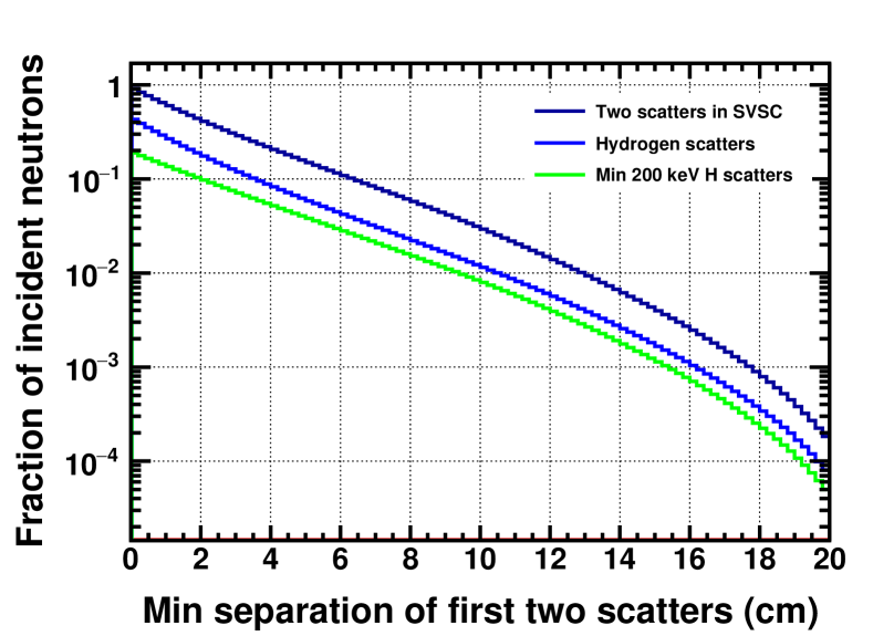
Figure 1: Potential efficiency for the proposed single-volume scatter camera. Details of the MCNP simulation are given in the text. No experimental resolution effect or detection efficiency is included, beyond the requirements listed. The values are given as a function of the distance separating the first two interactions in the volume; the ability to distinguish interactions at smaller separations increases the potential efficiency of the detector.

Additionally, the overall detector footprint is more compact and lighter: about $40~{}\text{cm}\times 40~{}\text{cm}\times 20~{}\text{cm}$, with expected weight about $10-20~{}\text{kg}$ for the same scintillator volume as the 32-element SNL NSC, which takes up a volume of approximately $1~{}\mathrm{m}^{3}$ and weighs more than $200~{}\text{kg}$. Easier transport and deployment is a key benefit for some applications. Moreover, a more compact detector allows to get closer to the source, which in turn increases detection rate according to the inverse square of the distance to the source, and improves spatial resolution at the object for a given angular resolution.

2.1.1 Four single-volume imager concepts

Single-volume neutron imaging is predicated on the ability to use the information encoded in the optical photons emitted by the scintillator to reconstruct the scattering history of the neutron in the active volume. Even if it is granted that from an information theory perspective there is in fact sufficient information retained by the optical photons to do this, it is still one of the key technical challenges of this research to develop detector designs and algorithms that accurately (and tractably) do it. Four general methods that have been considered for building a single-volume neutron imager are as follows.

Direct reconstruction

This method is conceptually the simplest and yet technically the most challenging. The scintillator is a single monolithic volume, and optical photons are detected at the boundaries of the volume. The neutron interactions are reconstructed based on the information in the detected photon positions and times, accounting for the isotropic photon emission from the scintillator, the scintillator pulse shape, photon speed and attenuation in the scintillator, photodetector efficiency, etc. This paper documents studies of this concept.

Optical segmentation

The “single volume” of scintillator is formed from multiple pillars of scintillator, separated by reflective boundary layers. The goal is to trap the optical photons from an interaction in one pillar, reading them out from both ends. For each interaction, the location along the long dimension of the pillar is determined by the amplitude ratio and/or time difference of the light observed at each end, while the transverse location is determined by which pillar the light is observed in. When two interactions occur in different pillars, their locations and times can be independently determined, constituting an event reconstruction. Simulation studies toward a realization of this concept are detailed in [8].

Optical coded aperture

This method, like direct reconstruction, uses a single uninterrupted scintillator volume, but instead of directly detecting and reading out the optical photons on the boundary of the volume, they pass through a coded aperture on each side. This has the advantage of introducing a high-frequency spatial component to the detected photon distribution, which eases the spatial reconstruction of interaction locations. Disadvantages include the loss of a significant fraction (typically 50%) of the photons to the mask, and the presence of light guide material, which is necessary to allow the photons to spread before and after the coded mask, but also results in an inactive scattering/attenuating layer that neutrons must penetrate before reaching the active volume. A similar approach has been studied for gamma Compton imaging [17].

Optical lattice

This is similar to the optical segmentation approach, but aims to create virtual “pillars” in all three dimensions. Small cubes of scintillator are separated by very thin air gaps in a three-dimensional array. The scintillator-air boundaries create total internal reflection (TIR) for photons hitting them at larger than the critical angle. Some photons experience TIR in each of the three dimensions of the lattice, and are therefore confined to a single “pillar” or row of cubes. Light therefore arrives as a bright spot on all six sides of the array, not just two. This approach has been studied for neutrino detection [18].

It should be noted that the reconstruction uncertainties, and consequently the directional and spectral resolving power, of each event in single-volume designs depend significantly on the design details, component performance (scintillator time profile, photodetector efficiency and resolution, etc.), and reconstruction algorithms used. On the one hand, a single-volume design will be able to determine the location and time of neutron interactions with better resolution than the NSC. On the other hand, we expect reduced precision in the measurements of deposited energy when disentangling the light output from multiple interactions, and the short lever arm between the two neutron interactions also decreases imaging resolution with respect to the cell-based design. In the remainder of this paper, we focus on further exploring the direct reconstruction technique.

3 Single-volume scatter camera design

We now proceed to specify a concrete detector system design and reconstruction algorithm for full simulation studies of a single-volume imager.

3.1 SVSC system as simulated

The direct reconstruction SVSC design concept, schematically shown in Fig. 2, consists of an organic scintillator volume with each side optically coupled to and fully covered by fast-timing high-gain MCP-PMTs. These photodetectors play the central role of registering the arrival time and position of the isotropically emitted photons produced by particle interactions in the scintillator volume. As already mentioned, current MCP-PMT technology, either available or under development, can provide photon timing resolution on the order of $100~{}\text{ps}$ and mm-scale spatial photon detection resolution. The simulation studies presented in Sec. 4 show the impact on the event reconstruction due to such finite MCP-PMT resolution values by comparing results with idealized photodetectors able to provide exact time and spatial photon coordinates, and demonstrate the detector’s spectral and image reconstruction capabilities even with existing MCP-PMT technology. Another enabling consideration of the SVSC concept is ability of high speed waveform sampling required to take advantage of the intrinsic time resolution of MCP-PMTs, and especially to disentangle multiple photons arriving in one photodetector pixel within a timescale of nanoseconds. This is possible using switched capacitor array sampling, such as with the Domino Ring Sampler chips, which provide up to $5~{}\text{GS/s}$ sampling frequency [19, 20, 21]

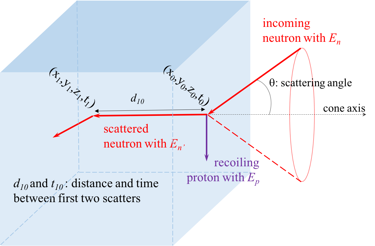
Figure 2: Sketch of a neutron event in the SVSC. The neutron interacts twice in the SVSC scintillator volume. If the position and time of the two interactions can be reconstructed using the optical photons emitted in the scintillator, then the incoming neutron energy and direction (up to a conical ambiguity) can be determined through the kinematic properties of neutron-proton elastic scattering.

When selecting the active material type, fast scintillation decay time represents the main driver, even more important than the ability to discriminate neutrons and gammas via pulse shape discrimination (PSD). Narrow scintillation pulses allow for better event timing reconstruction, especially when reconstructing events with several neutron interactions. Although PSD is desirable for this system, it may be superfluous since we already require the ability to reconstruct the time of flight of the detected particle, which provides neutron/gamma discrimination. High light output is also desired, as photon statistics is one limiting factor in the event reconstruction described below, although we note that the readout and signal processing are simplified if the photon occupancy per MCP-PMT pixel is low. Here we simulate EJ-232Q  [22], a quenched plastic scintillator with pulse width of less than $400~{}\text{ps}$ but only 19% anthracene light output, a choice that emphasizes the pulse width over photostatistics. The scintillator size is set to a $10~{}\text{cm}$ cube in order to guarantee a high probability of double neutron scatters, in accordance with the interaction length for fission-energy neutrons. In general, the choice of active volume size will be dictated by a variety of factors, like detection rate and efficiency requirements, hardware constraints and application-specific trade-offs, which go beyond the scope of this paper.

3.2 Reconstruction algorithms

Data processing and analysis are essential elements in the design and operation of the SVSC. They are accomplished in three separable analysis stages: single-photon isolation in each individual pixel, neutron double-scatter event reconstruction, and the final image and spectrum reconstruction.

Single-photon isolation is the process of assigning an arrival time and location to each detected photon using the digitized raw traces from each MCP-PMT channel (or pixel). The specifics of this part of the analysis are highly coupled to the experimental behavior of the photodetector and electronics. For this simulation study, since the goal is to determine feasibility of the concept, we make the optimistic assumption that all detected photons can be individually identified.

For event reconstruction, we employ the direct reconstruction of particle interactions using the arrival position and time of isotropically emitted photons at the scintillator surface. Multiple methods have been explored; here we use the unbinned maximum likelihood (ML) technique. The likelihood function is maximized for a given event when the fixed set of observations (the list of detected photon coordinates and times) has the highest probability of occurring as the event parameters (the list of neutron interaction locations and times) are varied. Put another way, the ML algorithm finds the neutron trajectory that would be most likely to produce the observed data. We use the extended maximum likelihood [23],

$$\mathcal{L}=\frac{\mathrm{e}^{-\mu}\mu^{n}}{n!}\prod_{i=1}^{n}\sum_{j=1}^{N}\frac{\mu_{j}}{\mu}P_{j}(\vec{x_{i}}),$$ (4)

where $\mu_{j}$ is the number of photons detected from neutron interaction $j$ and $\mu=\sum\mu_{j}$, $n$ is the number of detected photons, $N$ is the number of neutron interactions assumed, $\vec{x_{i}}$ represents the detected position and time of photon $i$, and $P_{j}(\vec{x_{i}})$ is the probability to observe photon $i$ from interaction $j$. Each photon could have come from any of the neutron interactions, so the probability to observe each photon is summed across interactions; each photon is an independent observation, so the photon probabilities multiply. Looking more closely at the probability function, we have

$$P_{j}(\vec{x_{i}})=\frac{\cos\phi_{ij}}{4\mathrm{\pi}d_{ij}^{2}}\cdot\mathrm{e}^{\frac{-d_{ij}}{\lambda}}\cdot f(t_{i}-t_{j}-d_{ij}/c_{p}).$$ (5)

The first term accounts for solid angle between the location of emission (interaction $j$) and the location of detection for photon $i$. The angle between the line connecting the two locations and the normal of the photodetector surface is $\cos\phi_{ij}$, and $d_{ij}$ is the distance between the two locations. The second term accounts for attenuation in the scintillator material, where $\lambda$ is the attenuation length. In the third term, $f(t)$ is the pulse shape of the scintillator, where the time difference between the photon emission and detection has been corrected for the flight time of the photon ($c_{p}$ is the speed of light in the medium). The likelihood maximization itself is performed using the SIMPLEX and MIGRAD algorithms as implemented by the MINUIT package in the ROOT software [24].

This likelihood maximization results in an estimate of the position, time, and intensity of each neutron interaction, and an associated variance-covariance matrix (via inverting the Hessian matrix at the log-likelihood maximum). From these fitted quantities, we then derive $d_{10}$, $t_{10}$, and the cone axis direction, as shown in Fig. 2, and their uncertainties. Finally, the kinematic equations Eqs. 1–3 are used to determine the ultimate quantities of interest, namely $E_{\text{n}}$ and the cone opening angle $\theta$. In all cases, the fit errors are propagated to the derived results via the standard linearized approximation, including correlations.

Finally, image reconstruction is performed from many such neutron events using a Maximum Likelihood Estimation Maximization (MLEM) algorithm  [25]. We use a list-mode implementation of MLEM, in which a simplistic system response is calculated for each observed event, under the assumption that the reconstructed cone axis and opening angle are accurate within uncertainties.

4 Simulation

A Monte Carlo model of the SVSC detector system was constructed using Geant v4.10.01.p02 [26]. The scintillator material as described in Sec. 3.1 is centered at the coordinate origin. A $1~{}\text{mm}$ thick acrylic light guide representing an optical coupling encloses the scintillator, which is then completely surrounded by a $1~{}\text{mm}$ quartz layer of very short optical absorption length representing the MCP-PMT. An isotropic point-like ${}^{252}\text{Cf}$ neutron source is placed at $1~{}\text{m}$ from the origin along the $y$ axis.

The simulation uses the physical attributes listed in Table 1. Neutron interactions are modeled by the Geant4 NeutronHP cross-section package, which includes high precision hadronic models for energies below $20~{}\text{MeV}$, appropriate for fission-energy neutrons. Scintillation photons from electron recoils are generated according to the manufacturer-reported scintillation efficiency for EJ-232Q with 0.5% benzophenone concentration. Due to lack of experimental data on proton quenching in this scintillator, we use the energy-dependent proton light output measured for a similar plastic scintillator in [27], and we model the carbon recoil light output according to [28]. The photon generation time profile follows the manufacturer-reported exponential rise and decays times, shown in Table 1, with a reported scintillation pulse width of $360~{}\text{ps}$. The optical interfaces between the scintillator, the light guide and the photodetector are assumed to be perfectly smooth, and photons are either reflected or transmitted but are not absorbed in the materials interface. A wavelength-dependent refraction index is used for the acrylic light guide [29]. Optical photon detections per event are recorded over a $100~{}\text{ns}$ window. In order to account for the photocathode quantum efficiency, photons absorbed in the photodetector volume are randomly saved with 25% efficiency.

Table 1: Numerical values of various parameters used in the GEANT4 simulation of the SVSC concept. Component abbreviations: SC refers to the scintillator; LG refers to the light guide; PD refers to the photodetector.

Attribute	Value
SC cube size	$100~{}\text{mm}$
SC Efficiency	$2900~{}\text{ph/MeVee}$
SC pulse rise time	$0.11~{}\text{ns}$
SC pulse decay time	$0.7~{}\text{ns}$
SC absorption length	$8~{}\text{cm}$
SC refraction index	1.58
LG refraction index	1.49–1.59
PD quantum efficiency	0.25
PD absorption length	$10^{-3}~{}\text{mm}$
PD refraction index	1.57
PD time spread	$0.1~{}\text{ns}$
PD pixel size	$5.9~{}\text{mm}$

The left plot of Fig. 3 shows the histograms of the number of neutron elastic collisions within the scintillator volume, normalized by the number of primary neutrons that interact in the detector. When a $300~{}\text{keV}$ threshold is imposed on the neutron deposited energy—which corresponds to about $40~{}\text{keVee}$ of proton light output in EJ-232Q or, equivalently, to only about 30 detected photons—the number of above-threshold neutron collisions per event is reduced drastically. This indicates that the transfer of most of the neutron’s energy to the scintillator is usually done in few elastic scatters.

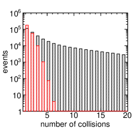
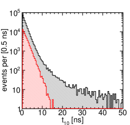
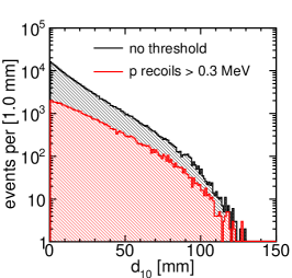
Figure 3: Truth-level results from the GEANT4 simulation of a ${}^{252}\text{Cf}$ source. Left: The number of neutron elastic collisions. Middle: The time difference between the first two neutron interactions, for neutrons interacting at least twice in the scintillator. Right: The distance between the first two neutron interactions, for neutrons interacting at least twice in the scintillator. No threshold on the deposited energy was imposed on the neutron interactions populating the histograms in black, while the histograms in red only include interactions creating proton recoils that deposit more than $300~{}\text{keV}$. Moreover, only events where the first two proton recoils are above the threshold are included in the $t_{10}$ and $d_{10}$ red histograms.

The middle and right histograms of Figure 3 show the histograms of the time and distance between the first two neutron collisions. These quantities, along with the energy transferred in the first collision, contain the information from which the neutron’s incoming energy and direction can be extracted. For zero threshold, the mean distance between the first two neutron collisions is about $1.8~{}\text{cm}$, increasing to $2.4~{}\text{cm}$ for collisions above $300~{}\text{keV}$, and the mean time remains $\sim 1.7~{}\text{ns}$ in both threshold cases.

The arrival time and spatial coordinates of the individual optical photons from all neutron collisions, regardless of deposited energy, constitute the input data for the event reconstruction algorithm described above. In order to include the effect of finite timing resolution in the MCP-PMT and electronics, the photon arrival time was Gaussian smeared with standard deviation equal to $0.1~{}\text{ns}$, which is informed by the transit time spread in existing detectors and bandwidth of available electronics [14, 30]. The photon two-dimensional coordinates along each photodetector plane—e.g., the $(x,y)$ coordinates of the photodetector at $z=50~{}\text{mm}$—were also Gaussian smeared. For the coordinates smearing, we use a standard deviation equal to $(5.9~{}\text{mm})/\sqrt{12}=1.7~{}\text{mm}$, which matches the standard deviation of a rectangular distribution with width $5.9~{}\text{mm}$ representing the pixel size of the Planacon XP85012.

In the following two ways, the current study takes advantage of information that is known in simulated events but not in real data, and therefore potentially over-estimates the system performance. First, we constrain the total number of neutron collisions, $N$, to be the simulated number of neutron scatters depositing more than $300~{}\text{keV}$. In real data, it should be possible to estimate the number of energetic collisions in the scintillator volume from the spatially integrated photon detection time profile combined with the time-sliced spatial distributions of photon detection locations. We note that there is no obviously “correct” value for $N$: counting real but low-energy collisions into $N$ adds irrelevant degrees of freedom to the MINUIT minimization, increasing the probability of incorrect convergence of Eq. (4). A process of iterative minimizations with $N$ ranging over most likely values according to the observed signals could be part of the event reconstruction algorithm when working with real data.

Second, in this study, small deviations from the interactions’ actual location coordinates ($0.5~{}\text{mm}$), time ($0.1~{}\text{ns}$), and number of emitted photons (50) are used to set the initial guesses in the minimization algorithm. (Events for which the minimization algorithm does not move from these initial parameter values are rejected as failed fits.) In the limit of a globally convex likelihood function, this procedure does not produce a bias, as the fit will converge to the same global minimum regardless of the initial position. However, in the case that the function has multiple local minima, this procedure could bias the results by over-estimating the accuracy of the initial guess that could be achieved. Again, in real data, initial guesses could be extracted from rough analysis of the photon detections, but we leave the development and demonstration of such an algorithm to future work.

Idealizations in our simulated model could play a more relevant role in the reconstruction algorithm success. Complete wavelength dependence of optical processes is not included. The optical interfaces between the scintillator, the light guide and the photocathode are assumed to be perfectly polished surfaces with nearly matching indexes of refraction, and thus, most simulated photons are transmitted and absorbed in the photocathode. However, a realistic detector will likely suffer from increased photon scattering in the optical surfaces due to imperfect optical coupling and surface roughness. Any scattered photons that are later detected by the photodetectors will not satisfy the reconstruction’s assumption of being directly emitted from interaction locations, and thus, will affect the event reconstruction success. Additionally, the detected photon count of a real detector is expected to be smaller than that of our simulated model due to incomplete photocathode coverage and other unmodeled optical absorption effects. Furthermore, we assume in simulation that each photon can be individually resolved and accurate arrival time can be assigned, but the overlapping of their corresponding single-photoelectron waveforms, already discussed in Sec. 3, will affect the photon count and timing per photodetector pixel. Finally, here we simulate and reconstruct only neutron events. In reality, some gamma interactions will be misidentified as neutrons and contribute erroneously to a neutron image.

Due to the assumptions and limitations of the simulation model described above, the event reconstruction and the image reconstruction results presented in the next section should be understood as an upper limit on the performance of the SVSC detector concept. Put another way, we aim here to establish feasibility of the SVSC design, rather than to accurately predict performance of a system.

5 Simulation results

In order to quantify the event reconstruction performance, we define the “true” variables in a given event as the positions, times, and intensities of the first two n-p scatters in the simulation, as well as the higher-level quantities (e.g. $d_{10}$ or $\theta$) calculated from those. Note that in some classes of events, such as those with an initial carbon scatter before two hydrogen scatters, the “true” reconstructed cone may not include the incident direction since the kinematic assumptions are not valid. But the goal of the event reconstruction is to determine the attributes of the proton recoils, so we evaluate it on that basis.

For each variable, we construct resolution plots, i.e. histograms of the difference between the reconstructed and the true variables; these are plotted in Figs. 4–7 and will be discussed below in turn. The differences are denoted with the symbol $\Delta$ followed by the variable symbols defined in Fig. 2. In these plots, the photon arrival time $T$ and coordinates $(X,Y,Z)$ that entered the reconstruction algorithms have been smeared as described in the previous section, and only events for which the likelihood maximization converged are included. Each histogram is plotted with a fitted Gaussian function, whose mean ($\mu$) and width ($\sigma$) are given in the plot as well as in Table 2.

Table 2: The event reconstruction resolutions are summarized in this table. The mean $\mu$ and width $\sigma$ of Gaussian fits to the various reconstructed quantities are given; this represents the bias and resolution of the reconstruction for this simulated system and ${}^{252}\text{Cf}$ source. Refer to Fig. 2 for definitions of the variables. Results are presented for reconstructions using both smeared (representing experimental resolutions) and the exact (as obtained from the simulation) photon positions and times. See text for discussion of the $\Delta\alpha$ distribution.

	Smeared		Exact
	$\mu$	$\sigma$	$\mu$	$\sigma$
$\Delta x_{0}$ (mm)	$0.0096$	$3.2$	$0.0028$	$2.9$
$\Delta y_{0}$ (mm)	$0.88$	$3.3$	$0.90$	$2.8$
$\Delta z_{0}$ (mm)	$0.0057$	$3.2$	$-0.0060$	$2.9$
$\Delta t_{0}$ (ns)	$0.026$	$0.081$	$-0.038$	$0.019$
$\Delta n_{0}$	$-46$	$43$	$-39$	$31$
$\Delta x_{1}$ (mm)	$-0.023$	$5.4$	$-0.12$	$4.6$
$\Delta y_{1}$ (mm)	$0.35$	$5.5$	$0.15$	$4.6$
$\Delta z_{1}$ (mm)	$0.029$	$5.3$	$-0.043$	$4.5$
$\Delta t_{1}$ (ns)	$-0.017$	$0.15$	$-0.039$	$0.034$
$\Delta n_{1}$	$-28$	$30$	$-27$	$24$
$\Delta d_{10}$ (mm)	$5.6$	$7.1$	$3.9$	$5.8$
$\Delta t_{10}$ (ns)	$-0.024$	$0.17$	$0.000\,81$	$0.047$
$\Delta E_{\text{p}}$ ($\mathrm{MeV}$)	$-0.33$	$0.28$	$-0.31$	$0.23$
$\Delta E_{\text{n}}$ ($\mathrm{MeV}$)	$-0.24$	$0.45$	$-0.25$	$0.45$
$\Delta\theta$	$-0.12$	$0.10$	$-0.12$	$0.096$
$\Delta\alpha$		$0.06$		$0.07$

We observe first that the distributions are not well described by a single Gaussian. We attribute this to two effects. First, each distribution includes a large diversity of different types of events, with variability in the interactions’ distance to the photodetectors, in the distance between interactions, in the energy allocation among the interactions, in the total number of photon-emitting interactions, etc. As such, even if event reconstruction resulted in accurate and normal uncertainties for each type of event, these histograms would not necessarily be Gaussian in shape since they are effectively composed of multiple distributions, each with its own standard deviation. Second, some events are reconstructed with an erroneous topology. For example, if the first two n-p scatters are very close in space and time, they may be reconstructed as a single interaction, and the third scatter reconstructed as the second. This second type of error will lead to very long non-Gaussian tails in the distributions.

Still, the widths of the histograms, expressed in terms of the standard deviations $\sigma$ of the corresponding Gaussian fits, provide a measure of the resolution achievable with the event reconstruction algorithm, while the Gaussian means $\mu$ resulting in values significantly shifted from zero represent biases in the reconstruction. The first pair of columns of Table 2 list the values of $\sigma$ and $\mu$ for all plotted variables where the smeared time $T$ and coordinates $(X,Y,Z)$ were input to the algorithm, while the second pair gives the results when the exact $T$ and $(X,Y,Z)$, before the Gaussian smearing, were used. With a similar column breakdown, Table 3 contains efficiency results, including the fraction of incident neutrons that contain a given number of proton recoils above a $300~{}\text{keV}$ threshold, and the fraction of those for which the reconstruction is “successful”, defined as the fraction of events for which the likelihood maximization converges, with the added restriction that the reconstructed locations and times of the first two interactions are within $10~{}\text{mm}$ and $2~{}\text{ns}$ of the true values, respectively. The latter condition removes some, but not all, of the events reconstructed with an erroneous topology. As in Table 2, these values are given for the reconstructions with and without resolution smearing.

Table 3: Reconstruction efficiency is summarized in this table. For each given number of proton scatters above the $300~{}\text{keV}$ recoil energy threshold, we show the fraction of incident neutrons in this category, and the fraction of such events that are successfully reconstructed (as defined in the text), with and without photon detection resolution smearing.

# proton recoils	Fraction of incident	Reconstruction success rate (%)
$\geq 300~{}\text{keV}$	fission neutrons (%)	Smeared $\vec{x_{i}}$	Exact $\vec{x_{i}}$
2	$11.4$	$49$	$62$
3	$2.1$	$34$	$49$
4	$0.2$	$24$	$37$

Figures 4–5 show the $\Delta$ histograms for the locations, times, and detected photon count of the first and second above-threshold proton recoils: ($\Delta x_{0}$, $\Delta y_{0}$, $\Delta z_{0}$, $\Delta t_{0}$, $\Delta n_{0}$) and ($\Delta x_{1}$, $\Delta y_{1}$, $\Delta z_{1}$, $\Delta t_{1}$, $\Delta n_{1}$), respectively. These histograms represent the resolutions of the individual interaction variables directly obtained from the event reconstruction algorithm. The reconstruction resolution for the first interaction is about $3.2~{}\text{mm}$ in each spatial dimension and $81~{}\text{ps}$ in time. The reconstruction of the second interaction is somehwat less accurate, as indicated by larger widths of the corresponding histograms. One possible cause is that below-threshold collisions tend to occur later in the neutron trajectory as its kinetic energy decreases, and photons emitted from those below-threshold collisions will be more likely assigned to the second reconstructed interaction. Added to this is the fact that the energy deposited in the second interaction is on average smaller than the energy deposited in the first interaction, producing a smaller second photon pulse which provides relatively less information to the reconstruction algorithm.

The $\Delta n_{0}$ and $\Delta n_{1}$ plots show a more significant bias for these quantities, on the order of their resolution. The reconstructed $n_{i}$ quantities, defined as the number of photons detected from interaction $i$, are simply the $\mu_{i}$ from the maximized likelihood (Eq. (4)). The true quantities are the expected number of photons generated in that interaction (i.e. before Poisson fluctuation) multiplied by the photodetector quantum efficiency. Therefore, this definition of the true values leaves out both Poisson fluctuations and optical attenuation in the scintillator; the latter effect is consistent with the sign of the observed bias. Note that this bias propagates to the proton energy $E_{\text{p}}$ calculated from this number of photons, and ultimately therefore to the neutron energy $E_{\text{n}}$ and the scattering angle $\theta$. To address the bias, we plan to recast the likelihood to depend on the emitted rather than the detected number of photons from each interaction, which more directly relates to the deposited energy, but requires implementing a non-trivial efficiency integral.

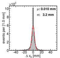
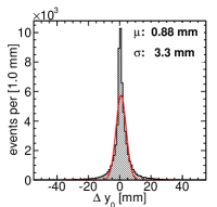
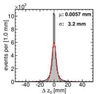
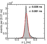
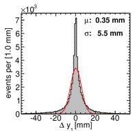
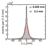
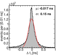
Figure 4: Histograms of $\Delta x_{0}$, $\Delta y_{0}$, $\Delta z_{0}$, $\Delta t_{0}$, representing the accuracy of the primary reconstructed quantities for the first neutron interaction.

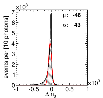
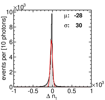
Figure 5: Histograms of $\Delta n_{0}$, $\Delta n_{1}$, representing the number of photons assigned to each interaction by the reconstruction, from which the deposited energy is calculated.

The $\Delta$-histograms of the distance $d_{10}$ and time $t_{10}$ between the first and the second interaction, plotted in Fig. 6, are more relevant quantities for the event reconstruction, as the individual positions and times do not appear in the kinematic equations. The cores of these distributions are thought to represent well reconstructed events and show Gaussian standard deviation values of $7.1~{}\text{mm}$ and $170~{}\text{ps}$. These quantities are derived respectively from combining the coordinates and times of the two interactions, which are not independent variables but instead are correlated by the reconstruction algorithm. Therefore, the asymmetric non-Gaussian tails of the $\Delta d_{10}$ and $\Delta t_{10}$ histograms reveal correlations in the misreconstruction of the individual interaction variables, and their impact on the reconstruction algorithm limits is discussed below. Also included in Fig. 6 is the $\Delta$-histogram of the energy deposited by the first recoiling proton, $E_{\text{p}}$, calculated from $n_{0}$. The quantities $E_{\text{p}}$, $d_{10}$, and $t_{10}$ constitute the inputs used to calculate the incoming neutron energy $E_{\text{n}}$ and scattering angle $\theta$ according to Eqs. 1–3.

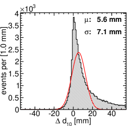
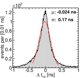
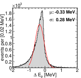
Figure 6: Histograms of the intermediate derived quantities $\Delta d_{10}$, $\Delta t_{10}$, $\Delta E_{\text{p}}$.

In order to evaluate the effect of the event reconstruction in the final reconstruction of the source spectrum and image, the histograms of $\Delta E_{\text{n}}$ and $\Delta\theta$ are plotted in Fig. 7. We also plot the histogram of the angular difference $\Delta\alpha$ between the reconstructed and the true vector defining the axis of the incoming neutron cone, since errors in the cone axis direction will also effect the image reconstruction along with errors in the cone opening angle $\theta$. Note that $\Delta\alpha$ is unique among these resolution plots in being an unsigned angular difference, and consequently we do not expect a symmetric distribution peaked at zero; therefore we do not include a Gaussian fit for $\Delta\alpha$. As for a Rayleigh distribution, we use the mode of the distribution as an estimate of the underlying angular uncertainty in each of two independent orthogonal components; this is the value given in Table 2. However, it should be noted that the $\Delta\alpha$ distribution has a much longer tail than the corresponding Rayleigh distribution, so as in the case of the Gaussian widths, this value at best represents the “core” of well reconstructed events.

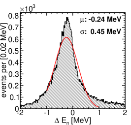
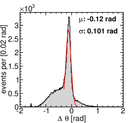
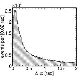
Figure 7: Histograms of the final derived quantities used for spectrum and image reconstruction: $\Delta E_{\text{n}}$, $\Delta\theta$, $\Delta\alpha$.

The most salient feature of these histograms is the broad peak for negative values of $\Delta\theta$ representing reconstructed scattering angles smaller than the true angles. These misreconstructed events correlate with the extended high tail of $\Delta\alpha$ values, as well as other tails in the previous plots of reconstructed quantities. Further investigation indicated that these misreconstructed events are primarily observed when the distance between the first two neutron interactions in the scintillator is small, i.e. less than about $1.5~{}\text{cm}$. Figure 8 shows $\Delta\theta$ as well as $\Delta d_{10}$ plotted against the true $d_{10}$ value, illustrating that result. These events also of course tend to have small time difference between the first two interactions. One likely explanation for this observation, as mentioned above, is that when the first two interactions are close in space and time, they are reconstructed as a single interaction; the reconstruction algorithm then identifies a subsequent interaction or group of interactions as the second one.

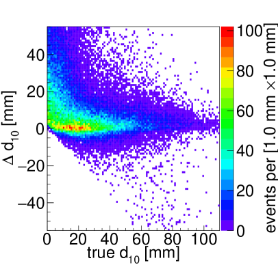
Figure 8: Histograms of $\Delta\theta$ vs true $d_{10}$, and $\Delta d_{10}$ vs true $d_{10}$. These plots demonstrate that most of the misreconstructed events discussed in the text occur when the first two neutron interactions are close together ($<1.5~{}\text{cm}$).

Figure 9 provides a graphical comparison of the effect that smearing the photon time ($T$) and position coordinates $(X,Y,Z)$ have in the reconstruction quality, also showing the intermediate cases in which only time or only position resolutions were applied. The figure demonstrates that the time resolution is the main contributor to the error in event reconstruction; it also reduces the reconstruction success rate by 20%–30%. In contrast, the smearing in photon detection position within the pixel size of currently available MCP- PMT technology has little impact on the event reconstruction. However, the pixel size drives not only position uncertainty but also photon occupancy per pixel, which does not affect these results but will be an important consideration for a hardware implementation.

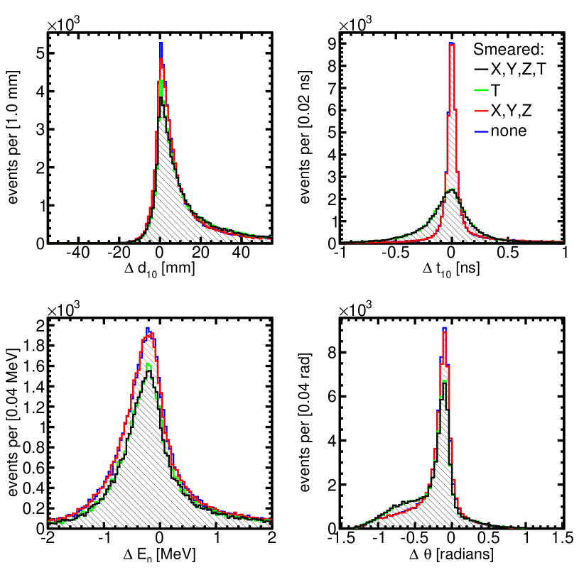
Figure 9: Histograms comparing the reconstruction performance with photodetector spatial and temporal resolution included and excluded from the reconstruction inputs. Upper left: $\Delta d_{10}$. Upper right: $\Delta t_{10}$. Lower left: $\Delta E_{\text{n}}$. Lower right: $\Delta\theta$.

Furthermore, when exact photon times are used, the negative tail in the $\Delta\theta$ histogram decreases in size, and events with the first two interactions as close as $\sim 1~{}\text{cm}$ and $\sim 0.6~{}\text{ns}$ can be successfully reconstructed. While this indicates that reduction in the photon detection time resolution beyond $0.1~{}\text{ns}$ can potentially improve the SVSC performance further, it also establishes an intrinsic limit in event reconstruction resolution within this algorithm framework.

Finally, we consider the highest-level reconstructed distributions, the energy spectrum and image. A reconstructed source energy spectrum is presented in Fig. 10, where it is compared with the “true” spectrum calculated using the known true values of the interactions’ location, time and deposited energy, as well as with the actual incident energy spectrum of the same set of events. The latter two distributions are quite similar albeit with some differences at low $E_{\text{n}}$, but the reconstructed energy spectrum has two qualitative issues. First, for the accurately reconstructed events in the core of the spectrum, $E_{\text{n}}$ is biased low due to the absence of a correction for optical attenuation as discussed above. Second, there is a long tail of misreconstructed events with high $E_{\text{n}}$; in fact, fully 20% of the reconstructed events overflow this plot ($E_{\text{n}}>20~{}\text{MeV}$).

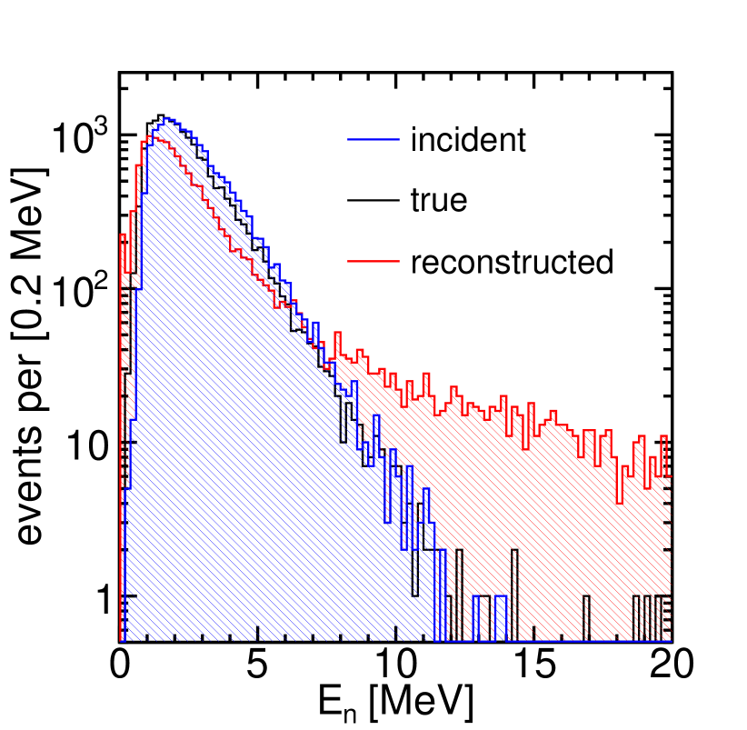
Figure 10: Reconstructed neutron energy spectrum for the simulated ${}^{252}\text{Cf}$ source. The red spectrum is derived from the reconstructed quantities, while the black spectrum is, for the same events, the spectrum that would be calculated from the true positions and times of the first two proton recoils above threshold and the true energy deposited by the first. Both spectra are sculpted by event selection requirements, and by errant event topology such as a carbon scatter between the first two hydrogen scatters. Also included is the spectrum of the actual energy of the incident neutrons of the same events entering the previous two spectra, which is sculpted by the same event selection but not topological effects.

The reconstructed image of Fig. 11 shows good agreement with the simulated source location, indicated by a black cross in the lower zoomed-in view. In the case of the image, misreconstructed events tend to contribute randomly, which reduces their importance in determining a source centroid. This image was reconstructed with list-mode MLEM under the assumption of a simple system response, in which for example the two reconstructed interactions are always taken to be the first two neutron interactions. This method produces qualitatively better results than simple backprojection. However, we expect that further improvements could be obtained in the future with a more complete system response function, including better treatment of experimental resolutions and alternate event topologies, such as, for example, including the possility of an initial carbon scatter. Quantification of the SVSC image quality for point and extended sources will be done in future work.

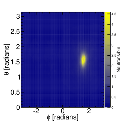
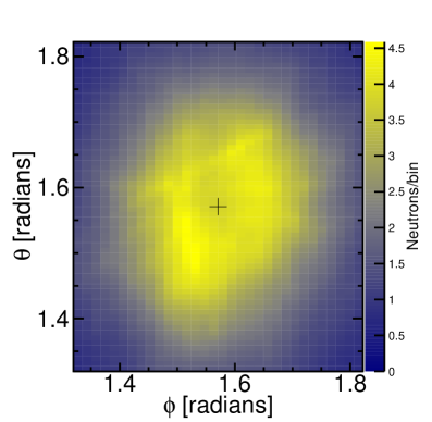
Figure 11: Reconstructed image for the simulated ${}^{252}\text{Cf}$ source. Top: image reconstructed over the full $4\pi$ space. Bottom: zoomed in to the centroid region. The black cross represents the simulated source location. The color scale indicates the number of imaged neutrons from each bin in this source space; there are $400\times 400$ bins in the two-dimensional image.

6 Conclusions

We have described the theoretical advantages of single-volume double-scatter neutron imaging, namely a high imaging efficiency and a compact form factor. We also demonstrated the feasibility of the direct reconstruction SVSC concept via Monte Carlo simulation and reconstruction of a neutron point source.

For the simulated detector system, the results indicate about 13.6% of incident fission-energy neutrons result in at least two proton scattering interactions above $300~{}\text{keV}$, with about half of those events successfully reconstructed using the described event likelihood maximization algorithm. A core resolution of $3~{}\text{mm}$ ($5~{}\text{mm}$) in each spatial dimension and $80~{}\text{ps}$ ($150~{}\text{ps}$) in time is observed for the first (second) interaction, while a limitation of the current likelihood expression results in a bias in the reconstructed number of photons for each interaction. Resolutions of higher-level quantities, such as the distance between the two interactions, have complicated distributions, indicating the presence of non-trivial correlations among the low-level quantitites.

Most of the poorly reconstructed events have small distance (and time) between the two first interactions; this is expected both because these events are more difficult to reconstruct and because, even for a given spatial/temporal resolution, they contain less neutron energy and direction information due to the reduced lever arm.

The response of the system to gammas has not been addressed here, but is an important part of ongoing simulation studies. In particular we would like to understand the ability of the system to discriminate neutron from gamma events based on interaction timing in the absence of pulse shape discrimination.

Physical construction, calibration, and operation of the simulated system presents several technical challenges, and the next desired step is demonstration of the SVSC concept in a laboratory prototype system.

References

References

-
[1]
J. Ryan, K. Bennett, H. Debrunner, D. Forrest, J. Lockwood, M. Loomis,
M. McConnell, D. Morris, V. Schönfelder, B. Swanenburg, W. Webber,
Comptel
measurements of solar flare neutrons, Advances in Space Research 13 (9)
(1993) 255 – 258.
doi:10.1016/0273-1177(93)90487-V.
URL http://www.sciencedirect.com/science/article/pii/027311779390487V -
[2]
P. E. Vanier, Analogies between
neutron imaging and gamma-ray imaging, in: Proc.SPIE, Vol. 6319, 2006, pp.
6319 – 6319 – 8.
doi:10.1117/12.682717.
URL http://dx.doi.org/10.1117/12.682717 - [3] P. Marleau, J. Brennan, K. Krenz, N. Mascarenhas, S. Mrowka, Advances in imaging fission neutrons with a neutron scatter camera, in: 2007 IEEE Nuclear Science Symposium Conference Record, Institute of Electrical & Electronics Engineers (IEEE), 2007, pp. 170–172. doi:10.1109/nssmic.2007.4436310.
-
[4]
J. E. M. Goldsmith, M. D. Gerling, J. S. Brennan,
A compact neutron scatter camera
for field deployment, Review of Scientific Instruments 87 (8) (2016) 083307.
arXiv:http://dx.doi.org/10.1063/1.4961111, doi:10.1063/1.4961111.
URL http://dx.doi.org/10.1063/1.4961111 -
[5]
A. Poitrasson-Rivière, M. C. Hamel, J. K. Polack, M. Flaska, S. D.
Clarke, S. A. Pozzi,
Dual-particle
imaging system based on simultaneous detection of photon and neutron
collision events, Nuclear Instruments and Methods in Physics Research
Section A: Accelerators, Spectrometers, Detectors and Associated Equipment
760 (Supplement C) (2014) 40–45.
doi:10.1016/j.nima.2014.05.056.
URL http://www.sciencedirect.com/science/article/pii/S0168900214005889 -
[6]
N. Mascarenhas, J. Brennan, K. Krenz, P. Marleau, S. Mrowka,
Results
With the Neutron Scatter Camera, IEEE Transactions on Nuclear Science
56 (3) (2009) 1269–1273.
doi:10.1109/TNS.2009.2016659.
URL http://ieeexplore.ieee.org/lpdocs/epic03/wrapper.htm?arnumber=5076056 -
[7]
J. Brennan, E. Brubaker, R. Cooper, M. Gerling, C. Greenberg, P. Marleau,
N. Mascarenhas, S. Mrowka,
Measurement
of the fast neutron energy spectrum of an source using a
neutron scatter camera, IEEE Transactions on Nuclear Science 58 (5) (2011)
2426–2430.
doi:10.1109/TNS.2011.2163192.
URL http://ieeexplore.ieee.org/lpdocs/epic03/wrapper.htm?arnumber=6012498 - [8] K. Weinfurther, J. Mattingly, E. Brubaker, J. Steele, Model-based design evaluation of a compact, high-efficiency neutron scatter camera, Nuclear Instruments and Methods in Physics Research Section A: Accelerators, Spectrometers, Detectors and Associated Equipment 883 (2018) 115–135. arXiv:1710.06480v1, doi:10.1016/j.nima.2017.11.025.
-
[9]
P. Križan,
Overview
of photon detectors for fast single photon detection, Journal of
Instrumentation 9 (10) (2014) C10010–C10010.
doi:10.1088/1748-0221/9/10/C10010.
URL http://stacks.iop.org/1748-0221/9/i=10/a=C10010?key=crossref.dd2d276bf48d2aec459f867b12392922 -
[10]
J. L. Wiza, Microchannel
plate detectors, Nuclear Instruments and Methods 162 (1-3) (1979) 587–601.
doi:10.1016/0029-554x(79)90734-1.
URL http://dx.doi.org/10.1016/0029-554X(79)90734-1 -
[11]
H. Kim, C.-T. Chen, H. Frisch, F. Tang, C.-M. Kao,
A prototype TOF PET
detector module using a micro-channel plate photomultiplier tube with
waveform sampling, Nuclear Instruments and Methods in Physics Research
Section A: Accelerators, Spectrometers, Detectors and Associated Equipment
662 (1) (2012) 26–32.
doi:10.1016/j.nima.2011.09.059.
URL http://dx.doi.org/10.1016/j.nima.2011.09.059 -
[12]
V. A. Li, R. Dorrill, M. J. Duvall, J. Koblanski, S. Negrashov, M. Sakai, S. A.
Wipperfurth, K. Engel, G. R. Jocher, J. G. Learned, L. Macchiarulo,
S. Matsuno, W. F. McDonough, H. P. Mumm, J. Murillo, K. Nishimura, M. Rosen,
S. M. Usman, G. S. Varner, Invited
article: miniTimeCube, Review of Scientific Instruments 87 (2) (2016)
021301.
doi:10.1063/1.4942243.
URL https://doi.org/10.1063/1.4942243 - [13] A. R. Back, J. F. Beacom, M. Bergevin, E. Catano-Mur, S. Dazeley, E. Drakopoulou, F. D. Lodovico, A. Elagin, J. Eisch, V. Fischer, S. Gardiner, R. Hatcher, J. He, R. Hill, T. Katori, F. Krennrich, R. Kreymer, M. Malek, C. L. McGivern, M. Needham, M. O’Flaherty, G. D. O. Gann, B. Richards, M. C. Sanchez, M. Smy, R. Svoboda, E. Tiras, M. Vagins, J. Wang, A. Weinstein, M. Wetstein, Accelerator Neutrino Neutron Interaction Experiment (ANNIE): Preliminary results and physics phase proposal, Tech. rep., Iowa State University (2017). arXiv:1707.08222v2.
- [14] Photonis, Planacon XP-85012 Data Sheet (January 2013).
-
[15]
B. Adams, A. Elagin, H. Frisch, R. Obaid, E. Oberla, A. Vostrikov, R. Wagner,
J. Wang, M. Wetstein,
Timing characteristics of
large area picosecond photodetectors, Nuclear Instruments and Methods in
Physics Research Section A: Accelerators, Spectrometers, Detectors and
Associated Equipment 795 (2015) 1–11.
doi:10.1016/j.nima.2015.05.027.
URL http://dx.doi.org/10.1016/j.nima.2015.05.027 -
[16]
S. A. Pozzi, E. Padovani, M. Marseguerra,
Mcnp-polimi:
a monte-carlo code for correlation measurements, Nuclear Instruments and
Methods in Physics Research Section A: Accelerators, Spectrometers, Detectors
and Associated Equipment 513 (3) (2003) 550 – 558.
doi:10.1016/j.nima.2003.06.012.
URL http://www.sciencedirect.com/science/article/pii/S0168900203023027 -
[17]
K. Ziock, J. Braverman, L. Fabris, M. Harrison, D. Hornback, J. Newby,
Event
localization in bulk scintillator crystals using coded apertures, Nuclear
Instruments and Methods in Physics Research Section A: Accelerators,
Spectrometers, Detectors and Associated Equipment 784 (Supplement C) (2015)
382 – 389, symposium on Radiation Measurements and Applications 2014 (SORMA
XV).
doi:https://doi.org/10.1016/j.nima.2015.01.013.
URL http://www.sciencedirect.com/science/article/pii/S016890021500039X - [18] C. Lane, S. M. Usman, J. Blackmon, C. Rasco, H. P. Mumm, D. Markoff, G. R. Jocher, R. Dorrill, M. Duvall, J. G. Learned, V. Li, J. Maricic, S. Matsuno, R. Milincic, S. Negrashov, M. Sakai, M. Rosen, G. Varner, P. Huber, M. L. Pitt, S. D. Rountree, R. B. Vogelaar, T. Wright, Z. Yokley, A new type of neutrino detector for sterile neutrino search at nuclear reactors and nuclear nonproliferation applications, ArxivarXiv:1501.06935v1.
-
[19]
S. Ritt, R. Dinapoli, U. Hartmann,
Application
of the DRS chip for fast waveform digitizing, Nuclear Instruments and
Methods in Physics Research Section A: Accelerators, Spectrometers, Detectors
and Associated Equipment (2010) 1–3doi:10.1016/j.nima.2010.03.045.
URL http://linkinghub.elsevier.com/retrieve/pii/S0168900210006091 -
[20]
M. Bitossi, R. Paoletti, D. Tescaro,
Ultra-fast sampling and
data acquisition using the drs4 waveform digitizer, IEEE Transactions on
Nuclear Science 63 (4) (2016) 2309 – 2316.
doi:10.1109/TNS.2016.2578963.
URL http://dx.doi.org/10.1109/TNS.2016.2578963 -
[21]
E. Oberla, J.-F. Genat, H. Grabas, H. Frisch, K. Nishimura, G. Varner,
A 15GSa/s, 1.5GHz
bandwidth waveform digitizing ASIC, Nuclear Instruments and Methods in
Physics Research Section A: Accelerators, Spectrometers, Detectors and
Associated Equipment 735 (2014) 452–461.
arXiv:1309.4397v1,
doi:10.1016/j.nima.2013.09.042.
URL http://dx.doi.org/10.1016/j.nima.2013.09.042 - [22] E. Technology, Ej-232Q Data Sheet.
-
[23]
R. Barlow,
Extended
maximum likelihood, Nuclear Instruments and Methods in Physics Research
Section A: Accelerators, Spectrometers, Detectors and Associated Equipment
297 (3) (1990) 496 – 506.
doi:https://doi.org/10.1016/0168-9002(90)91334-8.
URL http://www.sciencedirect.com/science/article/pii/0168900290913348 - [24] F. James, MINUIT Function Minimization and Error Analysis: Reference Manual Version 94.1, Tech. rep., CERN (1994).
-
[25]
L. A. Shepp, Y. Vardi,
Maximum likelihood
reconstruction for emission tomography., IEEE transactions on medical
imaging 1 (2) (1982) 113–22.
doi:10.1109/TMI.1982.4307558.
URL http://www.ncbi.nlm.nih.gov/pubmed/18238264 -
[26]
S. Agostinelli, J. Allison, K. Amako, J. Apostolakis, H. Araujo, P. Arce,
M. Asai, D. Axen, S. Banerjee, G. Barrand, F. Behner, L. Bellagamba,
J. Boudreau, L. Broglia, A. Brunengo, H. Burkhardt, S. Chauvie, J. Chuma,
R. Chytracek, G. Cooperman, G. Cosmo, P. Degtyarenko,
A. Dell'Acqua, G. Depaola, D. Dietrich, R. Enami,
A. Feliciello, C. Ferguson, H. Fesefeldt, G. Folger, F. Foppiano, A. Forti,
S. Garelli, S. Giani, R. Giannitrapani, D. Gibin, J. G. Cadenas,
I. González, G. G. Abril, G. Greeniaus, W. Greiner, V. Grichine,
A. Grossheim, S. Guatelli, P. Gumplinger, R. Hamatsu, K. Hashimoto, H. Hasui,
A. Heikkinen, A. Howard, V. Ivanchenko, A. Johnson, F. Jones, J. Kallenbach,
N. Kanaya, M. Kawabata, Y. Kawabata, M. Kawaguti, S. Kelner, P. Kent,
A. Kimura, T. Kodama, R. Kokoulin, M. Kossov, H. Kurashige, E. Lamanna,
T. Lampén, V. Lara, V. Lefebure, F. Lei, M. Liendl, W. Lockman,
F. Longo, S. Magni, M. Maire, E. Medernach, K. Minamimoto, P. M. de Freitas,
Y. Morita, K. Murakami, M. Nagamatu, R. Nartallo, P. Nieminen, T. Nishimura,
K. Ohtsubo, M. Okamura, S. O'Neale, Y. Oohata, K. Paech,
J. Perl, A. Pfeiffer, M. Pia, F. Ranjard, A. Rybin, S. Sadilov, E. D. Salvo,
G. Santin, T. Sasaki, N. Savvas, Y. Sawada, S. Scherer, S. Sei, V. Sirotenko,
D. Smith, N. Starkov, H. Stoecker, J. Sulkimo, M. Takahata, S. Tanaka,
E. Tcherniaev, E. S. Tehrani, M. Tropeano, P. Truscott, H. Uno, L. Urban,
P. Urban, M. Verderi, A. Walkden, W. Wander, H. Weber, J. Wellisch,
T. Wenaus, D. Williams, D. Wright, T. Yamada, H. Yoshida, D. Zschiesche,
Geant4—a
simulation toolkit, Nuclear Instruments and Methods in Physics Research
Section A: Accelerators, Spectrometers, Detectors and Associated Equipment
506 (3) (2003) 250–303.
doi:10.1016/s0168-9002(03)01368-8.
URL http://dx.doi.org/10.1016/S0168-9002(03)01368-8 -
[27]
S. A. Pozzi, J. A. Mullens, J. T. Mihalczo,
Analysis
of neutron and photon detection position for the calibration of plastic
(bc-420) and liquid (bc-501) scintillators, Nuclear Instruments and Methods
in Physics Research Section A: Accelerators, Spectrometers, Detectors and
Associated Equipment 524 (1) (2004) 92 – 101.
doi:10.1016/j.nima.2003.12.036.
URL http://www.sciencedirect.com/science/article/pii/S0168900204001342 -
[28]
R. Batchelor, W. Gilboy, J. Parker, J. Towle,
The response of organic
scintillators to fast neutrons, Nuclear Instruments and Methods 13 (1961)
70–82.
doi:10.1016/0029-554x(61)90171-9.
URL http://dx.doi.org/10.1016/0029-554X(61)90171-9 -
[29]
S. N. Kasarova, N. G. Sultanova, C. D. Ivanov, I. D. Nikolov,
Analysis
of the dispersion of optical plastic materials, Optical Materials 29 (11)
(2007) 1481 – 1490.
doi:10.1016/j.optmat.2006.07.010.
URL http://www.sciencedirect.com/science/article/pii/S0925346706002473 -
[30]
V. A. Grigoryev, V. A. Kaplin, T. L. Karavicheva, A. B. Kurepin, E. F.
Maklyaev, Y. A. Melikyan, D. V. Serebryakov, W. H. Trzaska, E. M. Tykmanov,
Study of the planacon
xp85012 photomultiplier characteristics for its use in a cherenkov detector,
Journal of Physics: Conference Series 675 (4) (2016) 042016.
URL http://stacks.iop.org/1742-6596/675/i=4/a=042016