CERN-TH-2018-029

IFT-UAM/CSIC-18-011

FTUAM-18-4

Non-perturbative quark mass renormalisation and running in $N_{\mathrm{\scriptstyle f}}=3$ QCD

I. Campos^a, P. Fritzsch^b, C. Pena^c, D. Preti^d, A. Ramos^e, A. Vladikas^f

^a Instituto de Física de Cantabria IFCA-CSIC

Avda. de los Castros s/n, E-39005 Santander, Spain

^b Theoretical Physics Department, CERN

CH-1211 Geneva 23, Switzerland

^c Instituto de Física Teórica UAM-CSIC &

Dpto. de Física Teórica, Universidad Autónoma de Madrid

Cantoblanco E-28049 Madrid, Spain

^d INFN, Sezione di Torino

Via Pietro Giuria 1, I-10125 Turin, Italy

^e School of Mathematics, Trinity College Dublin

Dublin 2, Ireland

^f INFN, Sezione di Tor Vergata

c/o Dipartimento di Fisica, Università di Roma “Tor Vergata”

Via della Ricerca Scientifica 1, I-00133 Rome, Italy

Abstract: We determine from first principles the quark mass anomalous dimension in $N_{\mathrm{\scriptstyle f}}=3$ QCD between the electroweak and hadronic scales. This allows for a fully non-perturbative connection of the perturbative and non-perturbative regimes of the Standard Model in the hadronic sector. The computation is carried out to high accuracy, employing massless $\mbox{O}(a)$-improved Wilson quarks and finite-size scaling techniques. We also provide the matching factors required in the renormalisation of light quark masses from lattice computations with $\mbox{O}(a)$-improved Wilson fermions and a tree-level Symanzik improved gauge action. The total uncertainty due to renormalisation and running in the determination of light quark masses in the SM is thus reduced to about $1\%$.

1 Introduction

In the paradigm provided by the Standard Model (SM) of Particle Physics, quark masses are fundamental constants of Nature. More specifically, Quantum Chromodynamics (QCD), the part of the SM that describes the fundamental strong interaction, is uniquely defined by the values of the quark masses and the strong coupling constant. Apart from this intrinsic interest, precise knowledge of the values of quark masses is crucial for the advancement of frontier research in particle physics — one good illustration being the fact that the values of the bottom and charm quark masses are major sources of uncertainty in several important Higgs branching fractions, e.g., $\Gamma(H\to b\bar{b})$ and $\Gamma(H\to c\bar{c})$ [1, 2, 3, 4, 5].

Quark masses are couplings in the QCD Lagrangian, and have to be treated within a consistent definition of the renormalised theory. A meaningful determination can only be achieved by computing physical observables as a function of quark masses, and matching the result to the experimental values. A non-perturbative treatment of QCD is mandatory to avoid the presence of unquantified systematic uncertainties in such a computation: the asymptotic nature of the perturbative series, and the strongly coupled nature of the interaction at typical hadronic energy scales, implies the presence of an irreducible uncertainty in any determination that does not treat long-distance strong interaction effects from first principles. Lattice QCD (LQCD) is therefore the best-suited framework for a high-precision determination of quark masses. Indeed, following the onset of the precision era in LQCD, the uncertainties on the values of both light and heavy quark masses have dramatically decreased in recent years [6, 7, 8, 9, 10, 11, 12, 13, 14, 15, 16, 17, 18, 19, 20, 21, 22].

The natural observables employed in a LQCD computation of quark masses are hadronic quantities, considered at energy scales around or below $1~{}{\rm GeV}$. This requires, in particular, to work out the renormalisation non-perturbatively. Then, in order to make contact with the electroweak scale, where the masses are used to compute the QCD contribution to high-energy observables, the masses have to be run with the Renormalisation Group (RG) across more than two orders of magnitude in energy. While high-order perturbative estimates of the anomalous dimension of quark masses in various renormalisation schemes exist [23, 24, 25], a non-perturbative determination is mandatory to match the current percent-level precision of the relevant hadronic observables.

In this work we present a high-precision determination of the anomalous dimension of quark masses in QCD with three light quark flavours, as well as of the renormalisation constants required to match bare quark masses. This is a companion project of the recent high-precision determination of the $\beta$ function and the $\Lambda_{\rm\scriptscriptstyle QCD}$ parameter in $N_{\mathrm{\scriptstyle f}}=3$ QCD by the ALPHA Collaboration [29, 30, 31, 32]. We will employ the Schrödinger Functional [33, 34] as an intermediate renormalisation scheme that allows to make contact between the hadronic scheme used in the computation of bare quark masses and the perturbative schemes used at high energies, and employ well-established finite-size recursion techniques [35, 36, 37, 38, 39, 40, 41, 42, 43, 44, 45, 46] to compute the RG running non-perturbatively. Our main result is a high-precision determination of the mass anomalous dimension between the electroweak scale and hadronic scales at around $200~{}{\rm MeV}$, where contact with hadronic observables obtained from simulations by the CLS effort [47] can be achieved.

The paper is structured as follows. In Section 2 we describe our strategy, which (similar to the determination of $\Lambda_{\rm\scriptscriptstyle QCD}$) involves using two different definitions of the renormalised coupling at energies above and below an energy scale around $2~{}{\rm GeV}$. Sections 3 and 4 deal with the determination of the anomalous dimension above and below that scale, respectively. Section 5 discusses the determination of the renormalisation constants needed to match to a hadronic scheme at low energies. Conclusions and outlook come in Section 6. Several technical aspects of the work are discussed in appendices.

2 Strategy

2.1 Quark running and RGI masses

QCD is a theory with $N_{\mathrm{\scriptstyle f}}+1$ parameters: the coupling constant $g$ and the $N_{\mathrm{\scriptstyle f}}$ quark masses $\{m_{i},\,i=1,\ldots,N_{\mathrm{\scriptstyle f}}\}$. When the theory is defined using some regularisation, $g$ and $m_{i}$ are taken to be the bare parameters appearing in the Lagrangian. Removing the regularisation requires to define renormalised parameters $\kern 1.0pt\overline{\kern-1.0ptg\kern 0.0pt}\kern 1.0pt,\{\kern 2.0pt\overline{\kern-1.0ptm\kern-1.0pt}\kern 1.0pt_{i},\,i=1,\ldots,N_{\mathrm{\scriptstyle f}}\}$ at some energy scale $\mu$. In the following we will assume the use of renormalisation conditions that are independent of the values of the quark masses, which leads to mass-independent renormalisation schemes. The renormalised parameters are then functions of the renormalisation scale $\mu$ alone [48, 49], and their scale evolution is given by renormalisation group equations of the form

$$\mu\frac{{\rm d}}{{\rm d}\mu}\,\kern 1.0pt\overline{\kern-1.0ptg\kern 0.0pt}\kern 1.0pt(\mu) =\beta(\kern 1.0pt\overline{\kern-1.0ptg\kern 0.0pt}\kern 1.0pt(\mu))\,,$$ (2.1)

$$\mu\frac{{\rm d}}{{\rm d}\mu}\,\kern 2.0pt\overline{\kern-1.0ptm\kern-1.0pt}\kern 1.0pt_{i}(\mu) =\tau(\kern 1.0pt\overline{\kern-1.0ptg\kern 0.0pt}\kern 1.0pt(\mu))\,\kern 2.0pt\overline{\kern-1.0ptm\kern-1.0pt}\kern 1.0pt_{i}(\mu)\,,\qquad i=1,\ldots,N_{\mathrm{\scriptstyle f}}\,.$$ (2.2)

The renormalisation group functions $\beta$ and $\tau$ admit perturbative expansions of the form

$$\beta(g) \underset{g\to 0}{\sim}-g^{3}(b_{0}+b_{1}g^{2}+b_{2}g^{4}+\ldots)\,,$$ (2.3)

$$\tau(g) \underset{g\to 0}{\sim}-g^{2}(d_{0}+d_{1}g^{2}+d_{2}g^{4}+\ldots)\,,$$ (2.4)

with universal coefficients given by [50, 51, 52, 53, 54, 55, 56]

$$b_{0} =\frac{1}{(4\pi)^{2}}\left(11-\frac{2}{3}N_{\mathrm{\scriptstyle f}}\right)\,,\quad b_{1}=\frac{1}{(4\pi)^{4}}\left(102-\frac{38}{3}N_{\mathrm{\scriptstyle f}}\right)\,,$$ (2.5)

$$d_{0} =\frac{8}{(4\pi)^{2}}\,.$$ (2.6)

The higher-order coefficients $b_{n\geq 2},~{}d_{n\geq 1}$ are instead renormalisation scheme-dependent. It is trivial to integrate Eqs. (2.1,2.2) formally, to obtain the renormalisation group invariants (RGI)

$$\Lambda_{\rm\scriptscriptstyle QCD} =\mu\left[b_{0}\kern 1.0pt\overline{\kern-1.0ptg\kern 0.0pt}\kern 1.0pt^{2}(\mu)\right]^{-\frac{b_{1}}{2b_{0}^{2}}}\,e^{-\frac{1}{2b_{0}\kern 1.0pt\overline{\kern-1.0ptg\kern 0.0pt}\kern 1.0pt^{2}(\mu)}}\,\exp\left\{-\int_{0}^{\kern 1.0pt\overline{\kern-1.0ptg\kern 0.0pt}\kern 1.0pt(\mu)}{\rm d}g\left[\frac{1}{\beta(g)}+\frac{1}{b_{0}g^{3}}-\frac{b_{1}}{b_{0}^{2}g}\right]\right\}\,,$$ (2.7)

$$M_{i} =\kern 2.0pt\overline{\kern-1.0ptm\kern-1.0pt}\kern 1.0pt_{i}(\mu)\left[2b_{0}\kern 1.0pt\overline{\kern-1.0ptg\kern 0.0pt}\kern 1.0pt^{2}(\mu)\right]^{-\frac{d_{0}}{2b_{0}}}\exp\left\{-\int_{0}^{\kern 1.0pt\overline{\kern-1.0ptg\kern 0.0pt}\kern 1.0pt(\mu)}{\rm d}g\left[\frac{\tau(g)}{\beta(g)}-\frac{d_{0}}{b_{0}g}\right]\right\}\,.$$ (2.8)

Note that the integrands are finite at $g=0$, making the integrals well defined (and zero at universal order in perturbation theory). Note also that $\Lambda_{\rm\scriptscriptstyle QCD}$ and $M_{i}$ are non-perturbatively defined via the previous expressions. It is easy to check, furthermore, that they are $N_{\mathrm{\scriptstyle f}}$-dependent but $\mu$-independent. They can be interpreted as the integration constants of the renormalisation group equations. Also the ratios $\kern 2.0pt\overline{\kern-1.0ptm\kern-1.0pt}\kern 1.0pt_{i}(\mu)/\kern 2.0pt\overline{\kern-1.0ptm\kern-1.0pt}\kern 1.0pt_{j}(\mu),\,i\neq j$ are scale-independent. Furthermore, the ratios $M_{i}/\kern 2.0pt\overline{\kern-1.0ptm\kern-1.0pt}\kern 1.0pt_{i}(\mu)$ are independent of the quark flavour $i$, due to the mass-independence of the quark mass anomalous dimension $\tau$. Finally, the values of $M_{i}$ can be easily checked to be independent of the renormalisation scheme. The value of $\Lambda_{\rm\scriptscriptstyle QCD}$ is instead scheme-dependent, but the ratio $\Lambda_{\rm\scriptscriptstyle QCD}/\Lambda_{\rm\scriptscriptstyle QCD}^{\prime}$ between its values in two different schemes can be calculated exactly using one-loop perturbation theory.

2.2 Step scaling functions

In our computation, we will access the renormalisation group functions $\beta$ and $\tau$ through the quantities $\sigma$ and $\sigma_{\rm\scriptscriptstyle P}$, defined as

$$\ln 2 =-\int_{\sqrt{u}}^{\sqrt{\sigma(u)}}\kern 0.0pt{\rm d}g\,\frac{1}{\beta(g)}\,,$$ (2.9a)

$$\sigma_{\rm\scriptscriptstyle P}(u) =\exp\left\{-\int_{\sqrt{u}}^{\sqrt{\sigma(u)}}\kern 0.0pt{\rm d}g\,\frac{\tau(g)}{\beta(g)}\right\}\,,$$ (2.9b)

and to which we will refer as coupling and mass step scaling functions (SSFs), respectively. They correspond to the renormalisation group evolution operators for the coupling and quark mass between scales that differ by a factor of two, viz.

$$\sigma(u)=\left.\kern 1.0pt\overline{\kern-1.0ptg\kern 0.0pt}\kern 1.0pt^{2}(\mu/2)\right|_{u=\kern 1.0pt\overline{\kern-1.0ptg\kern 0.0pt}\kern 1.0pt^{2}(\mu)}\,,\qquad\sigma_{\rm\scriptscriptstyle P}(u)=\left.\frac{\kern 2.0pt\overline{\kern-1.0ptm\kern-1.0pt}\kern 1.0pt_{i}(\mu)}{\kern 2.0pt\overline{\kern-1.0ptm\kern-1.0pt}\kern 1.0pt_{i}(\mu/2)}\right|_{u=\kern 1.0pt\overline{\kern-1.0ptg\kern 0.0pt}\kern 1.0pt^{2}(\mu)}\,.$$ (2.10)

The main advantage of these quantities is that they can be computed accurately on the lattice, with a well-controlled continuum limit for a very wide range of energy scales. This is so thanks to the use of finite size scaling techniques, first introduced for quark masses in [35]. The RG functions can be non-perturbatively computed between the hadronic regime and the electroweak scale, establishing safe contact with the asymptotic perturbative regime

In order to compute the SSF $\sigma_{\rm\scriptscriptstyle P}$, we define renormalised quark masses through the partially conserved axial current (PCAC) relation,

$$\partial_{\mu}(A_{\rm R})^{ij}_{\mu}=(\kern 2.0pt\overline{\kern-1.0ptm\kern-1.0pt}\kern 1.0pt_{i}+\kern 2.0pt\overline{\kern-1.0ptm\kern-1.0pt}\kern 1.0pt_{j})P_{\rm R}^{ij}\,,$$ (2.11)

where the renormalised, non-singlet ($i\neq j$) axial current and pseudoscalar density operators are given by

$$(A_{\rm R})^{ij}_{\mu}(x) =Z_{\rm\scriptscriptstyle A}\bar{\psi}_{i}(x)\gamma_{\mu}\gamma_{5}\psi_{j}(x)\,,$$ (2.12)

$$(P_{\rm R})^{ij}(x) =Z_{\rm\scriptscriptstyle P}\bar{\psi}_{i}(x)\gamma_{5}\psi_{j}(x)\,.$$ (2.13)

In these expressions $Z_{\rm\scriptscriptstyle P}$ is the renormalisation constant of the pseudoscalar density in the regularised theory, and $Z_{\rm\scriptscriptstyle A}$ is the finite axial current normalisation, required when the QCD regularisation breaks chiral symmetry, as with lattice Wilson fermions. Eq. (2.11) implies that, up to the finite current normalisation, current quark masses renormalise with $Z_{\rm\scriptscriptstyle P}^{-1}$. Therefore, the SSF $\sigma_{\rm\scriptscriptstyle P}$ of Eq. (2.9b) can be obtained by computing $Z_{\rm\scriptscriptstyle P}$ at fixed bare gauge coupling $g_{0}^{2}$ — i.e., fixed lattice spacing — for scales $\mu$ and $\mu/2$. This is repeated for several different values of the lattice spacing $a$, and the continuum limit of their ratio is taken, viz.

$$\sigma_{\rm\scriptscriptstyle P}(u)=\lim_{a\to 0}\left.\Sigma_{\rm\scriptscriptstyle P}(g_{0}^{2},a\mu)\right|_{\kern 1.0pt\overline{\kern-1.0ptg\kern 0.0pt}\kern 1.0pt^{2}(\mu)=u}\,,\qquad\Sigma_{\rm\scriptscriptstyle P}(g_{0}^{2},a\mu)\equiv\frac{Z_{\rm\scriptscriptstyle P}(g_{0}^{2},a\mu/2)}{Z_{\rm\scriptscriptstyle P}(g_{0}^{2},a\mu)}\,,$$ (2.14)

where $g_{0}^{2}$ is the bare coupling, univocally related to $a$ in mass-independent schemes. The condition that the value of the renormalised coupling $u=\kern 1.0pt\overline{\kern-1.0ptg\kern 0.0pt}\kern 1.0pt^{2}(\mu)$ is kept fixed in the extrapolation ensures that the latter is taken along a line of constant physics.

In this work we will determine non-perturbatively $\tau(\bar{g})$ from Eq. (2.9b). Note that in order to do so, we need the RG function $\beta(\bar{g})$. As we will note later, the non-perturbative determination of the $\beta$ function has already been done in our schemes of choice [29, 31]. In practice, given the $\beta$ function (and hence $\sigma(u)$), and the lattice results for $\Sigma_{\rm\scriptscriptstyle P}(g_{0}^{2},a\mu)$, one determines the anomalous dimension $\tau(\kern 1.0pt\overline{\kern-1.0ptg\kern 0.0pt}\kern 1.0pt)$ by extrapolating $\Sigma_{\rm\scriptscriptstyle P}(u,a\mu)$ to the continuum (Eq. (2.14)) and then using the relation Eq. (2.9b) to constrain the functional form of $\tau(\kern 1.0pt\overline{\kern-1.0ptg\kern 0.0pt}\kern 1.0pt)$.

2.3 Renormalisation schemes

In order to control the connection between hadronic observables and RGI quantities, we will use intermediate finite-volume renormalisation schemes that allow to define fully non-perturbative renormalised gauge coupling and quark masses. For that purpose, $Z_{\rm\scriptscriptstyle P}$ will be defined by a renormalisation condition imposed using the Schrödinger Functional (SF) [33, 34]. In the following, we will adopt the conventions and notations for the lattice SF setup introduced in [57].

SF schemes are based on the formulation of QCD in a finite space-time volume of size $T^{3}\times L$, with inhomogeneous Dirichlet boundary conditions at Euclidean times $x_{0}=0$ and $x_{0}=T$. The boundary condition for gauge fields has the form

$$\left.U_{k}(x)\right|_{x_{0}=0}={\cal P}\exp\left\{a\int_{0}^{1}{\rm d}t\,\,C_{k}(\mathbf{x}+(1-t)a\hat{\mathbf{k}})\right\}\,,$$ (2.15)

where $\hat{\mathbf{k}}$ is a unit vector in the direction $k$, ${\cal P}\exp$ is a path-ordered exponential, and $C_{k}$ is some smooth gauge field. A similar expression applies at $x_{0}=T$ in terms of another field $C^{\prime}_{k}$. Fermion fields obey the boundary conditions

$$\left.P_{+}\psi(x)\right|_{x_{0}=0\,} =\rho(\mathbf{x})\,, \left.\bar{\psi}(x)P_{-}\right|_{x_{0}=0\,} =\bar{\rho}(\mathbf{x})\,,$$ (2.16)

$$\left.P_{-}\psi(x)\right|_{x_{0}=T} =\rho^{\prime}(\mathbf{x})\,, \left.\bar{\psi}(x)P_{+}\right|_{x_{0}=T} =\bar{\rho}^{\prime}(\mathbf{x})\,,$$ (2.17)

with $P_{\pm}={\scriptstyle{{1\over 2}}}(\mathbf{1}\pm\gamma_{0})$. Gauge fields are periodic in spatial directions, whereas fermion fields are periodic up to a global phase

$$\psi(x+L\hat{\mathbf{k}})=e^{i\theta_{k}}\psi(x)\,,\qquad\bar{\psi}(x+L\hat{\mathbf{k}})=\bar{\psi}(x)e^{-i\theta_{k}}\,.$$ (2.18)

The SF is the generating functional

$${\cal Z}[C,\bar{\rho},\rho;C^{\prime},\bar{\rho}^{\prime},\rho^{\prime}]=\int{\rm D}[U]{\rm D}[\psi]{\rm D}[\bar{\psi}]\,e^{-S[U,\bar{\psi},\psi]}\,,$$ (2.19)

where the integral is performed over all fields with the specified boundary values. Expectation values of any product ${\cal O}$ of fields are then given by

$$\langle{\cal O}\rangle=\left\{\frac{1}{{\cal Z}}\int{\rm D}[U]{\rm D}[\psi]{\rm D}[\bar{\psi}]\,{\cal O}e^{-S[U,\bar{\psi},\psi]}\right\}_{\bar{\rho}=\rho=\bar{\rho}^{\prime}=\rho^{\prime}=0}\,,$$ (2.20)

where ${\cal O}$ can involve, in particular, the “boundary fields”

$$\zeta(\mathbf{x})=\frac{\delta}{\delta\rho(\mathbf{x})}\,,\quad\bar{\zeta}(\mathbf{x})=-\frac{\delta}{\delta\bar{\rho}(\mathbf{x})}\,;\qquad\qquad\zeta^{\prime}(\mathbf{x})=\frac{\delta}{\delta\rho^{\prime}(\mathbf{x})}\,,\quad\bar{\zeta}^{\prime}(\mathbf{x})=-\frac{\delta}{\delta\bar{\rho}^{\prime}(\mathbf{x})}\,.$$ (2.21)

The Dirichlet boundary conditions provide an infrared cutoff to the possible wavelengths of quark and gluon fields, which allows to simulate at vanishing quark mass. The presence of non-trivial boundary conditions requires, in general, additional counterterms to renormalise the theory [58, 59, 33]. In the case of the SF, it has been shown in [60] that no additional counterterms are needed with respect to the periodic case, except for one boundary term that amounts to rescaling the boundary values of quark fields by a logarithmically divergent factor, which is furthermore absent if $\bar{\rho}=\rho=\bar{\rho}^{\prime}=\rho^{\prime}=0$. It then follows that the SF is finite after the usual QCD renormalisation.

The SF naturally allows for the introduction of finite-volume renormalisation schemes, where the renormalisation scale is identified with the inverse box length,

$$\mu=\frac{1}{L}\,.$$ (2.22)

The renormalisation of the pseudoscalar density, and hence of quark masses, is treated in the same way as in [35]. We introduce the SF correlation functions

$$f_{\rm\scriptscriptstyle P}(x_{0}) =-\frac{1}{3}\int{\rm d}^{3}x\langle P^{ij}(x)\,{\cal O}^{ji}\rangle\,,$$ (2.23)

$$f_{1} =-\frac{1}{3}\langle{\cal O}^{\prime ij}\,{\cal O}^{ji}\rangle\,,$$ (2.24)

where $P^{ij}$ is the unrenormalised pseudoscalar density, and ${\cal O}$, ${\cal O}^{\prime}$ are operators with pseudoscalar quantum numbers made up of boundary quark fields

$${\cal O}^{ij}=\frac{1}{L^{3}}\int{\rm d}^{3}y\int{\rm d}^{3}z\,\bar{\zeta}_{i}(\mathbf{y})\gamma_{5}\zeta_{j}(\mathbf{z})\,,\quad{\cal O}^{\prime ij}=\frac{1}{L^{3}}\int{\rm d}^{3}y\int{\rm d}^{3}z\,\bar{\zeta}^{\prime}_{i}(\mathbf{y})\gamma_{5}\zeta^{\prime}_{j}(\mathbf{z})\,.$$ (2.25)

The pseudoscalar renormalisation constant is then defined as

$$Z_{\rm\scriptscriptstyle P}\,\frac{f_{\rm\scriptscriptstyle P}(L/2)}{\sqrt{3f_{1}}}=\left.\frac{f_{\rm\scriptscriptstyle P}(L/2)}{\sqrt{3f_{1}}}\right|_{\rm tree~{}level}\,,$$ (2.26)

with all correlation functions computed at zero quark masses. The renormalisation condition is fully specified by fixing the boundary conditions and the box geometry as follows:

$$T=L\,,\qquad C=C^{\prime}=0\,,\qquad\theta_{k}\equiv\theta=\frac{1}{2}\,.$$ (2.27)

Furthermore, for computational convenience (cf. below), all correlation functions will be computed in a fixed topological sector of the theory, chosen to be the one with total topological charge $Q=0$. This is just part of the scheme definition, and does not change the ultraviolet structure of the observables.

In order to completely fix the renormalisation scheme for quark masses, we still need to provide a definition of the renormalised coupling. This allows to relate the scale $\mu=1/L$ to the bare coupling, and hence to the lattice spacing, in an unambiguous way, so that the continuum limit of $\Sigma_{\rm\scriptscriptstyle P}$ is precisely defined. Following [29, 31], we will introduce two different definitions, to be used in qualitatively different regimes. For renormalisation scales larger than some value $\mu_{0}/2$, we will employ the non-perturbative SF coupling first introduced in [33]. Below that scale, we will use the gradient flow (GF) coupling defined in [61]. As discussed in [62], this allows to optimally exploit the variance properties of the couplings, so that a very precise computation of the $\beta$ function, and ultimately of the $\Lambda_{\rm\scriptscriptstyle QCD}$ parameter, is achieved. In our context, the main consequence of this setup is that our quark masses are implicitly defined in two different schemes above and below $\mu_{0}/2$; we will refer to them as ${\rm SF}$ and ${\rm GF}$, respectively. Note that the schemes differ only by the choice of renormalized coupling $\kern 1.0pt\overline{\kern-1.0ptg\kern 0.0pt}\kern 1.0pt^{2}$; the definition of $Z_{\rm\scriptscriptstyle P}$ is always given by Eq. (2.26).

The value of $\mu_{0}$ is implicitly fixed by

$$\kern 1.0pt\overline{\kern-1.0ptg\kern 0.0pt}\kern 1.0pt_{\rm\scriptscriptstyle SF}^{2}(\mu_{0})=2.0120\,,$$ (2.28)

where one has [29]

$$\kern 1.0pt\overline{\kern-1.0ptg\kern 0.0pt}\kern 1.0pt^{2}_{\rm\scriptscriptstyle SF}(\mu_{0}/2)=\sigma(2.0120)=2.452(11)\,.$$ (2.29)

The running of the SF coupling is thus known accurately down to $\mu_{0}/2$, and the matching of the two schemes is completely specified by measuring the value of the GF coupling at $\mu_{0}/2$, for which one has [31]

$$\kern 1.0pt\overline{\kern-1.0ptg\kern 0.0pt}\kern 1.0pt_{\rm\scriptscriptstyle GF}^{2}(\mu_{0}/2)=2.6723(64)\,.$$ (2.30)

When expressed in physical units through the ratio $\mu_{0}/\Lambda_{\rm\scriptscriptstyle QCD}$, one finds $\mu_{0}\approx 4\,{\rm GeV}$ [32] — i.e., the scheme switching takes place at a scale around $2~{}{\rm GeV}$. It is important to stress that the scheme definition affects different quantities in distinct ways. Obviously, the $\beta$ function, being a function of the coupling, will be different in the two schemes. The same is true of the mass anomalous dimension $\tau(g)$. The renormalised masses $\kern 2.0pt\overline{\kern-1.0ptm\kern-1.0pt}\kern 1.0pt_{i}(\mu)$, on the other hand, are smooth functions across $\mu_{0}/2$ by construction, since — unlike the RG functions $\beta$ and $\tau$, which are functions of $g$ — they are functions of the scale $\mu$, and are fixed by the same definition of $Z_{\rm\scriptscriptstyle P}$ at all scales. This observation also provides the matching relation for the anomalous dimensions: for any fixed $\mu$ we have

$$\tau_{\scriptscriptstyle{\rm SF}}(\kern 1.0pt\overline{\kern-1.0ptg\kern 0.0pt}\kern 1.0pt_{\rm\scriptscriptstyle SF}^{2}(\mu))=\tau_{\scriptscriptstyle{\rm GF}}(\kern 1.0pt\overline{\kern-1.0ptg\kern 0.0pt}\kern 1.0pt_{\rm\scriptscriptstyle GF}^{2}(\mu))\,.$$ (2.31)

Another important motivation for this choice of strategy is the control over the perturbative expansion of the $\beta$ function and mass anomalous dimension, which becomes relevant at very high energies. In the SF scheme the first non-universal perturbative coefficient of the $\beta$ function, $b_{2}$, is known [63],

$$b_{2}=\frac{1}{(4\pi)^{3}}\left(0.483-0.275N_{\mathrm{\scriptstyle f}}+0.0361N_{\mathrm{\scriptstyle f}}^{2}-0.00175N_{\mathrm{\scriptstyle f}}^{3}\right)\,.$$ (2.32)

Moreover, the next-to-leading order (NLO) mass anomalous dimension in the ${\rm SF}$ scheme was computed in [64],

$$d_{1}=\frac{1}{(4\pi)^{2}}\left(0.2168+0.084N_{\mathrm{\scriptstyle f}}\right)\,.$$ (2.33)

A similar computation in the ${\rm GF}$ scheme is currently not available, due to the absence of a full two-loop computation of the finite-volume GF coupling in QCD.

Let us end this section summarising the results for the $\beta$ function in our choice of schemes. As discussed above, these results will be essential to the determination of the anomalous dimension $\tau(\kern 1.0pt\overline{\kern-1.0ptg\kern 0.0pt}\kern 1.0pt)$ in the following sections. On the high-energy side we have [29]

$$\beta_{\rm\scriptscriptstyle SF}(\kern 1.0pt\overline{\kern-1.0ptg\kern 0.0pt}\kern 1.0pt) =-\kern 1.0pt\overline{\kern-1.0ptg\kern 0.0pt}\kern 1.0pt^{3}\sum_{n=0}^{3}b_{n}\kern 1.0pt\overline{\kern-1.0ptg\kern 0.0pt}\kern 1.0pt^{2n}\,, \kern 1.0pt\overline{\kern-1.0ptg\kern 0.0pt}\kern 1.0pt^{2} \in[0,2.45]\,,$$ (2.34)

with $b_{0,1}$ given by Eq. (2.5), $b_{2}$ given by Eq. (2.32), and $b_{3}=b_{3}^{\rm eff}$ a fit parameter with value

$$(4\pi)^{4}b_{3}^{\rm eff}=4(3)\,.$$ (2.35)

Note that the three leading coefficients are given by the perturbative predictions, which implies that safe contact with the asymptotic perturbative behavior has been made (this is the reason why Eq. (2.34) is accepted as a reliable approximation all the way up to $\kern 1.0pt\overline{\kern-1.0ptg\kern 0.0pt}\kern 1.0pt=0$). On the other hand, on the low energy side, we have [31]

$$\beta_{\rm\scriptscriptstyle GF}(\kern 1.0pt\overline{\kern-1.0ptg\kern 0.0pt}\kern 1.0pt) =-\frac{\kern 1.0pt\overline{\kern-1.0ptg\kern 0.0pt}\kern 1.0pt^{3}}{\sum_{n=0}^{2}p_{n}\kern 1.0pt\overline{\kern-1.0ptg\kern 0.0pt}\kern 1.0pt^{2n}}\,, \qquad\kern 1.0pt\overline{\kern-1.0ptg\kern 0.0pt}\kern 1.0pt^{2} \in[2.1,11.3]\,,$$ (2.36a)

with fit parameters

$$p_{0}=16.07\,,\quad p_{1}=0.21\,,\quad p_{2}=-0.013\,,$$ (2.36b)

and covariance matrix

$${\rm cov}(p_{i},p_{j})=\left(\begin{array}[]{rrr}5.12310\times 10^{-1}&-1.77401\times 10^{-1}&1.32026\times 10^{-2}\\ -1.77401\times 10^{-1}&6.60392\times 10^{-2}&-5.10305\times 10^{-3}\\ 1.32026\times 10^{-2}&-5.10305\times 10^{-3}&4.06114\times 10^{-4}\\ \end{array}\right)\,.$$ (2.36c)

The reader should note that these values are not exactly the same as those quoted as final results in [31]. There are two reasons for this. First we have added some statistics in some ensembles, where the uncertainty in $\Sigma_{\rm\scriptscriptstyle P}$ was too large. Second, a consistent treatment of the correlations and autocorrelations between $Z_{\rm\scriptscriptstyle P}$ and $\kern 1.0pt\overline{\kern-1.0ptg\kern 0.0pt}\kern 1.0pt_{\rm\scriptscriptstyle GF}^{2}$ requires knowledge of the joint autocorrelation function in a consistent way. This requirement results in a different covariance matrix between the fit parameters. In any case it is very important to point out that both results, Eqs. (2.36b, 2.36c), and those quoted in [31] are perfectly compatible. The reader can easily check that the differences in the $\beta$ function are completely negligible within the quoted uncertainties.

All data is analysed using the $\Gamma$-method [65] to account for autocorrelations (some integrated autocorrelation times are given in the tables of appendix B). For a full propagation of uncertainties into derived quantities, we subsequently apply standard resampling techniques (boostrap).

2.4 Determination of RGI quark masses

In order to determine RGI quark masses, we will factor Eq. (2.8) as

$$M_{i}=\frac{M_{i}}{\kern 2.0pt\overline{\kern-1.0ptm\kern-1.0pt}\kern 1.0pt_{i}(\mu_{\rm\scriptscriptstyle pt})}\,\frac{\kern 2.0pt\overline{\kern-1.0ptm\kern-1.0pt}\kern 1.0pt_{i}(\mu_{\rm\scriptscriptstyle pt})}{\kern 2.0pt\overline{\kern-1.0ptm\kern-1.0pt}\kern 1.0pt_{i}(\mu_{0}/2)}\,\frac{\kern 2.0pt\overline{\kern-1.0ptm\kern-1.0pt}\kern 1.0pt_{i}(\mu_{0}/2)}{\kern 2.0pt\overline{\kern-1.0ptm\kern-1.0pt}\kern 1.0pt_{i}(\mu_{\rm\scriptscriptstyle had})}\,\kern 2.0pt\overline{\kern-1.0ptm\kern-1.0pt}\kern 1.0pt_{i}(\mu_{\rm\scriptscriptstyle had})\,.$$ (2.37)

The three ratios appearing in this expression are flavour-independent running factors:

• $\kern 2.0pt\overline{\kern-1.0ptm\kern-1.0pt}\kern 1.0pt_{i}(\mu_{0}/2)/\kern 2.0pt\overline{\kern-1.0ptm\kern-1.0pt}\kern 1.0pt_{i}(\mu_{\rm\scriptscriptstyle had})$ is the running between some low-energy scale $\mu_{\rm\scriptscriptstyle had}$ and the scheme-switching scale $\mu_{0}/2$. It will be computed non-perturbatively in the ${\rm GF}$ scheme.

• $\kern 2.0pt\overline{\kern-1.0ptm\kern-1.0pt}\kern 1.0pt_{i}(\mu_{\rm\scriptscriptstyle pt})/\kern 2.0pt\overline{\kern-1.0ptm\kern-1.0pt}\kern 1.0pt_{i}(\mu_{0}/2)$ is the running between the scheme-switching scale $\mu_{0}/2$ and some high-energy scale $\mu_{\rm\scriptscriptstyle pt}$. It will be computed non-perturbatively in the ${\rm SF}$ scheme.

• $M_{i}/\kern 2.0pt\overline{\kern-1.0ptm\kern-1.0pt}\kern 1.0pt_{i}(\mu_{\rm\scriptscriptstyle pt})$ can be computed perturbatively using NLO perturbation theory in the ${\rm SF}$ scheme. This perturbative matching would be safe, entailing a small systematic uncertainty due to perturbative truncation, provided $\mu_{\rm\scriptscriptstyle pt}$ is large enough — say, $\mu_{\rm\scriptscriptstyle pt}$ of order $M_{W}$. As discussed in Sec. 3, we will actually use our non-perturbative results for the mass anomalous dimension at high energies to constrain the truncation systematics, and obtain a very precise matching to perturbation theory.

Finally, the renormalised quark mass $\kern 2.0pt\overline{\kern-1.0ptm\kern-1.0pt}\kern 1.0pt_{i}(\mu_{\rm\scriptscriptstyle had})$ at the low-energy scale is to be computed independently from the running factors, by determining bare PCAC quark masses $m_{i}$ from large-volume lattice simulations at a number of values of the lattice spacing $a$ — or, equivalently, of the bare lattice coupling $g_{0}^{2}$ — and combining them with suitable ${\rm GF}$ scheme renormalisation factors $Z_{\rm m}$ as

$$\kern 2.0pt\overline{\kern-1.0ptm\kern-1.0pt}\kern 1.0pt_{i}(\mu_{\rm\scriptscriptstyle had})=\lim_{a\to 0}Z_{\rm m}(g_{0}^{2},a\mu_{\rm\scriptscriptstyle had})\,m_{i}(g_{0}^{2})\,.$$ (2.38)

Therefore, the complete renormalisation programme for light quark masses requires the computation of each of the three running factors to high precision, as well as the determination of $Z_{\rm m}$ for the regularisation eventually employed in the computation of $m_{i}(g_{0}^{2})$, within the appropriate range of values of $g_{0}^{2}$.

3 Running in the high-energy region

3.1 Determination of $Z_{\rm\scriptscriptstyle P}$ and $\Sigma_{\rm\scriptscriptstyle P}$

Our simulations in the high-energy range above $\mu_{0}$ have been performed at eight different values of the renormalised Schrödinger Functional coupling

$$u_{\rm\scriptscriptstyle SF}\in\{1.1100,1.1844,1.2656,1.3627,1.4808,1.6173,1.7943,2.0120\}\,,$$ (3.39)

for which we have determined the step scaling function $\Sigma_{\rm\scriptscriptstyle P}$ of Eq. (2.14) at three different values of the lattice spacing $L/a=6,8,12$. At the strongest coupling $u_{\rm\scriptscriptstyle SF}=2.012$ we have also simulated an extra finer lattice with $L/a=16$, in order to have a stronger crosscheck of our control over continuum limit extrapolations in the less favourable case. The value of the hopping parameter $\kappa$ is tuned to its critical value $\kappa_{\rm c}$, so that the bare $\mbox{O}(a)$-improved PCAC mass

$$m(g_{0}^{2},\kappa)=\left.\frac{{\scriptstyle{{1\over 2}}}(\partial_{0}^{*}+\partial_{0})f_{\rm\scriptscriptstyle A}(x_{0})+c_{\rm\scriptscriptstyle A}a\partial_{0}^{*}\partial_{0}f_{\rm\scriptscriptstyle P}(x_{0})}{2f_{\rm\scriptscriptstyle P}(x_{0})}\right|_{x_{0}=T/2}\,,$$ (3.40)

vanishes at the corresponding value of $\beta=6/g_{0}^{2}$. Simulations have been carried out using the plaquette gauge action [67], and an $\mbox{O}(a)$-improved fermion action [68] with the non-perturbative value of the improvement coefficient $c_{\rm sw}$ [69], and the one-loop [70] and two-loop [71] values, respectively, of the boundary improvement counterterms $\tilde{c}_{\rm t}$ and $c_{\rm t}$. All the simulations in this paper were performed using a variant of the openQCD code [72, 73].

The data for $\Sigma_{\rm\scriptscriptstyle P}$ can be corrected by subtracting the cutoff effects to all orders in $a$ and leading order in $g_{0}^{2}$, using the one-loop computation of [64], viz.

$$\Sigma_{\rm\scriptscriptstyle P}^{\rm\scriptscriptstyle I}(u,a/L) =\frac{\Sigma_{\rm\scriptscriptstyle P}(u,a/L)}{1+u\delta_{\rm\scriptscriptstyle P}(a/L)}\,, \delta_{\rm\scriptscriptstyle P}(a/L) =-d_{0}\ln(2)c(L/a)\,,$$ (3.41)

where $c(a/L)$ is given in Table 1. This correction is bigger than our statistical uncertainties for $L/a=6$, but smaller than the ones for $L/a>6$. As will be discussed below, the scaling properties of $\Sigma_{\rm\scriptscriptstyle P}^{\rm\scriptscriptstyle I}$ are somewhat better than those of the unsubtracted $\Sigma_{\rm\scriptscriptstyle P}$ — and, more importantly, the study of the impact of the perturbative subtraction will allow us to assign a solid systematic uncertainty related to the continuum limit extrapolation.

The results of our simulations are summarised in Table 6. Alongside the results for $Z_{\rm\scriptscriptstyle P}$ at each simulation point, we quote the corresponding values of $\Sigma_{\rm\scriptscriptstyle P}^{\rm\scriptscriptstyle I}$. The first uncertainty is statistical, while the second one is an estimate of the systematic uncertainty due to $\mbox{O}(a^{n>2})$ cutoff effects, given by the difference of the one-loop corrected and uncorrected values of the SSF, $\Sigma_{\rm\scriptscriptstyle P}^{\rm\scriptscriptstyle I}-\Sigma_{\rm\scriptscriptstyle P}$.

$L/a$	$c(a/L)$	$L/a$	$c(a/L)$
$6$	$+0.020787$	$16$	$-0.005210$
$8$	$-0.002626$	$18$	$-0.004605$
$10$	$-0.006178$	$20$	$-0.004073$
$12$	$-0.006368$	$22$	$-0.003615$
$14$	$-0.005848$	$24$	$-0.003224$

Table 1: One-loop cutoff effects in $\Sigma_{\rm\scriptscriptstyle P}$ in the ${\rm SF}$ scheme.

3.2 Determination of the anomalous dimension

Once the lattice step scaling function $\Sigma_{\rm\scriptscriptstyle P}(u,a/L)$ is known, we are in a position to determine the RG running of the light quark masses between the hadronic and electro-weak energy scales. This we do using four methods; though equivalent in theory, they are distinct numerical procedures. Thus they give us insight into the magnitude of the systematic errors of our results. Two of these procedures consist in extrapolations of $\Sigma_{\rm\scriptscriptstyle P}(u,a/L)$ to the continuum limit. Knowledge of the continuum SSF $\sigma_{\rm\scriptscriptstyle P}(u)$ is adequate for controlling the RG evolution between energy scales. The other two procedures essentially extract the quark mass anomalous dimension $\tau$ from $\sigma_{\rm\scriptscriptstyle P}$, using Eq. (2.9b). In this way we have multiple crosschecks on the final result.

The first procedure is labelled as $\sigma_{\rm\scriptscriptstyle P}$:u-by-u. It starts with the continuum extrapolation of $\Sigma_{\rm\scriptscriptstyle P}^{\rm\scriptscriptstyle I}(u,a/L)$ at fixed $u$, using the ansatz

$$\Sigma_{\rm\scriptscriptstyle P}^{\rm\scriptscriptstyle I}(u,a/L)=\sigma_{\rm\scriptscriptstyle P}(u)+\rho_{\rm\scriptscriptstyle P}(u)\left(\frac{a}{L}\right)^{2}\,.$$ (3.42)

With $u$ held constant, $\sigma_{\rm\scriptscriptstyle P}$ and $\rho_{\rm\scriptscriptstyle P}$ are fit parameters. A detailed study shows that when the data for $\Sigma_{\rm\scriptscriptstyle P}^{\rm\scriptscriptstyle I}(u,a/L)$ are extrapolated to the continuum linearly in $(a/L)^{2}$, the effect of the subtraction of cutoff effects at one-loop becomes noticeable, cf. Fig. 1. The fits to the unsubtracted values of $\Sigma_{\rm\scriptscriptstyle P}$ have a total $\chi^{2}/\text{dof}=12.9/9$, while the fits to the subtracted data have $\chi^{2}/\text{dof}=8.6/9$ (with “total” above meaning $\chi^{2}/\text{dof}$, summed over all fits). Based on this observation, we add the systematic uncertainty quoted in Table 6 in quadrature to the statistical uncertainty of $\Sigma_{\rm\scriptscriptstyle P}^{\rm\scriptscriptstyle I}$, and use the result as input for our fits. This procedure increases the size of the uncertainties of our continuum-extrapolated values by about a 20-30%. Table 6 quotes $\sigma_{\rm\scriptscriptstyle P}(u)$ results at the eight values of the coupling, as well as the respective slopes $\rho_{\rm\scriptscriptstyle P}$, from this conservative analysis.

The next step in this procedure consists in fitting the eight extrapolated $\sigma_{\rm\scriptscriptstyle P}(u)$ results to a polynomial of the form

$$\sigma_{\rm\scriptscriptstyle P}(u)=1+s_{1}u+\sum_{n=2}^{n_{s}}c_{n}u^{n}\,,$$ (3.43)

so as to have a continuous expression for $\sigma_{\rm\scriptscriptstyle P}(u)$. The leading non-trivial coefficient is always set to the perturbative universal prediction $s_{1}=-d_{0}\ln(2)$. The $O(u^{2})$ parameter can either be left as a free fit parameter or held fixed to the perturbative value $c_{2}=s_{2}=-d_{1}\ln(2)+({\scriptstyle{{1\over 2}}}d_{0}^{2}-b_{0}d_{0})\ln(2)^{2}$. Higher-order coefficients $c_{n>2}$ are free fit parameters. We label as FITA the one with a free $c_{2}$ and as FITB the one with $c_{2}=s_{2}$. The series expansion of Eq. (3.43) is truncated either at $n_{s}=4$ or $n_{s}=5$.

Finally, the resulting continuous function for $\sigma_{\rm\scriptscriptstyle P}(u)$ is readily calculated for the coupling values provided by the recursion

$$\kern 1.0pt\overline{\kern-1.0ptg\kern 0.0pt}\kern 1.0pt^{2}_{\rm\scriptscriptstyle SF}(\mu_{0})=2.012\,,\qquad u_{k}=\kern 1.0pt\overline{\kern-1.0ptg\kern 0.0pt}\kern 1.0pt^{2}_{\rm\scriptscriptstyle SF}(2^{k}\mu_{0})\,,$$ (3.44)

and the RG evolution can be determined by the renormalised-mass ratios at different scales

$$\begin{split}R^{(k)}&\equiv\frac{\kern 2.0pt\overline{\kern-1.0ptm\kern-1.0pt}\kern 1.0pt(2^{k}\mu_{0})}{\kern 2.0pt\overline{\kern-1.0ptm\kern-1.0pt}\kern 1.0pt(\mu_{0}/2)}=\prod_{n=0}^{k}\sigma_{\rm\scriptscriptstyle P}(u_{n})\,,\end{split}$$ (3.45)

cf. Eq. (2.10). Note that this procedure is the one previously employed for the determination of the running in the $N_{\mathrm{\scriptstyle f}}=0$ [35] and $N_{\mathrm{\scriptstyle f}}=2$ [36] cases.

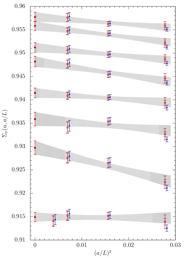
Figure 1: Continuum extrapolations of $\Sigma_{\rm\scriptscriptstyle P}$ at fixed value of $u$ in the high-energy region. Open blue triangles correspond to $\Sigma_{\rm\scriptscriptstyle P}$, while open red circles correspond to $\Sigma_{\rm\scriptscriptstyle P}^{\rm\scriptscriptstyle I}$; the latter include the systematic uncertainty discussed in the text, visible as a double error bar only in the $L/a=6$ data. The extrapolations shown (filled red circles and grey bands) are those for $\Sigma_{\rm\scriptscriptstyle P}^{\rm\scriptscriptstyle I}$.

Our second procedure, labelled as $\sigma_{\rm\scriptscriptstyle P}$:global, is a global analysis of our data, in which the $\Sigma_{\rm\scriptscriptstyle P}^{\rm\scriptscriptstyle I}(u,a/L)$-extrapolation is performed with respect to both variables $u$ and $a/L$. We extrapolate our dataset using Eq. (3.42), with $\sigma_{\rm\scriptscriptstyle P}(u)$ expanded according to Eq. (3.43), and $\rho_{\rm\scriptscriptstyle P}(u)$ expanded according to

$$\rho_{\rm\scriptscriptstyle P}(u)=\sum_{n=2}^{n_{\rho}}\rho_{n}u^{n}\,.$$ (3.46)

Since our data have been corrected for cutoff effects up to one-loop, we consistently drop terms $u^{0}$ and $u^{1}$ from the above polynomial. This series expansion is truncated at either $n_{\rho}=2$ or $n_{\rho}=3$. The series expansion of Eq. (3.43), is truncated either at $n_{s}=4$ or $n_{s}=5$. Again, the choice of $c_{2}$ is labelled as FITA (if it is left as a free fit parameter) or FITB (if $c_{2}=s_{2}$). Once $\sigma_{\rm\scriptscriptstyle P}(u)$ has been obtained from the global extrapolation, the RG running is determined from Eq. (3.45), just like in procedure $\sigma_{\rm\scriptscriptstyle P}$:u-by-u.

The third procedure, labelled as $\tau$:u-by-u, starts off just like $\sigma_{\rm\scriptscriptstyle P}$:u-by-u: at constant $u$, we fit the datapoints $\Sigma_{\rm\scriptscriptstyle P}^{\rm\scriptscriptstyle I}(u,a/L)$ with Eq. (3.42), obtaining $\sigma_{\rm\scriptscriptstyle P}(u)$. Then the continuum values $\sigma_{\rm\scriptscriptstyle P}(u)$ are fit with Eq. (2.9b), where in the integrand we use the results of Sect. 2 for the $\beta$ function (cf. Eqs. (2.34-2.36)) and the polynomial ansatz

$$\tau(x)=-x^{2}\sum_{n=0}^{n_{s}}t_{n}x^{2n}$$ (3.47)

for the quark mass anomalous dimension. We fix the two leading coefficients to the perturbative asymptotic predictions $t_{0}=d_{0}\approx 0.05066$ and $t_{1}=d_{1}\approx 0.002969$ (this is labelled as FITB). The coefficients $t_{n>1}$ are free fit parameters and the series is truncated at $n_{s}=2,\ldots,5$.

Having thus obtained an estimate for the anomalous dimension $\tau(u)$, we arrive at another determination of the renormalised-mass ratios, using the expression

$$\begin{split}R^{(k)}&\equiv\frac{\kern 2.0pt\overline{\kern-1.0ptm\kern-1.0pt}\kern 1.0pt(2^{k}\mu_{0})}{\kern 2.0pt\overline{\kern-1.0ptm\kern-1.0pt}\kern 1.0pt(\mu_{0}/2)}=\exp\left\{-\int_{\sqrt{u_{k}}}^{\sqrt{u_{-1}}}{\rm d}x\,\frac{\tau(x)}{\beta(x)}\right\}\,,\end{split}$$ (3.48)

with the couplings determined through Eq. (3.44).

Our fourth procedure, labelled as $\tau$:global, consists in performing the continuum extrapolation of $\Sigma_{\rm\scriptscriptstyle P}(u,a/L)$ and the determination of the anomalous dimension $\tau(u)$ simultaneously. Once more, $\Sigma_{\rm\scriptscriptstyle P}(u,a/L)$ is treated as a function of two variables. This approach is based on the relation

$$\ln\left(\Sigma_{\rm\scriptscriptstyle P}^{\rm\scriptscriptstyle I}(u,a/L)-\rho_{\rm\scriptscriptstyle P}(u)\left(\frac{a}{L}\right)^{2}\right)=-\int_{\sqrt{u}}^{\sqrt{\sigma(u)}}{\rm d}x\,\frac{\tau(x)}{\beta(x)}\,.$$ (3.49)

with $\rho_{\rm\scriptscriptstyle P}(u)$ and $\tau(u)$ parameterised by the polynomial ansätze (3.46) and (3.47) respectively, and the $\beta$ function being again provided by Eqs. (2.34-2.36). In practice the $\rho_{\rm\scriptscriptstyle P}(u)$-series is truncated at $n_{\rho}=2,3$. Again we account for the one-loop correction of our data for cutoff effects by consistently dropping terms $u^{0}$ and $u^{1}$ from the $\rho_{\rm\scriptscriptstyle P}(u)$-polynomial. For the $\tau$-series, we always fix the leading universal coefficient to the perturbative asymptotic prediction $t_{0}=d_{0}\approx 0.05066$, while we either leave the rest of the coefficients to be determined by the fit (labelled FITA), or fix the ${\rm O}(x^{4})$ coefficient to the perturbative prediction $t_{1}=d_{1}\approx 0.002969$ (labelled FITB).

Like in the previous $\tau$:u-by-u procedure, having obtained an estimate for the anomalous dimension $\tau(u)$, we again arrive at an expression for the renormalised-mass ratios using Eq. (3.48).

The main advantage of the two u-by-u analyses is that one has full control over the continuum extrapolations, since they are performed independently of the determination of the anomalous dimension. The disadvantage is that having to fit, for most $u$-values, three datapoints with the two-parameter function (3.42), we are forced to include our $L/a=6$ results, which are affected by the largest discretisation errors. As far as the two global analyses are concerned, they have two advantages. First, one can choose not to include the coarser lattice data points, i.e., one can fit only to the data with $L/a>6$. This provides an extra handle on the control of cutoff effects. Second, slight mistunings in the value of the coupling $u$ can be incorporated by the fit.

In order to have a meaningful quantitative comparison of the four procedures, we display in Table 7 results for $R^{(k)}$, obtained from all four methods and for a variety of fit ansätze. In general, the agreement is good, though it is clear that the fit quality improves when the data with $L/a=6$ are discarded. Fits for $\tau$ that do not use the known value for $t_{1}$ tend to have larger errors, as expected, since the asymptotic perturbative behavior is not constrained by the known analytic results. We therefore focus on FITB. Concerning fits from procedures $\sigma_{\rm\scriptscriptstyle P}$:u-by-u and $\sigma_{\rm\scriptscriptstyle P}$:global, the parameterisation with $n_{s}=5$ tends to provide a better description of our data. Anyway, the key point is that the analysis coming from the recursion of the step scaling functions is in good agreement with that coming from a direct determination of the anomalous dimension.

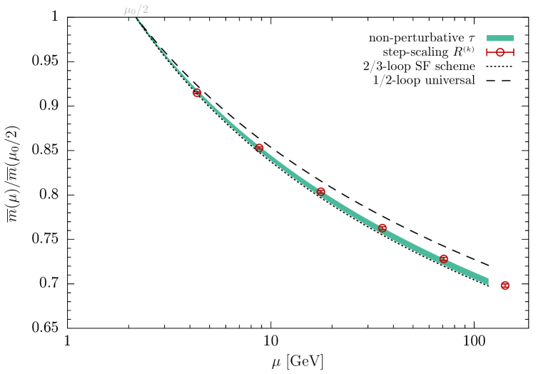
Figure 2: RG evolution factor towards high energies from the lowest energy scale $\mu_{0}/2$ reached with the ${\rm SF}$ scheme, given by the ratio $\kern 2.0pt\overline{\kern-1.0ptm\kern-1.0pt}\kern 1.0pt(\mu)/\kern 2.0pt\overline{\kern-1.0ptm\kern-1.0pt}\kern 1.0pt(\mu_{0}/2)$. The green band is the result from our preferred determination of the anomalous dimension, Eq. (3.50), in the region covered by our data, while the red points are the values of $R^{(k)}$ obtained from the step scaling in factors of $2$ based on $\sigma_{\rm\scriptscriptstyle P}$. For the latter we have used the u-by-u FITB results with $n_{s}=5$ from Table 7. The scale setting to obtain $\mu$ in physical units uses $\mu_{0}\approx 4\,{\rm GeV}$, obtained from $\Lambda_{\rm\scriptscriptstyle QCD}$ in [32]. Perturbative predictions at different orders are also shown for comparison.

Based on this discussion, we quote as our preferred result the determination of $\tau$ from a global FITB without the $L/a=6$ data, and $n_{s}=n_{\rho}=2$. We refer to this determination as FITB* in the following. The result for the anomalous dimension at high energies is thus given by

$$\tau(g)=-g^{2}\sum_{n=0}^{2}t_{n}g^{2n}\,;$$

$$t_{0}=\frac{8}{(4\pi)^{2}}\,,\qquad t_{1}=0.002969\,,\qquad t_{2}=-0.00009(26)\,,$$ (3.50)

and is illustrated in Fig. 3. We stress that this result comes from a conservative approach, since we drop the $L/a=6$ data, and the statistical error of the points is increased by the value of the one-loop prediction for cutoff effects. To illustrate the good agreement of the various determinations of the running mass, Fig. 2 illustrates the comparison between our preferred fit for the anomalous dimension and the values obtained from the recursion based on $\sigma_{\rm\scriptscriptstyle P}$, demonstrating the excellent level of agreement between otherwise fairly different analyses, as well as the comparison with perturbative predictions.

3.3 Connection to RGI masses

In order to make the connection with RGI masses, as spelled out in our strategy in Sec. 2, we could apply NLO perturbation theory directly at an energy scale $\mu_{\rm\scriptscriptstyle pt}$ at the higher end of our data-covered range — e.g., the one defined by $\kern 1.0pt\overline{\kern-1.0ptg\kern 0.0pt}\kern 1.0pt_{\rm\scriptscriptstyle SF}^{2}(\mu_{\rm\scriptscriptstyle pt})=1.11$ — to compute $M/\kern 2.0pt\overline{\kern-1.0ptm\kern-1.0pt}\kern 1.0pt(\mu_{\rm\scriptscriptstyle pt})$, and multiply it with the non-perturbative result for $\kern 2.0pt\overline{\kern-1.0ptm\kern-1.0pt}\kern 1.0pt(\mu_{\rm\scriptscriptstyle pt})/\kern 2.0pt\overline{\kern-1.0ptm\kern-1.0pt}\kern 1.0pt(\mu_{0}/2)$. We however observe that the perturbative description of the running above $\mu_{\rm\scriptscriptstyle pt}$ can be constrained by employing our non-perturbatively determined form of $\tau$, which at very small values of the coupling agrees with the asymptotic perturbative expression by construction. It is thus possible to directly compute the quantity

$$\frac{M}{\kern 2.0pt\overline{\kern-1.0ptm\kern-1.0pt}\kern 1.0pt(\mu_{0}/2)} = [2b_{0}\kern 1.0pt\overline{\kern-1.0ptg\kern 0.0pt}\kern 1.0pt_{\rm\scriptscriptstyle SF}^{2}(\mu_{0}/2)]^{-d_{0}/2b_{0}}\exp\left\{-\int_{0}^{\kern 1.0pt\overline{\kern-1.0ptg\kern 0.0pt}\kern 1.0pt_{\rm\scriptscriptstyle SF}(\mu_{0}/2)}\kern-15.0pt{\rm d}x\left[\frac{\tau(x)}{\beta(x)}-\frac{d_{0}}{b_{0}x}\right]\right\}\,,$$ (3.51)

using as input the $\tau$ function from different fits, in order to assess the systematic uncertainty of the procedure.

Type	$n_{s}$	$n_{\rho}$	$[L/a]_{\rm min}$	$M/m(\mu_{0}/2)$	$\chi^{2}/{\rm dof}$
FITB	2	2	6	1.7577(77)	18/23
FITB*	2	2	8	1.7505(89)	12/15
FITB	3	2	6	1.7580(80)	18/22
FITB	3	2	8	1.7500(97)	12/14

Table 2: Various fits of the anomalous dimension and results for $M/\kern 2.0pt\overline{\kern-1.0ptm\kern-1.0pt}\kern 1.0pt(\mu_{0}/2)$, see section 3.3.

The result of this exercise for a selection of global fits for $\tau$, both with and without the $L/a=6$ data, is provided in Table 2. The agreement among different parameterisations of the anomalous dimension is very good. The value coming from our preferred fit is

$$\frac{M}{\kern 2.0pt\overline{\kern-1.0ptm\kern-1.0pt}\kern 1.0pt(\mu_{0}/2)}=1.7505(89)\,.$$ (3.52)

This is our final result coming from the high-energy region, bearing a $0.5\%$ error. As stressed above, our error estimates can be deemed conservative; an extra-conservative error estimate could be obtained by adding in quadrature the maximum spread of central values in Table 2, which would yield a $0.7\%$ final uncertainty. We however consider the latter an overestimate, and stick to Eq. (3.52) as our preferred value.

4 Running in the low-energy region

As already explained, at energies $\mu<\mu_{0}/2$ it is convenient to change to the GF scheme. The objective of the low-energy running is to compute the ratio $\kern 2.0pt\overline{\kern-1.0ptm\kern-1.0pt}\kern 1.0pt(\mu_{0}/2)/\kern 2.0pt\overline{\kern-1.0ptm\kern-1.0pt}\kern 1.0pt(\mu_{\rm\scriptscriptstyle had})$, that, together with the ratio $M/\kern 2.0pt\overline{\kern-1.0ptm\kern-1.0pt}\kern 1.0pt(\mu_{0}/2)$ of eq. (3.51), will provide the total running factor.

We have again determined the step scaling function $\Sigma_{\rm\scriptscriptstyle P}$ of Eq. (2.14) at three different values of the lattice spacing, now using lattices of size $T/a=L/a=8,12,16$, and double lattices of size $L/a=16,24,32$. The bare parameters are chosen so that $u_{\rm\scriptscriptstyle GF}$ is approximately equal to one of the seven values

$$\{2.12,2.39,2.73,3.20,3.86,4.49,5.29\}\,.$$ (4.53)

Note that the lattice sizes are larger than in the high-energy region. This allows to better tackle cutoff effects, which are expected to be larger because of the stronger coupling, and the larger scaling violations exhibited by $u_{\rm\scriptscriptstyle GF}$ with respect to $u_{\rm\scriptscriptstyle SF}$ [61, 29, 31]. Simulations have been carried out using a tree-level Symanzik improved (Lüscher-Weisz) gauge action [74], and an $\mbox{O}(a)$-improved fermion action [68] with the non-perturbative value of the improvement coefficient $c_{\rm sw}$ [75] and one-loop values of the coefficients $c_{\rm t},\tilde{c}_{\rm t}$ for boundary improvement counterterms [76, 77, 66]. The chiral point is set using the same strategy as before, cf. Section 3. In contrast to the high-energy region, here the coupling constant $\kern 1.0pt\overline{\kern-1.0ptg\kern 0.0pt}\kern 1.0pt_{\rm\scriptscriptstyle GF}^{2}$ and $Z_{\rm\scriptscriptstyle P}$ are measured on the same ensembles, and hereafter we take the resulting correlations into account in our analysis. As discussed in Section 2, computations are carried out at fixed topological charge $Q=0$. The main motivation for this is the onset of topological freezing [78] within the range of bare coupling values covered by our simulations; setting $Q=0$ allows to circumvent the large computational cost required to allow the charge to fluctuate in the ensembles involved. The projection is implemented as proposed in [79, 31]. In practice, this is only an issue for the finest ensembles at the largest values of $u_{\rm\scriptscriptstyle GF}$ — for $u_{\rm\scriptscriptstyle GF}\lesssim 4$ no configurations with nonzero charge have been observed in simulations where the projection is not implemented.

The results of our simulations are summarised in Table 8. Note that, contrary to the high-energy region, here the value of $u_{\rm\scriptscriptstyle GF}$ is not exactly tuned to a constant value for different $L/a$. In practice, the slight mistuning is not visible when extrapolating our data to the continuum, but our data set simply begs to be analysed using the global approach described in Section 3. This approach only requires to have pairs of lattices of sizes $L/a$ and $2L/a$ simulated at the same values of the bare parameters.

Moreover, there is no guarantee that when computing $\kern 2.0pt\overline{\kern-1.0ptm\kern-1.0pt}\kern 1.0pt(\mu_{0}/2)/\kern 2.0pt\overline{\kern-1.0ptm\kern-1.0pt}\kern 1.0pt(\mu_{\rm\scriptscriptstyle had})$ the scale factor $\mu_{\rm\scriptscriptstyle had}/\mu_{0}$ is an integer power of two. This speaks in favour of performing the analysis using the anomalous dimension. As in the previous section, we will use the available information on the $\beta$ function, eq. (2.36). We will parameterise the ratio of RG functions as

$$f(x)=\frac{\tau(x)}{\beta(x)}=\frac{1}{x}\sum_{n=0}^{n_{r}}f_{n}x^{2n}\,,$$ (4.54)

and determine the fit parameters $f_{n}$ via a fit to the usual relation

$$\log\left[\Sigma_{\rm\scriptscriptstyle P}(u,a/L)-\rho(u)(a/L)^{2}\right]=-\int_{\sqrt{u}}^{\sqrt{\sigma(u)}}{\rm d}x\,f(x)\,.$$ (4.55)

Once more, $\rho(u)$ describes the cutoff effects in $\sigma_{\rm\scriptscriptstyle P}(u)$. When the fit parameters $f_{n}$ are determined, we can reconstruct the anomalous dimension thanks to the relation

$$f(\kern 1.0pt\overline{\kern-1.0ptg\kern 0.0pt}\kern 1.0pt)=\frac{\tau(\kern 1.0pt\overline{\kern-1.0ptg\kern 0.0pt}\kern 1.0pt)}{\beta(\kern 1.0pt\overline{\kern-1.0ptg\kern 0.0pt}\kern 1.0pt)}\quad\Longrightarrow\quad\tau(\kern 1.0pt\overline{\kern-1.0ptg\kern 0.0pt}\kern 1.0pt)=-\kern 1.0pt\overline{\kern-1.0ptg\kern 0.0pt}\kern 1.0pt^{2}\frac{\sum_{n=0}^{n_{r}}f_{n}\kern 1.0pt\overline{\kern-1.0ptg\kern 0.0pt}\kern 1.0pt^{2n}}{\sum_{k=0}^{k_{t}}p_{k}\kern 1.0pt\overline{\kern-1.0ptg\kern 0.0pt}\kern 1.0pt^{2k}}\,.$$ (4.56)

Recall that the parameters $p_{n}$ define our $\beta$ function in Eq. (2.36).

	$n_{r}=2$		$n_{r}=3$
$\rho(u)$	$\kern 2.0pt\overline{\kern-1.0ptm\kern-1.0pt}\kern 1.0pt(\mu_{0}/2)/\kern 2.0pt\overline{\kern-1.0ptm\kern-1.0pt}\kern 1.0pt(\mu_{\rm had})$	$\chi^{2}/{\rm dof}$	$\kern 2.0pt\overline{\kern-1.0ptm\kern-1.0pt}\kern 1.0pt(\mu_{0}/2)/\kern 2.0pt\overline{\kern-1.0ptm\kern-1.0pt}\kern 1.0pt(\mu_{\rm had})$	$\chi^{2}/{\rm dof}$
$\rho_{1}u+\rho_{2}u^{2}$	0.5245(41)	11/16	0.5250(42)	11/15
$\rho_{0}+\rho_{1}u+\rho_{2}u^{2}$	0.5222(43)	9.5/15	0.5226(43)	6.5/14
$\rho_{1}u+\rho_{2}u^{2}+\rho_{3}u^{3}$	0.5201(45)	7.4/14	0.5208(45)	6.0/13

Table 3: Results for the running factor $\kern 2.0pt\overline{\kern-1.0ptm\kern-1.0pt}\kern 1.0pt(\mu_{0}/2)/\kern 2.0pt\overline{\kern-1.0ptm\kern-1.0pt}\kern 1.0pt(\mu_{\rm had})$

We have tried different ansätze, and as long as $n_{r}>1$ one gets a good description of the data. The largest systematic dependence in our results comes from the functional form of $\rho(u)$. Various simple polynomials have been used, as described in Table 3. As the reader can check, all fit ansätze produce results for $\kern 2.0pt\overline{\kern-1.0ptm\kern-1.0pt}\kern 1.0pt(\mu_{0}/2)/\kern 2.0pt\overline{\kern-1.0ptm\kern-1.0pt}\kern 1.0pt(\mu_{\rm had})$ that agree within one sigma. As final result we choose the fit with $n_{r}=3$ and $\rho(u)=\rho_{0}+\rho_{1}u+\rho_{2}u^{2}$, which has the best $\chi^{2}/{\rm dof}$, and yields

$$\kern 2.0pt\overline{\kern-1.0ptm\kern-1.0pt}\kern 1.0pt(\mu_{0}/2)/\kern 2.0pt\overline{\kern-1.0ptm\kern-1.0pt}\kern 1.0pt(\mu_{\rm had})=0.5226(43)\,.$$ (4.57)

The corresponding $\tau(x)$ function is obtained from Eq. (4.56) by using the coefficients

$$f_{0}=1.28493\,,~{}f_{1}=-0.292465\,,~{}f_{2}=0.0606401\,,~{}f_{3}=-0.00291921$$ (4.58)

together with the known coefficients for the $\beta$ function in Eq. (2.36). The covariance between the $f_{n}$ parameters reads

$$\begin{split}{\rm cov}(f_{i},f_{j})=&\left({\footnotesize\begin{array}[]{cccc}\phantom{+}2.33798\times 10^{-2}&-1.47011\times 10^{-2}&\phantom{+}2.81966\times 10^{-3}&-1.66404\times 10^{-4}\\ -1.47011\times 10^{-2}&\phantom{+}9.54563\times 10^{-3}&-1.87752\times 10^{-3}&\phantom{+}1.12962\times 10^{-4}\\ \phantom{+}2.81966\times 10^{-3}&-1.87752\times 10^{-3}&\phantom{+}3.78680\times 10^{-4}&-2.32927\times 10^{-5}\\ -1.66404\times 10^{-4}&\phantom{+}1.12962\times 10^{-4}&-2.32927\times 10^{-5}&\phantom{+}1.46553\times 10^{-6}\\ \end{array}}\right)\,.\end{split}$$ (4.59)

Finally, the covariance between the $p_{i}$ and the $f_{j}$ parameters is given by

$$\begin{split}{\rm cov}(f_{i},p_{j})=&\left({\footnotesize\begin{array}[]{ccc}-3.83814\times 10^{-2}&\phantom{+}1.25288\times 10^{-2}&-8.87274\times 10^{-4}\\ \phantom{+}1.58985\times 10^{-2}&-5.23410\times 10^{-3}&\phantom{+}3.68003\times 10^{-4}\\ -1.85736\times 10^{-3}&\phantom{+}5.57473\times 10^{-4}&-3.58668\times 10^{-5}\\ \phantom{+}6.39488\times 10^{-5}&-1.45530\times 10^{-5}&\phantom{+}5.96571\times 10^{-7}\\ \end{array}}\right)\,.\end{split}$$ (4.60)

The functional form of the anomalous dimension with its uncertainty can thus be easily reproduced, and is shown in Fig. 3. Together with the result for $\tau$ in the high-energy region discussed in Section 3, and the result in Eq. (3.52), one has then all the ingredients needed to reconstruct the scale dependence of light quark masses in the full energy range relevant to SM physics, as shown in Fig. 4.

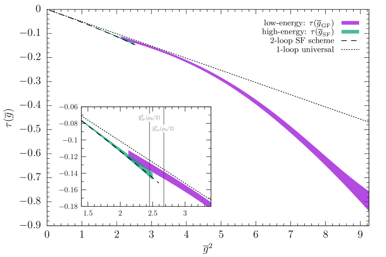
Figure 3: Non-perturbative mass anomalous dimension in the ${\rm SF}$ (green) and ${\rm GF}$ (purple) regions. Perturbative predictions at the highest available orders are also shown for comparison.

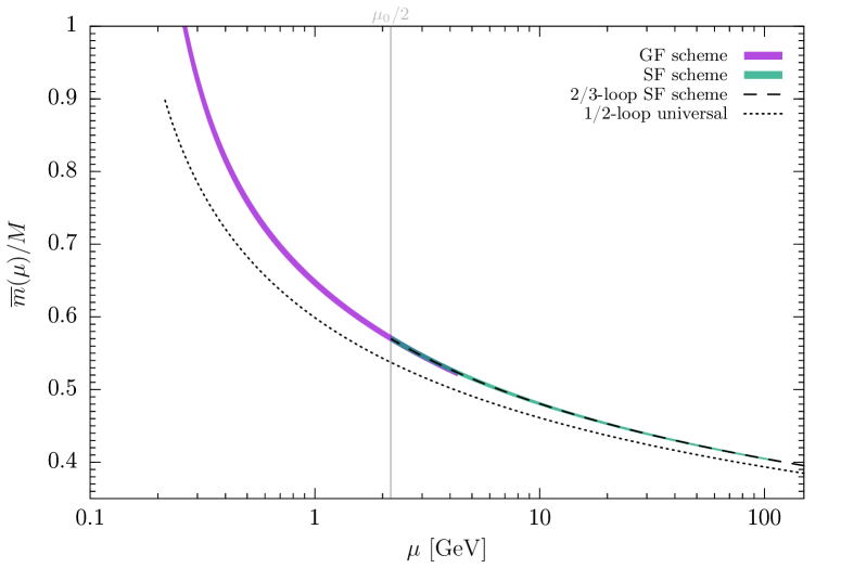
Figure 4: Non-perturbative running of light quark masses as a function of the energy scale, down to our hadronic matching scale. The value of $\mu$ in physical units has been obtained by using the result for $\Lambda_{\rm\scriptscriptstyle QCD}$ in [32]. Perturbative predictions at different orders are also shown for comparison.

Let us end this section by pointing out that the coefficient $f_{0}=1.2(2)$ is compatible within $1.5\sigma$ with the one-loop perturbative prediction $d_{0}/b_{0}$. This is quite surprising, especially taking into account that the $\beta$ function is not compatible with the one-loop functional form with coefficient $b_{0}$. This in turn means that also the anomalous dimension $\tau$ is poorly approximated by one-loop perturbation theory. One is thus driven to conclude that the agreement of $f_{0}$ with LO perturbation theory is only apparent.

5 Hadronic matching and total renormalisation factor

The last step in our strategy requires the computation of the PCAC quark mass renormalisation factors $Z_{\rm m}$ at hadronic scales, cf. Eq. (2.38). The latter can be written as

$$Z_{\rm m}(g_{0}^{2},a\mu_{\rm\scriptscriptstyle had})=\frac{Z_{\rm\scriptscriptstyle A}(g_{0}^{2})}{Z_{\rm\scriptscriptstyle P}(g_{0}^{2},a\mu_{\rm\scriptscriptstyle had})}\,$$ (5.61)

Since the values of the axial current normalisation $Z_{\rm\scriptscriptstyle A}$ are available from a separate computation [81, 82, 83] (in particular we use the precise values obtained thanks to the chirally rotated SF setup [84, 85, 86]), in order to obtain $Z_{\rm m}$ we just need to determine $Z_{\rm\scriptscriptstyle P}(g_{0}^{2},a\mu_{\rm\scriptscriptstyle had})$ at a fixed value of $\mu_{\rm\scriptscriptstyle had}$ for changing bare coupling $g_{0}^{2}$. The values of $g_{0}^{2}$ have to be in the range used in large-volume simulations; for practical purposes, we will thus target the interval $\beta=6/g_{0}^{2}\in[3.40,3.85]$ currently covered by CLS ensembles [47, 87].

Our strategy proceeds as follows. We first choose a value of $u_{\rm\scriptscriptstyle had}=\kern 1.0pt\overline{\kern-1.0ptg\kern 0.0pt}\kern 1.0pt_{\rm\scriptscriptstyle GF}^{2}(\mu_{\rm\scriptscriptstyle had})$ such that the relevant $g_{0}^{2}$ range is covered using accessible values of $L/a$. The precise value of $u_{\rm\scriptscriptstyle had}$ is fixed by simulating at one of the finest lattices. Finally, other lattice sizes are simulated, such that we can obtain an interpolating formula for $Z_{\rm\scriptscriptstyle P}(g_{0}^{2},a\mu_{\rm\scriptscriptstyle had})$ as a function of $g_{0}^{2}$ along the line of constant physics fixed by $u_{\rm\scriptscriptstyle had}$. We have set $u_{\rm\scriptscriptstyle had}=9.25$, fixed by simulating on an $L/a=20$ lattice at $\beta=3.79$. Lattice sizes $L/a=16,12,10$ have then been used at smaller $\beta$, and two $L/a=24$ lattices have been added so that the finest $\beta=3.85$ point can be safely interpolated. Using the results in [32], this value of $u_{\rm\scriptscriptstyle had}$ corresponds to an energy scale $\mu_{\rm\scriptscriptstyle had}=233(8)~{}{\rm MeV}$.

Our simulation results are summarised in Table 4. Deviations from the target values of $u_{\rm\scriptscriptstyle had}$ induce a small but visible effect on $Z_{\rm\scriptscriptstyle P}$. The measured values of the PCAC mass are often beyond our tolerance $|Lm|\lesssim 0.001$ (cf. App. A), especially for the smaller lattice sizes. This is a consequence of the fact that the interpolating formula for $\kappa_{\rm c}$ as a function of $g_{0}^{2}$ loses precision for $L/a=10$, and of the small cutoff effect induced by computing at zero topological charge (which is part of our renormalisation condition). Note that the values of $Z_{\rm\scriptscriptstyle P}$ that enter the fit function are never further away than two standard deviations from the value on the lattice that defines the line of constant physics. The fitted dependences on $g_{0}^{2}$, $u_{\rm\scriptscriptstyle GF}$, and $Lm$ are thus very mild.

$L/a$	$\beta$	$\kappa$	$u_{\rm\scriptscriptstyle GF}$	$Lm$	$Z_{\rm\scriptscriptstyle P}(g_{0}^{2},L/a)$	# cfg
$10$	$3.4000$	$0.1368040500$	$9.282(39)$	$-0.0221(31)$	$0.3484(11)$	$2489$
$10$	$3.4110$	$0.1367650000$	$9.290(32)$	$+0.0189(23)$	$0.3526(10)$	$4624$
$12$	$3.4800$	$0.1370389800$	$9.406(41)$	$-0.0115(32)$	$0.3417(14)$	$1828$
$12$	$3.4880$	$0.1370210000$	$9.393(43)$	$+0.0035(23)$	$0.3430(15)$	$2667$
$12$	$3.4970$	$0.1370629900$	$9.118(54)$	$-0.0102(32)$	$0.3487(18)$	$1491$
$16$	$3.6490$	$0.1371576500$	$9.423(39)$	$-0.0024(17)$	$0.3430(19)$	$4560$
$16$	$3.6576$	$0.1371541300$	$9.186(50)$	$-0.0039(18)$	$0.3492(17)$	$3079$
$16$	$3.6710$	$0.1371475600$	$9.045(91)$	$+0.0009(26)$	$0.3526(28)$	$1553$
$20$	$3.7900$	$0.1370480000$	$9.251(54)$	$-0.0008(11)$	$0.3508(22)$	$4133$
$24$	$3.8934$	$0.1368944446$	$9.382(56)$	$-0.0001(11)$	$0.3474(20)$	$4709$
$24$	$3.9122$	$0.1368621644$	$9.132(51)$	$+0.0001(7)$	$0.3543(22)$	$5086$

Table 4: Results for $Z_{\rm\scriptscriptstyle P}$ in the ${\rm GF}$ scheme, used to determine quark mass renormalization constants at $u_{\rm\scriptscriptstyle had}=9.25$. Alongside the values of $u_{\rm\scriptscriptstyle GF}$ and $Z_{\rm\scriptscriptstyle P}$, we also quote the value of the PCAC mass $m$ in units of the physical lattice length, and the statistics for each ensemble.

The measured values of $Z_{\rm\scriptscriptstyle P}$ are fitted to a function of the form

$$\begin{split}Z_{\rm\scriptscriptstyle P}(g_{0}^{2},u_{\rm\scriptscriptstyle GF},Lm)&=Z_{\rm\scriptscriptstyle P}^{\rm\scriptscriptstyle had}(g_{0}^{2})+t_{10}\,(u_{\rm\scriptscriptstyle GF}-u_{\rm\scriptscriptstyle had})+t_{20}\,(u_{\rm\scriptscriptstyle GF}-u_{\rm\scriptscriptstyle had})^{2}\\ &\qquad\qquad\quad+t_{01}\,Lm+t_{11}\,(u_{\rm\scriptscriptstyle GF}-u_{\rm\scriptscriptstyle had})Lm\,,\\ Z_{\rm\scriptscriptstyle P}^{\rm\scriptscriptstyle had}(g_{0}^{2})&=z_{0}+z_{1}(\beta-\beta_{0})+z_{2}(\beta-\beta_{0})^{2}\,,\end{split}$$ (5.62)

where $u_{\rm\scriptscriptstyle had}=9.25$ and $\beta_{0}=3.79$. The terms with coefficients $t_{ij}$ parameterise the small deviations from the intended line of constant physics described above, while $Z_{\rm\scriptscriptstyle P}^{\rm\scriptscriptstyle had}$ is the interpolating function we are interested in. Note that the ensembles are fully uncorrelated among them, but within each ensemble the values of $u_{\rm\scriptscriptstyle GF}$, $Lm$, and $Z_{\rm\scriptscriptstyle P}$ are correlated, and we take this into account in the fit procedure. We have performed fits setting to zero various subsets of $t_{ij}$ coefficients; we quote as our preferred result the one with $t_{20}=t_{11}=0$, for which $\chi^{2}/{\rm dof}=4.43/6$, and the coefficients for the interpolating function $Z_{\rm\scriptscriptstyle P}^{\rm\scriptscriptstyle had}$ read

$$z_{0}=0.348629\,,\quad z_{1}=0.020921\,,\quad z_{2}=0.070613\,,$$ (5.63a)

with covariance matrix

$${\rm cov}(z_{i},z_{j})=\left(\begin{array}[]{rrr}0.375369\times 10^{-6}&0.429197\times 10^{-6}&-0.186896\times 10^{-5}\\ 0.429197\times 10^{-6}&0.268393\times 10^{-4}&0.686776\times 10^{-4}\\ -0.186896\times 10^{-5}&0.686776\times 10^{-4}&0.212386\times 10^{-3}\\ \end{array}\right)\,.$$ (5.63b)

The typical precision of the values of $Z_{\rm\scriptscriptstyle P}$ extracted from the interpolating function is thus at the few permille level. The fit is illustrated in Fig. 5.

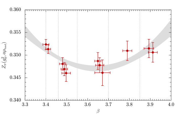
Figure 5: Projection on the $(\beta,Z_{\rm\scriptscriptstyle P})$ plane of the fit (grey band) to the results for $Z_{\rm\scriptscriptstyle P}$ at the hadronic matching point $u_{\rm\scriptscriptstyle had}=9.25$ (filled red points). The data points have been shifted to the target value of $u_{\rm\scriptscriptstyle GF}$ and $Lm=0$ using the fit function. Horizontal error bars have been assigned to reflect the uncertainties coming from the value of $u_{\rm\scriptscriptstyle GF}$ for each point, by defining $\Delta g_{0}^{2}/g_{0}^{2}=\Delta u_{\rm\scriptscriptstyle GF}/u_{\rm\scriptscriptstyle GF}$. Vertical dashed lines correspond to the $\beta$ values of CLS ensembles.

Now we can finally assemble the various factors entering Eqs. (2.37,2.38). Using the results in Sec. 4 we can compute the running $\kern 2.0pt\overline{\kern-1.0ptm\kern-1.0pt}\kern 1.0pt(\mu_{0}/2)/\kern 2.0pt\overline{\kern-1.0ptm\kern-1.0pt}\kern 1.0pt(\mu_{\rm\scriptscriptstyle had})$ between the scheme-switching scale and hadronic matching scale, and multiply it by the value of $M/\kern 2.0pt\overline{\kern-1.0ptm\kern-1.0pt}\kern 1.0pt(\mu_{0}/2)$ given in Eq. (3.52). Combining the errors in quadrature, we obtain

$$\frac{M}{\kern 2.0pt\overline{\kern-1.0ptm\kern-1.0pt}\kern 1.0pt(\mu_{\rm\scriptscriptstyle had})}=0.9148(88)\,,$$ (5.64)

which has a $0.96$% precision; recall $\mu_{\rm\scriptscriptstyle had}=233(8)~{}{\rm MeV}$. It is important to stress that Eq. (5.64) holds in the continuum, i.e., it is independent of any detail of the lattice computation. We can then take our interpolating formula for $Z_{\rm\scriptscriptstyle P}$ and the known results for $Z_{\rm\scriptscriptstyle A}$, and build the total factor $Z_{\rm\scriptscriptstyle M}$ that relates RGI masses to bare PCAC masses computed with a non-perturbatively $\mbox{O}(a)$-improved fermion action and a tree-level Symanzik improved gauge action,

$$Z_{\rm\scriptscriptstyle M}(g_{0}^{2})=\frac{M}{\kern 2.0pt\overline{\kern-1.0ptm\kern-1.0pt}\kern 1.0pt(\mu_{\rm\scriptscriptstyle had})}\frac{Z_{\rm\scriptscriptstyle A}(g_{0}^{2})}{Z_{\rm\scriptscriptstyle P}(g_{0}^{2},a\mu_{\rm\scriptscriptstyle had})}\,.$$ (5.65)

Recall that the dependence of $Z_{\rm\scriptscriptstyle M}$ on $\mu_{\rm\scriptscriptstyle had}$ has to cancel exactly, up to residual terms contributing to the cutoff effects of $Z_{\rm\scriptscriptstyle M}(g_{0}^{2})m(g_{0}^{2})$. Using as input the values of $Z_{\rm\scriptscriptstyle A}$ from the chirally rotated SF setup [84, 85, 86], we quote the interpolating function

$$\begin{gathered}Z_{\rm\scriptscriptstyle M}(g_{0}^{2})=\frac{M}{\kern 2.0pt\overline{\kern-1.0ptm\kern-1.0pt}\kern 1.0pt(\mu_{\rm\scriptscriptstyle had})}\times\left\{Z_{\rm\scriptscriptstyle M}^{(0)}+Z_{\rm\scriptscriptstyle M}^{(1)}(\beta-3.79)+Z_{\rm\scriptscriptstyle M}^{(2)}(\beta-3.79)^{2}\right\}\,;\\[4.30554pt] Z_{\rm\scriptscriptstyle M}^{(0)}=2.270073\,,\quad Z_{\rm\scriptscriptstyle M}^{(1)}=0.121644\,,\quad Z_{\rm\scriptscriptstyle M}^{(2)}=-0.464575\,,\end{gathered}$$ (5.66a)

with covariance matrix

$${\rm cov}(Z_{\rm\scriptscriptstyle M}^{(i)},Z_{\rm\scriptscriptstyle M}^{(j)})=\left(\begin{array}[]{rrr}0.164635\times 10^{-4}&0.215658\times 10^{-4}&-0.754203\times 10^{-4}\\ 0.215658\times 10^{-4}&0.121072\times 10^{-2}&0.308890\times 10^{-2}\\ -0.754203\times 10^{-4}&0.308890\times 10^{-2}&0.953843\times 10^{-2}\\ \end{array}\right)\,.$$ (5.66b)

The quoted errors only contain the uncertainties from the determination of $Z_{\rm\scriptscriptstyle A}$ and $Z_{\rm\scriptscriptstyle P}$ at the hadronic scale. As remarked in [35], the error of the total running factor $M/\kern 2.0pt\overline{\kern-1.0ptm\kern-1.0pt}\kern 1.0pt(\mu_{\rm\scriptscriptstyle had})$ in Eq. (5.64) has to be added in quadrature to the error in the final result for the RGI mass, since it only affects the continuum limit, and should not be included in the extrapolation of data for current quark masses to the continuum limit.

Finally, we note that our results can be also used to obtain renormalised quark masses when a twisted-mass QCD Wilson fermion regularisation [88] is employed in the computation. In that case the bare PCAC mass coincides with the bare twisted mass parameter, which can be renormalised with

$$Z_{\rm m}^{\rm\scriptscriptstyle tm}(g_{0}^{2},a\mu_{\rm\scriptscriptstyle had})=\frac{1}{Z_{\rm\scriptscriptstyle P}(g_{0}^{2},a\mu_{\rm\scriptscriptstyle had})}\,.$$ (5.67)

The total renormalisation factor then acquires the form

$$Z_{\rm\scriptscriptstyle M}^{\rm\scriptscriptstyle tm}(g_{0}^{2})=\frac{M}{\kern 2.0pt\overline{\kern-1.0ptm\kern-1.0pt}\kern 1.0pt(\mu_{\rm\scriptscriptstyle had})}\frac{1}{Z_{\rm\scriptscriptstyle P}(g_{0}^{2},a\mu_{\rm\scriptscriptstyle had})}\,,$$ (5.68)

and values can be obtained by directly using our interpolating formula for $Z_{\rm\scriptscriptstyle P}^{\rm\scriptscriptstyle had}$. The same comment about the combination of uncertainties as above applies. The values of $Z_{\rm\scriptscriptstyle M}$ and $Z_{\rm\scriptscriptstyle M}^{\rm\scriptscriptstyle tm}$ at the $\beta$ values of CLS ensembles are provided in Table 5.

Eqs. (5.64,5.63,5.66) are the final, and most important, results of this work. We stress once more that the result for $M/\kern 2.0pt\overline{\kern-1.0ptm\kern-1.0pt}\kern 1.0pt(\mu_{\rm\scriptscriptstyle had})$, which is by far the most computationally demanding one, holds in the continuum, and is independent of the lattice regularisation employed in its determination, as well as any other computational detail. The expressions for $Z_{\rm\scriptscriptstyle M}$ and $Z_{\rm\scriptscriptstyle M}^{\rm\scriptscriptstyle tm}$, on the other hand, depend on the action used in the computation, and hold for a non-perturbatively $\mbox{O}(a)$-improved fermion action and a tree-level Symanzik improved gauge action. Repeating the computation for a different lattice action would only require obtaining the values of $Z_{\rm\scriptscriptstyle A}$ and $Z_{\rm\scriptscriptstyle P}$ in the appropriate interval of values of $\beta$, at small computational cost.

$\beta$	$Z_{\rm\scriptscriptstyle M}$	$Z_{\rm\scriptscriptstyle M}^{\rm\scriptscriptstyle tm}$
$3.40$	1.9684(35)	2.6047(42)
$3.46$	1.9935(27)	2.6181(33)
$3.55$	2.0253(33)	2.6312(42)
$3.70$	2.0630(38)	2.6339(48)
$3.85$	2.0814(45)	2.6127(55)

Table 5: Values of the renormalisation factors $Z_{\rm\scriptscriptstyle M}$ and $Z_{\rm\scriptscriptstyle M}^{\rm\scriptscriptstyle tm}$ connecting RGI and bare PCAC masses in the standard Wilson and twisted-mass cases, respectively, at the values of $\beta$ for CLS ensembles. Recall that the quoted errors do not contain the contribution from the running factor $M/\kern 2.0pt\overline{\kern-1.0ptm\kern-1.0pt}\kern 1.0pt(\mu_{\rm\scriptscriptstyle had})$. The correlations between the errors at different $\beta$ can be readily obtained from the covariance matrices provided in Eqs. (5.66b) and (5.63b), respectively.

6 Conclusions

In this paper we have performed a fully non-perturbative, high-precision determination of the quark mass anomalous dimension in $N_{\mathrm{\scriptstyle f}}=3$ QCD, spanning from the electroweak scale to typical hadronic energies. Alongside the companion non-perturbative determination of the $\beta$ function in [29, 31], this completes the first-principles determination of the RG functions of fundamental parameters for light hadron physics. Together with the determination of the $\Lambda_{\rm\scriptscriptstyle QCD}$ parameter [32] and the forthcoming publication of renormalised quark masses [89], a full renormalisation programme of $N_{\mathrm{\scriptstyle f}}=3$ QCD will have been achieved. For the purpose of the latter computation, we have also provided a precise computation of the matching factors required to obtain renormalised quark masses from PCAC bare quark masses obtained from simulations based on CLS $N_{\mathrm{\scriptstyle f}}=2+1$ ensembles [90, 91]. The total uncertainty introduced by the matching factor to RGI quark masses is at the level of $1.1\%$.

A slight increase in this precision is achievable within the same framework. This would require however a significantly larger numerical effort, adding larger lattices and hence finer lattice spacings to the continuum limit extrapolation, and augmenting the precision for the tuning of bare parameters. One lesson from the present work is that the $1\%$ ballpark is not much above the irreducible systematic uncertainty achievable with the methodology employed. Improvements of the latter will thus be necessary to reduce the uncertainty purely due to renormalisation to the few permille level. It is important to stress that the uncertainty is completely dominated by the contribution from the non-perturbative running at low energies; another lesson from the present work is that, at this level of precision, use of perturbation theory in the few-GeV region is not necessarily satisfactory.

Apart from increasing the precision of the computation, one obvious next step is the inclusion of heavier flavours. This would ideally result in reaching sub-percent renormalisation-related uncertainties in first-principles computations of the charm and bottom quark masses, whose values play a key role in frontier studies of B- and Higgs physics. First steps in this direction, at the level of the computation of the running coupling, have already been taken [92, 93, 94].

A Systematic uncertainties in the determination of step scaling functions

A.1 Tuning of the critical mass

The tuning of the chiral point, as part of setting our lines of constant physics, is treated in detail in [66]. Briefly, a set of tuning runs at various values of $\beta$ and $\kappa$ are used to compute the PCAC mass $m$ in Eq. (2.11), and interpolate at fixed $\beta$ values for $\kappa_{\rm c}$ such that $|Lm|\leq 0.001$, with an uncertainty of at most the same order. This implies that the values of the quark mass at which the renormalisation condition in Eq. (2.26) is imposed are not exactly zero.

In order to assess the relevant systematics, we have performed dedicated simulations at the strongest coupling covered in the ${\rm SF}$ scheme, $u_{\rm\scriptscriptstyle SF}=2.0120$, for which $\Sigma_{\rm\scriptscriptstyle P}(2.0120,L/a=6)$ has been computed at the value of $\beta=6.2735$ indicated in Table 6, and four different values of $\kappa$, besides the nominal one for $\kappa_{\rm c}$ given in Table 6. This is expected to be the simulation point within the high-energy regime where systematics may have a stronger impact. The result of this exercise is shown in Fig. 6. A linear fit to the data allows to estimate the slope coefficient

$$\rho_{\kappa_{\rm c}}\equiv\frac{1}{L}\,\left.\frac{\partial\Sigma_{\rm\scriptscriptstyle P}}{\partial m}\right|_{u,L}\,,$$ (A.69)

which can then be used to assign a systematic uncertainty to $\Sigma_{\rm\scriptscriptstyle P}$ as

$$\delta_{\kappa_{\rm c}}\Sigma_{\rm\scriptscriptstyle P}=|\rho_{\kappa_{\rm c}}|{\rm tol}(Lm)\,,$$ (A.70)

where ${\rm tol}(Lm)=0.001$ is our tolerance for defining the critical point. We obtain $\rho_{\kappa_{\rm c}}=-0.15(15)$, which yields for the systematic uncertainty $\delta_{\kappa_{\rm c}}\Sigma_{\rm\scriptscriptstyle P}=0.00015(15)$.

Besides being compatible with zero within $1\sigma$, the central value is more than four times smaller than the statistical uncertainty quoted for $\Sigma_{\rm\scriptscriptstyle P}(2.0120,L/a=6)$ in Table 6. For larger lattices or smaller renormalised couplings these systematics are expected to decrease further. On the other hand, they will increase as the renormalised coupling increases, but there is no obvious reason why its relative size with respect to the statistical uncertainty will grow as well. We thus conclude that the systematic uncertainty related to the tuning to zero quark mass is negligible at the level of precision we attain in the computation of $\sigma_{\rm\scriptscriptstyle P}$.

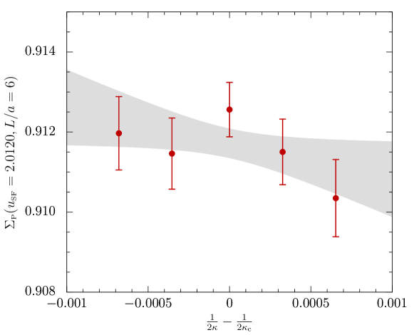
Figure 6: Variation of the SSF $\Sigma_{\rm\scriptscriptstyle P}(u_{\rm\scriptscriptstyle SF}=2.0120,L/a=6)$ with the value of the quark mass. The shadowed band is a linear fit to the data.

A.2 Tuning of the gauge coupling

Our lines of constant physics are formally defined by a nominal value of either the SF or the GF coupling, that is to be kept fixed in the lattices at which the denominator of Eq. (2.14) is computed. In practice, this is so only within some finite precision, due to two different reasons:

1. Both couplings $u_{\rm\scriptscriptstyle SF}$ or $u_{\rm\scriptscriptstyle GF}$ are computed with finite precision.

2. The ${\rm SF}$ computations of the coupling and the corresponding tuning of $\beta$ and $\kappa$ are performed using independent ensembles with respect to the ones employed for the computation of $Z_{\rm\scriptscriptstyle P}$, for reasons explained in Section 2. The resulting lines of constant physics are expected to differ by $\mbox{O}(a^{2})$ effects.

In order to assess whether the finite precision on the value of the gauge coupling has an impact on the computation of the continuum $\sigma_{\rm\scriptscriptstyle P}$, we have:

1. Repeated the continuum-limit extrapolations of $\Sigma_{\rm\scriptscriptstyle P}$ at fixed $u$, introducing a horizontal error on the value of $(a/L)^{2}$ propagated from the uncertainty on $u$ at each value of $a/L$. To that purpose one can use either the perturbative relation between $u$ and $L$, or the known non-perturbative $\beta$ functions (cf. Section 2), with little practical differences.

2. Repeated fits to the continuum-extrapolated $\sigma_{\rm\scriptscriptstyle P}$ as a function of $u$, introducing an uncertainty on $u$ that covers the spread of the computed values along that particular line of constant physics.

In either case, we have found that the impact of introducing the additional uncertainties in the final description of $\sigma_{\rm\scriptscriptstyle P}$ are completely negligible within our current level of precision. This source of systematic uncertainty is therefore ignored in our final analyses.

A.3 Perturbative values of boundary improvement coefficients

In our computation, we use perturbative values for the coefficients $c_{\rm t}$ and $\tilde{c}_{\rm t}$ that appear in Schrödinger Functional boundary $\mbox{O}(a)$ improvement counterterms, employing the highest available order for the relevant lattice action. In computations in the high-energy region, where the plaquette gauge action is used, we are able to use the corresponding two-loop value of $c_{\rm t}$ [63]. In the low-energy region, where the gauge action is tree-level Symanzik improved, the two-loop coefficient is not known, and we take the one-loop value. In the case of $\tilde{c}_{\rm t}$, we employ the one-loop value [70] throughout. Contributions from these boundary counterterms to the step scaling function $\sigma_{\rm\scriptscriptstyle P}$ start at two-loop order in perturbation theory [64], and the effects of perturbative truncation in the values of $c_{\rm t},\tilde{c}_{\rm t}$ are therefore expected to be small. A careful study of these systematic uncertainties in the SF scheme was carried out in the $N_{\mathrm{\scriptstyle f}}=0$ [35] and $N_{\mathrm{\scriptstyle f}}=2$ [36] computations. Especially in the former case, a precise statement could be made that perturbative truncation effects do not change the result for the continuum limit of $\Sigma_{\rm\scriptscriptstyle P}$ even at the largest values of the coupling. In our computation, we have performed a dedicated analysis at two values of the coupling, to check the size of the resulting effects in both the ${\rm SF}$ and ${\rm GF}$ schemes.

In order to have a quantitative handle on the effect from a shift on boundary improvement coefficients, let us formally expand $Z_{\rm\scriptscriptstyle P}$, considered as a function of, e.g., $c_{\rm t}$, in a power series of the form

$$Z_{\rm\scriptscriptstyle P}+\frac{\partial Z_{\rm\scriptscriptstyle P}}{\partial c_{\rm t}}\left(\frac{a}{L}\right)\Delta c_{\rm t}+\ldots$$ (A.71)

where $\Delta c_{\rm t}$ is the deviation with respect to the value of $c_{\rm t}$ at which $Z_{\rm\scriptscriptstyle P}$ is computed. The factor $(a/L)$ is made explicit to stress that the perturbative truncation is leaving uncancelled $\mbox{O}(a)$ terms, which we are parameterising. By simulating at a number of values of $c_{\rm t}$, keeping all other simulation parameters fixed, it is possible to estimate the slope $(\partial Z_{\rm\scriptscriptstyle P}/\partial c_{\rm t})$. A systematic uncertainty can then be assigned to $Z_{\rm\scriptscriptstyle P}$ as

$$\delta_{c_{\rm t}}Z_{\rm\scriptscriptstyle P}\approx\left|\frac{\partial Z_{\rm\scriptscriptstyle P}}{\partial c_{\rm t}}\right|\left(\frac{a}{L}\right)\delta c_{\rm t}\,,$$ (A.72)

where $\delta c_{\rm t}$ is some conservative estimate of the perturbative truncation error. Linear error propagation then yields the corresponding systematic uncertainty on $\Sigma_{\rm\scriptscriptstyle P}=Z_{\rm\scriptscriptstyle P}(2L)/Z_{\rm\scriptscriptstyle P}(L)$ as

$$\frac{\delta_{c_{\rm t}}\Sigma_{\rm\scriptscriptstyle P}}{\Sigma_{\rm\scriptscriptstyle P}}\approx\left|\frac{\partial Z_{\rm\scriptscriptstyle P}}{\partial c_{\rm t}}\left[\frac{1}{2Z_{\rm\scriptscriptstyle P}(2L)}-\frac{1}{Z_{\rm\scriptscriptstyle P}(L)}\right]\right|\left(\frac{a}{L}\right)\delta c_{\rm t}\,.$$ (A.73)

The systematic uncertainty due to the truncation in the value of $\tilde{c}_{\rm t}$ can be estimated in exactly the same way.

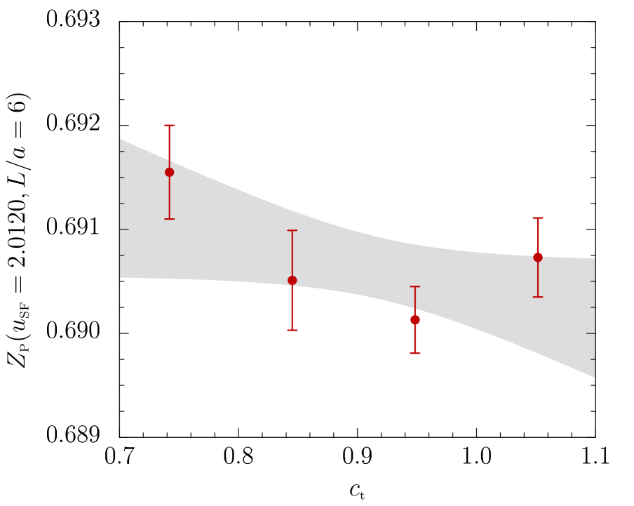
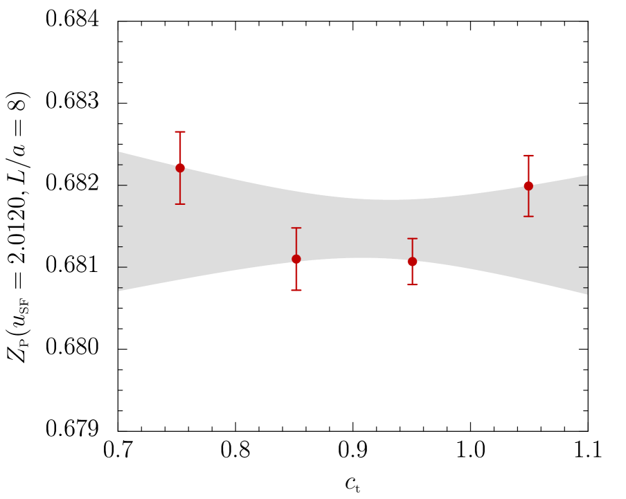
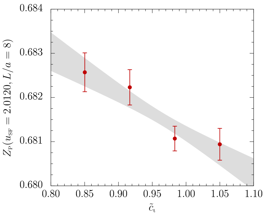
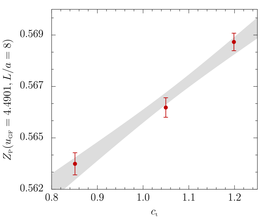
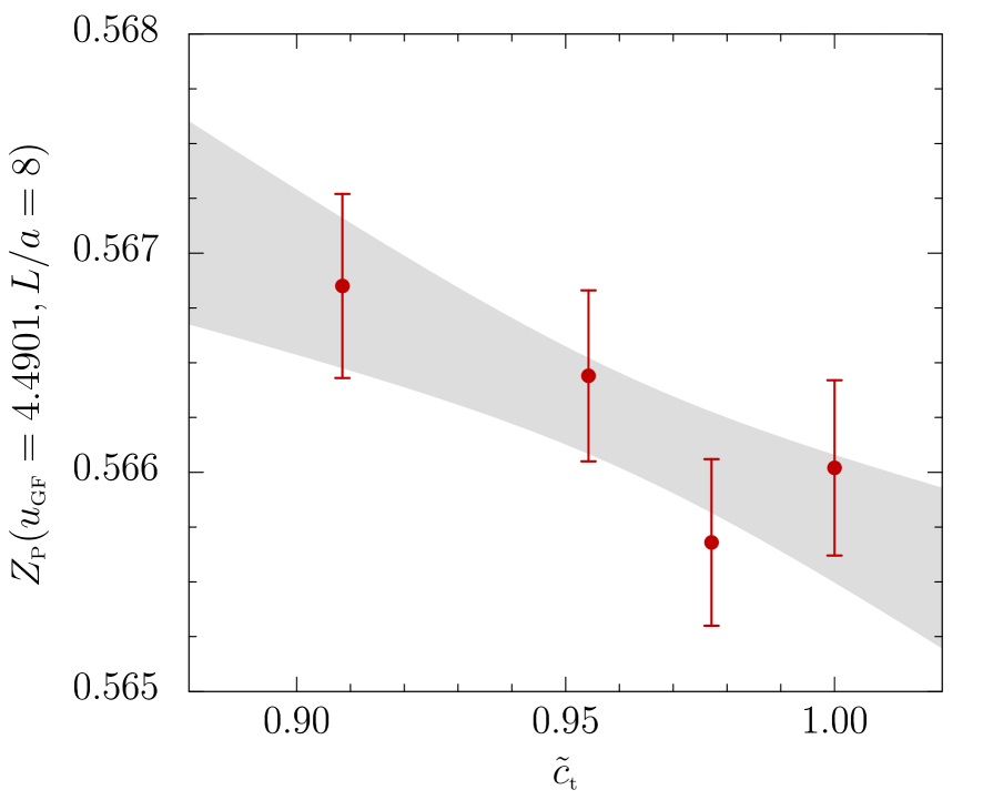
Figure 7: Variation of $Z_{\rm\scriptscriptstyle P}$ with the value of the boundary improvement coefficients $c_{\rm t}$ and $\tilde{c}_{\rm t}$. The shadowed bands are linear fits to the data.

We have performed dedicated simulations to estimate $(\partial Z_{\rm\scriptscriptstyle P}/\partial c_{\rm t})$ and $(\partial Z_{\rm\scriptscriptstyle P}/\partial\tilde{c}_{\rm t})$ in the ${\rm SF}$ scheme at $u=2.0120$ and in the ${\rm GF}$ scheme at $u=4.4901$, considering several values of $c_{\rm t}$ and $\tilde{c}_{\rm t}$ in an interval given by artificially augmenting the size of the perturbative correction to the tree-level value $1$ by factors of up to $4$. The simulations are performed in $L/a=6$ and $L/a=8$ lattices, which should be affected by the largest uncertainty. The results are illustrated in Fig. 7. By fitting the results for $Z_{\rm\scriptscriptstyle P}$ linearly in the value of the improvement coefficient we find

$$\left.\frac{\partial Z_{\rm\scriptscriptstyle P}}{\partial c_{\rm t}}\right|_{\scriptscriptstyle{\rm SF};L/a=6} =-0.016(15)\,,\qquad\qquad \left.\frac{\partial Z_{\rm\scriptscriptstyle P}}{\partial\tilde{c}_{\rm t}}\right|_{\scriptscriptstyle{\rm SF};L/a=6} =0.022(21)\,;$$ (A.74)

$$\left.\frac{\partial Z_{\rm\scriptscriptstyle P}}{\partial c_{\rm t}}\right|_{\scriptscriptstyle{\rm SF};L/a=8} =-0.003(26)\,,\qquad\qquad \left.\frac{\partial Z_{\rm\scriptscriptstyle P}}{\partial\tilde{c}_{\rm t}}\right|_{\scriptscriptstyle{\rm SF};L/a=8} =-0.074(19)\,;$$ (A.75)

$$\left.\frac{\partial Z_{\rm\scriptscriptstyle P}}{\partial c_{\rm t}}\right|_{\scriptscriptstyle{\rm GF};L/a=8} =0.110(14)\,,\qquad\qquad \left.\frac{\partial Z_{\rm\scriptscriptstyle P}}{\partial\tilde{c}_{\rm t}}\right|_{\scriptscriptstyle{\rm GF};L/a=8} =-0.090(4)\,.$$ (A.76)

If now we use values of $\Delta c_{\rm t}$ and $\Delta\tilde{c}_{\rm t}$ given by $1-c_{\rm t}^{\rm\scriptscriptstyle pert}$ and $1-\tilde{c}_{\rm t}^{\rm\scriptscriptstyle pert}$, respectively — i.e., we assign a $100\%$ uncertainty to the perturbative correction to the tree-level value $1$ — we finally obtain

$$u_{\rm\scriptscriptstyle SF} =2.0120\,,~{}L/a=6:\qquad \delta_{c_{\rm t}}\Sigma_{\rm\scriptscriptstyle P} \approx 0.00014\,,\quad \delta_{\tilde{c}_{\rm t}}\Sigma_{\rm\scriptscriptstyle P} \approx 0.000063\,;$$ (A.77)

$$u_{\rm\scriptscriptstyle SF} =2.0120\,,~{}L/a=8:\qquad \delta_{c_{\rm t}}\Sigma_{\rm\scriptscriptstyle P} \approx 0.000019\,,\quad \delta_{\tilde{c}_{\rm t}}\Sigma_{\rm\scriptscriptstyle P} \approx 0.00015\,;$$ (A.78)

$$u_{\rm\scriptscriptstyle GF} =4.4901\,,~{}L/a=8:\qquad \delta_{c_{\rm t}}\Sigma_{\rm\scriptscriptstyle P} \approx 0.00037\,,\quad \delta_{\tilde{c}_{\rm t}}\Sigma_{\rm\scriptscriptstyle P} \approx 0.00014\,.$$ (A.79)

In all cases, these figures are much smaller than the quoted statistical error of $\Sigma_{\rm\scriptscriptstyle P}$. This justifies neglecting this source of systematic uncertainty in our analysis.

B Simulation details

Our data is partly based on ensembles that have been produced in conjunction with the running coupling project [29, 31]. The low-energy ensembles are common to both projects, such that we had to take into account correlations between $Z_{\rm\scriptscriptstyle P}$ and $u_{\rm\scriptscriptstyle GF}$ as explained in section 4. To reach the desired precision in the computation of the mass anomalous dimension, the statistics on some of those ensembles had to be increased. Hence, we give a comprehensive list of the corresponding simulations in Table 10 which enter our data analysis.

The high-energy part is different in the respect that the computation of the SF coupling $u_{\rm\scriptscriptstyle SF}$, defining the lines of constant physics, is done with non-vanishing background gauge field, while $Z_{\rm\scriptscriptstyle P}$ is better computed with zero background field. As a result we have produced an independent set of ensembles summarised in Table 9. The bare parameters are inherited from the line of constant physics condition [29, 66].

Tables 9, 10 list the line of constant physics $(L/a,\beta,\kappa)$ for several fixed values of the renormalized coupling $u=\kern 1.0pt\overline{\kern-1.0ptg\kern 0.0pt}\kern 1.0pt^{2}(L)$, corresponding to a fixed scale $L$ in the continuum. The data are complemented by the number of measurements $N_{\rm ms}$ and their separation $\tau_{\rm ms}$ in molecular-dynamics (MD) units, the measured integrated autocorrelation times for $Z_{\rm\scriptscriptstyle P}$, values of the dimensionless bare current quark mass $Lm_{1}$, and the boundary-to-boundary correlator $f_{1}$.

C Tables

$u_{\rm\scriptscriptstyle SF}$	$L/a$	$\beta$	$\kappa$	$Z_{\rm\scriptscriptstyle P}(g_{0}^{2},L/a)$	$Z_{\rm\scriptscriptstyle P}(g_{0}^{2},2L/a)$	$\Sigma_{\rm\scriptscriptstyle P}^{\rm\scriptscriptstyle I}(g_{0}^{2},L/a)$	$\sigma_{\rm\scriptscriptstyle P}(u_{\rm\scriptscriptstyle SF})$	$\rho_{\rm\scriptscriptstyle P}(u_{\rm\scriptscriptstyle SF})$	$\chi^{2}/{\rm dof}$
	$6$	$8.5403$	$0.13233610$	$0.80494(22)$	$0.76879(24)$	$0.95587(40)(78)$
$1.11000$	$8$	$8.7325$	$0.13213380$	$0.79640(22)$	$0.76163(34)$	$0.95625(50)(10)$	$0.9577(10)$	$-0.079(56)$	$0.64$
	$12$	$8.9950$	$0.13186210$	$0.78473(29)$	$0.75167(59)$	$0.95762(83)(24)$
	$6$	$8.2170$	$0.13269030$	$0.79463(25)$	$0.75594(25)$	$0.95213(43)(82)$
$1.18446$	$8$	$8.4044$	$0.13247670$	$0.78532(21)$	$0.74943(39)$	$0.95420(56)(10)$	$0.9558(10)$	$-0.122(58)$	$0.50$
	$12$	$8.6769$	$0.13217153$	$0.77426(30)$	$0.73937(49)$	$0.95468(73)(25)$
	$6$	$7.9091$	$0.13305720$	$0.78344(24)$	$0.74256(25)$	$0.94870(44)(88)$
$1.26569$	$8$	$8.0929$	$0.13283120$	$0.77369(23)$	$0.73483(43)$	$0.94967(62)(11)$	$0.9512(10)$	$-0.093(61)$	$0.03$
	$12$	$8.3730$	$0.13249231$	$0.76349(33)$	$0.72601(49)$	$0.95064(76)(27)$
	$6$	$7.5909$	$0.13346930$	$0.77034(25)$	$0.72691(26)$	$0.94457(46)(94)$
$1.3627$	$8$	$7.7723$	$0.13322830$	$0.76036(24)$	$0.71893(42)$	$0.94539(63)(11)$	$0.9482(11)$	$-0.149(66)$	$1.11$
	$12$	$8.0578$	$0.13285365$	$0.74937(35)$	$0.71036(52)$	$0.94766(83)(29)$
	$6$	$7.2618$	$0.13393370$	$0.75460(27)$	$0.70808(31)$	$0.9394(5)(10)$
$1.4808$	$8$	$7.4424$	$0.13367450$	$0.74425(26)$	$0.70004(33)$	$0.94047(55)(13)$	$0.9415(11)$	$-0.071(66)$	$0.06$
	$12$	$7.7299$	$0.13326353$	$0.73515(33)$	$0.69193(42)$	$0.94090(72)(31)$
	$6$	$6.9433$	$0.13442200$	$0.73740(28)$	$0.68692(29)$	$0.9327(5)(11)$
$1.6173$	$8$	$7.1254$	$0.13414180$	$0.72670(26)$	$0.67983(49)$	$0.93536(76)(14)$	$0.9359(15)$	$-0.086(82)$	$2.56$
	$12$	$7.4107$	$0.13369922$	$0.71777(41)$	$0.67071(75)$	$0.9341(12)(3)$
	$6$	$6.6050$	$0.13498290$	$0.71606(29)$	$0.65960(32)$	$0.9224(6)(12)$
$1.7943$	$8$	$6.7915$	$0.13467650$	$0.70597(29)$	$0.65418(67)$	$0.9265(10)(2)$	$0.9298(15)$	$-0.250(84)$	$0.63$
	$12$	$7.0688$	$0.13420891$	$0.69553(40)$	$0.64543(63)$	$0.9276(11)(4)$
2.0120	$6$	$6.2735$	$0.13557130$	$0.69013(32)$	$0.62979(37)$	$0.9139(7)(13)$	0.9149(10)	$-0.006(69)$	0.59
	$8$	$6.4680$	$0.13523620$	$0.68107(28)$	$0.62341(43)$	$0.91518(74)(17)$
	$12$	$6.72995$	$0.13475973$	$0.67113(43)$	$0.61452(49)$	$0.91523(93)(41)$
	$16$	$6.93460$	$0.13441209$	$0.66627(31)$	$0.60924(66)$	$0.9141(11)(3)$

Table 6: Results for $Z_{\rm\scriptscriptstyle P}$, $\Sigma_{\rm\scriptscriptstyle P}^{\rm\scriptscriptstyle I}$, and $\sigma_{\rm\scriptscriptstyle P}$ in the ${\rm SF}$ scheme. The last three columns quote the value of $\sigma_{\rm\scriptscriptstyle P}$ obtained from a continuum-limit extrapolation fitting all three points linearly in $(a/L)^{2}$, the corresponding slope parameters, and the values of $\chi^{2}$ per degree of freedom (note that the numbers of degrees of freedom is always 1, save for the case $u=2.0120$ where it is 2).

Fit	$\left(\frac{L}{a}\right)_{\rm\scriptscriptstyle min}$	type	$n_{s}$	$n_{\rho}$	$\chi^{2}/\text{dof}$	$k=0$	$k=1$	$k=2$	$k=3$	$k=4$	$k=5$
$u_{k}$			–	–	–	2.0120	1.7126(31)	1.4939(38)	1.3264(38)	1.1936(35)	1.0856(32)
$\sigma_{\rm\scriptscriptstyle P}$:u-by-u	6	FITA	$4$	–	4.7/5	0.91522(98)	0.8528(13)	0.8034(16)	0.7626(17)	0.7280(17)	0.6980(18)
		FITA	$5$	–	4.4/4	0.91500(99)	0.8533(13)	0.8036(15)	0.7624(17)	0.7278(18)	0.6985(19)
		FITB	$4$	–	5.1/6	0.91540(99)	0.8526(13)	0.8030(14)	0.7622(16)	0.7278(17)	0.6982(19)
		FITB	$5$	–	3.3/5	0.91515(97)	0.8529(12)	0.8036(15)	0.7627(16)	0.7280(17)	0.6981(18)
$\sigma_{\rm\scriptscriptstyle P}$:global	6	FITA	$4$	$2$	19.1/21	0.91682(63)	0.85406(93)	0.8040(12)	0.7625(14)	0.7274(15)	0.6972(16)
		FITA	$5$	$3$	13.7/19	0.91550(85)	0.8528(12)	0.8031(14)	0.7623(15)	0.7278(17)	0.6982(19)
		FITB	$4$	$2$	20.2/22	0.91698(72)	0.8540(11)	0.8037(13)	0.7623(15)	0.7273(16)	0.6972(17)
		FITB	$5$	$3$	13.8/20	0.91551(94)	0.8527(13)	0.8031(15)	0.7623(17)	0.7278(18)	0.6981(19)
	8	FITA	$4$	$2$	12.9/13	0.9157(10)	0.8525(16)	0.8021(20)	0.7604(23)	0.7252(24)	0.6948(23)
		FITA	$5$	$3$	7.7/11	0.9142(11)	0.8514(15)	0.8017(17)	0.7608(20)	0.7264(22)	0.6970(25)
		FITB	$4$	$2$	14.3/14	0.91595(91)	0.8524(15)	0.8018(18)	0.7602(21)	0.7251(23)	0.6950(24)
		FITB	$5$	$3$	8.4/12	0.9143(12)	0.8513(16)	0.8016(19)	0.7608(21)	0.7264(24)	0.6967(26)
$\tau$:u-by-u	6	FITB	$2$	–	6.2/7	0.91794(86)	0.8552(13)	0.8051(15)	0.7636(16)	0.7286(17)	0.6984(17)
		FITB	$3$	–	3.5/6	0.9159(11)	0.8533(14)	0.8036(16)	0.7628(17)	0.7282(18)	0.6985(19)
		FITB	$4$	–	3.3/5	0.9156(11)	0.8532(13)	0.8037(16)	0.7629(17)	0.7282(17)	0.6983(18)
		FITB	$5$	–	2.4/4	0.9151(10)	0.8534(13)	0.8036(15)	0.7624(16)	0.7279(16)	0.6984(17)
$\tau$:global	6	FITA	$2$	$2$	18.5/22	0.91764(88)	0.8547(13)	0.8045(15)	0.7630(16)	0.7279(17)	0.6977(18)
		FITB	$2$	$2$	18.5/23	0.91763(98)	0.8547(14)	0.8044(16)	0.7630(17)	0.7279(18)	0.6971(18)
		FITB	$3$	$2$	18.4/22	0.91751(86)	0.8546(12)	0.8044(15)	0.7629(16)	0.7278(17)	0.6977(18)
		FITB	$2$	$3$	16.1/22	0.91775(96)	0.8550(13)	0.8048(15)	0.7631(17)	0.7283(17)	0.6981(18)
		FITB	$3$	$3$	13.0/21	0.9155(12)	0.8527(14)	0.8031(15)	0.7623(16)	0.7278(17)	0.6981(18)
	8	FITA	$2$	$2$	12.0/14	0.9166(11)	0.8532(16)	0.8026(19)	0.7608(21)	0.7256(22)	0.6954(24)
		FITB*	$2$	$2$	12.0/15	0.9165(12)	0.8530(17)	0.8025(20)	0.7608(21)	0.7257(22)	0.6955(23)
		FITB	$3$	$2$	12.0/14	0.9166(10)	0.8531(15)	0.8025(18)	0.7608(21)	0.7257(22)	0.6954(23)
		FITB	$2$	$3$	10.0/14	0.9165(12)	0.8532(16)	0.8027(19)	0.7611(21)	0.7260(21)	0.6958(22)
		FITB	$3$	$3$	7.3/13	0.9144(14)	0.8514(17)	0.8017(19)	0.7609(21)	0.7264(23)	0.6968(24)
PT prediction	–	s1,s2	–	–	13/8	0.90797	0.84057	0.78808	0.74552	0.70998	0.67966

Table 7: Mass-ratios $R^{(k)}$, cf. Eqs. (3.45) and (3.48), as obtained from different analysis procedures. The quoted values of $u_{k}$ have been obtained using Eq. (2.34) with $b^{\rm eff}_{3}$.

$u_{\rm\scriptscriptstyle GF}$	$L/a$	$\beta$	$\kappa$	$Z_{\rm\scriptscriptstyle P}(g_{0}^{2},L/a)$	$Z_{\rm\scriptscriptstyle P}(g_{0}^{2},2L/a)$	$\Sigma_{\rm\scriptscriptstyle P}(g_{0}^{2},L/a)$
$2.1269(15)$	$8$	$5.371500$	$0.13362120$	$0.73275(26)$	$0.67666(55)$	$0.92345(82)$
$2.1229(12)$	$12$	$5.543070$	$0.13331407$	$0.71301(33)$	$0.65748(85)$	$0.9221(12)$
$2.1257(25)$	$16$	$5.700000$	$0.13304840$	$0.70248(31)$	$0.64369(85)$	$0.9163(13)$
$2.3913(15)$	$8$	$5.071000$	$0.13421678$	$0.71024(32)$	$0.64872(59)$	$0.91338(93)$
$2.3912(10)$	$12$	$5.242465$	$0.13387635$	$0.69064(30)$	$0.62808(99)$	$0.9094(15)$
$2.3900(32)$	$16$	$5.400000$	$0.13357851$	$0.67890(35)$	$0.61636(95)$	$0.9079(15)$
$2.7365(14)$	$8$	$4.764900$	$0.13488555$	$0.68196(32)$	$0.61339(69)$	$0.8995(11)$
$2.7390(14)$	$12$	$4.938726$	$0.13450761$	$0.66137(42)$	$0.59091(84)$	$0.8935(14)$
$2.7359(36)$	$16$	$5.100000$	$0.13416889$	$0.65087(41)$	$0.58199(92)$	$0.8942(15)$
$3.2022(16)$	$8$	$4.457600$	$0.13560675$	$0.64779(34)$	$0.56891(78)$	$0.8782(13)$
$3.2053(17)$	$12$	$4.634654$	$0.13519986$	$0.62622(39)$	$0.54748(98)$	$0.8743(16)$
$3.2029(49)$	$16$	$4.800000$	$0.13482139$	$0.61735(43)$	$0.5382(11)$	$0.8717(19)$
$3.8620(20)$	$8$	$4.151900$	$0.13632589$	$0.60377(37)$	$0.51002(78)$	$0.8447(14)$
$3.8635(21)$	$12$	$4.331660$	$0.13592664$	$0.58285(49)$	$0.4887(14)$	$0.8384(26)$
$3.8643(64)$	$16$	$4.500000$	$0.13552582$	$0.57420(48)$	$0.4822(14)$	$0.8398(25)$
$4.4855(25)$	$8$	$3.947900$	$0.13674684$	$0.56568(39)$	$0.4570(11)$	$0.8079(21)$
$4.4867(28)$	$12$	$4.128217$	$0.13640300$	$0.54608(62)$	$0.4331(10)$	$0.7931(21)$
$4.4901(75)$	$16$	$4.300000$	$0.13600821$	$0.54030(55)$	$0.4266(16)$	$0.7895(30)$
$5.2928(28)$	$8$	$3.754890$	$0.13701929$	$0.52174(43)$	$0.3928(29)$	$0.7528(57)$
$5.2972(36)$	$12$	$3.936816$	$0.13679805$	$0.50367(57)$	$0.3642(21)$	$0.7231(41)$
$5.301(14)$	$16$	$4.100000$	$0.13647301$	$0.49847(79)$	$0.3579(28)$	$0.7179(54)$

Table 8: Results for $Z_{\rm\scriptscriptstyle P}$ and $\Sigma_{\rm\scriptscriptstyle P}$ in the ${\rm GF}$ scheme.

$u_{\rm\scriptscriptstyle SF}$	$L/a$	$\beta$	$\kappa$	$s$	$N_{\rm ms}$	$\dfrac{\tau_{\rm ms}}{\tau}$	$\dfrac{\tau_{\rm int}[Z_{\rm\scriptscriptstyle P}]}{\tau_{\rm ms}}$	$10^{2}Lm_{1}$	$f_{1}$
$1.11000$	$6$	$8.5403$	$0.13233610$	$1$	$5000$	$5$	$0.50(2)$	$-0.74(4)$	$0.9706(11)$
				$2$	$5000$	$5$	$0.76(7)$	$-1.60(3)$	$0.8929(12)$
	$8$	$8.7325$	$0.13213380$	$1$	$5000$	$5$	$0.58(5)$	$-0.97(3)$	$0.9526(10)$
				$2$	$2683$	$5$	$0.92(13)$	$-1.81(3)$	$0.8795(21)$
	$12$	$8.9950$	$0.13186210$	$1$	$2769$	$5$	$0.72(9)$	$-0.64(3)$	$0.9161(16)$
				$2$	$1576$	$5$	$1.71(39)$	$-1.14(3)$	$0.8412(40)$
$1.18446$	$6$	$8.2170$	$0.13269030$	$1$	$5000$	$5$	$0.56(4)$	$-0.74(4)$	$0.9428(11)$
				$2$	$5000$	$5$	$0.75(7)$	$-1.63(3)$	$0.8690(12)$
	$8$	$8.4044$	$0.13247670$	$1$	$5000$	$5$	$0.49(1)$	$-1.00(3)$	$0.9276(10)$
				$2$	$2314$	$5$	$0.89(13)$	$-1.91(4)$	$0.8525(29)$
	$12$	$8.6769$	$0.13217153$	$1$	$2476$	$5$	$0.60(7)$	$-0.76(4)$	$0.8938(17)$
				$2$	$3759$	$5$	$2.45(46)$	$-1.25(2)$	$0.8176(23)$
$1.26569$	$6$	$7.9091$	$0.13305720$	$1$	$5000$	$5$	$0.50(1)$	$-0.74(4)$	$0.9160(11)$
				$2$	$5000$	$5$	$0.72(7)$	$-1.73(3)$	$0.8393(13)$
	$8$	$8.0929$	$0.13283120$	$1$	$5000$	$5$	$0.54(4)$	$-1.08(4)$	$0.9005(11)$
				$2$	$2273$	$5$	$1.01(16)$	$-1.98(4)$	$0.8252(21)$
	$12$	$8.3730$	$0.13249231$	$1$	$2729$	$5$	$0.71(9)$	$-0.76(4)$	$0.8654(18)$
				$2$	$3749$	$5$	$2.20(40)$	$-1.35(2)$	$0.7926(32)$
$1.3627$	$6$	$7.5909$	$0.13346930$	$1$	$5000$	$5$	$0.50(2)$	$-0.81(5)$	$0.8877(11)$
				$2$	$5000$	$5$	$0.69(6)$	$-1.63(3)$	$0.8034(15)$
	$8$	$7.7723$	$0.13322830$	$1$	$5000$	$5$	$0.57(5)$	$-1.18(4)$	$0.8725(11)$
				$2$	$2163$	$5$	$0.86(13)$	$-2.12(5)$	$0.7892(36)$
	$12$	$8.0578$	$0.13285365$	$1$	$2448$	$5$	$0.71(9)$	$-0.81(4)$	$0.8423(17)$
				$2$	$3762$	$5$	$2.42(45)$	$-1.49(2)$	$0.7594(29)$

Table 9: Details for SF simulations of $(s\times L/a)^{4}$ lattices with vanishing background field and plaquette gauge action, cf. Section 3. Each trajectory has a length of $\tau=2$ MD units, and lines of constant physics (fixed $u_{\rm\scriptscriptstyle SF}$) are set with background field as reported in Refs. [29, 96] (continues on the next page).

$u_{\rm\scriptscriptstyle SF}$	$L/a$	$\beta$	$\kappa$	$s$	$N_{\rm ms}$	$\dfrac{\tau_{\rm ms}}{\tau}$	$\dfrac{\tau_{\rm int}[Z_{\rm\scriptscriptstyle P}]}{\tau_{\rm ms}}$	$10^{2}Lm_{1}$	$f_{1}$
$1.4808$	$6$	$7.2618$	$0.13393370$	$1$	$5000$	$5$	$0.49(1)$	$-0.87(5)$	$0.8547(11)$
				$2$	$5000$	$5$	$0.87(9)$	$-1.50(4)$	$0.7658(16)$
	$8$	$7.4424$	$0.13367450$	$1$	$5000$	$5$	$0.60(5)$	$-1.15(4)$	$0.8385(11)$
				$2$	$4500$	$5$	$0.99(12)$	$-2.09(3)$	$0.7529(17)$
	$12$	$7.7299$	$0.13326353$	$1$	$2710$	$5$	$0.67(8)$	$-0.88(4)$	$0.8119(20)$
				$2$	$6343$	$5$	$2.33(34)$	$-1.49(3)$	$0.7226(23)$
$1.6173$	$6$	$6.9433$	$0.13442200$	$1$	$5000$	$5$	$0.50(3)$	$-0.76(5)$	$0.8152(13)$
				$2$	$5000$	$5$	$0.68(6)$	$-1.39(4)$	$0.7219(15)$
	$8$	$7.1254$	$0.13414180$	$1$	$5000$	$5$	$0.56(4)$	$-1.12(5)$	$0.8058(12)$
				$2$	$2041$	$5$	$0.87(14)$	$-2.06(5)$	$0.7172(29)$
	$12$	$7.4107$	$0.13369922$	$1$	$2535$	$5$	$0.80(11)$	$-0.87(5)$	$0.7740(20)$
				$2$	$3412$	$5$	$3.88(91)$	$-1.59(3)$	$0.6851(31)$
$1.7943$	$6$	$6.6050$	$0.13498290$	$1$	$5000$	$5$	$0.49(1)$	$-0.80(6)$	$0.7743(13)$
				$2$	$5000$	$5$	$0.76(7)$	$-1.18(4)$	$0.6742(17)$
	$8$	$6.7915$	$0.13467650$	$1$	$5000$	$5$	$0.57(5)$	$-1.17(6)$	$0.7637(13)$
				$2$	$1807$	$5$	$1.35(26)$	$-2.10(6)$	$0.6688(40)$
	$12$	$7.0688$	$0.13420891$	$1$	$2339$	$5$	$0.68(8)$	$-0.83(6)$	$0.7311(22)$
				$2$	$2607$	$5$	$1.94(38)$	$-1.48(4)$	$0.6351(33)$
$2.0120$	$6$	$6.2735$	$0.13557130$	$1$	$5000$	$5$	$0.53(4)$	$-0.69(7)$	$0.7233(13)$
				$2$	$4435$	$5$	$0.85(9)$	$-0.92(5)$	$0.6209(21)$
	$8$	$6.4680$	$0.13523620$	$1$	$5000$	$5$	$0.53(4)$	$-1.14(6)$	$0.7204(14)$
				$2$	$4048$	$5$	$1.04(13)$	$-1.93(5)$	$0.6155(20)$
	$10$	$6.60959$	$0.13497763$	$1$	$6240$	$5$	$0.72(6)$	$-1.08(4)$	$0.7018(14)$
	$12$	$6.72995$	$0.13475973$	$1$	$3000$	$5$	$0.86(11)$	$-0.80(6)$	$0.6915(19)$
				$2$	$5094$	$5$	$2.42(40)$	$-1.44(3)$	$0.5808(55)$
				$2$	$512$	$10$	$1.14(34)$	$-1.33(10)$	$0.5833(25)$
	$16$	$6.93460$	$0.13441209$	$1$	$4604$	$10$	$0.73(7)$	$-0.51(4)$	$0.6655(16)$
				$2$	$2325$	$10$	$1.69(3)$	$-1.01(4)$	$0.5583(44)$

Table 9: (continued)

$u_{\rm\scriptscriptstyle GF}$	$L/a$	$\beta$	$\kappa$	$s$	$N_{\rm ms}$	$\dfrac{\tau_{\rm ms}}{\text{MD}}$	$\dfrac{\tau_{\rm int}[Z_{\rm\scriptscriptstyle P}]}{\tau_{\rm ms}}$	$10^{2}Lm_{1}$	$f_{1}$
$2.1257$	$8$	$5.371500$	$0.13362120$	$1$	$5001$	$10$	$0.53(4)$	$+0.03(5)$	$0.8471(14)$
				$2$	$2001$	$10$	$1.21(22)$	$+0.52(5)$	$0.7175(40)$
	$12$	$5.543070$	$0.13331407$	$1$	$8000$	$5$	$1.35(14)$	$+0.13(3)$	$0.7962(15)$
				$2$	$2400$	$10$	$3.17(58)$	$+0.62(4)$	$0.6618(53)$
	$16$	$5.700000$	$0.13304840$	$1$	$7001$	$10$	$1.26(14)$	$-0.04(3)$	$0.7697(19)$
				$2$	$500$	$100$	$0.54(11)$	$+0.38(7)$	$0.6414(51)$
$2.3900$	$8$	$5.071000$	$0.13421678$	$1$	$5001$	$10$	$0.58(5)$	$+0.02(5)$	$0.8092(15)$
				$2$	$2001$	$10$	$1.09(19)$	$+0.66(6)$	$0.6677(37)$
	$12$	$5.242465$	$0.13387635$	$1$	$8000$	$5$	$1.22(12)$	$+0.05(4)$	$0.7602(18)$
				$2$	$2400$	$10$	$3.21(59)$	$+0.64(4)$	$0.6145(53)$
	$16$	$5.400000$	$0.13357851$	$1$	$6001$	$10$	$1.16(13)$	$+0.07(3)$	$0.7263(23)$
				$2$	$500$	$100$	$0.68(13)$	$+0.59(9)$	$0.5970(42)$
$2.7359$	$8$	$4.764900$	$0.13488555$	$1$	$5001$	$10$	$0.59(5)$	$+0.04(6)$	$0.7675(14)$
				$2$	$2001$	$10$	$1.36(26)$	$+0.91(7)$	$0.6185(36)$
	$12$	$4.938726$	$0.13450761$	$1$	$5001$	$5$	$1.13(13)$	$+0.06(6)$	$0.7123(25)$
				$2$	$2400$	$10$	$2.45(41)$	$+0.78(5)$	$0.5607(57)$
	$16$	$5.100000$	$0.13416889$	$1$	$6001$	$10$	$1.23(14)$	$+0.04(3)$	$0.6814(21)$
				$2$	$500$	$100$	$0.74(14)$	$+0.67(8)$	$0.5385(42)$
$3.2029$	$8$	$4.457600$	$0.13560675$	$1$	$5001$	$10$	$0.55(4)$	$+0.09(7)$	$0.7239(16)$
				$2$	$2001$	$10$	$1.20(22)$	$+1.10(9)$	$0.5524(65)$
	$12$	$4.634654$	$0.13519986$	$1$	$5001$	$5$	$1.05(12)$	$+0.06(6)$	$0.6684(30)$
				$2$	$2400$	$10$	$2.88(51)$	$+0.68(6)$	$0.5052(57)$
	$16$	$4.800000$	$0.13482139$	$1$	$5000$	$10$	$1.31(17)$	$+0.12(4)$	$0.6307(25)$
				$2$	$2000$	$20$	$2.47(44)$	$+0.79(5)$	$0.4813(51)$
$3.8643$	$8$	$4.151900$	$0.13632589$	$1$	$5001$	$10$	$0.58(5)$	$-0.07(9)$	$0.6798(19)$
				$2$	$2001$	$10$	$1.23(23)$	$+1.58(10)$	$0.4866(51)$
	$12$	$4.331660$	$0.13592664$	$1$	$5001$	$5$	$1.19(15)$	$-0.10(8)$	$0.6190(29)$
				$2$	$2400$	$10$	$3.17(58)$	$+0.77(7)$	$0.4381(78)$
	$16$	$4.500000$	$0.13552582$	$1$	$5000$	$10$	$1.30(17)$	$+0.00(5)$	$0.5805(24)$
				$2$	$2000$	$20$	$3.07(60)$	$+0.68(6)$	$0.3921(80)$

Table 10: Details for SF simulations of $(s\times L/a)^{4}$ lattices with vanishing background field and tree-level Symanzik improved gauge action, cf. Section 4. Lines of constant physics (fixed $u_{\rm\scriptscriptstyle GF}$) are set as reported in Ref. [31] (continues on the next page).

$u_{\rm\scriptscriptstyle GF}$	$L/a$	$\beta$	$\kappa$	$s$	$N_{\rm ms}$	$\dfrac{\tau_{\rm ms}}{\text{MD}}$	$\dfrac{\tau_{\rm int}[Z_{\rm\scriptscriptstyle P}]}{\tau_{\rm ms}}$	$10^{2}Lm_{1}$	$f_{1}$
$4.4901$	$8$	$3.947900$	$0.13674684$	$1$	$5001$	$10$	$0.61(6)$	$-0.11(10)$	$0.6385(19)$
				$2$	$2001$	$10$	$2.04(46)$	$+2.02(11)$	$0.4297(56)$
	$12$	$4.128217$	$0.13640300$	$1$	$5001$	$5$	$1.84(27)$	$-0.07(9)$	$0.5802(33)$
				$2$	$4127$	$10$	$3.81(60)$	$+1.03(7)$	$0.3622(55)$
	$16$	$4.300000$	$0.13600821$	$1$	$5000$	$10$	$1.56(22)$	$-0.00(6)$	$0.5343(27)$
				$2$	$3439$	$20$	$5.1(1.0)$	$+0.86(5)$	$0.3338(57)$
$5.3010$	$8$	$3.754890$	$0.13701929$	$1$	$5001$	$5$	$0.84(9)$	$+0.23(14)$	$0.6094(30)$
				$2$	$2001$	$10$	$8.6(3.4)$	$+3.17(16)$	$0.3474(95)$
	$12$	$3.936816$	$0.13679805$	$1$	$5001$	$5$	$1.13(14)$	$-0.18(10)$	$0.5326(33)$
				$2$	$3682$	$10$	$7.6(2.2)$	$+1.54(8)$	$0.2878(78)$
	$16$	$4.100000$	$0.13647301$	$1$	$3200$	$10$	$1.48(24)$	$-0.04(8)$	$0.4898(43)$
				$2$	$2674$	$20$	$11.8(4.7)$	$+1.04(7)$	$0.2612(72)$
$5.8673$	$8$	$3.653850$	$0.13707221$	$1$	$5001$	$5$	$8.97(10)$	$+0.10(16)$	$0.5941(31)$
				$2$	$2000$	$10$	$3.7(1.0)$	$+4.82(22)$	$0.3168(72)$
	$12$	$3.833254$	$0.13696774$	$1$	$5001$	$5$	$2.00(31)$	$+0.14(11)$	$0.5139(37)$
				$2$	$2400$	$10$	$11.8(4.8)$	$+2.03(13)$	$0.2360(79)$
	$16$	$4.000000$	$0.13668396$	$1$	$4602$	$10$	$1.45(20)$	$+0.06(8)$	$0.4663(35)$
				$2$	$1404$	$20$	$32(20)$	$+1.71(12)$	$0.1895(16)$
$6.5489$	$8$	$3.556470$	$0.13703245$	$1$	$5001$	$5$	$1.03(11)$	$-0.18(19)$	$0.5871(36)$
				$2$	$2000$	$10$	$4.7(1.5)$	$+7.69(34)$	$0.2304(72)$
	$12$	$3.735394$	$0.13708263$	$1$	$5001$	$5$	$1.53(21)$	$-0.06(14)$	$0.4905(43)$
				$2$	$3000$	$10$	$19.2(8.7)$	$+2.74(16)$	$0.1864(69)$
	$16$	$3.900000$	$0.13687202$	$1$	$4600$	$10$	$1.60(23)$	$+0.08(8)$	$0.4360(35)$
				$2$	$1205$	$20$	$11.4(5.9)$	$+1.87(21)$	$0.1656(91)$

Table 10: (continued)

References

• [1] A. Denner, S. Heinemeyer, I. Puljak, D. Rebuzzi and M. Spira, Eur. Phys. J. C 71 (2011) 1753 [arXiv:1107.5909 [hep-ph]].
• [2] S. Heinemeyer et al. [LHC Higgs Cross Section Working Group], arXiv:1307.1347 [hep-ph].
• [3] L. G. Almeida, S. J. Lee, S. Pokorski and J. D. Wells, Phys. Rev. D 89 (2014) no.3, 033006 [arXiv:1311.6721 [hep-ph]].
• [4] G. P. Lepage, P. B. Mackenzie and M. E. Peskin, arXiv:1404.0319 [hep-ph].
• [5] A. A. Petrov, S. Pokorski, J. D. Wells and Z. Zhang, Phys. Rev. D 91 (2015) no.7, 073001 [arXiv:1501.02803 [hep-ph]].
• [6] S. Aoki et al., Eur. Phys. J. C 74 (2014) 2890 [arXiv:1310.8555 [hep-lat]].
• [7] S. Aoki et al., Eur. Phys. J. C 77 (2017) no.2, 112 [arXiv:1607.00299 [hep-lat]].
• [8] A. Bazavov et al. [MILC Collaboration], PoS CD 09 (2009) 007 [arXiv:0910.2966 [hep-ph]].
• [9] C. McNeile, C. T. H. Davies, E. Follana, K. Hornbostel and G. P. Lepage [HPQCD Collaboration], Phys. Rev. D 82 (2010) 034512 [arXiv:1004.4285 [hep-lat]].
• [10] A. Bazavov et al., PoS LATTICE 2010 (2010) 083 [arXiv:1011.1792 [hep-lat]].
• [11] S. Dürr et al. [BMW Collaboration], Phys. Lett. B 701 (2011) 265 [arXiv:1011.2403 [hep-lat]].
• [12] S. Dürr et al. [BMW Collaboration], JHEP 1108 (2011) 148 [arXiv:1011.2711 [hep-lat]].
• [13] B. Blossier et al. [ETM Collaboration], Phys. Rev. D 82 (2010) 114513 [arXiv:1010.3659 [hep-lat]].
• [14] P. Fritzsch et al. [ALPHA Collaboration], Nucl. Phys. B 865 (2012) 397 [arXiv:1205.5380 [hep-lat]].
• [15] N. Carrasco et al. [ETM Collaboration], JHEP 1403 (2014) 016 [arXiv:1308.1851 [hep-lat]].
• [16] F. Bernardoni et al. [ALPHA Collaboration], Phys. Lett. B 730 (2014) 171 [arXiv:1311.5498 [hep-lat]].
• [17] N. Carrasco et al. [ETM Collaboration], Nucl. Phys. B 887 (2014) 19 [arXiv:1403.4504 [hep-lat]].
• [18] C. Alexandrou, V. Drach, K. Jansen, C. Kallidonis and G. Koutsou, Phys. Rev. D 90 (2014) no.7, 074501 [arXiv:1406.4310 [hep-lat]].
• [19] B. Colquhoun, R. J. Dowdall, C. T. H. Davies, K. Hornbostel and G. P. Lepage [HPQCD Collaboration], Phys. Rev. D 91 (2015) no.7, 074514 [arXiv:1408.5768 [hep-lat]].
• [20] B. Chakraborty et al. [HPQCD Collaboration], Phys. Rev. D 91 (2015) no.5, 054508 [arXiv:1408.4169 [hep-lat]].
• [21] Y. B. Yang et al. [$\chi$QCD Collaboration], Phys. Rev. D 92 (2015) no.3, 034517 [arXiv:1410.3343 [hep-lat]].
• [22] T. Blum et al. [RBC and UKQCD Collaborations], Phys. Rev. D 93 (2016) no.7, 074505 [arXiv:1411.7017 [hep-lat]].
• [23] K. G. Chetyrkin, Phys. Lett. B 404 (1997) 161 [hep-ph/9703278].
• [24] J. A. M. Vermaseren, S. A. Larin and T. van Ritbergen, Phys. Lett. B 405 (1997) 327 [hep-ph/9703284].
• [25] J. A. Gracey, Nucl. Phys. B 662 (2003) 247 [hep-ph/0304113].
• [26] I. Campos et al. [ALPHA Collaboration], PoS LATTICE 2015 (2016) 249 [arXiv:1508.06939 [hep-lat]].
• [27] I. Campos et al. [ALPHA Collaboration], EPJ Web Conf.  137 (2017) 08006 [arXiv:1611.06102 [hep-lat]].
• [28] I. Campos et al. [ALPHA Collaboration], PoS LATTICE 2016 (2016) 201 [arXiv:1611.09711 [hep-lat]].
• [29] M. Dalla Brida et al. [ALPHA Collaboration], Phys. Rev. Lett.  117 (2016) no.18, 182001 [arXiv:1604.06193 [hep-ph]].
• [30] M. Dalla Brida et al. [ALPHA Collaboration], Eur. Phys. J. C 78 (2018) no.5, 372 [arXiv:1803.10230 [hep-lat]].
• [31] M. Dalla Brida et al. [ALPHA Collaboration], Phys. Rev. D 95 (2017) no.1, 014507 [arXiv:1607.06423 [hep-lat]].
• [32] M. Bruno et al. [ALPHA Collaboration], Phys. Rev. Lett.  119 (2017) no.10, 102001 [arXiv:1706.03821 [hep-lat]].
• [33] M. Lüscher, R. Narayanan, P. Weisz and U. Wolff, Nucl. Phys. B 384 (1992) 168 [hep-lat/9207009].
• [34] S. Sint, Nucl. Phys. B 421 (1994) 135 [hep-lat/9312079].
• [35] S. Capitani, M. Lüscher, R. Sommer and H. Wittig [ALPHA Collaboration], Nucl. Phys. B 544 (1999) 669 Erratum: [Nucl. Phys. B 582 (2000) 762] [hep-lat/9810063].
• [36] M. Della Morte et al. [ALPHA Collaboration], Nucl. Phys. B 729 (2005) 117 [hep-lat/0507035].
• [37] M. Guagnelli et al. [ALPHA Collaboration], JHEP 0603 (2006) 088 [hep-lat/0505002].
• [38] F. Palombi, C. Pena and S. Sint [ALPHA Collaboration], JHEP 0603 (2006) 089 [hep-lat/0505003].
• [39] P. Dimopoulos et al., Phys. Lett. B 641 (2006) 118 [hep-lat/0607028].
• [40] P. Dimopoulos et al. [ALPHA Collaboration], JHEP 0805 (2008) 065 [arXiv:0712.2429 [hep-lat]].
• [41] F. Palombi, M. Papinutto, C. Pena and H. Wittig [ALPHA Collaboration], JHEP 0709 (2007) 062 [arXiv:0706.4153 [hep-lat]].
• [42] B. Blossier, M. Della Morte, N. Garron and R. Sommer [ALPHA Collaboration], JHEP 1006 (2010) 002 [arXiv:1001.4783 [hep-lat]].
• [43] F. Bernardoni et al. [ALPHA Collaboration], Phys. Lett. B 735 (2014) 349 [arXiv:1404.3590 [hep-lat]].
• [44] M. Papinutto, C. Pena and D. Preti [ALPHA Collaboration], Eur. Phys. J. C 77 (2017) no.6, 376 Erratum: [Eur. Phys. J. C 78 (2018) no.1, 21] [arXiv:1612.06461 [hep-lat]].
• [45] P. Dimopoulos et al. [ALPHA Collaboration], arXiv:1801.09455 [hep-lat].
• [46] C. Pena and D. Preti [ALPHA Collaboration], arXiv:1706.06674 [hep-lat].
• [47] M. Bruno et al., JHEP 1502 (2015) 043 [arXiv:1411.3982 [hep-lat]].
• [48] S. Weinberg, Phys. Rev. D 8 (1973) 3497.
• [49] G. ’t Hooft, Nucl. Phys. B 61 (1973) 455.
• [50] V. S. Vanyashin and M. V. Terent’ev, JETP 21 (1965) 375.
• [51] I. B. Khriplovich, Sov. J. Nucl. Phys.  10 (1969) 235 [Yad. Fiz.  10 (1969) 409].
• [52] G. ’t Hooft , report at the Colloquium on Renormalization of Yang-Mills Fields and Applications to Particle Physics, Marseille, France, June 1972 (unpublished).
• [53] D. J. Gross and F. Wilczek, Phys. Rev. Lett.  30 (1973) 1343.
• [54] H. D. Politzer, Phys. Rev. Lett.  30 (1973) 1346.
• [55] W. E. Caswell, Phys. Rev. Lett.  33 (1974) 244.
• [56] D. R. T. Jones, Nucl. Phys. B 75 (1974) 531.
• [57] M. Lüscher, S. Sint, R. Sommer and P. Weisz, Nucl. Phys. B 478 (1996) 365 [hep-lat/9605038].
• [58] K. Symanzik, Nucl. Phys. B 190 (1981) 1.
• [59] M. Lüscher, Nucl. Phys. B 254 (1985) 52.
• [60] S. Sint, Nucl. Phys. B 451 (1995) 416 doi:10.1016/0550-3213(95)00352-S [hep-lat/9504005].
• [61] P. Fritzsch and A. Ramos, JHEP 1310 (2013) 008 [arXiv:1301.4388 [hep-lat]].
• [62] A. Ramos, PoS LATTICE 2014 (2015) 017 [arXiv:1506.00118 [hep-lat]].
• [63] A. Bode et al. [ALPHA Collaboration], Nucl. Phys. B 576 (2000) 517 Erratum: [Nucl. Phys. B 608 (2001) 481] Erratum: [Nucl. Phys. B 600 (2001) 453] [hep-lat/9911018].
• [64] S. Sint et al. [ALPHA Collaboration], Nucl. Phys. B 545 (1999) 529 [hep-lat/9808013].
• [65] U. Wolff [ALPHA Collaboration], Comput. Phys. Commun.  156 (2004) 143 Erratum: [Comput. Phys. Commun.  176 (2007) 383] [hep-lat/0306017].
• [66] P. Fritzsch and T. Korzec, in preparation.
• [67] K. G. Wilson, Phys. Rev. D 10 (1974) 2445.
• [68] B. Sheikholeslami and R. Wohlert, Nucl. Phys. B 259 (1985) 572.
• [69] N. Yamada et al. [JLQCD and CP-PACS Collaborations], Phys. Rev. D 71 (2005) 054505 [hep-lat/0406028].
• [70] M. Lüscher and P. Weisz, Nucl. Phys. B 479 (1996) 429 [hep-lat/9606016].
• [71] A. Bode et al. [ALPHA Collaboration], Nucl. Phys. B 540 (1999) 491 [hep-lat/9809175].
• [72] M. Lüscher and S. Schaefer, Comput. Phys. Commun.  184 (2013) 519 [arXiv:1206.2809 [hep-lat]].
• [73] M. Lüscher and S. Schaefer, “openQCD simulation program for lattice QCD with open boundary conditions,” http://luscher.web.cern.ch/luscher/openQCD/.
• [74] M. Lüscher and P. Weisz, Phys. Lett.  158B (1985) 250.
• [75] J. Bulava and S. Schaefer, Nucl. Phys. B 874 (2013) 188 [arXiv:1304.7093 [hep-lat]].
• [76] S. Takeda, S. Aoki and K. Ide, Phys. Rev. D 68 (2003) 014505 [hep-lat/0304013].
• [77] Pol Vilaseca, private communication.
• [78] S. Schaefer et al. [ALPHA Collaboration], Nucl. Phys. B 845 (2011) 93 [arXiv:1009.5228 [hep-lat]].
• [79] P. Fritzsch, A. Ramos and F. Stollenwerk, PoS Lattice 2013 (2014) 461 [arXiv:1311.7304 [hep-lat]].
• [80] J. Bulava et al. [ALPHA Collaboration], Nucl. Phys. B 896 (2015) 555 [arXiv:1502.04999 [hep-lat]].
• [81] J. Bulava, M. Della Morte, J. Heitger and C. Wittemeier [ALPHA Collaboration], Phys. Rev. D 93 (2016) no.11, 114513 [arXiv:1604.05827 [hep-lat]].
• [82] M. Dalla Brida, S. Sint and P. Vilaseca, JHEP 1608 (2016) 102 [arXiv:1603.00046 [hep-lat]].
• [83] M. Dalla Brida, T. Korzec, S. Sint and P. Vilaseca, in preparation
• [84] S. Sint, Nucl. Phys. B 847 (2011) 491 [arXiv:1008.4857 [hep-lat]].
• [85] S. Sint and B. Leder, PoS LATTICE 2010 (2010) 265 [arXiv:1012.2500 [hep-lat]].
• [86] M. Dalla Brida and S. Sint, PoS LATTICE 2014 (2014) 280 [arXiv:1412.8022 [hep-lat]].
• [87] D. Mohler, S. Schaefer and J. Simeth, arXiv:1712.04884 [hep-lat].
• [88] R. Frezzotti et al. [ALPHA Collaboration], JHEP 0108 (2001) 058 [hep-lat/0101001].
• [89] [ALPHA Collaboration], to appear.
• [90] M. Bruno, T. Korzec and S. Schaefer, Phys. Rev. D 95 (2017) no.7, 074504 [arXiv:1608.08900 [hep-lat]].
• [91] G. Herdoíza, C. Pena, D. Preti, J. Á. Romero and J. Ugarrio, arXiv:1711.06017 [hep-lat].
• [92] F. Knechtli et al. [ALPHA Collaboration], Phys. Lett. B 774 (2017) 649 [arXiv:1706.04982 [hep-lat]].
• [93] S. Calì, F. Knechtli, T. Korzec and H. Panagopoulos, arXiv:1710.06221 [hep-lat].
• [94] F. Knechtli, T. Korzec, B. Leder and G. Moir [ALPHA Collaboration], arXiv:1710.07590 [hep-lat].
• [95] R. Sommer, “The critical line for the $N_{\mathrm{\scriptstyle f}}=2$ $\mbox{O}(a)$ improved theory”, ALPHA Collaboration internal notes (2002).
• [96] M. Dalla Brida et al. [ALPHA Collaboration], in preparation.