Full Band All-sky Search for Periodic Gravitational Waves in the O1 LIGO Data.

Abstract

We report on a new all-sky search for periodic gravitational waves in the frequency band 475–2000 Hz and with a frequency time derivative in the range of $[-1.0,+0.1]\times 10^{-8}$ Hz/s. Potential signals could be produced by a nearby spinning and slightly non-axisymmetric isolated neutron star in our galaxy. This search uses the data from Advanced LIGO’s first observational run O1. No gravitational wave signals were observed, and upper limits were placed on their strengths. For completeness, results from the separately published low frequency search 20–475 Hz are included as well. Our lowest upper limit on worst-case (linearly polarized) strain amplitude $h_{0}$ is $\sim 4\times 10^{-25}$ near 170 Hz, while at the high end of our frequency range we achieve a worst-case upper limit of $1.3\times 10^{-24}$. For a circularly polarized source (most favorable orientation), the smallest upper limit obtained is $\sim 1.5\times 10^{-25}$.

I Introduction

In this paper we report the results of an all-sky, multi-pipeline search for continuous, nearly monochromatic gravitational waves in data from Advanced LIGO’s first observational run (O1) aligo . The search covered signal frequencies from 475 Hz through 2000 Hz and frequency derivatives over the range $[-1.0,+0.1]\times 10^{-8}$ Hz/s.

A number of searches for periodic gravitational waves from isolated neutron stars have been carried out previously in LIGO and Virgo data S1Paper ; S2TDPaper ; S3S4TDPaper ; Crab ; S5TDPaper ; CasA ; S6CasA ; S6SNRPaper ; S6GlobularCluster ; S2FstatPaper ; S2Hough ; S4IncoherentPaper ; S4EH ; EarlyS5Paper ; S5EH ; FullS5Semicoherent ; FullS5EH ; S6PowerFlux ; S6BucketEH ; S6BucketFU ; VSR24Hough ; orionspur ; O1EH ; O1LowFreq ; S5HF ; S5Hough ; VSR1TDFstat ; O1Directed ; O1DirectStochasticPaper . These searches have included coherent searches for continuous wave (CW) gravitational radiation from known radio and X-ray pulsars, directed searches for known stars or locations having unknown signal frequencies, and spotlight or all-sky searches for signals from unknown sources. None of those searches have found any signals, establishing limits on strength of any putative signals. No previous search for continuous waves covered the band 1750-2000 Hz.

Three search methods were employed to analyze O1 data:

• The PowerFlux pipeline has been used in previous searches of LIGO’s S4, S5 and S6 and O1 runs S4IncoherentPaper ; EarlyS5Paper ; FullS5Semicoherent ; S6PowerFlux ; O1LowFreq and uses a Loosely Coherent method for following up outliers loosely_coherent . A new Universal statistic universal_statistics provides correct upper limits regardless of the noise distribution of the underlying data, while still showing close to optimal performance for Gaussian data.

  The followup of outliers uses a newly implemented dynamic programming algorithm similar to the Viterbi method viterbimethod implemented in another recent CW search of Scorpius X-1 viterbi .

• The SkyHough pipeline has been used in previous all-sky searches of the initial LIGO S2, S4 and S5 and Advanced LIGO O1 data S2Hough ; S4IncoherentPaper ; S5Hough ; O1LowFreq . The use of the Hough algorithm makes it more robust than other methods with respect to noise spectral disturbances and phase modelling of the signal S4IncoherentPaper ; AllSkyMDC . Population-based frequentist upper limits are derived from the estimated average sensitivity depth obtained by adding simulated signals into the data.

• The Time-Domain $\mathcal{F}$-statistic pipeline has been used in the all-sky searches of the Virgo VSR1 data VSR1TDFstat and of the low frequency part of the LIGO O1 data O1LowFreq . The core of the pipeline is a coherent analysis of narrow-band time-domain sequences with the $\mathcal{F}$-statistic method jks . Because of heavy computing requirements of the coherent search, the data are divided into time segments of a few days long which are separately coherently analyzed with the $\mathcal{F}$-statistic. This is followed by a search for coincidences among candidates found in different short time segments (VSR1TDFstat , Section 8), for a given band. In order to estimate the sensitivity, frequentist upper limits are obtained by injecting simulated signals into the data.

The pipelines present diverse approaches to data analysis, with coherence lengths from $1800$ s to a few days, and different responses to line artifacts present in the data.

After following up numerous early-stage outliers, no evidence was found for continuous gravitational waves in the O1 data over the band and range of frequency derivatives searched. We therefore present bounds on detectable gravitational radiation in the form of 95% confidence level upper limits (Fig. 1) for worst-case (linear) polarization. The worst case upper limits apply to any combination of parameters covered by the search. Best-case (circular) upper limits are presented as well, allowing one to compute the maximum distance to detected objects, under certain assumptions. Population average upper limits are produced by SkyHough and Time-Domain $\mathcal{F}$-statistic pipelines.

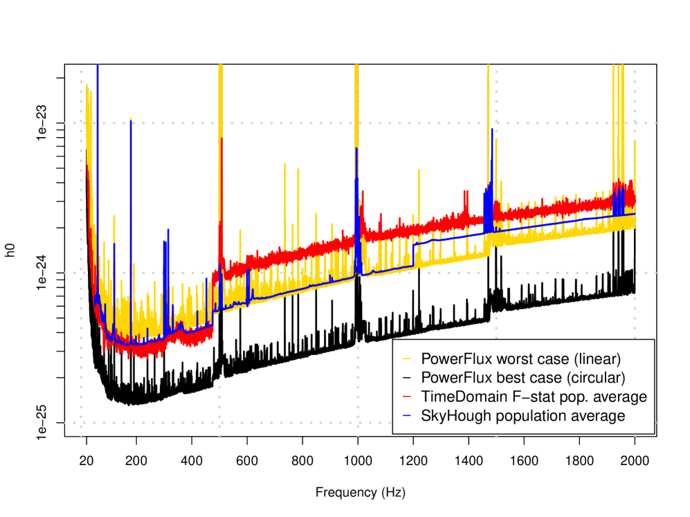
Figure 1: O1 upper limits. Looking at the right side of the plot, the upper (red) curve shows Time Domain F-statistic $95$% CL population averaged upper limits, the next lower curve (blue) shows maximum population average upper limits from SkyHough, folowed by yellow curve showing PowerFlux worst-case (linearly polarized) $95$% CL upper limits in analyzed bands. PowerFlux upper limits are maximized over sky and all intrinsic signal parameters for each frequency band displayed. The lower (black) curve shows upper limits assuming a circularly polarized source. We include the data from the low-frequency paper O1LowFreq to present the entire range 20–2000 Hz. As the computational demands grow with frequencies each pipeline tuned parameters to reduce computation load. This accounts for jumps in curves at $475$, $1200$ and $1475$ Hz. The SkyHough upper limit curve shows maximum of the range of different upper limits shown in Fig. 7 with different upper limit values corresponding to different search depths. Because of highly non-Gaussian data the SkyHough search depths are not expected to be well-estimated for each individual search band, but are representative of the noise behaviour in the entire frequency range. The data for this plot can be found in data . (color online)

II LIGO interferometers and O1 observing run

The LIGO gravitational wave network consists of two observatories, one in Hanford, Washington and the other in Livingston, Louisiana, separated by a 3000-km baseline. During the O1 run each site housed one suspended interferometer with 4 km long arms. The interferometer mirrors act as test masses, and the passage of a gravitational wave induces a differential arm length change that is proportional to the gravitational-wave strain amplitude. The Advanced LIGO ALIGODescription detectors came online in September 2015 after a major upgrade. While not yet operating at design sensitivity, both detectors reached an instrument noise 3 to 4 times lower than ever measured before in their most sensitive frequency band between 100 Hz and 300 Hz DetectorPaper .

The suspension systems of the optical elements was greatly improved, extending the usable frequency range down to 20 Hz. Use of monolithic suspensions provided for sharper resonances of so-called violin modes, resulting in narrower (in frequency) detector artifacts. An increase in mirror mass has shifted the resonances to the vicinity of 500 Hz, opening up previously-contaminated frequency bands.

With these positive effects came some new difficulties: the increase in the number of optical elements resulted in more violin modes, as well as new less well-understood resonances O1LowFreq .

Advanced LIGO’s first observing run occurred between September 12, 2015 and January 19, 2016, from which approximately 77 days and 66 days of analyzable data were produced by the Hanford (H1) and Livingston (L1) interferometers, respectively. Notable instrumental contaminants affecting the searches described here included spectral combs of narrow lines in both interferometers, many of which were identified after the run ended and mitigated for future runs. These artifacts included an 8-Hz comb in H1 with the even harmonics (16-Hz comb) being especially strong. This comb was later tracked down to digitization roundoff error in a high-frequency excitation applied to servo-control the cavity length of the Output Mode Cleaner (OMC). Similarly, a set of lines found to be linear combinations of 22.7 Hz and 25.6 Hz in the L1 data was tracked down to OMC excitation at a still higher frequency, for which digitization error occurred.

A subset of these lines with common origins at the two observatories contaminated the O1 search for a stochastic background of gravitational waves, which relies upon cross-correlation of H1 and L1 data, requiring excision of affected bands O1StochasticPaper ; O1DirectStochasticPaper ; O1LinesPaper .

Although most of these strong and narrow lines are stationary in frequency and hence do not exhibit the Doppler modulations due to the Earth’s motion expected for a CW signal from most sky locations, the lines pollute the spectrum for such sources. In sky locations near the ecliptic poles, where a putative CW signal would have little Doppler modulation, the lines contribute extreme contamination for certain signal frequencies. This effect was particularly severe for the low-frequency results in the 20–475 Hz range O1LowFreq .

III Signal waveform

In this paper we assume a standard model of a spinning non-axisymmetric neutron star. Such a neutron star radiates circularly-polarized gravitational radiation along the rotation axis and linearly-polarized radiation in the directions perpendicular to the rotation axis. For the purposes of detection and establishing upper limits the linear polarization is the worst case, as such signals contribute the smallest amount of power to the detector.

The strain signal template measured by a detector is assumed to be

$$\begin{array}[]{l}h(t)=h_{0}\left(F_{+}(t,\alpha_{0},\delta_{0},\psi)\frac{1+\cos^{2}(\iota)}{2}\cos(\Phi(t))+\right.\\ \quad\quad\quad\left.\vphantom{\frac{1+\cos^{2}(\iota)}{2}}+F_{\times}(t,\alpha_{0},\delta_{0},\psi)\cos(\iota)\sin(\Phi(t))\right)\textrm{~{},}\end{array}$$ (1)

where $F_{+}$ and $F_{\times}$ characterize the detector responses to signals with “$+$” and “$\times$” quadrupolar polarizations S4IncoherentPaper ; EarlyS5Paper ; FullS5Semicoherent , the sky location is described by right ascension $\alpha_{0}$ and declination $\delta_{0}$, the inclination of the source rotation axis to the line of sight is denoted $\iota$, and we use $\psi$ to denote the polarization angle (i.e. the projected source rotation axis in the sky plane).

The phase evolution of the signal is given by the formula

$$\Phi(t)=2\pi\left(f_{\textrm{source}}\cdot(t-t_{0})+f^{(1)}\cdot(t-t_{0})^{2}/2\right)+\phi\textrm{~{},}$$ (2)

with $f_{\textrm{source}}$ being the source frequency and $f^{(1)}$ denoting the first frequency derivative (which, when negative, is termed the spindown). We use $t$ to denote the time in the Solar System barycenter frame. The initial phase $\phi$ is computed relative to reference time $t_{0}$. When expressed as a function of local time of ground-based detectors, Equation 2 acquires sky-position-dependent Doppler shift terms.

Most natural “isolated” sources are expected to have negative first frequency derivative, as the energy lost in gravitational or electromagnetic waves would make the source spin more slowly. The frequency derivative can be positive when the source is affected by a strong slowly-variable Doppler shift, such as due to a long-period orbit.

IV PowerFlux search for continuous gravitational radiation

IV.1 Overview

This search has two main components. First, the main PowerFlux algorithm S4IncoherentPaper ; EarlyS5Paper ; FullS5Semicoherent ; PowerFluxTechNote ; PowerFlux2TechNote ; PowerFluxPolarizationNote is run to establish upper limits and produce lists of outliers with signal-to-noise ratio (SNR) greater than 5. Next, the Loosely Coherent detection pipeline loosely_coherent ; loosely_coherent2 ; FullS5Semicoherent is used to reject or confirm collected outliers.

Both algorithms calculate power for a bank of signal model templates and compute upper limits and signal-to-noise ratios for each template based on comparison to templates with nearby frequencies and the same sky location and spindown. The input time series is broken into $50$%-overlapping long segments with durations shown in Table 1, which are then Hann-windowed and Fourier-transformed. The resulting short Fourier transforms (SFTs) are arranged into an input matrix with time and frequency dimensions. The power calculation can be expressed as a bilinear form of the input matrix $\left\{a_{t,f}\right\}$:

$$P[f]=\sum_{t_{1},t_{2}}a_{t_{1},f+\delta f(t_{1})}a_{t_{2},f+\delta f(t_{2})}^{*}K_{t_{1},t_{2},f}$$ (3)

Here $\delta f(t)$ denotes the detector frame frequency drift due to the effects from both Doppler shifts and the first frequency derivative. The sum is taken over all times $t$ corresponding to the midpoint of the short Fourier transform time interval. The kernel $K_{t_{1},t_{2},f}$ includes the contribution of time-dependent SFT weights, antenna response, signal polarization parameters, and relative phase terms loosely_coherent ; loosely_coherent2 .

The main semi-coherent PowerFlux algorithm uses a kernel with main diagonal terms only that is easy to make computationally efficient. The Loosely Coherent algorithms increase coherence time while still allowing for controlled deviation in phase loosely_coherent . This is done using more complicated kernels that increase effective coherence length.

The effective coherence length is captured in a parameter $\delta$, which describes the amount of phase drift that the kernel allows between SFTs, with $\delta=0$ corresponding to a fully coherent case, and $\delta=2\pi$ corresponding to incoherent power sums.

Depending on the terms used, the data from different interferometers can be combined incoherently (such as in stage 0, see Table 1) or coherently (as used in stages 2 or 3). The coherent combination is more computationally expensive but provides much better parameter estimation.

The upper limits (Fig. 1) are reported in terms of the worst-case value of $h_{0}$ (which applies to linear polarizations with $\iota=\pi/2$) and for the most sensitive circular polarization ($\iota=0$ or $\pi$). As described in the previous paper FullS5Semicoherent , the pipeline does retain some sensitivity, however, to non-general-relativity GW polarization models, including a longitudinal component, and to slow amplitude evolution. A search for non-general-relativity GW signals from known pulsars is described in O1DirectedTensorial .

The 95% confidence level upper limits (see Fig. 1) produced in the first stage are based on the overall noise level and largest outlier in strain found for every combination of sky position, spindown, and polarization in each frequency band in the first stage of the pipeline. These bands are analyzed by separate instances of PowerFlux FullS5Semicoherent , and their widths vary depending on the frequency range (see Table 1). A followup search for detection is carried out for high-SNR outliers found in the first stage.

IV.2 Universal statistics

The improvements in detector noise for Advanced LIGO included extension of the usable band down to $\sim$20 Hz, allowing searches for lower-frequency sources than previously possible with LIGO data. As discussed above, however, a multitude of spectral combs contaminated the data, and in contrast to the 23-month S5 Science Run and 15-month S6 Science Runs of initial LIGO, the 4-month O1 run did not span the Earth’s full orbit, which means the Doppler shift magnitudes from the Earth’s motion are reduced, on the whole, compared to those of the earlier runs. In particular, for certain combinations of sky location, frequency, and spindown, a signal can appear relatively stationary in frequency in the detector frame of reference, with the effect being most pronounced for low signal frequencies as noted in O1LowFreq .

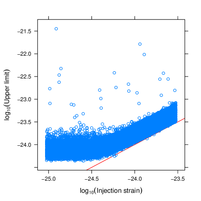
Figure 2: PowerFlux upper limit validation. Each point represents a separate injection in the 475-1475 Hz frequency range. Each established upper limit (vertical axis) is compared against the injected strain value (horizontal axis, red line). The plot for high frequency range 1475-2000 Hz is very similar and not included in this paper. (color online).

To allow robust analysis of the entire spectrum, we use in this analysis the Universal statistic algorithm universal_statistics for establishing upper limits. The algorithm is derived from the Markov inequality and shares its independence from the underlying noise distribution. It produces upper limits less than $5$% above optimal in the case of Gaussian noise. In non-Gaussian bands it can report values larger than what would be obtained if the distribution were known, but the upper limits are always at least 95% valid. Fig. 2 shows results of an injection run performed as described in FullS5Semicoherent . Correctly-established upper limits lie above the red line.

Stage	Instrument sum	Phase coherence	Spindown step	Sky refinement	Frequency refinement	SNR increase
		rad	Hz/s			%
20-475 Hz frequency range, 7200 s SFTs, 0.0625 Hz frequency bands
0	Initial/upper limit semi-coherent	NA	$1\times 10^{-10}$	$1$	$1/2$	NA
1	incoherent	$\pi/2$	$1.0\times 10^{-10}$	$1/4$	$1/8$	20
2	coherent	$\pi/2$	$5.0\times 10^{-11}$	$1/4$	$1/8$	10
3	coherent	$\pi/4$	$2.5\times 10^{-11}$	$1/8$	$1/16$	10
4	coherent	$\pi/8$	$5.0\times 10^{-12}$	$1/16$	$1/32$	7
475-1475 Hz frequency range, 3600 s SFTs, 0.125 Hz frequency bands
0	Initial/upper limit semi-coherent	NA	$1\times 10^{-10}$	$1$	$1/2$	NA
1	coherent	$\pi/2$	$3.0\times 10^{-10}$	$1/4$	$1/8$	40
2	coherent	$\pi/4$	$1.5\times 10^{-10}$	$1/8$	$1/8$	12
3	coherent	$\pi/8$	$7.5\times 10^{-11}$	$1/8$	$1/16$	0
1475-2000 Hz frequency range, 1800 s SFTs, 0.25 Hz frequency bands
0	Initial/upper limit semi-coherent	NA	$1\times 10^{-10}$	$1$	$1/2$	NA
1	coherent	$\pi/2$	$3.0\times 10^{-10}$	$1/4$	$1/8$	40
2	coherent	$\pi/4$	$1.5\times 10^{-10}$	$1/8$	$1/8$	12
3	coherent	$\pi/8$	$7.5\times 10^{-11}$	$1/8$	$1/16$	8

Table 1: PowerFlux analysis pipeline parameters. Starting with stage 1, all stages used the Loosely Coherent algorithm for demodulation. The sky and frequency refinement parameters are relative to values used in the semicoherent PowerFlux search. The 7200 s SFTs used for analysis of 20-475 Hz range were too computationally expensive for higher frequencies and smaller 3600 s and 1800 s SFTs were used instead. The breakpoints 475 Hz and 1475 Hz breakpoints were chosen so that more computationally expensive range ends just before heavy instrumental artifacts due to violin modes of mirrors and beamsplitter.

IV.3 Detection pipeline

The outlier follow-up used in FullS5Semicoherent ; S6PowerFlux has been extended with additional stages (see Table 1) to winnow the larger number of initial outliers, expected because of non-Gaussian artifacts and larger initial search space. This paper uses fewer stages than O1LowFreq because of the use of a dynamic programming algorithm which allowed to proceed straight to coherent combinations of interferometer data.

The initial stage (marked 0) scans the entire sky with a semi-coherent algorithm that computes weighted sums of powers of Hann-windowed SFTs. These power sums are then analyzed to identify high-SNR outliers. A separate algorithm uses Universal statistics universal_statistics to establish upper limits.

The entire dataset is partitioned into three stretches of approximately equal length, and power sums are produced independently for any contiguous combinations of these stretches. As in orionspur ; S6PowerFlux the outlier identification is performed independently in each contiguous combination.

High-SNR outliers are subject to a coincidence test. For each outlier with $\textrm{SNR}>7$ in the combined H1 and L1 data, we require there to be outliers in the individual detector data of the same sky area that had $\textrm{SNR}>5$, matching the parameters of the combined-detector outlier within $167$ $\mu$Hz in frequency ($333$ $\mu$Hz for the 1475–2000 Hz band), and $6\times 10^{-10}$ Hz/s in spindown. The combined-detector SNR is required to be above both single-detector SNRs.

The identified outliers using combined data are then passed to a followup stage using the Loosely Coherent algorithm loosely_coherent with progressively tighter phase coherence parameters $\delta$, and improved determination of frequency, spindown and sky location.

A new feature of this analysis is the use of a dynamic programming algorithm similar to the Viterbi method viterbimethod ; viterbi in followup stages. The three stretches are each partitioned into four parts (forming 12 parts total). Given a sequence of parts the weighted sum is computed by combining pre-computed sums for each part, but the frequency is allowed to jump by at most one sub-frequency bin. To save space, the weighted sums are maximized among all sequence combinations that have the same ending frequency bin. The use of dynamic programming made the computation efficient.

Because the resulting power sum is a maximum of many power sums, the statistics are slightly altered and are not expected to be Gaussian. They are sufficiently close to Gaussian, however, and the Universal statistic algorithm works well with this data, even though it was optimized for a Gaussian case. The followup stages use SNR produced by the same algorithm.

Allowing variation between the stretches widens the range of acceptable signals, making the search more robust. The greatest gains from this improvement, though, are in computational speed, as we can use coarser spindown steps and other parameters with only a small loss in sensitivity. This was critical to completing the Monte-Carlo simulations that verify effectiveness of the pipeline (Fig. 3).

As the initial stage 0 sums only powers, it does not use the relative phase between interferometers, which results in some degeneracy between sky position, frequency and spindown. The first Loosely Coherent followup stage combines interferometer powers coherently and demands greater temporal coherence (smaller $\delta$) , which should boost SNR of viable outiers by at least 40%. Subsequent stages provide tighter bounds on outlier location. Surviving outliers are passed to the Einstein@Home pipeline O1EH ; S6BucketFU .

The testing of the pipeline was performed by comprehensive simulations in each frequency range. Injection recovery efficiencies from simulations covering the $475$-$1475$ Hz range are shown in Fig. 3. The simulations for higher frequencies $1475$-$2000$ Hz produced a very similar plot, which is not shown here.

We want to highlight that simulations included highly contaminated regions such as violin modes and demonstrate the algorithm’s robustness to extreme data.

In order to maintain low false dismissal rates, the followup pipeline used wide tolerances in associating outliers between stages. For example, when transitioning from the semi-coherent stage 0 to the Loosely Coherent stage 1, the effective coherence length increases by a factor of 4. The average true signal SNR should then increase by more than $40$%. An additional $40$% is expected from coherent combination of data between interferometers. But the threshold used in followup is only $40$%, which accomodates unfavorable noise conditions, template mismatch, detector artifacts, and differences in detector duty cycle.

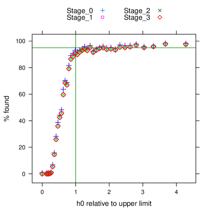
Figure 3: PowerFlux injection recovery. The injections were performed in the 475-1475 Hz band. The injected strain divided by the upper limit in this band computed without injection is shown on the horizontal axis. The percentage of surviving injections is shown on the vertical axis, with a horizontal line drawn at the $95$% level. Stage 0 is the output of the coincidence test after the initial semi-coherent search. The plot for high frequency range 1475-2000 Hz is very similar and not included here. (color online).

Our recovery criteria demand that an outlier close to the true injection location (within $3$ mHz in frequency $f$, $7\times 10^{-11}$ Hz/s in spindown and [$6$ rad$\cdot$Hz$/f$, $12$ rad$\cdot$Hz$/f$] for [$475$-$1475$ Hz, $1475$-$2000$ Hz] in sky location) be found and successfully pass through all stages of the detection pipeline. As each stage of the pipeline passes only outliers with an increase in SNR, signal injections result in outliers that strongly stand out above the background.

The followup code was verifed to recover $90$% of injections at or above the upper limit level for a uniform distribution of injection frequencies. (Fig. 3). This fraction rises with injection strength. Compared with similar PowerFlux plots in earlier papers we do not reach $95$% injection recovery right away. This is due to uneven sensitivity between interferometers (our concidence test demands an outlier be marginally seen in individual interferometers), as well as heavily contaminated data.

We note that this is still a 95% upper limit: if a louder signal had actually been present, we would have set a higher upper limit 95% of the time, even if we could only detect the signal 90% of the time.

V SkyHough search for continuous gravitational radiation

V.1 Overview

The SkyHough search method is described in detail in SkyHough1 ; SkyHough2 ; Chi2Hough ; S5Hough , and was also used in the previous low-frequency O1 search O1LowFreq . The search consists primarily of two main steps. First, the data from the two LIGO interferometers are analyzed in separate all-sky searches for continuous gravitational wave signals, using a Hough transform algorithm that produces sets of top-lists of the most significant events. In the second step, coincidence requirements on candidates are imposed.

In the first step, an implementation of the weighted Hough transform, SkyHough SkyHough2 ; S5Hough , is used to map points from the digitized time-frequency plane of the data, called the peak-gram, into the space of the source parameters. The algorithm searches for signals whose frequency evolution fits the pattern produced by the Doppler shift and spindown in the time-frequency plane of the data. In this case, the Hough number count, $n$, is the sum of the ones and zeroes of the peak-gram weighted using the detector antenna pattern and the noise level. A useful detection statistic is the significance (or critical ratio), and is given by

$$s=\frac{n-\langle n\rangle}{\sigma}\,,$$ (4)

where $\langle n\rangle$ and $\sigma$ are the expected mean and standard deviation of the Hough number count for pure noise.

The analysis of the SkyHough search presented here has not identified any convincing continuous gravitational wave signal. Hence, we proceed to set upper limits on the maximum intrinsic wave strain $h_{0}$ that is consistent with our observations for a population of signals described by an isolated triaxial rotating neutron star. As in previous searches, we set all-sky population-based frequentist upper limits, that are given in different frequency sub-bands.

V.2 Detection pipeline

As was done in the previous low-frequency Advanced-LIGO O1 search O1LowFreq , covering frequencies up to 475 Hz, this search method uses calibrated detector $h(t)$ data to create 1800 s Tukey-windowed SFTs, where each SFT is created from a segment of detector data that is at least 1800 s long. From this step, 3684 and 3007 SFTs are created for H1 and L1, respectively. SFT data from a single interferometer are analyzed by setting a threshold of 1.6 on the normalized power and then creating a peak-gram (a collection of zeros and ones). The averaged spectrum is determined via a running-median estimation S4IncoherentPaper which uses 50 frequency bins to each side of the current bin.

The SkyHough search analyzes 0.1 Hz bands over the frequency interval 475–2000 Hz, frequency time derivatives in the range $[-1.0,+0.1]\times 10^{-8}$ Hz/s, and covers the entire sky. A uniform grid spacing, equal to the size of a SFT frequency bin, $\delta f=1/T_{\textrm{\mbox{\tiny{coh}}}}=5.556\times 10^{-4}~{}\mathrm{Hz}$ is chosen, where $T_{\textrm{\mbox{\tiny{coh}}}}$ is the duration of a SFT. The resolution in the first frequency derivative, $\delta\dot{f}$, is given by the smallest value of $\dot{f}$ for which the intrinsic signal frequency does not drift by more than one frequency bin during the total observation time $T_{\textrm{\mbox{\tiny{obs}}}}$: $\delta\dot{f}=\delta f/T_{\textrm{\mbox{\tiny{obs}}}}\sim 4.95\times 10^{-11}~{}\mathrm{Hz}~{}\mathrm{s}^{-1}$. This yields 203 spin-down values and 21 spin-up values for each frequency. The angular spacing of the sky grid points, $\delta\theta$ (in radians), is frequency dependent, with the number of templates increasing with frequency, as given by equation (4.14) of Ref. SkyHough1 :

$$\delta\theta=\frac{10^{4}\,\delta f}{fN_{p}}\,,$$ (5)

where $N_{p}$ is a variable that we call pixelfactor. This variable can be manually changed to accommodate the desired sky resolution and consequently the computational cost of the search. The scaling factor of $10^{4}$ accounts for the maximum sky-position-dependent frequency modulation $v/c\sim 10^{-4}$ due to Earth’s orbit. For the Initial-LIGO S5 search $N_{p}$ was set to 0.5 S5Hough , while in the previous low-frequency Advanced-LIGO O1 search O1LowFreq $N_{p}$ was set to 2, thus increasing the sky resolution by a factor of 16.

For each 0.1 Hz frequency band, the parameter space is split further into 209 sub-regions of the sky. For every sky region and frequency band the analysis program compiles a list of the 1000 most significant candidates (those with the highest critical ratio values). A final list of the 1000 most significant candidates for each 0.1 Hz frequency band is constructed, with no more than 300 candidates from a single sky region. This procedure reduces the influence of instrumental spectral disturbances that affect specific sky regions.

As the number of sky positions in an all-sky search increases with the square of the frequency, the computational cost becomes larger for the highest frequencies. In order to perform this SkyHough all-sky search within the allocated computational budget, the search presented here is split in two different bands: from 475 to 1200 Hz, and from 1200 Hz to 2000 Hz. The pixelfactor $N_{p}$ is set equal to 2 for 475–1200 Hz band and equal to 0.5 for 1200–2000 Hz, thus performing a lower sky grid resolution search at higher frequencies. Of course, these parameter choices, duration of the SFTs, sky resolution, and size of the toplist per frequency band, have implications on the final sensitivity of the search itself compared to what could have been achieved. Around 1200 Hz we estimate that the sensitivity would have been 20% better if the pixelfactor $N_{p}$ had remained 2, as can be inferred from Fig. 7.

V.3 The post-processing stage

The post-processing of the top-lists for each 0.1 Hz band consists of the following steps:

(i) Search for coincident candidates among the H1 and L1 data sets, using a coincidence window of $d_{\rm SH}<\sqrt{14}$. This dimensionless quantity is defined as:

$$d_{\rm SH}=\sqrt{(\Delta f/\delta f)^{2}+(\Delta\dot{f}/\delta\dot{f})^{2}+(\Delta\theta/\delta\theta)^{2}}$$ (6)

to take into account the distances in frequency, spin-down and sky location with respect to the grid resolution in parameter space. Here $\Delta\theta$ is the sky angle separation. Each coincidence pair is then characterized by its harmonic mean significance value and a center in parameter space: the mean weighted value of frequency, spin-down and sky-location obtained by using their corresponding individual significance values.

(ii) The surviving coincidence pairs are clustered, using the same coincidence window of $d_{\rm SH}<\sqrt{14}$ applied to the coincidence centers. Each coincident candidate can belong to only a single cluster, and an element belongs to a cluster if there exists at least another element within that distance. Only the highest ranked cluster, if any, will be selected for each 0.1 Hz band. Clusters are ranked based on their mean significance value, but where all clusters overlapping with a known instrumental line are ranked below any cluster with no overlap. A cluster is always selected for each of the 0.1 Hz bands that had coincidence candidates. In most cases the cluster with the largest mean significance value coincides also with the one containing the highest individual value.

Clusters were marked if they overlapped with a list of known instrumental lines. To perform this veto, we consider the frequency interval derived from frequency evolution given by the $f$ and $\dot{f}$ values of the center of the cluster together with its maximum Doppler shift, and check if the resulting frequency interval overlaps with the frequency of a known line.

These steps (i)-(ii) take into account the possibility of coincidences and formation of clusters across boundaries of consecutive 0.1 Hz frequency bands.

(iii) Based on previous studies AllSkyMDC , we require that interesting clusters must have a minimum population of 2; otherwise they are discarded. This is similar to the “occupancy veto” described in BehnkePP2015 .

The remaining candidates are manually examined. In particular, outliers are also discarded if the frequency span of the cluster coincides with the list of instrumental lines described in Sec. II, or if there are obvious spectral disturbances associated with one of the detectors. Multi-detector searches, as those described in O1LowFreq , are also performed to verify the consistency of a possible signal, and surviving outliers are passed to the Einstein@Home pipeline S6BucketFU ; O1EH .

V.4 Upper limit computation

As in previous searches S5Hough ; O1LowFreq , we set a population-based frequentist upper limit at the 95% confidence level. Upper limits are derived for each 0.1 Hz band from the estimated average sensitivity depth, in a similar way to the procedure used in the Einstein@Home searches S6BucketEH ; O1EH .

For a given signal strength $h_{0}$, the sensitivity depth is defined as:

$${\mathcal{D}}:={\sqrt{S_{h}}\over h_{0}}~{}~{}[{1/\sqrt{\text{Hz}}}].$$ (7)

Here, $S_{n}$ is the maximum over both detectors of the power spectral density of the data, at the frequency of the signal. $S_{n}$ is estimated as the power-2 mean value, $\left(\sum_{i=1}^{N}\left(S^{(i)}_{k}\right)^{-2}/N\right)^{-2}$, across the different noise levels $S^{(i)}_{k}$ of the different $N$ SFTs.

Two different values of average depth are obtained for the 475–1200 Hz and 1200–2000 Hz frequency bands respectively, consistent with the change in the sky grid resolution during the search. The depth values corresponding to the averaged all-sky 95% confidence detection efficiency are obtained by means of simulated periodic gravitational wave signals added into the SFT data of both detectors H1 and L1 in a limited number of frequency bands. In those bands, the detection efficiency, i.e., the fraction of signals that are considered detected, is computed as a function of signal strength $h_{0}$ expressed by the sensitivity depth.

For the 475–1200 Hz lower-frequency band, eighteen different 0.1 Hz bands were selected with the following starting frequencies: [532.4, 559.0, 580.2, 646.4, 658.5, 678.0, 740.9, 802.4, 810.2, 865.3, 872.1, 935.7, 972.3, 976.3, 1076.3, 1081.0, 1123.4, 1186.0] Hz. These bands were chosen to be free of known spectral disturbances in both detectors, with no coincidence candidates among the H1 and L1 data sets, and scattered over the whole frequency band. In all these selected bands, we generated nine sets of 400 signals each, with fixed sensitivity depth in each set and random parameters $(f,\alpha,\delta,\dot{f},\varphi_{0},\psi,\cos\iota)$. Each signal was added into the data of both detectors, and an analysis was done using the SkyHough search pipeline over a frequency band of 0.1 Hz and the full spin-down range, but covering only one sky-patch. For this sky-patch a list of 300 loudest candidates was produced. Then we imposed a threshold on significance, based on the minimum significance found in the all-sky search in the corresponding 0.1 Hz band before any injections. The post-processing was then done using the same parameters used in the search, including the population veto. A signal was considered detected if the center of the selected cluster, if any, lay within a distance $d_{\rm SH}<13$ from the real injected value. This window was chosen based on previous studies AllSkyMDC and prevented miscounts due to noise fluctuations or artifacts.

For the 1200–2000 Hz frequency band, the following eighteen different 0.1 Hz bands were selected: [1248.7, 1310.6, 1323.5, 1334.4, 1410.3, 1424.6, 1450.2, 1562.6, 1580.4, 1583.2, 1653.2, 1663.6, 1683.4, 1704.3, 1738.2, 1887.4, 1953.4, 1991.5] Hz. The same procedure described above was applied to these bands.

Figure 4: Detection efficiency as a function of depth obtained for the 0.1 Hz frequency band starting at 580.2 Hz. Each red dot corresponds to a set of 400 signal injections and error bars on the data points represent the 2$\sigma_{E}$ standard binomial error. The (black) solid line corresponds to the fitted sigmoid curve and the (blue) shaded envelope corresponds to the $2\sigma_{F}$ calculated according to Eq. (10). The diamond shows the depth value corresponding to the 95% detection efficiency, $\mathcal{D}^{95\%}$, along with the $2\sigma_{F}$ uncertainty in black markers.

Figure 5: Depth values corresponding to the 95% detection efficiency, $\mathcal{D}^{95\%}$, obtained for 18 0.1 Hz frequency bands between 475 and 1200 Hz, along with their corresponding $2\sigma_{F}$ uncertainties from the sigmoid fit in red markers. The average of the measured depths at different frequencies being $\langle\mathcal{D}^{95\%}\rangle_{\rm Low}=20.5$ ${\text{Hz}}^{-1/2}$.

Figure 6: Depth values corresponding to the 95% detection efficiency, $\mathcal{D}^{95\%}$, obtained for 18 0.1 Hz frequency bands between 1200 and 2000 Hz, along with their corresponding $2\sigma_{F}$ uncertainties in red markers. The average of the measured depths at different frequencies being $\langle\mathcal{D}^{95\%}\rangle_{\rm High}=16.5$ ${\text{Hz}}^{-1/2}$.

Figure 7: SkyHough O1 upper limits. The solid (blue) line shows the averaged $95$% confidence level upper limits on the gravitational wave amplitude for every analyzed 0.1 Hz band. The vertical (grey) lines indicate 25 0.1 Hz bands in which outliers were found and consequently no upper limits were set. The lighter region around the upper limit represents the $7.4\%$ and $15\%$ uncertainty levels. The jump in sensitivity and uncertainty at 1200 Hz corresponds to the decrease in the sky grid resolution during the search, tuned to reduce the computational load.

We collected the results from the two sets of 18 frequency bands and for each frequency the detection efficiency $E$ versus depth $\mathcal{D}$ values were fitted to a sigmoid function of the form:

$$E(\mathcal{D})=1-\frac{1}{1+\exp(b(\mathcal{D}-a))}\,,$$ (8)

using the nonlinear regression algorithm nlinfit provided by Matlab. Since the detection rate follows a binomial distribution each data point was weighted by the standard $\sigma_{E}$ error given by

$$\sigma_{E}=\sqrt{E(1-E)\over N_{I}}\,,$$ (9)

where $N_{I}$ is the number of injections performed. From the estimated coefficients $a$ and $b$ along with the covariance matrix $C$, we estimated the $\sigma_{F}$ envelope on the fit given by

$$\sigma_{F}=\pm\sqrt{(\partial_{a}E)^{2}C_{aa}+2(\partial_{a}E)(\partial_{b}E)C_{ab}+(\partial_{b}E)^{2}C_{bb}}\,,$$ (10)

where $\partial$ indicates partial derivative, and derived the corresponding depth at the 95% detection efficiency, $\mathcal{D}^{95\%}$, as illustrated in Figure 4.

Figures 5 and 6 show the obtained depth values for each frequency corresponding to the 95% efficiency level, $\mathcal{D}^{95\%}$, together with their $2\sigma$ uncertainty $\delta\mathcal{D}^{95\%}=2\sigma_{F}$.

As representative of the sensitivity depth of the search, we took the average of the measured depths for each of the two sets of 18 different frequencies. This yielded $\langle\mathcal{D}^{95\%}\rangle_{\rm Low}=20.5$ ${\text{Hz}}^{-1/2}$ for the lower 475–1200 Hz band and $\langle\mathcal{D}^{95\%}\rangle_{\rm High}=16.5$ ${\text{Hz}}^{-1/2}$, for the higher 1200–2000 Hz band, being the range of variation observed on the measured sensitivity depth of individual frequency bands with respect to the averaged values of $7.4\%$ and $15\%$, respectively.

The 95% confidence upper limit on $h_{0}$ for undisturbed bands can then be derived by simply scaling the power spectral density of the data, $h_{0}^{95\%}=\sqrt{S_{n}}/\mathcal{D}^{95\%}$. The computed upper limits are shown in Figure 7 together with their uncertainty introduced by the estimation procedure. No limits have been placed in 25 0.1 Hz bands in which coincident candidates were detected, as this scaling procedure can have larger errors in those bands due to the presence of spectral disturbances.

VI Time domain $\mathcal{F}$-statistic  search for continuous gravitational radiation

The Time-Domain $\mathcal{F}$-statistic search method uses the algorithms described in jks ; AstoneBJPK2010 ; VSR1TDFstat ; PisarskiJ2015 and has been applied to an all-sky search of VSR1 data VSR1TDFstat and to the low frequency part of the LIGO O1 data O1LowFreq .

The main tool is the $\mathcal{F}$-statistic jks by which one can search coherently the data over a reduced parameter space consisting of signal frequency, its derivatives, and the sky position of the source. The F-statistic eliminates the need to sample over the four remaining parameters (see Eqs. 1 and 2): the amplitude $h_{0}$, the inclination angle $\iota$, the polarization angle $\psi$, and the initial phase $\phi$. Once a signal is identified the estimates of those four parameters are obtained from analytic formulae. However, a coherent search over the whole 120 days long LIGO O1 data set is computationally prohibitive and we need to apply a semi-coherent method, which consists of dividing the data into shorter time domain segments. The short time domain data are analyzed coherently with the $\mathcal{F}$-statistic. Then the output from the coherent search from time domain segments is analyzed by a different, computationally-manageable method. Moreover, to reduce the computer memory required to do the search, the data are divided into narrow-band segments that are analyzed separately. Thus our search method consists primarily of two parts. The first part is the coherent search of narrowband, time-domain segments. The second part is the search for coincidences among the candidates obtained from the coherent search. The pipeline is described in Section IV of O1LowFreq (see also Figure 13 of O1LowFreq for the flow chart of the pipeline). The same pipeline is used in the high frequency analysis except that a number of parameters of the search are different. The choice of parameters was motivated by the requirement to make the search computationally manageable.

As in the low frequency search, the data are divided into overlapping frequency bands of 0.25 Hz. As a result, the band $[475$-$2000]$ Hz has $6300$ frequency bands. The time series is divided into segments, called frames, of two sidereal days long each, instead of six sidereal days as in the low frequency search. For O1 data, which is over 120 days long, we obtain 60 time frames. Each 2-day narrowband segment contains $N=86164$ data points. The O1 data has a number of non-science data segments. The values of these bad data are set to zero. For this analysis, we choose only segments that have a fraction of bad data less than 1/3 both in H1 and L1 data. This requirement results in twenty 2-day-long data segments for each band. Consequently, we have $126000$ data segments to analyze. These segments are analyzed coherently using the $\mathcal{F}$-statistic defined by Eq. (9) of  VSR1TDFstat . We set a fixed threshold for the $\mathcal{F}$-statistic of $\mathcal{F}_{0}=16$ (in low frequency search the threshold was set to $14.5$) and record the parameters of all threshold crossings, together with the corresponding values of the signal-to-noise ratio $\rho$,

$$\rho=\sqrt{2(\mathcal{F}-2)}.$$ (11)

Parameters of the threshold crossing constitute a candidate signal.

At this first stage we also veto candidate signals overlapping with the instrumental lines identified by independent analysis of the detector data.

For the search we use a four-dimensional grid of templates (parametrized by frequency, spindown, and two more parameters related to the position of the source in the sky) constructed in Sec. 4 of PisarskiJ2015 , which belongs to the family $S_{1}$ of grids considered in PisarskiJ2015 . The grid’s minimal match is $\textrm{MM}=1/2$. It is considerably looser than in the low frequency search where the parameter MM was chosen to be $\sqrt{3}/2$. The quality of a covering of space by lattice of identical hyperspheres is expressed by the covering thickness $\theta$, which is defined as the average number of hyperspheres that contain a point in the space. In four dimensions the optimal lattice covering, i.e. having the minimum is called $A_{4}^{\star}$ and it has the thickness $\theta\cong 1.765529$. The thickness of the new loose grid equals 1.767685, which is only $\sim$0.1% larger than the

In the second stage of the analysis we search for coincidences among the candidates obtained in the coherent part of the analysis. We use exactly the same coincidence search algorithm as in the analysis of VSR1 data and described in detail in Section 8 of VSR1TDFstat . We search for coincidences in each of the bands analyzed. To estimate the significance of a given coincidence, we use the formula for the false alarm probability derived in the appendix of VSR1TDFstat . Sufficiently significant coincidences are called outliers and subjected to further investigation.

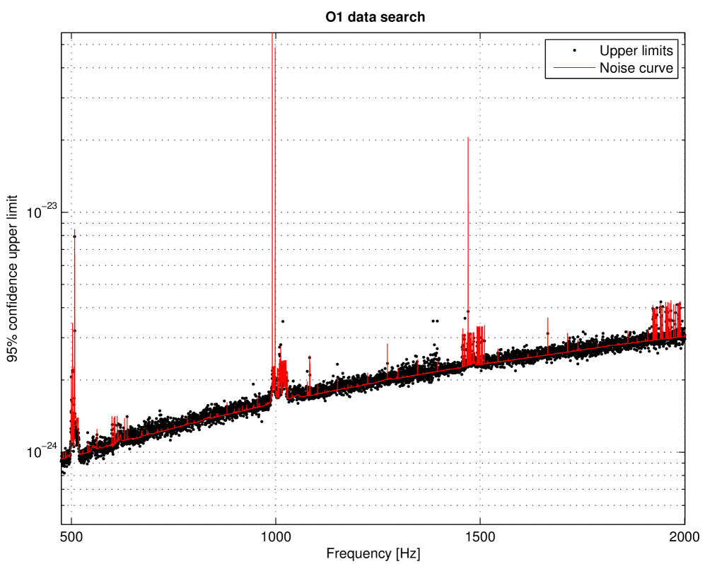
Figure 9: Time-Domain $\mathcal{F}$-statistic pipeline O1 upper limits. Black dots are the 95% confidence upper limits for each frequency, the red line denotes the H1 and L1 detectors’ average noise curve rescaled by the factor $38/\sqrt{T_{0}}$, where $T_{0}=172328$ s is the observational time of the 2-sidereal-day time series segment (color online). The factor of $38$ is larger than the factor of $27.5$ obtained the low frequency search indicating loss of sensitivity due to a looser grid of templates used here.

The sensitivity of the search is estimated by the same procedure as in the low frequency search paper (O1LowFreq , Section IV). The sensitivity is taken to be the amplitude $h_{0}$ of the gravitational wave signal that can be confidently detected. We perform the following Monte-Carlo simulations. For a given amplitude $h_{0}$, we randomly select the other seven parameters of the signal: $\omega_{0},\omega_{1},\alpha,\delta,\phi_{0},\iota$ and $\psi$. We choose frequency and spindown parameters uniformly over their range, and source positions uniformly over the sky. We choose angles $\phi_{0}$ and $\psi$ uniformly over the interval $[0,2\pi]$ and $\cos\iota$ uniformly over the interval $[-1,1]$. We add the signal with selected parameters to the O1 data. Then the data are processed through our pipeline. First, we perform a coherent $\mathcal{F}$-statistic search of each of the data segments where the signal was added. Then the coincidence analysis of the candidates is performed. The signal is considered to be detected, if it is coincident in more than 13 of the 20 time frames analyzed for a given band. We repeat the simulations one hundred times. The ratio of numbers of cases in which the signal is detected to the one hundred simulations performed for a given $h_{0}$ determines the frequentist sensitivity upper limits. We determine the sensitivity of the search in each of the 6300 frequency bands separately. The 95% confidence upper limits for the whole range of frequencies are given in Figure 9; they follow very well the noise curves of the O1 data that were analyzed. The sensitivity of our high frequency search is markedly lower than in the low frequency search. This is because here we have a shorter coherent integration time, a looser grid, and a higher threshold.

VII Search results

VII.1 PowerFlux results

The PowerFlux algorithm and Loosely Coherent method compute power estimates for gravitational waves in a given frequency band for a fixed set of templates. The template parameters include frequency, first frequency derivative and sky location. The power estimates are grouped using all parameters except frequency into a set of arrays and each array is examined separately.

Since the search target is a rare monochromatic signal, it would contribute excess power to one of the frequency bins after demodulation. The upper limit on the maximum excess relative to the nearby power values can then be established. For this analysis we use a Universal statistic universal_statistics that places conservative 95%-confidence-level upper limits for an arbitrary statistical distribution of noise power. The implementation of the Universal statistic used in this search has been tuned to provide close-to-optimal values in the common case of Gaussian distribution.

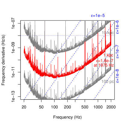
Figure 8: Range of the PowerFlux search for neutron stars spinning down solely due to gravitational radiation. This is a superposition of two contour plots. The grey and red solid lines are contours of the maximum distance at which a neutron star could be detected as a function of gravitational-wave frequency $f$ and its derivative $\dot{f}$. The dashed lines are contours of the corresponding ellipticity $\epsilon(f,\dot{f})$. The fine dotted line marks the maximum spindown searched. Together these quantities tell us the maximum range of the search in terms of various populations (see text for details) (color online).

The upper limits obtained in the search are shown in Fig. 1. The numerical data for this plot can be obtained separately data . The upper (yellow) curve shows the upper limits for a worst-case (linear) polarization when the smallest amount of gravitational energy is projected towards Earth. The lower curve shows upper limits for an optimally oriented source. Because of the day-night variability of the interferometer sensitivity due to anthropogenic noise, the upper limits for linearly polarized sources are more severely affected by detector artifacts, as the detector response to linearly polarized sources varies with the same period. We are able to establish upper limits over the entire frequency range, including bands containing harmonics of 60 Hz and violin modes.

Each point in Fig. 1 represents a maximum over the sky: only small portions of the sky are excluded, near the ecliptic poles, which are highly susceptible to detector artifacts due to stationary frequency evolution produced by the combination of frequency derivative and Doppler shifts. The exclusion procedure is described in FullS5Semicoherent and applied to $0.1$% of the sky over the entire run.

If one assumes that the source spindown is solely due to emission of gravitational waves, then it is possible to recast upper limits on source amplitude as a limit on source ellipticity. Figure 8 shows the reach of our search under different assumptions on source distance. Superimposed are lines corresponding to sources of different ellipticities.

Label	Frequency	Spindown	$\textrm{RA}_{\textrm{J}2000}$	$\textrm{DEC}_{\textrm{J}2000}$
	Hz	nHz/s	degrees	degrees
ip0	$265.575533$	$-4.15\times 10^{-3}$	$71.55193$	$-56.21749$
ip1	$848.969641$	$-3.00\times 10^{-1}$	$37.39385$	$-29.45246$
ip2	$575.163521$	$-1.37\times 10^{-4}$	$215.25617$	$3.44399$
ip3	$108.857159$	$-1.46\times 10^{-8}$	$178.37257$	$-33.4366$
ip4	$1393.540559$	$-2.54\times 10^{-1}$	$279.98768$	$-12.4666$
ip5	$52.808324$	$-4.03\times 10^{-9}$	$302.62664$	$-83.83914$
ip6	$146.169370$	$-6.73\times 10^{0\mathrm{\;\;\;}}$	$358.75095$	$-65.42262$
ip7	$1220.555270$	$-1.12\times 10^{0\mathrm{\;\;\;}}$	$223.42562$	$-20.45063$
ip8	$191.031272$	$-8.65\times 10^{0\mathrm{\;\;\;}}$	$351.38958$	$-33.41852$
ip9	$763.847316$	$-1.45\times 10^{-8}$	$198.88558$	$75.68959$
ip10	$26.341917$	$-8.50\times 10^{-2}$	$221.55565$	$42.87730$
ip11	$31.424758$	$-5.07\times 10^{-4}$	$285.09733$	$-58.27209$
ip12	$38.477939$	$-6.25\times 10^{0\mathrm{\;\;\;}}$	$331.85267$	$-16.97288$
ip13	$12.428001$	$-1.00\times 10^{-2}$	$14.32394$	$-14.32394$
ip14	$1991.092401$	$-1.00\times 10^{-3}$	$300.80284$	$-14.32394$

Table 2: Parameters of the hardware-injected simulated continuous-wave signals during the O1 data run (epoch GPS $1130529362$). Because the interferometer configurations were largely frozen in a preliminary state after the first discovery of gravitational waves from a binary black hole merger, the hardware injections were not applied consistently. There were no injections in the H1 interferometer initially, and the initial injections in the L1 interferometer used an actuation method with significant inaccuracies at high frequencies.

The detection pipeline produced 31 outliers located in the 1000–1033 Hz region heavily contaminated with violin modes (Table A), 134 outliers spanning only one data segment (about 1 month) that are particularly susceptible to detector artifacts (Tables A and A), and 48 outliers (Table A) that do not fall into either of those two categories. Each outlier is identified by a numerical index. We report SNR, frequency, spindown and sky location.

The “Segment” column describes the persistence of the outlier through the data, and specifies which contiguous subset of the three equal partitions of the timespan contributed most significantly to the outlier: see orionspur for details. A true continuous signal from an isolated source would normally have [0,2] in this column (similar contribution from all 3 segments), or on rare occasions [0,1] or [1,2]. Any other range is indicative of a statistical fluctuation, an artifact or a signal that does not conform to the phase evolution of Equation 2.

During the O1 run several simulated pulsar signals were injected into the data by applying a small force to the interferometer mirrors with auxiliary lasers. Several outliers were due to such hardware injections (Table 2).

The recovery of the hardware injections gives us additional confidence that no potential signal was missed. Manual followup has shown non-injection outliers spanning all three segments to be caused by pronounced detector artifacts. Outlier number 72 in Table A spanning two segments was also investigated with a fully coherent followup based on the Einstein@Home pipeline S6BucketFU ; O1EH . No outlier was found to be consistent with the astrophysical signal model.

VII.2 SkyHough results

In this section we report the main results of the O1 all-sky search between 475 and 2000 Hz using the SkyHough pipeline, as described in section V. In total, 71 0.1 Hz bands contained coincidence candidates: 19 in the 475–1200 Hz band, analysed with higher sky resolution, and 52 in the 1200–2000 Hz band, analysed with lower sky resolution.

After discarding all the clusters containing only one coincidence pair, this list was reduced to 25 outliers, 17 in the low frequency band and 8 in the high frequency band, which were further inspected. A detailed list of these remaining outliers is shown in Table 9. Among the 25 outliers, 17 were related to known line artifacts contaminating either H1 or L1 data and 7 were identified with the hardware injected pulsars ip1, ip2, ip7 and ip9.

Label	$s_{mean}$	Frequency	Spin-down	$\alpha$	$\delta$
		[Hz]	[nHz/s]	[deg]	[deg]
ip2	30.50	575.1635 (0.0001)	0.0170 (0.0171)	215.1005 (0.1557)	3.0138 (0.4302)
ip9	35.85	763.8507 (0.0034)	$-$0.5567 (0.5567)	203.8965 (5.0109)	73.8445 (1.8451)
ip1	36.06	848.9657 (0.0053)	0.5497 (0.2497)	37.7549 (0.3611)	$-$25.2883 (4.1642)
ip7	41.61	1220.5554 (0.0009)	0.5482 (0.5718)	229.2338 (5.8082)	4.1538 (24.6044)

Table 3: SkyHough hardware injection cluster information. The table provides the frequency, spin-down and sky location of the cluster center related to each of the hardware injections found by the SkyHough search. In parentheses the distance from the cluster center to the injected values are shown. Frequencies are converted to epoch GPS 1125972653.

Table 3 presents the parameters of the center of the clusters obtained related to these hardware injections. Two hardware injection were not recovered. Ip4 was not found since its spin-down was outside the search range, and ip14 was linearly polarized and had a strain amplitude $h_{0}$ below our sensitivity.

The only unexplained outlier around 715.7250 Hz, corresponding to Idx=6 in Table 9, was further investigated. A multi-detector Hough search was performed to verify the consistency of a possible signal. In this case the maximum combined significance obtained was $5.98$ while we would have expected a minimum value of $8.21$ in case of a real signal. The outlier was also followed up with the Einstein@Home pipeline S6BucketFU using coherent integration times of 210 and 500 hours. This search covered signal frequencies in the range $[715.724,715.726]$ Hz (epoch GPS 1125972653), frequency derivatives over $[-2.2,-1.9]\times 10^{-9}$ Hz/s, and a sky region RA = $1.063\pm 0.020$ rad, DEC = $-0.205\pm 0.020$ rad that included the whole associated cluster. This search showed that this candidate was not interesting and had a very low probability of having astrophysical origin.

Therefore, this SkyHough search did not find any evidence of a continuous gravitational wave signal. Upper limits have been computed in each 0.1 Hz band, except for the 25 bands in which outliers were found.

Label	FA	Frequency [Hz]	Spin-down [nHz/s]	$\alpha$ [deg]	$\delta$ [deg]
ip1	0	848.9687 (0.0007)	-2.4474 (2.1474)	39.4542 (2.0603)	$-$39.4354 (9.9830)
ip2	0	575.1638 (0.0003)	0.0162 (0.0163)	203.8658 (11.3903)	$-$27.1485 (30.5924)
ip4	0	1393.5286 (0.0021)	$-$24.901 (0.5991)	281.4735 (1.4858)	$-$13.3001 (0.8340)
ip7	0	1220.5540 (0.0007)	$-$0.0784 ($-$1.0416)	218.8902 (4.5354)	$-$32.1127 (11.6621)
ip9	0	763.8472 (0.0001)	$-$0.0503 (0.0503)	197.8817 (1.0039)	75.9108 (0.2212)

Table 4: Hardware injection recovery with the Time-Domain $\mathcal{F}$-statistic pipeline. The values in parentheses are the absolute errors, that is, the difference with respect to the injection parameters. Frequencies are converted to epoch GPS 1131082120.

VII.3 Time domain $\mathcal{F}$-statistic results

In the $[475,2000]$ Hz bandwidth range under study, 6300 0.25-Hz wide bands were analyzed. Vetoing candidates around the known interference lines, a certain fraction of the bandwidth was not analyzed. As a result 26% of the $[475,2000]$ Hz band was vetoed, overall.

Of 6300 bands analyzed, 307 bands were completely vetoed because of the line artifacts. As a result, the search was performed in the remaining 5993 bands. As twenty 2-days segments have been chosen for the analysis, the 119860 data segments were analyzed coherently with the $\mathcal{F}$-statistic. From the coherent search we obtained around $8.6\times 10^{10}$ candidates. These candidates were subject to a search for initial coincidences in the second stage of the Time-Domain $\mathcal{F}$-statistic analysis. The search for coincidences was performed in all the bands except for the above-mentioned 307 that were completely vetoed. In the coincidence analysis, for each band, the coincidences among the candidates were searched in twenty 2-day long time frames. In Figure 10 the results of the coincidence search are presented. The top panel shows the maximum coincidence multiplicity for each of the bands analyzed. The maximum multiplicity is an integer that varies from 3 to 20 because we require coincidence multiplicity of at least 3, and 20 is the number of time frames analyzed.

Figure 10: Results of Time-Domain $\mathcal{F}$-statistic pipeline coincidences as a function of the band frequency. Top panel: maximum coincidence multiplicity. Bottom panel: false alarm probability for the coincidence with the maximum multiplicity.

The bottom panel of Fig. 10 shows the results for the false alarm probability of coincidence for the coincidence with the maximum multiplicity. This false alarm probability is calculated using the formula from the Appendix of VSR1TDFstat .

We define outliers as those coincidences with false alarm probabilities less than $0.1$% This criterion was adopted in our Virgo data search VSR1TDFstat and also in one of Einstein@Home searches  S4IncoherentPaper . From the analysis we have excluded bands highly perturbed by violin modes and their harmonics. Thus the following four bands were vetoed: $[500,509]$ Hz, $[1001,1025]$ Hz, $[1483,1511]$ Hz, and $[1957,1966]$ Hz. As a result we obtained 74 outliers. The parameters of these outliers are listed in Table A. The parameters of a given coincidence are calculated as the mean values of the parameters of the candidates that enter a given coincidence. Among the 74 outliers, 10 are identified with the hardware injections. Table 4 presents the estimated parameters obtained for these hardware injections, along with the absolute errors of the reconstructed parameters (the differences with respect to the injected parameters). The remaining 64 outliers include 10 that are seen only in H1 data, 1 in only the L1 data. 3 of the outliers are absent in the last one third of the data, 1 present in the first one third of the data, and 2 have a wandering frequency that increases in the first third of the run, is constant in the second third, decreases in the last one third of the run. The remaining 47 outliers seem to be harmonics of the same interference in the data. The distribution of the $\mathcal{F}$-statistic in a given time frame has approximately the same morphology for all the harmonics. The outliers are present both in H1 and L1 but not always in coincidence. When they are present in both detectors their SNRs are not consistent, and are at times much louder in L1. Moreover the outliers appear in the stretch of a two day data segment where 87% of data are zeros. The remaining data in that segment are mainly a noise free modulated periodic signal. We conclude that the interference originates from the detectors themselves as it clearly appears in a stretch of data with a small fraction of science data. Consequently no credible gravitational wave candidates were found.

VIII Conclusions

We have performed the most sensitive all-sky search to date for continuous gravitational waves in the range 475-2000 Hz using three different methods. We explored both positive and negative spindowns and placed upper limits on expected and unexpected sources. Figure 1 shows a summary of the strain amplitude upper limits obtained for the three pipelines. One pipeline (PowerFlux) presents strict all-sky limits for circular-polarization and linear polarisation sources. The other two pipelines (SkyHough and Time-Domain $\mathcal{F}$-statistic ) present frequentist population-averaged limits over the full sky and source polarisation.

At the highest frequencies we are sensitive to neutron stars with an equatorial ellipticity as small as $1.8\times 10^{-7}$ and as far away as $1$ kpc for favorable spin orientations. The maximum ellipticity a neutron star can theoretically support is at least $1\times 10^{-5}$ according to crust_limit ; crust_limit2 . Our results exclude such maximally deformed pulsars above a $200$ Hz stellar rotation frequency ($400$ Hz gravitational frequency) within $1$ kpc.

Outliers from the initial stages of each search method were meticulously followed up, but no candidates from any search survived scrutiny.

The use of the Universal statistic and Loosely Coherent algorithms allowed us to establish upper limits and achieve good detection efficiency (relative to the upper limit) in all frequency ranges, including highly contaminated areas.

SkyHough pipeline added a viewpoint of robust Hough algorithm. Although the decrease in the sky grid resolution at 1200 Hz, tuned to reduce computational load, produced a jump in sensitivity of about 20 %, this method offers an independent check of the other results. Future searches will use longer SFT time duration to allow the attainment of sensitivity close to PowerFlux at a reduced computational cost.

The use of a shorter coherent time and a looser grid for Time-Domain $\mathcal{F}$-statistic pipeline in the high frequency search with respect to the low frequency search resulted in loss of sensitivity by a factor of 3. With an increasing available computing power the search of the next data set will be performed with a considerably longer coherent time that should results in a sensitivity slightly better than the worse case for the PowerFlux analysis.

Appendix A Outlier tables

PowerFlux outliers passing all stages of automated followup from 475-2000 Hz band are separated into four tables. Table A shows all outliers spanning 2 or more segments and outside heavily contaminated frequency range 1000-1033 Hz. Table A shows outliers inside the contaminated region 1000-1033 Hz. Lastly tables A and A show “short” outliers using only 1 segment (approximately a month) of data. Table A shows such short outliers below 1100 Hz, while table A lists short outliers above 1100 Hz. The splitting frequency of 1100 Hz was chosen only to put similar numbers of outliers in each table.

Idx	SNR	Segment	Frequency	Spindown	$\textrm{RA}_{\textrm{J}2000}$	$\textrm{DEC}_{\textrm{J}2000}$	Description
			Hz	nHz/s	degrees	degrees
$3$	$3886$	$[0,2]$	$1220.55536$	$-0.300$	$229.053$	$-2.107$	Injection 7, very different H1 and L1 sensitivities
$4$	$456$	$[1,2]$	$848.97002$	$-0.350$	$37.141$	$-29.612$	Injection 1, L1 much more sensitive than H1
$5$	$375$	$[1,2]$	$763.84713$	$0.000$	$198.171$	$75.664$	Injection 9, loud enough to be visible in background of H1 and L1.
$6$	$286$	$[0,2]$	$575.16361$	$0.000$	$215.370$	$3.558$	Injection 2, L1 is more sensitive than H1
$14$	$126$	$[0,1]$	$1080.00097$	$0.200$	$271.159$	$66.681$	Exceptionally strong coincident bin-centered lines at 1080 Hz.
$16$	$85$	$[0,2]$	$1487.98795$	$-9.550$	$144.132$	$-66.819$	Strong bin-centered line in H1 at 1488.00 Hz
$19$	$68$	$[0,2]$	$1220.43752$	$-1.975$	$169.199$	$-0.960$	Induced by injection 7.
$24$	$41$	$[1,2]$	$767.96349$	$1.475$	$118.599$	$78.067$	Strong bin-centered line in H1 at 768 Hz
$25$	$37$	$[1,2]$	$615.00752$	$-4.700$	$202.130$	$63.562$	Strong broad line in L1
$26$	$37$	$[0,1]$	$713.38012$	$-3.900$	$223.547$	$64.304$	Strong bin-centered line in L1 at 713.400 Hz
$27$	$36$	$[1,2]$	$585.38340$	$-9.550$	$207.405$	$0.724$	Strong bin-centered line in L1 at 585.400 Hz
$31$	$29$	$[0,2]$	$1220.46981$	$-7.650$	$177.333$	$53.647$	Induced by injection 7.
$32$	$29$	$[0,1]$	$943.98085$	$1.250$	$341.520$	$70.413$	Strong bin-centered line in H1 at 944.00 Hz
$33$	$28$	$[0,2]$	$910.06257$	$1.475$	$100.432$	$80.276$	Strong broad line in H1
$34$	$27$	$[0,1]$	$980.41316$	$0.425$	$68.498$	$19.939$	Strong bin-centered line in L1 at 980.500 Hz, line in H1
$35$	$26$	$[0,1]$	$1457.59127$	$0.900$	$5.161$	$22.809$	Highly non-stationary L1 data
$36$	$26$	$[0,2]$	$767.97611$	$-4.025$	$106.321$	$-57.243$	Bin-centered line in H1 at 768.00 Hz
$37$	$26$	$[0,2]$	$1255.99635$	$-1.725$	$100.106$	$-67.630$	Line in H1 at 1256 Hz
$40$	$23$	$[1,2]$	$1456.03964$	$-1.600$	$215.391$	$-69.386$	Highly non-stationary H1 data, line at 1456.00 Hz
$41$	$23$	$[0,1]$	$2000.00108$	$-4.275$	$146.821$	$-64.950$	Line in H1, violin mode harmonic region
$42$	$23$	$[0,1]$	$831.94019$	$-7.550$	$139.056$	$-28.186$	Bin-centered line in H1 at 832.00 Hz
$43$	$22$	$[0,1]$	$918.82255$	$-1.525$	$294.016$	$-66.661$	Strong broad line in L1
$44$	$21$	$[0,2]$	$899.29679$	$1.475$	$298.627$	$26.700$	Strong broad line in H1
$45$	$21$	$[1,2]$	$968.29014$	$-7.550$	$105.510$	$-69.138$	Mismatch in SNR between H1 and L1
$46$	$21$	$[0,1]$	$943.94642$	$-6.450$	$72.434$	$-43.175$	Bin-centered line in H1 at 944.00 Hz
$47$	$20$	$[0,2]$	$1167.94911$	$1.325$	$81.001$	$-36.869$	Bin-centered line in H1 at 1168.00 Hz
$48$	$20$	$[0,1]$	$1983.05344$	$-4.350$	$28.614$	$-29.172$	Line in L1 at 1983.0994 Hz
$49$	$20$	$[0,2]$	$1393.47837$	$-0.075$	$269.418$	$-38.074$	Appears to be associated with injection 4
$50$	$20$	$[1,2]$	$559.75418$	$-4.975$	$99.663$	$2.943$	Bin-centered line in L1 at 559.800 Hz
$51$	$18$	$[0,1]$	$1471.00891$	$-0.600$	$19.261$	$82.386$	Highly non-stationary H1 spectrum
$52$	$18$	$[1,2]$	$629.87432$	$-4.025$	$208.388$	$61.733$	Strong broad line in L1
$53$	$17$	$[0,1]$	$918.73177$	$1.325$	$77.766$	$-40.562$	Strong broad line in L1
$54$	$17$	$[1,2]$	$623.96957$	$-0.075$	$198.261$	$63.320$	Bin-centered line in H1 at 624.00 Hz
$55$	$17$	$[1,2]$	$588.29660$	$-2.325$	$20.174$	$63.144$	Strong bin-centered line in L1 at 588.300 Hz
$57$	$17$	$[0,1]$	$1455.93002$	$-1.075$	$72.852$	$-37.095$	Very non-stationary H1 spectrum, line at 1456.00 Hz
$58$	$17$	$[0,1]$	$567.99073$	$0.525$	$275.690$	$77.944$	Strange coincident lines at 568.00 Hz
$59$	$16$	$[1,2]$	$906.51613$	$-5.650$	$114.204$	$7.807$	Bin-centered line in L1 at 906.600 Hz
$60$	$16$	$[0,2]$	$588.31398$	$-5.550$	$208.182$	$-49.133$	Strong bin-centered line in L1 at 588.300 Hz
$62$	$16$	$[0,1]$	$1400.00418$	$0.675$	$85.821$	$-67.453$	Bin-centered line in H1 at 1400.00 Hz
$63$	$16$	$[0,2]$	$575.09743$	$-10.525$	$223.480$	$54.438$	Induced by injection 2
$64$	$15$	$[1,2]$	$1055.67464$	$-8.850$	$52.210$	$-62.000$	Poor coherence between H1 and L1
$65$	$15$	$[0,2]$	$918.75333$	$-4.250$	$259.272$	$65.613$	Strong broad line in L1
$66$	$14$	$[0,1]$	$600.00424$	$-5.950$	$194.962$	$-83.060$	Strong line in H1 near 600 Hz
$67$	$14$	$[0,1]$	$906.72776$	$-4.475$	$95.914$	$8.234$	Strong broad line in H1
$68$	$13$	$[1,2]$	$1198.55097$	$1.175$	$197.933$	$80.202$	Strong broad line in H1
$69$	$13$	$[0,2]$	$627.89160$	$-8.200$	$225.017$	$32.253$	Bin-centered line in L1 at 627.900 Hz
$71$	$12$	$[1,2]$	$966.05168$	$-5.725$	$290.296$	$45.961$	H1 and L1 SNR inconsistent
$72$	$12$	$[0,1]$	$956.52184$	$-5.950$	$96.516$	$6.398$

Table 5: Outliers that passed the PowerFlux detection pipeline spanning more than one segment and excluding the 1000-1033 Hz region heavily contaminated with violin modes. Only the highest-SNR outlier is shown for each 0.1 Hz frequency region. Outliers marked with “line” had strong narrowband disturbances identified near the outlier location. Outliers marked as “non Gaussian” were identified as having non Gaussian statistics in their power sums, often due to a very steeply sloping spectrum. Segment column reports the set of contiguous segments of the data that produced the outlier, as described in VII. Frequencies are converted to epoch GPS $1130529362$.

Table 6: Outliers below 1100 Hz that passed the PowerFlux detection pipeline spanning only one segment, excluding 1000-1033 Hz region heavily contaminated with violin modes. Only the highest-SNR outlier is shown for each 0.1 Hz frequency region. Segment column reports the set of contiguous segments of the data that produced the outlier, as described in VII. Frequencies are converted to epoch GPS $1130529362$.

Table 7: Outliers above 1100 Hz that passed the PowerFlux detection pipeline spanning only one segment. Only the highest-SNR outlier is shown for each 0.1 Hz frequency region. Segment column reports the set of contiguous segments of the data that produced the outlier, as described in VII. Frequencies are converted to epoch GPS $1130529362$.

Table 8: PowerFlux outliers in 1000-1033 Hz region heavily contaminated with violin modes. Only the highest-SNR outlier is shown for each 0.1 Hz frequency region. Outliers marked with “line” had strong narrowband disturbances identified near the outlier location. Outliers marked as “non Gaussian” were identified as having non Gaussian statistics in their power sums, often due to a very steeply sloping spectrum. Segment column reports the set of contiguous segments of the data that produced the outlier, as described in VII. Frequencies are converted to epoch GPS $1130529362$.

Table 9 shows the parameters of the final 25 outliers from the SkyHough pipeline, along with comments on their likely origin. None of these outliers show evidence of being a credible gravitational wave signal.

Idx	Frequency	$\alpha$	$\delta$	Spin-down	$s_{\textrm{mean}}$	$\#_{\textrm{cluster}}$	$\#_{\textrm{L1}}$	$\#_{\textrm{H1}}$	$s^{*}_{\textrm{L1}}$	$s^{*}_{\textrm{H1}}$	$s_{\textrm{max}}$	Description
	[Hz]	[rad]	[rad]	[nHz/s]
1	501.6000	-1.4445	1.2596	0.9374	10.66	5	2	3	11.31	89.18	10.71	Quad violin mode 1st harmonic region (H1 & L1)
2	511.9968	-1.4218	1.2070	0.6773	16.31	4927	298	226	10.47	101.36	18.73	Quad violin mode 1st harmonic region (H1 & L1)
3	512.0027	1.7085	-1.1996	-0.6071	16.33	3007	245	246	11.20	101.55	18.85	Quad violin mode 1st harmonic region (H1 & L1)
4	568.0011	1.5942	-1.1783	-0.1839	7.18	3867	415	125	8.82	9.81	9.05	8 Hz comb (H1 & L1)
5	575.1635	-2.5290	0.0526	0.0170	30.50	1974	275	78	46.66	26.54	33.75	Hardware injection ip2
6	715.7250	1.0629	-0.2049	-2.0400	5.48	5	3	4	6.53	6.50	5.53	Unknown
8	763.8507	-2.7245	1.2888	-0.5567	35.85	6064	297	91	41.29	43.43	42.33	Hardware injection ip9
9	763.9016	-2.1715	0.9109	-7.1318	18.19	611	151	56	17.45	22.99	19.84	Hardware injection child ip9
11	824.0035	1.6679	-1.1996	-0.7762	7.56	1111	81	123	8.09	10.83	8.43	8 Hz comb (H1 & L1)
12	848.9657	0.6589	-0.4414	0.5497	36.06	5329	342	117	48.63	37.64	42.17	Hardware injection ip1
13	849.0020	0.4565	-0.6807	-4.0716	25.19	1983	331	108	31.08	29.57	29.35	Hardware injection child ip1
14	895.9988	-1.5481	1.1744	0.2368	10.33	244	35	79	6.48	69.62	11.45	8 Hz comb (H1 & L1)
15	952.0018	1.5957	-1.1797	-0.3216	18.57	4353	355	189	18.36	27.59	21.86	8 Hz comb (H1 & L1)
16	952.1017	-0.3965	-1.3294	-9.8134	9.08	416	138	62	9.17	15.29	9.98	8 Hz comb (H1 & L1)
17	1079.9981	-1.5517	1.1798	0.3367	22.98	2639	402	129	51.28	17.88	25.90	8 Hz comb (H1 & L1)
18	1080.0022	1.6073	-1.1825	-0.4562	22.95	5276	428	172	52.66	17.84	25.89	8 Hz comb (H1 & L1)
19	1080.1007	-0.2290	-1.3906	-9.9428	10.79	451	117	49	20.45	9.52	12.60	8 Hz comb (H1 & L1)
21	1220.5492	-2.2823	0.0725	0.5482	34.69	291	63	43	66.56	37.98	48.10	Hardware injection ip7
22	1220.7094	-1.6804	-0.5910	-9.6702	6.14	17	12	11	7.37	8.32	6.58	Hardware injection child ip7
44	1475.0997	1.5636	-1.1725	-0.0308	10.87	42	8	19	6.64	77.42	11.72	Quad violin mode 3rd harmonic region (H1 & L1)
45	1482.5000	-2.8976	1.0123	0.7317	9.04	2	1	2	6.58	51.78	9.05	Quad violin mode 3rd harmonic region (H1 & L1)
46	1487.8976	1.8780	1.1717	-1.7738	6.69	2	1	2	6.53	10.19	6.75	Quad violin mode 3rd harmonic region (H1)
66	1903.9302	-1.8796	1.5402	0.1383	15.51	65	28	12	35.47	39.89	35.48	8 Hz comb (H1 & L1)
67	1904.0020	1.5885	-1.1737	-0.4096	29.00	4779	340	141	34.94	40.65	36.82	8 Hz comb (H1 & L1)
68	1904.1028	0.9560	-1.3834	-10.0406	15.11	925	194	51	16.36	24.82	19.12	8 Hz comb (H1 & L1)

Table 9: SkyHough pipeline outliers in the range of frequencies between 475 and 2000 Hz after the population veto. The table provides the frequency, spin-down and sky location of the cluster centers found by the SkyHough search. $\#_{cluster}$ is the size of the cluster in terms of number of coincident pairs, $s_{max}$ and $s_{mean}$ are the maximum and mean value of the cluster significance, $\#_{L1}$ and $\#_{H1}$ are the number of different candidates producing coincidence pairs from the different data sets, and $s^{*}_{L1}$ and $s^{*}_{H1}$ are the maximum significance values obtained by analysing the data from H1 and L1 separately. Frequencies are converted to epoch GPS 1125972653.

Table A presents the parameters of the final 74 outliers from the Time-Domain $\mathcal{F}$-statistic pipeline, along with comments on their likely causes. None is a credible gravitational wave signal.

Table 10: Time-Domain $\mathcal{F}$-statistic pipeline outliers in the range of frequencies between 475 and 2000 Hz. The columns provide outliers false alarm probability (FAP) as well as the nominal frequencies and frequency derivatives, right ascensions and declinations found for the outliers, along with comments indicating the likely sources of the outliers. Outliers described as ”harmonics of a detector interference” are harmonics of an interference present in the detectors data when no science data are taken.

References

- (1)
- (2) Advanced LIGO, J. Aasi et al. (LIGO Scientific Collaboration), Class. Quantum Grav. 32 7 (2015)
- (3) Setting upper limits on the strength of periodic gravitational waves from PSR J1939+213, B. P. Abbott et al.(LIGO Scientific Collaboration), Phys. Rev. D 69, 082004 (2004).
- (4) Limits on Gravitational-Wave Emission from Selected Pulsars Using LIGO Data B. P. Abbott et al. (LIGO Scientific Collaboration), M. Kramer, and A. G. Lyne, Phys. Rev. Lett. 94, 181103 (2005).
- (5) Upper limits on gravitational wave emission from 78 radio pulsars B. P. Abbott et al. (LIGO Scientific Collaboration), M. Kramer, and A. G. Lyne, Phys. Rev. D 76, 042001 (2007).
- (6) Beating the spin-down limit on gravitational wave emission from the Crab pulsar, B. P. Abbott et al. (LIGO Scientific Collaboration), Astrophys. J. Lett. 683, 45 (2008).
- (7) Searches for gravitational waves from known pulsars with S5 LIGO data, B. P. Abbott et al.(LIGO Scientific Collaboration and Virgo Collaboration), Astrophys. J. 713, 671 (2010).
- (8) Results of the deepest Einstein@Home search for continuous gravitational waves from CasA from the S6 LIGO Science Run, S. J. Zhu et al. , Phys. Rev. D 94, 082008 (2016).
- (9) First search for gravitational waves from the youngest known neutron star, J. Abadie et al. (LIGO Scientific Collaboration), Astrophys. J. 722, 1504 (2010).
- (10) Searches for continuous gravitational waves from nine young supernova remnants J. Aasi et al. (LIGO Scientific Collaboration and Virgo Collaboration), Astroph. J. 813 1 (2015).
- (11) Search for continuous gravitational waves from neutron stars in globular cluster NGC 6544, B. P. Abbott et al. (LIGO Scientific Collaboration and Virgo Collaboration), submitted to Phys. Rev. D, arXiv:1607.02216, July 2016.
- (12) Searches for periodic gravitational waves from unknown isolated sources and Scorpius X-1: Results from the second LIGO science run, B. P. Abbott et al. (LIGO Scientific Collaboration), Phys. Rev. D 76, 082001 (2007).
- (13) First all-sky upper limits from LIGO on the strength of periodic gravitational waves using the Hough transform, B. P. Abbott et al. (LIGO Scientific Collaboration), Phys. Rev. D 72, 102004 (2005).
- (14) All-sky search for periodic gravitational waves in LIGO S4 data, B. P. Abbott et al. (LIGO Scientific Collaboration), Phys. Rev. D 77, 022001 (2008).
- (15) Einstein@Home search for periodic gravitational waves in LIGO S4 data, B. P. Abbott et al. (LIGO Scientific Collaboration), Phys. Rev. D 79, 022001 (2009).
- (16) All-sky LIGO Search for Periodic Gravitational Waves in the Early S5 Data, B. P. Abbott et al. (LIGO Scientific Collaboration), Phys. Rev. Lett. 102, 111102 (2009).
- (17) Einstein@Home search for periodic gravitational waves in early S5 LIGO data, B. P. Abbott et al. (LIGO Scientific Collaboration), Phys. Rev. D 80, 042003 (2009).
- (18) All-sky Search for Periodic Gravitational Waves in the Full S5 Data, B. P. Abbott et al. (The LIGO and Virgo Scientific Collaboration), Phys. Rev. D 85, 022001 (2012).
- (19) Einstein@Home all-sky search for periodic gravitational waves in LIGO S5 data, B. P. Abbott et al. (LIGO Scientific Collaboration), Phys. Rev. D 87, 042001 (2013).
- (20) Results of an all-sky high-frequency Einstein@Home search for continuous gravitational waves in LIGO 5th Science Run, A. Singh et al. , Phys. Rev. D 94 (2016) no.6, 064061.
- (21) Comprehensive All-sky Search for Periodic Gravitational Waves in the Sixth Science Run LIGO Data J. Aasi et al. (LIGO Scientific Collaboration and Virgo Collaboration), Phys. Rev. D 94, 042002 (2016).
- (22) Results of the deepest all-sky survey for continuous gravitational waves on LIGO S6 data running on the Einstein@Home volunteer distributed computing project, B. P. Abbott et al. (LIGO Scientific Collaboration and Virgo Collaboration), Phys. Rev. D 94 (2016) no.10, 102002.
- (23) First low frequency all-sky search for continuous gravitational wave signals, J. Aasi et al. (LIGO Scientific Collaboration and Virgo Collaboration), Phys. Rev. D 93, 042007 (2016).
- (24) A search of the Orion spur for continuous gravitational waves using a ”loosely coherent” algorithm on data from LIGO interferometers J. Aasi et al. (LIGO Scientific Collaboration and Virgo Collaboration), Phys. Rev. D 93, 042006 (2016).
- (25) Application of a Hough search for continuous gravitational waves on data from the 5th LIGO science run, J. Aasi et al. (LIGO Scientific Collaboration and Virgo Collaboration), Class. Quantum Grav. 31, 085014 (2014).
- (26) Implementation of an -statistic all-sky search for continuous gravitational waves in Virgo VSR1 data, J. Aasi et al. (LIGO Scientific Collaboration and Virgo Collaboration), Class. Quantum Grav. 31, 165014 (2014)
- (27) First search for gravitational waves from known pulsars with Advanced LIGO B.P. Abbott, Benjamin P. et al. ( LIGO Scientific and Virgo Collaborations) Astrophys.J. 839 (2017) no.1, 12, Erratum: Astrophys.J. 851 (2017) no.1, 71
- (28) Directional Limits on Persistent Gravitational Waves from Advanced LIGO’s First Observing Run, B. P. Abbott et al. (LIGO Scientific Collaboration and Virgo Collaboration), Phys. Rev. Lett. 118, 121102 (2017).
- (29) First low-frequency Einstein@Home all-sky search for continuous gravitational waves in Advanced LIGO data, B. P. Abbott et al. (LIGO Scientific Collaboration and Virgo Collaboration), Phys. Rev. D 96, 122004 (2017)
- (30) All-sky Search for Periodic Gravitational Waves in the O1 LIGO Data, B. P. Abbott et al. (LIGO Scientific Collaboration and Virgo Collaboration), Phys. Rev. D 96, 062002 (2017)
- (31) On blind searches for noise dominated signals: a loosely coherent approach, V. Dergachev, Class. Quantum Grav. 27, 205017 (2010).
- (32) A Novel Universal Statistic for Computing Upper Limits in Ill-behaved Background, V. Dergachev, Phys. Rev. D 87, 062001 (2013).
- (33) First Search for Nontensorial Gravitational Waves from Known Pulsars B.P. Abbott et al. (LIGO Scientific and Virgo Collaborations) Phys. Rev. Lett. 120, 031104 (2018)
- (34) Error bounds for convolutional codes and an asymptotically optimum decoding algorithm, A. Viterbi, IEEE Transactions on Information Theory 13, 260 (1967).
- (35) Search for gravitational waves from Scorpius X-1 in the first Advanced LIGO observing run with a hidden Markov model, B.P. Abbott et al. (LIGO Scientific Collaboration and Virgo Collaboration), Phys. Rev. D, accepted May 30 2017
- (36) Hierarchical follow-up of subthreshold candidates of an all-sky Einstein@Home search for continuous gravitational waves on LIGO sixth science run data, M. A. Papa et al. , Phys. Rev. D 94, 122006 (2016).
- (37) See EPAPS Document No. [number will be inserted by publisher] for numerical values of upper limits.
- (38) Description of PowerFlux Algorithms and Implementation, V. Dergachev, LIGO technical document LIGO-T050186 (2005), available in https://dcc.ligo.org/
- (39) Description of PowerFlux2 Algorithms and Implementation, V. Dergachev, LIGO technical document LIGO-T1000272 (2010), available in https://dcc.ligo.org/
- (40) “PowerFlux Polarization Analysis“ V. Dergachev and K. Riles, LIGO Technical Document LIGO-T050187 (2005), available in https://dcc.ligo.org/
- (41) Loosely coherent searches for sets of well-modeled signals, V. Dergachev, Phys. Rev. D 85, 062003 (2012)
- (42) Breaking Strain of Neutron Star Crust and Gravitational Waves, C. J. Horowitz and K. Kadau, Phys. Rev. Lett. 102, 191102 (2009).
- (43) Maximum elastic deformations of relativistic stars N. K. Johnson-McDaniel and B. J. Owen, Phys. Rev. D 88, 044004 (2013)
- (44) Advanced LIGO, J. Aasi et al. (LIGO Scientific Collaboration and Virgo Collaboration) Class. Quantum Grav. 32, 074001 (2015).
- (45) GW150914: The Advanced LIGO Detectors in the Era of First Discoveries, B. P. Abbott et al. (LIGO Scientific Collaboration and Virgo Collaboration), Phys. Rev. Lett. 116, 131103 (2016).
- (46) Upper Limits on the Stochastic Gravitational-Wave Background from Advanced LIGO’s First Observing Run, B. P. Abbott et al. (LIGO Scientific Collaboration and Virgo Collaboration), Phys. Rev. Lett. 118, 121101 (2017)
- (47) Identification and mitigation of narrow spectral artifacts that degrade searches for persistent gravitational waves in the first two observing runs of Advanced LIGO, P. B. Covas et al., https://dcc.ligo.org/LIGO-P1700440, in preparation.
- (48) The Hough transform search for continuous gravitational waves, Badri Krishnan, Alicia M. Sintes, M.A. Papa, Bernard F. Schutz, Sergio Frasca and Cristiano Palomba, Phys. Rev. D 70,082001 (2004)
- (49) Improved Hough search for gravitational wave pulsars, A. M. Sintes and B. Krishnan, J. Phys. Conf. Ser. 32, 206–11 (2006)
- (50) A veto for continuous gravitational wave searches, L Sancho de la Jordana, and A. M. Sintes, Class. Quantum Grav. 25, 184014 (2008)
- (51) A comparison of methods for the detection of gravitational waves from unknown neutron stars, Sinead Walsh et al. Phys. Rev. D 94, 124010 (2016)
- (52) Postprocessing methods used in the search for continuous gravitational-wave signals from the Galactic Center. Berit Behnke, Maria Alessandra Papa, and Reinhard Prix, Phys. Rev. D 91, 064007 (2015)
- (53) Data analysis of gravitational-wave signals from spinning neutron stars. I. The signal and its detection. P. Jaranowski, A. Królak, and B. F. Schutz, Phys. Rev. D 58, 063001 (1998).
- (54) Data analysis of gravitational-wave signals from spinning neutron stars. V. A narrow-band all-sky search, Astone, P., Borkowski, K. M., Jaranowski, P., Pietka, M., & Królak, A. 2010, Phys. Rev. D, 82, 022005
- (55) Banks of templates for all-sky narrow-band searches of gravitational waves from spinning neutron stars, Pisarski, A., & Jaranowski, P. 2015, Classical and Quantum Gravity, 32, 145014