PDF dependence on parameter fits from hadronic data

Abstract

We present a discussion on the methods for extracting a given parameter from measurements of hadronic data, with particular focus on determinations of the strong coupling constant. We show that when the PDF dependency on the determination is adequately taken into account, the dispersion between the results from different measurements is significantly reduced. We speculatively propose the concept of preferred value of a parameter from a particular dataset.

CAVENDISH-HEP-18-04

1 Introduction

Since the beginning of its operation, the Large Hadron Collider (LHC) has produced a wealth of experimental data, which has been used most notably to establish the existence of the Higgs Boson [1, 2]. These results have not only been used to validate the Standard Model but also to accurately measure its parameters. This involves matching experimental data to theoretical predictions. The experimental results are typically obtained for hadronic cross sections ($\sigma_{pp\to X}$) for a given final state $X$, while the theory predictions are usually computed for hard (partonic) quantities in the framework of Perturbation Theory, $\hat{\sigma}_{ab\to X}$. The two quantities can be related by universal parton distributions [3]: Using the notation from Ref. [4], we have

$$\sigma_{pp\to X}(s,M_{X}^{2})=\sum_{a,b}\int_{x_{\min}}dx_{1}dx_{2}f_{a}(x_{1},M_{X}^{2})f_{b}(x_{2},M_{X}^{2})\hat{\sigma}_{ab\to X}(x_{1}x_{2}s,M_{X}^{2})\ .$$ (1)

The Parton Distribution Functions (PDFs) of the proton, $f_{a}(x,Q^{2})$ cannot be computed from first principles and instead need to be determined from experimental data. These PDFs are themselves also obtained by appropriately matching experimental data (usually from a wide variety of physical processes) to the predictions for the corresponding partonic cross sections. Thus, a PDF fitting methodology can be viewed as an algorithm that takes as input a set of experimental measurements, together with a set of theory assumptions, and produces a set of parton distribution functions, with an estimate of their uncertainties. Roughly speaking, the PDFs are obtained by minimizing a $\chi^{2}$ error function

$$\chi^{2}\left[\{\theta\},\{\alpha\},\mathcal{D}\right]=\sum_{I,J=1}^{N_{\mathcal{D}}}\left(T_{I}[\{\theta\},\{\alpha\}]-D_{I}\right)C_{IJ}^{-1}\left(T_{J}[\{\theta\},\{\alpha\}]-D_{J}\right)\ ,$$ (2)

where $\{\theta\}$ represents the set of parameters that determine the PDF functional form (e.g. the neural network parameters in the case of the NNPDF[5] parametrization), $\{\alpha\}$ is the set of theoretical parameters used as input (such as the value of the strong coupling constant $\alpha_{S}(M_{Z})$ or the masses of the heavy quarks), $\mathcal{D}=\{D_{1}\dots D_{N_{\mathcal{D}}}\}$ is the set of input experimental data points (which it will be useful to call global dataset), $T_{I}$ are the theory predictions corresponding to the data $\mathcal{D_{I}}$, and $C_{IJ}$ is experimental covariance matrix. More realistically, a state of art PDF determination incorporates schemes to compensate [6] biases due to normalization uncertainties [7], regularization mechanisms to avoid overfitting (for example, cross validation [8]) and self validating strategies such closure tests [8] or tolerances [9, 10]. Usually the theory parameters $\{\alpha\}$ are kept fixed while the PDF parameters $\{\theta\}$ are optimized. However it is in principle possible to simultaneously optimize for some theory parameter, such as the $|V_{cs}|$ of the CKM matrix [11].

We recall that any theoretical prediction for hadronic observables $\sigma_{X}$, depends trough Eq. 1 both on the choice of PDF fitting methodology and on the data used as input for the PDF fit (even though they are often provided together in the form of a set of PDFs, e.g. as grids in the LHAPDF [12] format).

2 Parameter determination from hadronic data

We now turn our attention to the formalism used to extract theory parameters from the best fits to hadronic data. While the discussion applies in general, we restrict ourselves to the determination of the strong coupling constant, $\alpha_{S}$. The value of $\alpha_{S}$ is generally quoted at the mass of the $Z$ boson and is usually [13, 14] taken to be consistent with the World Average produced by the Particle Data Group [15]. Two categories of determinations based on hadronic measurements enter the World Average: Those based on PDFs [16, 17, 18, 19], which are essentially obtained by optimizing Eq 2 as a function of $\alpha_{S}$, and the $t\bar{t}$ production, currently including only the CMS measurement at 7 TeV [20], which is instead based on minimizing over a $\chi^{2}$ function that considers explicitly the $t\bar{t}$ data only (we call this the partial $\chi^{2}$ method). We shall discuss the relation between these categories, and also try to elucidate the noticeable fact that determinations of $\alpha_{S}$ based on an hadronic dataset, such as Ref [20] as well as more recent ones like Ref [21], give significatively different results from the determinations based on the PDFs that they use as input to compute the predictions in Eq. 1.

2.1 The Partial $\chi^{2}$ method

Several recent determinations of $\alpha_{S}$ based on hadronic data [20, 22, 23, 24, 21, 25] implement the following procedure, which we shall dub Partial $\chi^{2}$:

1. Consider some experimental measurement of hadronic data, $\mathcal{P}$. For example, $t\bar{t}$ production [20, 24], Prompt photon events [22] jet production [23, 21], and $Z$+jet production [25].

2. Compute theory predictions at discrete values of $\alpha_{S}$, following Eq. 1 and suitably interpolating the results from PDF sets fitted with different values of $\alpha_{S}$ (i.e. where $\alpha_{S}(M_{Z})$ is a fixed parameter in Eq. 2).

3. Construct a profile $\chi_{\mathcal{P}}^{2}(\alpha_{S})$ characterizing the agreement between data and theory: Analogously to Eq. 2 we have

   $$\chi^{2}_{p}\left[\alpha_{S},\mathcal{P}\right]=\sum_{I,J=1}^{N_{\mathcal{P}}}\left(T_{I}[\alpha_{S}]-D_{I}\right)C_{IJ}^{-1}\left(T_{J}[\alpha_{S}]-D_{J}\right),$$ (3)

   where now the sum is over the partial dataset $\mathcal{P}$.

4. Determine the best fit value of $\alpha_{S}$ as the minimum of the profile.

We point out that the recommendation [13] for estimating $\alpha_{S}$ uncertainties on the PDFs, namely obtaining the final result with an upper and a lower PDF variation of $\alpha_{S}(M_{Z})$ does not apply when fitting $\alpha_{S}$ itself. In this case the value of $\alpha_{S}$ should be kept matched with the rest of the calculation. Note that this does not imply that theory parameters cannot be fixed in PDF fits by default: For example the value of $\alpha_{S}$ itself is fixed in the PDF4LHC recommendation [13] to a value consistent with the PDG average [15] on the grounds that it takes into account more information than that provided by hadronic data; we may trade some internal consistency of the input $\mathcal{D}$ within the PDF fitting framework with potentially more reliable external constrains on the theory parameters. On the other hand, theoretical parameters that are to be fitted do certainly have to be varied consistently in the PDFs. This is a required condition, but, as we argue next, not sufficient.

We now discuss the relation between the partial $\chi^{2}$ method we just described and the dataset used to fit the PDF by optimizing the global $\chi^{2}$, Eq. 2. In particular it is pertinent to examine why does the partial $\chi^{2}$ appear to constrain $\alpha_{S}$ in all the examples above. That is, why is the value of $\chi^{2}_{p}\left[\alpha_{S},\mathcal{P}\right]$ different at different values of $\alpha_{S}$?

2.2 PDF and $\alpha_{S}$ determination from a partial dataset

We note that if the only data used to fit the PDFs was any of the partial datasets above (such as e.g. $t\bar{t}$ production), so that $\mathcal{D}=\mathcal{P}$ then we would certainly not have enough constraints to determine the PDFs and $\alpha_{S}$ simultaneously: In fact, we would be able to obtain an adequate fit, characterized by $\chi^{2}/(N_{\mathcal{D}}-1)\approx 1$ (see Ref [8] for an extended discussion) for any reasonable value of $\alpha_{S}$. We would however have big PDF uncertainties, associated to the kinematic regions that are not constrained by $\mathcal{P}$. For example if we were to fit PDFs to $t\bar{t}$ production data only, we could obtain a good fit at a higher value of $\alpha_{S}(M_{Z})$ by compensating it with a reduced gluon momentum fraction large $x$ as we will show next in a more general situation. Therefore for $\mathcal{D}=\mathcal{P}$, the partial $\chi^{2}$ in Eq. 3 is flat and does not allow to determine $\alpha_{S}$ (in this case, $\chi^{2}_{\mathcal{P}}$ is also the global $\chi^{2}$, Eq. 2).

It follows that for these relatively small datasets, the $\chi^{2}_{p}\left[\alpha_{S},\mathcal{P}\right]$ profile fundamentally measures the disagreement between the partial data set $\mathcal{P}$ and the dataset included in the PDF fit, $\mathcal{D}$, as a function of $\alpha_{S}$.

2.3 Inconsistency of the partial $\chi^{2}$ method

The partial $\chi^{2}$ method neglects the fact that the dataset used in the PDF fits, $\mathcal{D}$, constrains $\alpha_{S}$ itself, i.e. that the minimum of Eq. 2 adopts significantly different values for different values of $\alpha_{S}$. That is, given the measurement $\mathcal{P}$, if one makes enough assumptions on the input data of the PDFs to be able to extract $\alpha_{S}(M_{Z})$ with competitive uncertainties, then the prior over $\alpha_{S}$ is not uniform. One cannot simply disregard the constrains from $\mathcal{D}$ on the theory parameters $\{\alpha\}$ while utilizing them for the PDF parameters $\{\theta\}$. In particular, this can lead to evident inconsistencies such as the value selected by the partial $\chi^{2}$ method being excluded by the PDF on which the theoretical prediction Eq 1 is based. This is then a logical contradiction, because the result, which, as we have shown in Sec. 2.2, is based on the agreement with $\mathcal{D}$, is grounded on a prior that is internally inconsistent to begin with. Moreover, the best fit PDFs away from the global minimum in $(\{\alpha\},\{\theta\})$ are subject to a large degree of arbitrariness: in an ideal PDF fit where all theory and data are correct, every dataset has a $\chi^{2}$ per degree of freedom, $\chi^{2}/d.o.f\approx 1$. The $\chi^{2}$ increases when instead not all the data can be accommodated (e.g. because the wrong value of $\alpha_{S}$ has been given as input). In this case, the result of the fit depends on the number of points belonging to each particular dataset, in such a way that the smaller a dataset is (in comparison to others which cannot be fitted simultaneously), the less advantageous is it for the global figure of merit Eq. 2 to bend the PDF in order to accommodate it. This is clear in the case of the $t\bar{t}$ data in the NNPDF 3.1 [5] fits. The default dataset includes a total of 26 $t\bar{t}$ production datapoints corresponding to the ATLAS [26, 27, 28] and CMS [29, 30, 31] measurements of the total cross sections and differential distributions, computed at NNLO [32, 33](see Ref [5] for details). The $t\bar{t}$ data has a large sensitivity to $\alpha_{S}$ but a low statistical weight in the fit (26 points to be compared to 3979 in total). Therefore its description (i.e. the partial $\chi^{2}$, Eq. 3) deteriorates rapidly as we move move $\alpha_{S}$ away from the best fit value. However, we can modify the assumptions on $\mathcal{D}$ insisting that the $t\bar{t}$ data is described at any value of $\alpha_{S}$. For example we set $\alpha_{S}(M_{Z})=0.121$ where the top data is not so well described in a default NNPDF fit that optimizes Eq 2 on a large dataset (we have $\chi^{2}_{t\bar{t}}/d.o.f.=1.42$) and increase the statistical weight of the top data by fitting 15 identical copies of it. The effect of the reweighting is to greatly improve the description of $t\bar{t}$ (the partial $\chi^{2}$ becomes $\chi^{2}_{t\bar{t}}/d.o.f.=1.02$) while slightly deteriorating the global $\chi^{2}$. The most significative change between the default fit and that with increased weight happens in the gluon PDF, which is nevertheless compatible within PDF uncertainties, as we show in Fig. 1. Indeed, because of the high degeneracy in the space of PDF parameters, $\{\theta\}$, important variations in the input assumptions (that e.g. change drastically the partial $\chi^{2}$) can be reabsorbed into relatively small changes in the PDFs (both in terms of deterioration of the global $\chi^{2}$ and distances in PDF space). In this way we have demonstrated that the partial $\chi^{2}$ does not measure significant physical properties of the hard cross section, but rather properties of the PDF minimization.

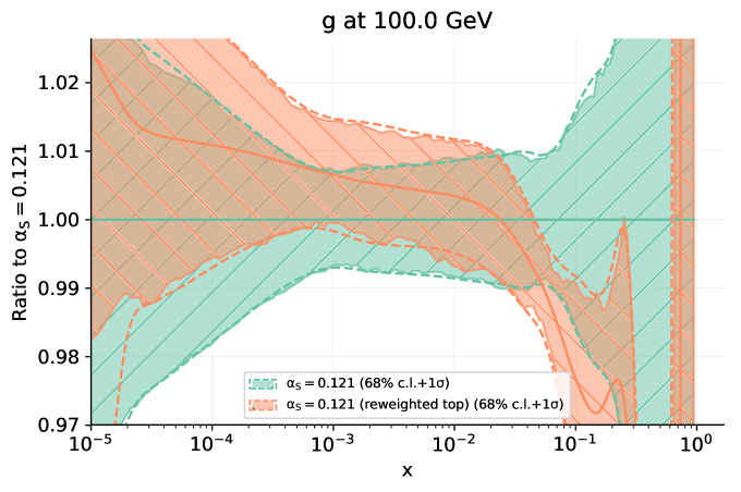
Figure 1: Comparison of gluon PDF between an NNLO-like global fit at NNLO where we have set $\alpha_{S}(M_{Z})=0.121$ and a fit with the only difference that the weight with which the $t\bar{t}$ production data enters the fit has been multiplied by 15. The reweighting causes noticeable decrease in the gluon at large $x$ (but yet roughly within uncertainties) to accommodate the $t\bar{t}$ data which is, which is then described optimally, with $\chi^{2}_{t\bar{t}}/d.o.f.=1.02$, to be compared to $\chi^{2}_{t\bar{t}}/d.o.f.=1.42$ before the reweighing. The improvement of the description of the $t\bar{t}$ data comes at the cost of a deterioration in the global $\chi^{2}$ ($\chi^{2}/d.o.f=1.215$ before the reweighing and $\chi^{2}/d.o.f=1.229$ afterwards).

In summary, we propose that the most statistically rigorous way to produce an $\alpha_{S}$ determination from the measurement $\mathcal{P}$ is to include it in a PDF fit and determine simultaneously $\alpha_{S}$ and the PDFs based on the global $\chi^{2}$ that now includes $\mathcal{P}$ as well as the rest of the data $\mathcal{D}$. Therefore if $\mathcal{P}$ was already included in the $\mathcal{D}$ the result from optimizing the global $\chi^{2}$ profile Eq 2 would be unchanged. Since there is no way to disentangle the $\mathcal{D}$ dependence from Eq. 1, this method is no more PDF dependent than the partial $\chi^{2}$ minimization, but it solves the shortcomings that we have described. The correction on the value of $\alpha_{S}$ when $\mathcal{P}$ is included will either be a small or point to a flaw in the theory, experiment description or fitting methodology. An important advantage is that the process will then be treated using the full fledged PDF fitting machinery (as opposed to a naive minimization of Eq. 2). In particular, this takes care of implementing the correct treatment of the normalization uncertainties, which has been observed to make a significant difference in an $\alpha_{S}$ determination [34]. We conclude that it is questionable to consider hadronic results as independent constrains on $\alpha_{S}$ in World averages, rather than as corrections to the results from the prior PDFs.

3 Preferred values

While we have concluded that the quantities suitable for inclusion in global averages are those based on minimizing the global $\chi^{2}$ profile, Eq. 2, it is nevertheless interesting to define a preferred $\alpha_{S}$ value from a given dataset $\mathcal{P}$. Some possible usages include the assessment of the constraints provided by the measurement, and possibly the study of the higher order corrections (e.g. one could take the dispersion over ensemble of preferred values of a suitable set of processes as an estimate of Missing Higher Order Uncertainty). We first list some desirable properties that such definition should have.

• Independent on the relation between the number of points in the dataset of interest, $N_{\mathcal{P}}$ and those in the global dataset, $N_{\mathcal{D}}$. Clearly, if we are interested in intrinsic physical properties, the number of points in the dataset should not change the result.

• Explicitly depend on the global dataset used in the PDF fit $\mathcal{D}$. Since, as discussed in the previous section, in general we cannot get rid of the dependence on $\mathcal{D}$, it needs to be clearly acknowledged.

• Converge to the determination from $\mathcal{P}$ alone, in the sense described in Sec. 2.2 when it determines $\alpha_{S}$ by itself. While this definition is likely more interesting for smaller, experimentally cleaner, datasets, this is a logical asymptotic property.

The partial $\chi^{2}$ method discussed in Sec. 2.1 has none of these properties and therefore it is not a particularly good definition of preferred value (it may however approximate the third property reasonably well in practice). On the other hand, the exercise illustrated in Fig 1 points at a definition that satisfies them:

Preferred value of $\alpha_{S}$ for the data $\mathcal{P}$

The value of $\alpha_{S}$ that corresponds to the minimum of the global $\chi^{2}$ over values of $\alpha_{S}$ and PDF parameters $\{\theta\}$, when the PDF parameters are restricted to result in a good fit for $\mathcal{P}$ within its experimental uncertainties, for all values of $\alpha_{S}$.

The value is preferred in the sense that the constraints from $\mathcal{P}$ take precedence over those from $\mathcal{D}$, in particular regardless of the number of points, thereby satisfying the first requirement. Once the constrains from $\mathcal{P}$ are enforced, a global $\chi^{2}$ which includes $\mathcal{D}$ is minimized, thus satisfying the second condition.

The main difficulty is to algorithmically specify what a good fit means: Intuitively if the dataset if self consistent at a given value of $\alpha_{S}$, then we require that $\chi_{\mathcal{P}}^{2}/d.o.f\approx 1$. If this is the case at every relevant value of $\alpha_{S}$ then the partial $\chi^{2}_{\mathcal{P}}$ of this reweighed fit is flat and $\alpha_{S}$ is determined based on the agreement with $\mathcal{D}$ (but based on PDFs that have been modified to accommodate $\mathcal{P}$ at all values of $\alpha_{S}$). If $\mathcal{P}$ determines $\alpha_{S}$ by itself (in the sense of Sec 2.2) then the partial $\chi^{2}$ will not be flat and will be used to obtain $\alpha_{S}$. A suitable interpolating procedure between these two situations could be obtained in the NNPDF framework by minimizing as a function of $\{\theta\}$ and $\alpha_{S}$

$$\mathrm{ERF}=\chi^{2}\left[\{\theta\},\alpha_{S},\mathcal{D}\right]+w\chi^{2}\left[\{\theta\},\alpha_{S},\mathcal{P}\right]\ ,$$ (4)

where $w$ is a large number. Because of the cross validation based regularization, the effect of $w$ will saturate either when we reach $\chi_{\mathcal{P}}^{2}/d.o.f\approx 1$, so that only the first therm varies as a function of $\alpha_{S}$, or else, if $\mathcal{P}$ determines $\alpha_{S}$, the curvature of profile will exclusively depend on the second term.

4 Conclusions

We argue that the uncertainties from determinations of $\alpha_{S}(M_{Z})$ from hadronic data can be significatively reduced by interpreting them as corrections on PDF based determinations, equivalent to adding the data to the PDF fit. We propose a definition a preferred value of a parameter that may be advantageous when studying theory uncertainties.

Acknwoledgments

The work of Z.K. is supported by the European Research Council Consolidator Grant “NNLOforLHC2”.

References

- [1] ATLAS Collaboration, G. Aad et al., Observation of a new particle in the search for the Standard Model Higgs boson with the ATLAS detector at the LHC, Phys. Lett. B716 (2012) 1–29, [arXiv:1207.7214].
- [2] CMS Collaboration, S. Chatrchyan et al., Observation of a new boson at a mass of 125 GeV with the CMS experiment at the LHC, Phys. Lett. B716 (2012) 30–61, [arXiv:1207.7235].
- [3] R. K. Ellis, W. J. Stirling, and B. R. Webber, QCD and collider physics. Cambridge University Press, 1996.
- [4] S. Forte, Parton distributions at the dawn of the LHC, Acta Phys.Polon. B41 (2010) 2859, [arXiv:1011.5247].
- [5] NNPDF Collaboration, R. D. Ball et al., Parton distributions from high-precision collider data, Eur. Phys. J. C77 (2017), no. 10 663, [arXiv:1706.00428].
- [6] The NNPDF Collaboration, R. D. Ball et al., Fitting Parton Distribution Data with Multiplicative Normalization Uncertainties, JHEP 05 (2010) 075, [arXiv:0912.2276].
- [7] G. D’Agostini, On the use of the covariance matrix to fit correlated data, Nucl.Instrum.Meth. A346 (1994) 306–311.
- [8] NNPDF Collaboration, R. D. Ball et al., Parton distributions for the LHC Run II, JHEP 04 (2015) 040, [arXiv:1410.8849].
- [9] S. Dulat, T.-J. Hou, J. Gao, M. Guzzi, J. Huston, P. Nadolsky, J. Pumplin, C. Schmidt, D. Stump, and C. P. Yuan, New parton distribution functions from a global analysis of quantum chromodynamics, Phys. Rev. D93 (2016), no. 3 033006, [arXiv:1506.07443].
- [10] L. A. Harland-Lang, A. D. Martin, P. Motylinski, and R. S. Thorne, Parton distributions in the LHC era: MMHT 2014 PDFs, Eur. Phys. J. C75 (2015) 204, [arXiv:1412.3989].
- [11] The NNPDF Collaboration, R. D. Ball et al., Precision determination of electroweak parameters and the strange content of the proton from neutrino deep-inelastic scattering, Nucl. Phys. B823 (2009) 195–233, [arXiv:0906.1958].
- [12] A. Buckley, J. Ferrando, S. Lloyd, K. Nordström, B. Page, et al., LHAPDF6: parton density access in the LHC precision era, Eur.Phys.J. C75 (2015) 132, [arXiv:1412.7420].
- [13] J. Butterworth et al., PDF4LHC recommendations for LHC Run II, J. Phys. G43 (2016) 023001, [arXiv:1510.03865].
- [14] LHC Higgs Cross Section Working Group Collaboration, D. de Florian et al., Handbook of LHC Higgs Cross Sections: 4. Deciphering the Nature of the Higgs Sector, arXiv:1610.07922.
- [15] Particle Data Group Collaboration, C. Patrignani et al., Review of Particle Physics, Chin. Phys. C40 (2016), no. 10 100001.
- [16] S. Alekhin, J. Blümlein, and S. Moch, Parton distribution functions and benchmark cross sections at next-to-next-to-leading order, Physical Review D 86 (2012), no. 5 054009.
- [17] P. Jimenez-Delgado and E. Reya, Dynamical next-to-next-to-leading order parton distributions, Physical Review D 79 (2009), no. 7 074023.
- [18] L. Harland-Lang, A. Martin, P. Motylinski, and R. Thorne, Uncertainties onalpha _s in the mmht2014 global pdf analysis and implications for sm predictions, The European Physical Journal C 75 (2015), no. 9 435.
- [19] R. D. Ball, V. Bertone, L. Del Debbio, S. Forte, A. Guffanti, J. I. Latorre, S. Lionetti, J. Rojo, M. Ubiali, N. Collaboration, et al., Precision nnlo determination of s (mz) using an unbiased global parton set, Physics Letters B 707 (2012), no. 1 66–71.
- [20] CMS Collaboration, S. Chatrchyan et al., Determination of the top-quark pole mass and strong coupling constant from the t t-bar production cross section in pp collisions at = 7 TeV, Phys. Lett. B728 (2014) 496–517, [arXiv:1307.1907]. [Erratum: Phys. Lett.B738,526(2014)].
- [21] V. Andreev et al., Determination of the strong coupling constant in next-to-next-to-leading order QCD using H1 jet cross section measurements, Eur. Phys. J. C77 (2017), no. 11 791, [arXiv:1709.07251].
- [22] B. Bouzid, F. Iddir, and L. Semlala, Determination of the strong coupling constant from ATLAS measurements of the inclusive isolated prompt photon cross section at 7 TeV, arXiv:1703.03959.
- [23] ATLAS Collaboration, M. Aaboud et al., Determination of the strong coupling constant from transverse energy-energy correlations in multijet events at TeV using the ATLAS detector, arXiv:1707.02562.
- [24] T. Klijnsma, S. Bethke, G. Dissertori, and G. P. Salam, Determination of the strong coupling constant from measurements of the total cross section for top-antitop quark production, Eur. Phys. J. C77 (2017), no. 11 778, [arXiv:1708.07495].
- [25] M. Johnson and D. Maître, Strong coupling constant extraction from high-multiplicity Z+jets observables, arXiv:1711.01408.
- [26] ATLAS Collaboration, G. Aad et al., Measurement of the production cross-section using events with b-tagged jets in pp collisions at = 7 and 8 with the ATLAS detector, Eur. Phys. J. C74 (2014), no. 10 3109, [arXiv:1406.5375]. [Addendum: Eur. Phys. J.C76,no.11,642(2016)].
- [27] ATLAS Collaboration, M. Aaboud et al., Measurement of the production cross-section using events with b-tagged jets in pp collisions at =13 TeV with the ATLAS detector, Phys. Lett. B761 (2016) 136–157, [arXiv:1606.02699].
- [28] ATLAS Collaboration, G. Aad et al., Measurements of top-quark pair differential cross-sections in the lepton+jets channel in collisions at TeV using the ATLAS detector, Eur. Phys. J. C76 (2016), no. 10 538, [arXiv:1511.04716].
- [29] CMS Collaboration, V. Khachatryan et al., Measurement of the t-tbar production cross section in the e-mu channel in proton-proton collisions at sqrt(s) = 7 and 8 TeV, JHEP 08 (2016) 029, [arXiv:1603.02303].
- [30] CMS Collaboration, C. Collaboration, Measurement of the top quark pair production cross section using e events in proton-proton collisions at with the CMS detector, .
- [31] CMS Collaboration, V. Khachatryan et al., Measurement of the differential cross section for top quark pair production in pp collisions at 8 TeV, Eur. Phys. J. C75 (2015), no. 11 542, [arXiv:1505.04480].
- [32] M. Czakon, D. Heymes, and A. Mitov, High-precision differential predictions for top-quark pairs at the LHC, Phys. Rev. Lett. 116 (2016), no. 8 082003, [arXiv:1511.00549].
- [33] M. Czakon, D. Heymes, and A. Mitov, Dynamical scales for multi-TeV top-pair production at the LHC, JHEP 04 (2017) 071, [arXiv:1606.03350].
- [34] R. D. Ball, S. Carrazza, L. Del Debbio, S. Forte, Z. Kassabov, J. Rojo, E. Slade, and M. Ubiali, Precision determination of the strong coupling constant within a global PDF analysis, arXiv:1802.03398.